Factorization method versus migration imaging in a waveguide

Abstract

We present a comparative study of two qualitative imaging methods in an acoustic waveguide with sound hard walls. The waveguide terminates at one end and contains unknown obstacles of compact support, to be determined from data gathered by an array of sensors that probe the obstacles with waves and measure the scattered response. The first imaging method, known as the factorization method, is based on the factorization of the far field operator. It is designed to image at single frequency and estimates the support of the obstacles by a Picard range criterion. The second imaging method, known as migration, works either with one or multiple frequencies. It forms an image by backpropagating the measured scattered wave to the search points, using the Green’s function in the empty waveguide. We study the connection between these methods with analysis and numerical simulations.

1 Introduction

Qualitative approaches to inverse scattering problems have been the focus of much activity in the mathematics community [19, 1]. Examples are the linear sampling method [24, 3, 23], the factorization method [30, 32], the orthogonality sampling method [27, 42], the range test method [43], and so on. Some of these methods are connected to MUSIC (MUltiple-SIgnal-Classification) [20, 31], which is another qualitative method that originates from signal processing [47] and is used mostly for imaging point scatterers [28, 10, 40, 2].

Reverse time migration methods and the closely related matched field or matched filtering array data processing techniques are popular in geophysics [22, 7], ocean acoustics [18, 5], radar imaging [25, 21] and elsewhere. These methods form an image by projecting data collected by a sensor array to the replica wave field calculated for a point scatterer at the imaging point. This projection is often called backpropagation. The high frequency versions of these methods are based on the geometrical optics approximation of the replica wave. They are known as Kirchhoff migration [7, 8] in broadband and phase conjugation at a single frequency.

Only some of the qualitative imaging methods, like orthogonality sampling [27, 42], are obviously related to migration. The connection to the factorization method has been made recently in [34], for imaging in free space, using all around measurements. Our goal in this paper is to extend these results to imaging in a waveguide.

Sensor array imaging in waveguides has applications in underwater acoustics [5], imaging of and in tunnels [46, 29, 6], nondestructive evaluation of slender structures [44], and so on. Migration type imaging methods in waveguides with perfectly known geometry have been developed and analyzed in [26, 16, 37, 38, 13, 48, 49] and examples of imaging with experimental validation are in [39, 41]. The case of unknown waveguide geometry is more difficult and is addressed in [12, 11] for randomly perturbed waveguide boundary. We also refer to [9] for a linear sampling approach to imaging in a waveguide with unknown, compactly supported wall deformations. Linear sampling imaging in waveguides with known geometry is studied in [50, 16, 15, 17, 37].

We are interested in the factorization method and its connection to migration, for imaging obstacles in a waveguide with known geometry, that terminates at one end. The termination is motivated by the application of imaging in tunnels and is beneficial because the reflection at the end wall allows a back view of the obstacles. The main difference between the factorization method in a waveguide and in free space is due to the fact that in the waveguide the wave field is a superposition of finitely many propagating modes and infinitely many evanescent modes which cannot be measured in the far field. Thus, imaging must be done only with the propagating modes.

So far, the factorization method in waveguides and cavities has been restricted to using unphysical incident waves as explained in [32, Section 1.7] and [4, 14, 36]. This issue is addressed in [17], by considering incident fields that are pure guided modes and measuring the reflected and transmitted modes before and after the obstacle. Such incident fields could be obtained with a full aperture array of sources, but the measurement of the reflected and transmitted modes may be difficult to realize in some applications.

In this paper we show that the factorization method can be used in a terminated waveguide, for physical incident waves generated by sensors in an array that lies far from the obstacle, on the opposite side of the end wall. We establish a connection between the factorization method and migration imaging and show that obstacles can be localized using only the propagating part of the wave field.

The paper is organized as follows: We begin in section 2 with the formulation of the inverse scattering problem. Then, we discuss in section 3 the factorization method. The connection to migration imaging is in section 4. We assess the results with numerical simulations in section 5 and end with a summary in section 6.

2 The inverse problem

Fig. 1: Imaging setup: An obstacle supported in $\Omega$ in the waveguide ${W}=(-\infty,0)\times\mathcal{X}$ is imaged using measurements collected by an array of sensors lying in the set ${A}$, at range offset $|x_{{A}}|$ from the end wall. The system of coordinates $\vec{{{\itbf x}}}=(x,{{\itbf x}}^{\perp})$ is centered at the end wall, with range coordinate $x<0$ in the waveguide ${W}$ and cross-range coordinate ${{\itbf x}}^{\perp}$ in the cross-section $\mathcal{X}$.

Consider a waveguide that terminates at one end

$${W}=(-\infty,0)\times\mathcal{X}\subset\mathbb{R}^{d},\qquad 2\leq d\leq 3,$$ (2.1)

with cross-section $\mathcal{X}\subset\mathbb{R}^{d-1}$. In two dimensions $(d=2)$ $\mathcal{X}$ is the interval $(0,|\mathcal{X}|)$ of length $|\mathcal{X}|$, whereas in three dimensions $\mathcal{X}$ is a convex and bounded domain with piecewise smooth boundary $\partial\mathcal{X}$. We use the system of coordinates $\vec{{{\itbf x}}}=(x,{{\itbf x}}^{\perp})$ with range $x$ along the axis of the waveguide, starting from the end wall, and with cross-range ${{\itbf x}}^{\perp}\in\mathcal{X}$. To fix ideas, we assume that the waveguide has sound hard walls

$$\partial{W}=\{0\}\times\mathcal{X}\cup(-\infty,0)\times\partial\mathcal{X},$$ (2.2)

and contains sound soft obstacles supported in the compact set $\Omega\subset{W}$, with piecewise smooth boundary $\partial\Omega$. The results are expected to extend to other boundary conditions at $\partial{W}$ and $\partial\Omega$, and also to penetrable scatterers.

The inverse scattering problem is to determine the obstacles from measurements gathered by an array of $n_{{A}}$ sensors located in the set

$${A}=\{x_{{A}}\}\times\mathcal{X},\qquad x_{{A}}<0,$$ (2.3)

that lies on the left side of the obstacles, as illustrated in Figure 1. For simplicity of the presentation we carry out the analysis in the full aperture case, where the array spans the entire set ${A}$.

The array probes the waveguide with a time harmonic wave emitted from one of the sensors, at location $\vec{{{\itbf x}}}_{s}\in{A}$, and measures the echoes $u^{\rm sc}(\vec{{{\itbf x}}}_{r},\vec{{{\itbf x}}}_{s})$ at all the sensor locations $\vec{{{\itbf x}}}_{r}\in{A}$. These echoes are defined in section 2.2. The array data is the response matrix

$$\itbf{U}^{\rm sc}=\big{(}u^{\rm sc}(\vec{{{\itbf x}}}_{r},\vec{{{\itbf x}}}_{s})\big{)}_{1\leq r,s\leq n_{{A}}},$$ (2.4)

gathered by successive illuminations, with one source at a time. We assume in the analysis that the sensor spacing is sufficiently small, so we can make the continuum aperture approximation. This means that we replace sums over the source and receiver indexes $s,r=1,\ldots,n_{{A}}$ by integrals over the aperture ${A}$.

2.1 The incident wave

The probing (incident) wave emitted by the source at $\vec{{{\itbf x}}}_{s}\in{A}$ is defined by the solution of the Helmholtz equation in the empty waveguide. It is the Green’s function $G(\vec{{{\itbf x}}},\vec{{{\itbf x}}}_{s})$ satisfying

$$\big{(}\Delta_{\vec{{{\itbf x}}}}+k^{2}\big{)}G(\vec{{{\itbf x}}},\vec{{{\itbf x}}}_{s}) =-\delta(\vec{{{\itbf x}}}-\vec{{{\itbf x}}}_{s}),\qquad\vec{{{\itbf x}}}\in{W},$$

$$\partial_{\vec{\bm{\nu}}_{{}_{\vec{{{\itbf x}}}}}}G(\vec{{{\itbf x}}},\vec{{{\itbf x}}}_{s}) =0,\hskip 65.04256pt\vec{{{\itbf x}}}\in\partial{W},$$ (2.5)

and the outgoing radiation condition at range $x<x_{{A}}$, stated in Definition 1. Here $\Delta_{\vec{{{\itbf x}}}}$ is the Laplace operator, $k$ is the wavenumber and $\vec{\bm{\nu}}_{{}_{\vec{{{\itbf x}}}}}$ denotes the normal at $\partial{W}$ at point $\vec{{{\itbf x}}}\in\partial{W}$.

Definition 1.

We say that a time harmonic wave field $v(\vec{{{\itbf x}}})\exp(-i\omega t)$, where $\omega$ is the frequency and $t$ is time, satisfies the “outgoing radiation condition” at range $x$ if it consists of backward (left) going modes and decaying evanescent modes. The wave satisfies the “incoming radiation condition” at range $x$ if it consists of forward (right) going modes and decaying evanescent modes.

The mode decomposition of the Green’s function is obtained via separation of variables i.e., by expansion in the $L^{2}(\mathcal{X})$ basis $\{\psi_{j}({{\itbf x}}^{\perp})\}_{j\geq 0}$ of eigenfunctions of the Laplace operator $\Delta_{{{\itbf x}}^{\perp}}$ in the cross-range ${{\itbf x}}^{\perp}$, with Neumann boundary conditions at $\partial\mathcal{X}$. These eigenfunctions can be chosen to be real-valued. They satisfy

$$\Delta_{{{\itbf x}}^{\perp}}\psi_{j}({{\itbf x}}^{\perp}) =-\lambda_{j}\psi_{j}({{\itbf x}}^{\perp}),\qquad{{\itbf x}}^{\perp}\in\mathcal{X},$$

$$\partial_{\bm{\nu}_{{{\itbf x}}^{\perp}}}\psi_{j}({{\itbf x}}^{\perp}) =0,\hskip 65.04256pt{{\itbf x}}^{\perp}\in\partial\mathcal{X},$$ (2.6)

and are orthonormal

$$\int_{\mathcal{X}}d{{\itbf x}}^{\perp}\,\psi_{j}({{\itbf x}}^{\perp})\psi_{j^{\prime}}({{\itbf x}}^{\perp})=\delta_{j,j^{\prime}}.$$ (2.7)

The eigenvalues $-\lambda_{j}$ are real and are ordered as $0=\lambda_{o}<\lambda_{1}\leq\lambda_{2}\leq\ldots.$ They determine the number $J+1$ of propagating modes, where

$$J=\max\{j\in\mathbb{N}:~{}\lambda_{j}\leq k^{2}\}.$$ (2.8)

The modes indexed by $j=0,\ldots,J$ are one dimensional time harmonic waves of the form $\exp[i(\pm\beta_{j}x-\omega t)]$ propagating forward (to the right) and backward (to the left) along the range direction $x$, with wavenumber

$$\beta_{j}=\sqrt{k^{2}-\lambda_{j}},\qquad j=0,\ldots,J.$$ (2.9)

The infinitely many modes indexed by $j>J$ are evanescent waves that decay exponentially away from the source, on the range scale $1/|\beta_{j}|$, where

$$\beta_{j}=i\sqrt{\lambda_{j}-k^{2}},\qquad j>J.$$ (2.10)

We assume throughout that the probing frequency is such that $\beta_{j}\neq 0$ for all $j\geq 0$. Then, the incident field due to the source at $\vec{{{\itbf x}}}_{s}=(x_{{A}},{{\itbf x}}^{\perp}_{s})\in{A}$ is given by

$$u^{\rm inc}(\vec{{{\itbf x}}},\vec{{{\itbf x}}}_{s})=G(\vec{{{\itbf x}}},\vec{{{\itbf x}}}_{s}) =\sum_{j=0}^{J}\frac{i}{\beta_{j}}\psi_{j}({{\itbf x}}^{\perp})\psi_{j}({{\itbf x}}^{\perp}_{s})e^{-i\beta_{j}x_{{A}}}\cos(\beta_{j}x)$$

$$+{\sum_{j>J}}\frac{1}{|\beta_{j}|}\psi_{j}({{\itbf x}}^{\perp})\psi_{j}({{\itbf x}}^{\perp}_{s})e^{|\beta_{j}|x_{{A}}}\cosh(|\beta_{j}|x),$$ (2.11)

at $\vec{{{\itbf x}}}=(x,{{\itbf x}}^{\perp})$ on the right of the array, with range $x\in(x_{{A}},0)$. At points on the left of the array, with range $x<x_{{A}}$, the expression of $G(\vec{{{\itbf x}}},\vec{{{\itbf x}}}_{s})$ is obtained by interchanging $x$ with $x_{{A}}$ in the right hand side of (2.11).

Note that $u^{\rm inc}(\vec{{{\itbf x}}},\vec{{{\itbf x}}}_{s})\exp(-i\omega t)$ satisfies the outgoing radiation condition at range $x<x_{{A}}$, whereas between the array and the end wall there are both forward and backward propagating modes. Because we assume a fixed frequency $\omega$ in the analysis, we drop henceforth the factor $\exp(-i\omega t)$.

2.2 The scattered wave

To define the scattered wave, we make the following standard assumption:

Assumption 1.

The wavenumber $k$ is such that the problem

$$(\Delta_{\vec{{{\itbf x}}}}+k^{2})w(\vec{{{\itbf x}}}) =0,\qquad\vec{{{\itbf x}}}\in{W}\setminus\overline{\Omega},$$

$$\partial_{\vec{\bm{\nu}}_{{}_{\vec{{{\itbf x}}}}}}w(\vec{{{\itbf x}}}) =0,\hskip 20.95781pt\vec{{{\itbf x}}}\in\partial{W},$$

$$w(\vec{{{\itbf x}}}) =0,\hskip 20.95781pt\vec{{{\itbf x}}}\in\partial\Omega,$$

has only the trivial solution $w(\vec{{{\itbf x}}})\equiv 0$ that satisfies either the outgoing or the incoming radiation condition on the left side of $\Omega$, at range

$$x<x_{\Omega}=\inf\{x:\vec{{{\itbf x}}}=(x,{{\itbf x}}^{\perp})\in\Omega\}.$$

Here $\overline{\Omega}$ denotes the closure of $\Omega$.

With this assumption, it is known (see for example [9, Theorem A.4]) that the scattered wave field $u^{\rm sc}(\vec{{{\itbf x}}},\vec{{{\itbf x}}}_{s})$, satisfying

$$(\Delta_{\vec{{{\itbf x}}}}+k^{2})u^{\rm sc}(\vec{{{\itbf x}}},\vec{{{\itbf x}}}_{s}) =0,\qquad\qquad~{}~{}~{}\vec{{{\itbf x}}}\in{W}\setminus\overline{\Omega},$$ (2.12)

$$\partial_{\vec{\bm{\nu}}_{{}_{\vec{{{\itbf x}}}}}}u^{\rm sc}(\vec{{{\itbf x}}},\vec{{{\itbf x}}}_{s}) =0,\hskip 49.86647pt\vec{{{\itbf x}}}\in\partial{W},$$ (2.13)

$$u^{\rm sc}(\vec{{{\itbf x}}},\vec{{{\itbf x}}}_{s}) =-G(\vec{{{\itbf x}}},\vec{{{\itbf x}}}_{s}),~{}~{}~{}\vec{{{\itbf x}}}\in\partial\Omega,$$ (2.14)

and the outgoing radiation condition at range $x<x_{\Omega}$, is well defined. Moreover, $u^{\rm sc}(\cdot,\vec{{{\itbf x}}}_{s})\in H_{\rm loc}^{1}({W}\setminus\overline{\Omega})$.

We will need a second assumption, which holds for all positive $k$ with the exception of a countable set:

Assumption 2.

The wavenumber $k$ is such $k^{2}$ is not an eigenvalue of the negative Laplacian in $\Omega$ with Dirichlet boundary conditions at $\partial\Omega$. That is to say, the problem

$$(\Delta_{\vec{{{\itbf x}}}}+k^{2})w(\vec{{{\itbf x}}}) =0,\qquad\vec{{{\itbf x}}}\in\Omega,$$

$$w(\vec{{{\itbf x}}}) =0,\hskip 20.95781pt\vec{{{\itbf x}}}\in\partial\Omega,$$

has only the trivial solution $w(\vec{{{\itbf x}}})\equiv 0$ in $\Omega$.

3 Imaging with the factorization method

We now describe the factorization method for solving the inverse scattering problem. We begin in section 3.1 with the definition of the relevant operators and then describe the method in section 3.2.

3.1 The operators

Consider the linear integral operator $\mathcal{N}:L^{2}({A})\to L^{2}({A})$,

$$\mathcal{N}g(\vec{{{\itbf x}}})=\int_{{A}}dS_{\vec{{{\itbf y}}}}\,u^{\rm sc}(\vec{{{\itbf x}}},\vec{{{\itbf y}}})g(\vec{{{\itbf y}}}),\qquad\vec{{{\itbf x}}}\in{A},~{}~{}\forall\,g\in L^{2}({A}),$$ (3.15)

with kernel given by the measured scattered field $u^{\rm sc}$ at the array. This is called in the literature, depending on the authors, either the far field or the near field operator. It defines the scattered wave $\mathcal{N}g$ received at the array, due to an illumination $g$ from all the sources in ${A}$. Because $u^{\rm sc}(\cdot,\vec{{{\itbf x}}}_{s})\in H_{\rm loc}^{1}({W}\setminus\overline{\Omega})$, the range of $\mathcal{N}$ lies in $H^{\frac{1}{2}}({A})$, but we view $\mathcal{N}$ as an operator from $L^{2}({A})$ to $L^{2}({A})$. As shown in the next section, $\mathcal{N}$ can be factorized in terms of three linear operators $\mathcal{T}$, $\Lambda$ and $\mathcal{S}$ that we now define:

The operator $\mathcal{T}:L^{2}({A})\to H^{\frac{1}{2}}(\partial\Omega)$ maps functions defined at the array to functions defined at the boundary $\partial\Omega$ of the obstacles,

$$\mathcal{T}g(\vec{{{\itbf z}}})=\int_{{A}}dS_{\vec{{{\itbf y}}}}\,G(\vec{{{\itbf z}}},\vec{{{\itbf y}}})g(\vec{{{\itbf y}}}),\qquad\vec{{{\itbf z}}}\in\partial\Omega,~{}~{}\forall\,g\in L^{2}({A}).$$ (3.16)

Its adjoint $\mathcal{T}^{\star}:H^{-\frac{1}{2}}(\partial\Omega)\to L^{2}({A})$ is given by

$$\mathcal{T}^{\star}h(\vec{{{\itbf x}}})=\int_{\partial\Omega}dS_{\vec{{{\itbf z}}}}\,\overline{G(\vec{{{\itbf z}}},\vec{{{\itbf x}}})}h(\vec{{{\itbf z}}}),\qquad\vec{{{\itbf x}}}\in{A},~{}~{}\forall\,h\in H^{-\frac{1}{2}}(\partial\Omega),$$ (3.17)

where the bar denotes throughout the complex conjugate. This adjoint is defined using the inner product

$$\big{(}f,g\big{)}_{{A}}=\int_{{A}}dS_{\vec{{{\itbf x}}}}\,\overline{f(\vec{{{\itbf x}}})}g(\vec{{{\itbf x}}}),\qquad\forall\,f,g\in L^{2}({A}),$$ (3.18)

and the duality pairing

$$\left<f,g\right>_{\partial\Omega}=\int_{\partial\Omega}dS_{\vec{{{\itbf x}}}}\,\overline{f(\vec{{{\itbf x}}})}g(\vec{{{\itbf x}}}),\qquad\forall\,f\in H^{\frac{1}{2}}(\partial\Omega),~{}~{}\forall\,g\in H^{-\frac{1}{2}}(\partial\Omega),$$ (3.19)

meaning that

$$\big{(}f,\mathcal{T}^{\star}g\big{)}_{{A}}=\left<\mathcal{T}f,g\right>_{\partial\Omega},\qquad\forall\,f\in L^{2}({A}),~{}~{}\forall\,g\in H^{-\frac{1}{2}}(\partial\Omega).$$ (3.20)

The operator $\Lambda:H^{\frac{1}{2}}(\partial\Omega)\to H^{-\frac{1}{2}}(\partial\Omega)$ is the Dirichlet to Neumann map

$$\Lambda f(\vec{{{\itbf x}}})=h(\vec{{{\itbf x}}}),\qquad\vec{{{\itbf x}}}\in\partial\Omega,~{}~{}\forall\,f\in H^{\frac{1}{2}}(\partial\Omega),$$ (3.21)

where $h\in H^{-\frac{1}{2}}(\partial\Omega)$ is the solution of

$$\int_{\partial\Omega}dS_{\vec{{{\itbf z}}}}\,\overline{G(\vec{{{\itbf x}}},\vec{{{\itbf z}}})}h(\vec{{{\itbf z}}})=-f(\vec{{{\itbf x}}}),\qquad\vec{{{\itbf x}}}\in\partial\Omega.$$ (3.22)

The solvability of (3.22) is established in [16, Section 4.2], under the Assumption 2, and [16, Proposition 1] gives that $\Lambda$ is an isomorphism.

The scattering operator $\mathcal{S}$ maps incoming to outgoing waves at ${A}$. To define it, we introduce the function spaces

$$\mathscr{H}(W\setminus\overline{\Omega}) =\Big{\{}w\in H_{\rm loc}^{1}(W\setminus\overline{\Omega}):~{}~{}(\Delta_{\vec{{{\itbf x}}}}+k^{2})w(\vec{{{\itbf x}}})=0~{}{\rm in}~{}W\setminus\overline{\Omega},$$

$$\hskip 137.31255pt\partial_{\vec{\bm{\nu}}_{{}_{\vec{{{\itbf x}}}}}}w(\vec{{{\itbf x}}})=0~{}{\rm on}~{}\partial W\Big{\}},$$ (3.23)

$$\mathscr{H}^{\rm out}(A) =\Big{\{}w|_{{A}}:~{}w\in\mathscr{H}(W\setminus\overline{\Omega}),~{}~{}w\mbox{ satisfies the outgoing }$$

$$\hskip 101.17755pt\mbox{radiation condition at }x<x_{\Omega}\Big{\}},$$ (3.24)

$$\mathscr{H}^{\rm in}(A) =\Big{\{}w|_{{A}}:~{}w\in\mathscr{H}(W\setminus\overline{\Omega}),~{}~{}w\mbox{ satisfies the incoming}$$

$$\hskip 101.17755pt\mbox{radiation condition at }x<x_{\Omega}\Big{\}},$$ (3.25)

where $w|_{{A}}$ denotes the trace of $w$ on ${A}$. The operator $\mathcal{S}:\mathscr{H}^{\rm in}(A)\to\mathscr{H}^{\rm out}(A)$ is defined by

$$\mathcal{S}v(\vec{{{\itbf x}}})=w(\vec{{{\itbf x}}}),\qquad\vec{{{\itbf x}}}\in{A},~{}~{}\forall\,v\in\mathscr{H}^{\rm in}(A),$$ (3.26)

where $w(\vec{{{\itbf x}}})\in\mathscr{H}(W\setminus\overline{\Omega})$ satisfies the boundary condition

$$w(\vec{{{\itbf x}}})=v(\vec{{{\itbf x}}}),\qquad\vec{{{\itbf x}}}\in\partial\Omega,$$ (3.27)

and the outgoing radiation condition at range $x<x_{\Omega}$. Moreover, $\mathcal{S}$ is invertible, with inverse $\mathcal{S}^{-1}:\mathscr{H}^{\rm out}(A)\to\mathscr{H}^{\rm in}(A)$ defined by

$$\mathcal{S}^{-1}w(\vec{{{\itbf x}}})=v(\vec{{{\itbf x}}}),\qquad\vec{{{\itbf x}}}\in{A},~{}~{}\forall\,w\in\mathscr{H}^{\rm out}(A),$$ (3.28)

where $v(\vec{{{\itbf x}}})\in\mathscr{H}(W\setminus\overline{\Omega})$ satisfies the boundary condition

$${v(\vec{{{\itbf x}}})=w(\vec{{{\itbf x}}})},\qquad\vec{{{\itbf x}}}\in\partial\Omega,$$ (3.29)

and the incoming radiation condition at range $x<x_{\Omega}$.

3.2 The factorization method

The imaging is based on the operator

$$\mathcal{F}:L^{2}({A})\to L^{2}({A}),~{}~{}~{}\mathcal{F}=\mathcal{S}^{-1}\mathcal{N},$$ (3.30)

which is defined in terms of the array measurements, as stated in the following lemma:

Lemma 2.

Any $\phi\in L^{2}({A})$ can be written as

$$\phi(\vec{{{\itbf x}}})=\phi^{(1)}(\vec{{{\itbf x}}})+i\phi^{(2)}(\vec{{{\itbf x}}}),$$ (3.31)

for $\vec{{{\itbf x}}}=(x_{{A}},{{\itbf x}}^{\perp})\in{A}$, with

$$\phi^{(l)}(\vec{{{\itbf x}}})=\sum_{j=0}^{J}\frac{\alpha_{j}^{(l)}}{i}\psi_{j}({{\itbf x}}^{\perp})e^{i\beta_{j}x_{{A}}}+\sum_{j>J}\alpha_{j}^{(l)}\psi_{j}({{\itbf x}}^{\perp}),$$ (3.32)

and $\alpha_{j}^{(l)}\in\mathbb{R}$, for all $j\geq 0$ and $l=1,2$. Furthermore,

$$\mathcal{F}\phi(\vec{{{\itbf x}}})=\mathcal{F}\phi^{(1)}(\vec{{{\itbf x}}})+i\mathcal{F}\phi^{(2)}(\vec{{{\itbf x}}}),$$ (3.33)

where

$$\mathcal{F}\phi^{(l)}(\vec{{{\itbf x}}})=\int_{{A}}dS_{\vec{{{\itbf y}}}}\,\overline{u^{\rm sc}(\vec{{{\itbf x}}},\vec{{{\itbf y}}})\phi^{(l)}(\vec{{{\itbf y}}})},\qquad\vec{{{\itbf x}}}\in{A},~{}~{}l=1,2.$$ (3.34)

The proof of this lemma is in Appendix A and the decomposition (3.31) is obtained from the expansion of $\phi$ in the $L^{2}({A})$ eigenbasis $\{\psi_{j}({{\itbf x}}^{\perp})\}_{j\geq 0},$

$$\phi(\vec{{{\itbf x}}})=\sum_{j=0}^{\infty}\gamma_{j}\psi_{j}({{\itbf x}}^{\perp}),\qquad\vec{{{\itbf x}}}=(x_{{A}},{{\itbf x}}^{\perp})\in{A},$$ (3.35)

with coefficients $\gamma_{j}\in\mathbb{C}$. The real valued $\alpha_{j}^{(1)}$ and $\alpha_{j}^{(2)}$ in (3.32) are defined in terms of these coefficients by

$$\alpha_{j}^{(1)}+i\alpha_{j}^{(2)} =\left\{\begin{array}[]{ll}i\gamma_{j}e^{-i\beta_{j}x_{A}},&\mbox{if}~{}~{}j=0,\ldots,J,\\ \gamma_{j},&\mbox{if}~{}~{}j>J.\end{array}\right.$$ (3.38)

Theorem 3.

The operator $\mathcal{F}$ has the factorization

$$\mathcal{F}=\mathcal{T}^{\star}\Lambda\mathcal{T},$$ (3.39)

and the operators defined in (3.16) and (3.21)) satisfy the following properties:
(i) The operator $\mathcal{T}$ is compact and injective.
(ii) Let $\Lambda^{\star}:H^{\frac{1}{2}}(\partial\Omega)\to H^{-\frac{1}{2}}(\partial\Omega)$ be the adjoint of $\Lambda$, defined by

$$\left<\Lambda f,g\right>_{\partial\Omega}=\left<f,\Lambda^{\star}g\right>_{\partial\Omega},\qquad\forall\,f,g\in H^{\frac{1}{2}}(\partial\Omega),$$ (3.40)

using the duality pairing (3.19). Define the self-adjoint operators $\Im(\Lambda)=\big{(}\Lambda-\Lambda^{\star}\big{)}/(2i)$ and $\Re(\Lambda)=\big{(}\Lambda+\Lambda^{\star}\big{)}/2$. Then, $-\Im(\Lambda)$ is positive semi-definite,

$${-\left<\Im(\Lambda)f,f\right>_{\partial\Omega}}\geq 0,\qquad\forall\,f\in H^{\frac{1}{2}}(\partial\Omega),$$ (3.41)

and ${-\Re(\Lambda)}$ is the sum of a positive definite, self-adjoint operator and a compact operator.

This result, proved in Appendix B, and the next lemma, proved in Appendix C, are the theoretical foundation of the factorization method.

Lemma 4.

Let $\vec{{{\itbf z}}}\in(x_{{A}},0)\times\mathcal{X}$ be a search point. Then, $\vec{{{\itbf z}}}\in\Omega$ if and only if $\overline{G(\cdot,\vec{{{\itbf z}}})}|_{{A}}\in\mbox{range}(\mathcal{T}^{\star}).$

The range test in Lemma 4 cannot be used directly to determine the support $\Omega$ of the obstacles, because $\mathcal{T}^{\star}$ is not known. However, [33, Theorem 2.1] shows that $\Omega$ can be determined using a new operator

$$\mathcal{F}_{\#}=\big{|}\Re(\mathcal{F})\big{|}-\Im(\mathcal{F})$$ (3.42)

where

$$\Re(\mathcal{F})=\frac{\big{(}\mathcal{F}+\mathcal{F}^{\star}\big{)}}{2},\qquad\Im(\mathcal{F})=\frac{\big{(}\mathcal{F}-\mathcal{F}^{\star}\big{)}}{2i},$$ (3.43)

and $\big{|}\Re(\mathcal{F})\big{|}$ is defined in the standard way, using the spectral representation of $\Re(\mathcal{F})$. Similarly, we define

$$\Re(\Lambda)=\frac{(\Lambda+\Lambda^{\star})}{2},\qquad\Im(\Lambda)=\frac{(\Lambda-\Lambda^{\star})}{2i},\qquad\Lambda_{\#}=\big{|}\Re(\Lambda)\big{|}-\Im(\Lambda),$$ (3.44)

and conclude from the proof of [33, Theorem 2.1] that

$$\mathcal{F}_{\#}=\mathcal{T}^{*}\Lambda_{\#}\mathcal{T}.$$ (3.45)

We deduce from Theorem 3 and (3.42) that $\mathcal{F}_{\#}$ is positive definite, so we can take its square root $\mathcal{F}_{\#}^{\frac{1}{2}}$. The following result follows from Theorem 3, Lemma 4 and [33, Theorem 2.1].

Theorem 5.

Let $\vec{{{\itbf z}}}\in(x_{{A}},0)\times\mathcal{X}$ be a search point in the waveguide, between the array and the end wall. Then, $\vec{{{\itbf z}}}\in\Omega$ if and only if

$$\mbox{inf}\Big{\{}\big{(}{\mathcal{F}^{\#}}\varphi,\varphi\big{)}_{{A}}:~{}\varphi\in L^{2}({A}),~{}~{}\big{(}\overline{G(\cdot,\vec{{{\itbf z}}})},\varphi\big{)}_{{A}}=1\Big{\}}>0,$$ (3.46)

or, equivalently, if and only if

$$\overline{G(\cdot,\vec{{{\itbf z}}})}|_{{A}}\in\mbox{range}\big{(}\mathcal{F}_{\#}^{\frac{1}{2}}\big{)}.$$ (3.47)

The factorization method uses the condition (3.47) and a Picard range criterion to define the sampling function

$$g_{\#}(\vec{{{\itbf z}}})=\sum_{j=1}^{\infty}\frac{\big{|}\big{(}\overline{G(\cdot,\vec{{{\itbf z}}})},\varphi_{j}\big{)}_{{A}}\big{|}^{2}}{\mu_{j}},$$ (3.48)

where $\varphi_{j}$ are the eigenfunctions of $\mathcal{F}_{\#}$ for the eigenvalues $\mu_{j}$. This function should be bounded if and only if $\vec{{{\itbf z}}}\in\Omega$.

In practice, we can work only with the propagating part of the scattered field, because the array is at large distance from the obstacle. Thus, instead of $\mathcal{F}$ defined as in Lemma 2, we use its projection on the subspace

$${\mathscr{P}}=\mbox{span}\{\psi_{0},\ldots,\psi_{J}\}\subset L^{2}({A}).$$ (3.49)

The projection is the $(J+1)\times(J+1)$ matrix

$$\mathcal{F}^{{\mathscr{P}}}=\Big{(}\big{(}\mathcal{F}\psi_{j},\psi_{l}\big{)}_{{A}}\Big{)}_{0\leq j,l\leq J},$$ (3.50)

which defines in turn the $(J+1)\times(J+1)$ Hermitian, positive definite matrix

$$\mathcal{F}^{{\mathscr{P}}}_{\#}=\big{|}\Re(\mathcal{F}^{{\mathscr{P}}})\big{|}+{|\Im(\mathcal{F}^{{\mathscr{P}}})|}.$$ (3.51)

The implementation of the factorization method in section 5 is based on the Picard range criterium for the square root of (3.51), so the series in (3.48) becomes a finite sum with $J+1$ terms. The resulting image is expected to be larger outside the obstacle, and the numerical results illustrate that this is indeed the case. However, the equivalent of Theorem 5 is not yet established for the projection $\mathcal{F}^{{\mathscr{P}}}_{\#}$ to the propagating modes.

4 Connection to migration imaging

We describe in section 4.1 the classic migration imaging function, where the scattered wave $u^{\rm sc}$ is backpropagated to the search point $\vec{{{\itbf z}}}$ using the Green’s function in the empty waveguide. Then, we give in section 4.2 a slight modification of the migration imaging function, where the backpropagation is done with the second derivative of the Green’s function, for improved focusing of the image. The connection to the factorization method is in section 4.3.

4.1 Migration imaging

Let $\mathbb{P}:L^{2}({A})\to{\mathscr{P}}$ be the orthogonal projector from $L^{2}({A})$ to ${\mathscr{P}}$ and denote by

$$G_{{\mathscr{P}}}(\cdot,\vec{{{\itbf z}}})\big{|}_{{A}}=\mathbb{P}G(\cdot,\vec{{{\itbf z}}})\big{|}_{{A}}$$ (4.52)

the propagating part of the Green’s function evaluated at the array. The classic migration imaging function is given by

$${\cal J}(\vec{{{\itbf z}}})=\iint_{{A}}dS_{\vec{{{\itbf x}}}}dS_{\vec{{{\itbf y}}}}\,u^{\rm sc}(\vec{{{\itbf x}}},\vec{{{\itbf y}}})\overline{G_{{\mathscr{P}}}(\vec{{{\itbf x}}},\vec{{{\itbf z}}})}\overline{G_{{\mathscr{P}}}(\vec{{{\itbf y}}},\vec{{{\itbf z}}})},$$ (4.53)

Because the array is far from the obstacles, we neglect the evanescent part of the measured $u^{\rm sc}$ and backropagate it to $\vec{{{\itbf z}}}$ using (4.52).

Note from (2.11) that $\overline{G_{{\mathscr{P}}}(\cdot,\vec{{{\itbf z}}})\big{|}_{{A}}}$ is of the form (3.31), so we can use (3.34), the factorization (3.39) and the duality relation (3.20) to rewrite (4.53) as

$${\cal J}(\vec{{{\itbf z}}})=\big{(}\mathcal{F}\overline{G_{{\mathscr{P}}}(\cdot,\vec{{{\itbf z}}})\big{|}_{{A}}},\overline{G_{{\mathscr{P}}}(\cdot,\vec{{{\itbf z}}})\big{|}_{{A}}}\big{)}_{{A}}=\left<\Lambda\mathcal{T}\overline{G_{{\mathscr{P}}}(\cdot,\vec{{{\itbf z}}})\big{|}_{{A}}},\mathcal{T}\overline{G_{{\mathscr{P}}}(\cdot,\vec{{{\itbf z}}})\big{|}_{{A}}}\right>_{\partial\Omega}.$$ (4.54)

We also obtain from definition (3.16) and the orthogonality relation (2.7) that

$$K_{0}(\vec{{{\itbf x}}},\vec{{{\itbf z}}}) =\mathcal{T}\overline{G_{{\mathscr{P}}}(\cdot,\vec{{{\itbf z}}})\big{|}_{{A}}}(\vec{{{\itbf x}}})=\int_{{A}}dS_{\vec{{{\itbf y}}}}\,G(\vec{{{\itbf x}}},\vec{{{\itbf y}}})\overline{G_{{\mathscr{P}}}(\vec{{{\itbf y}}},\vec{{{\itbf z}}})}$$

$$=\sum_{j=0}^{J}\frac{1}{\beta_{j}^{2}}\psi_{j}({{\itbf x}}^{\perp})\psi_{j}({{\itbf z}}^{\perp})\cos(\beta_{j}x)\cos(\beta_{j}z),\qquad\vec{{{\itbf x}}}=(x,{{\itbf x}}^{\perp})\in\partial\Omega.$$ (4.55)

In (4.54) we calculate the duality pairing

$$\mathcal{J}(\vec{{{\itbf z}}})=\left<\Lambda K_{0}(\cdot,\vec{{{\itbf z}}})\big{|}_{{A}},K_{0}(\cdot,\vec{{{\itbf z}}})\big{|}_{{A}}\right>_{\partial\Omega}=\int_{\partial\Omega}dS_{\vec{{{\itbf x}}}}\,\overline{h(\vec{{{\itbf x}}})}K_{0}(\vec{{{\itbf x}}},\vec{{{\itbf z}}}),$$ (4.56)

where $h=\Lambda K_{0}(\cdot,\vec{{{\itbf z}}})\big{|}_{{A}}$ is the solution of

$$\int_{\partial\Omega}dS_{\vec{{{\itbf y}}}}\,\overline{G(\vec{{{\itbf x}}},\vec{{{\itbf y}}})}h(\vec{{{\itbf y}}})=-K_{0}(\vec{{{\itbf x}}},\vec{{{\itbf z}}}),\qquad\vec{{{\itbf x}}}\in\partial\Omega.$$ (4.57)

Because $\Lambda$ is an isomorphism, we have that $\|h\|_{H^{-\frac{1}{2}}(\partial\Omega)}$ is large when $\|K_{0}(\cdot,\vec{{{\itbf z}}})\|_{H^{\frac{1}{2}}(\partial\Omega)}$ is large, so the focusing of the imaging function (4.56) depends on how sharply peaked the kernel $\eqref{eq:Mi3}$ is at $\vec{{{\itbf x}}}=\vec{{{\itbf z}}}$.

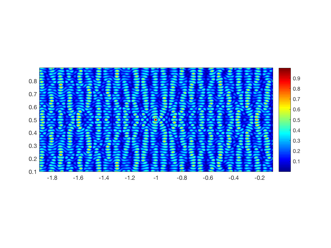
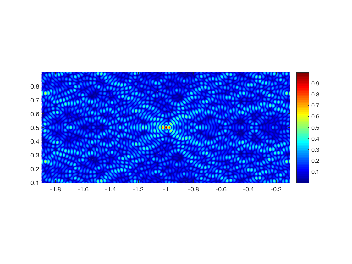
Fig. 2: The absolute value of the kernel $\mathcal{K}_{0}(\vec{{{\itbf x}}},\vec{{{\itbf z}}})$ (left) and $\mathcal{K}(\vec{{{\itbf x}}},\vec{{{\itbf z}}})$ (right) in a two dimensional waveguide with $50$ propagating modes. Both kernels are normalized by their maximum value. The point $\vec{{{\itbf x}}}=(-|\mathcal{X}|,|\mathcal{X}|/2)$ is fixed and the search domain of $\vec{{{\itbf z}}}=(z,{{\itbf z}}^{\perp})$ is indicated in the labels, in units of $|\mathcal{X}|$. The abscissa is $z$ and ordinate is ${{\itbf z}}^{\perp}$, in units of $|\mathcal{X}|$.

We display in the left plot of Figure 2 the kernel $K_{0}(\vec{{{\itbf x}}},\vec{{{\itbf z}}})$ in a two dimensional waveguide with $50$ propagating modes (see also Figure 3). We note that while $K_{0}(\vec{{{\itbf x}}},\vec{{{\itbf z}}})$ has a peak at $\vec{{{\itbf x}}}=\vec{{{\itbf z}}}$, there are many other peaks. In the next section we modify slightly the imaging function, by backpropagating with the second range derivative of $G_{{\mathscr{P}}}$. This results in the better focused kernel $K(\vec{{{\itbf x}}},\vec{{{\itbf z}}})$ displayed in the right plot of Figure 2.

4.2 A modified migration imaging function

Instead of using $\overline{G_{{\mathscr{P}}}(\cdot,\vec{{{\itbf z}}})\big{|}_{{A}}}$ to backpropagate the measured $u^{\rm sc}$ to the imaging point $\vec{{{\itbf z}}}$, consider

$$\varphi_{\vec{{{\itbf z}}}}(\vec{{{\itbf x}}}) =C_{\vec{{{\itbf z}}}}\sum_{j=0}^{J}\frac{\beta_{j}}{i}\psi_{j}({{\itbf z}}^{\perp})\psi_{j}({{\itbf x}}^{\perp})e^{i\beta_{j}x_{{A}}}\cos(\beta_{j}z)$$

$$=-C_{\vec{{{\itbf z}}}}\partial_{x}^{2}\overline{G_{{\mathscr{P}}}(\vec{{{\itbf x}}},\vec{{{\itbf z}}})}\big{|}_{\vec{{{\itbf x}}}\in{A}},\qquad\vec{{{\itbf x}}}=(x_{{A}},{{\itbf x}}^{\perp})\in{A},$$ (4.58)

where $C_{\vec{{{\itbf z}}}}$ is a positive normalization constant so that

$$\big{(}\overline{G(\cdot,\vec{{{\itbf z}}})},\varphi_{\vec{{{\itbf z}}}}\big{)}_{{A}}=C_{\vec{{{\itbf z}}}}\sum_{j=0}^{J}\psi_{j}^{2}({{\itbf z}}^{\perp})\cos^{2}(\beta_{j})=1.$$ (4.59)

This function $\varphi_{\vec{{{\itbf z}}}}$ is of the form (3.32), so we can calculate $\mathbb{P}\mathcal{F}\varphi_{\vec{{{\itbf z}}}}$ from the measurements at the array, using Lemma 2 and the matrix (3.50).

The modified migration type imaging function is

$$\mathcal{J}_{\rm mig}(\vec{{{\itbf z}}})=-\Im\Big{[}\big{(}\mathcal{F}\varphi_{\vec{{{\itbf z}}}},\varphi_{\vec{{{\itbf z}}}}\big{)}_{{A}}\Big{]}=-\Im\Big{[}\big{(}\mathbb{P}\mathcal{F}\varphi_{\vec{{{\itbf z}}}},\varphi_{\vec{{{\itbf z}}}}\big{)}_{{A}}\Big{]}=-\big{(}\Im(\mathcal{F})\varphi_{\vec{{{\itbf z}}}},\varphi_{\vec{{{\itbf z}}}}\big{)}_{{A}},$$ (4.60)

where we used the orthogonality relation (2.7), definition (3.43) and the identity

$$\big{(}\mathcal{F}^{\star}\varphi_{\vec{{{\itbf z}}}},\varphi_{\vec{{{\itbf z}}}}\big{)}_{{A}}=\big{(}\varphi_{\vec{{{\itbf z}}}},\mathcal{F}\varphi_{\vec{{{\itbf z}}}}\big{)}_{{A}}=\overline{\big{(}\mathcal{F}\varphi_{\vec{{{\itbf z}}}},\varphi_{\vec{{{\itbf z}}}}\big{)}_{{A}}}.$$

We take the imaginary part in order to relate (4.60) to the factorization method. Using equation (3.39) in (4.60) we obtain

$$\mathcal{J}_{\rm mig}(\vec{{{\itbf z}}})=-\left<\Im(\Lambda)\mathcal{K}(\cdot,\vec{{{\itbf z}}}),\mathcal{K}(\cdot,\vec{{{\itbf z}}})\right>_{\partial\Omega},$$ (4.61)

where we introduced the kernel

$$K(\vec{{{\itbf x}}},\vec{{{\itbf z}}}) =\mathcal{T}\varphi_{\vec{{{\itbf z}}}}(\vec{{{\itbf x}}})=\int_{{A}}dS_{\vec{{{\itbf y}}}}\,G(\vec{{{\itbf x}}},\vec{{{\itbf y}}})\varphi_{\vec{{{\itbf z}}}}(\vec{{{\itbf y}}})=C_{\vec{{{\itbf z}}}}\sum_{j=0}^{J}\psi_{j}({{\itbf x}}^{\perp})\psi_{j}({{\itbf z}}^{\perp})\cos(\beta_{j}x)\cos({\beta_{j}}z)$$

$$=C_{\vec{{{\itbf z}}}}\Re\Big{[}\partial_{x}G_{{\mathscr{P}}}(\vec{{{\itbf x}}},\vec{{{\itbf z}}})\Big{]},\qquad\vec{{{\itbf x}}}=(x,{{\itbf x}}^{\perp})\in\partial\Omega.$$ (4.62)

This kernel is peaked at $\vec{{{\itbf x}}}=\vec{{{\itbf z}}}$ and decays with $|\vec{{{\itbf x}}}-\vec{{{\itbf z}}}|$ as illustrated in the right plots of Figures 2 and 3.

Because $\Lambda\mathcal{K}(\cdot,\vec{{{\itbf z}}})\big{|}_{\partial\Omega}$ is bounded in $H^{\frac{1}{2}}(\partial\Omega)$, the imaging function (4.61) is bounded above in terms of $\|\mathcal{K}(\cdot,\vec{{{\itbf z}}})\|_{H^{\frac{1}{2}}(\partial\Omega)}$ and therefore of $\|\mathcal{K}(\cdot,\vec{{{\itbf z}}})\|_{H^{1}(\Omega)}$. The latter norm is small when $\vec{{{\itbf z}}}$ is far from $\Omega$, as illustrated in Figure 3. By Theorem 3, the operator $-\Im(\Lambda)$ is self-adjoint and positive semi-definite, so we expect that the imaging function (4.61) is large for search points $\vec{{{\itbf z}}}$ near $\partial\Omega$, as long as $K(\cdot,\vec{{{\itbf z}}})$ is not in the null space of $\Im(\Lambda)$.

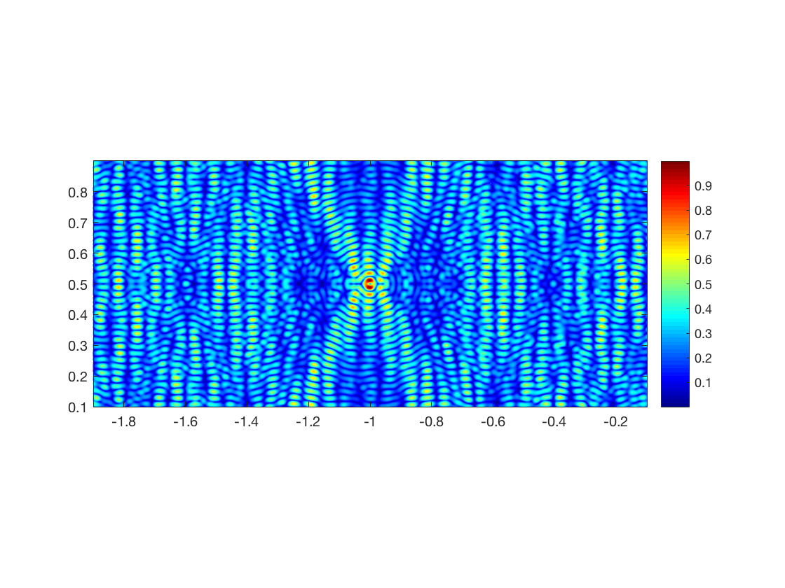
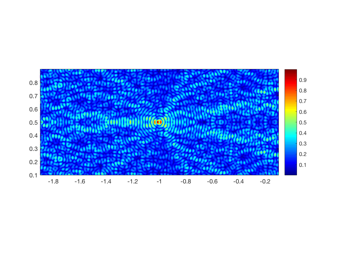
Fig. 3: We display $\|\mathcal{K}_{0}(\cdot,\vec{{{\itbf z}}})\|_{H^{1}(\Omega)}$ (left) and $\|\mathcal{K}(\cdot,\vec{{{\itbf z}}})\|_{H^{1}(\Omega)}$ (right) in a two dimensional waveguide with $50$ propagating modes, where $\Omega$ is a square centered at $(-|\mathcal{X}|,|\mathcal{X}|/2)$, of side length $0.02|\mathcal{X}|$. In both plots we normalize to maximum value $1$. The search domain of $\vec{{{\itbf z}}}=(z,{{\itbf z}}^{\perp})$ is indicated in the labels, in units of $|\mathcal{X}|$. The abscissa is $z$ and ordinate is ${{\itbf z}}^{\perp}$, in units of $|\mathcal{X}|$.

The next theorem sheds more light on the behavior of $\mathcal{J}_{\rm mig}(\vec{{{\itbf z}}})$ for search points near $\Omega$. To state it, let $\itbf{U}^{{\rm sc},{\mathscr{P}}}$ be the $(J+1)\times(J+1)$ matrix obtained by projecting the measured scattered field $u^{\rm sc}$ on the finite dimensional subspace (3.49). The entries of this matrix are

$$U^{{\rm sc},{\mathscr{P}}}_{j,l}=\iint_{{A}}dS_{\vec{{{\itbf x}}}}dS_{\vec{{{\itbf y}}}}\,u^{\rm sc}(\vec{{{\itbf x}}},\vec{{{\itbf y}}})\psi_{j}({{\itbf x}}^{\perp})\psi_{l}({{\itbf y}}^{\perp}),\qquad j,l=0,\ldots,J,$$ (4.63)

and we note that $\itbf{U}^{{\rm sc},{\mathscr{P}}}$ is complex symmetric, by reciprocity, but it is not Hermitian. The singular value decomposition of $\itbf{U}^{{\rm sc},{\mathscr{P}}}$ is of the form

$$\itbf{U}^{{\rm sc},{\mathscr{P}}}=\itbf{V}\bm{\mathfrak{S}}\itbf{V}^{T},$$ (4.64)

where ${\itbf V}$ is unitary, with columns ${{\itbf v}}_{j}$ for $j=1,\ldots,J+1$, and $\bm{\mathfrak{S}}$ is the diagonal matrix of singular values, in decreasing order. Typically, the matrix $\itbf{U}^{{\rm sc},{\mathscr{P}}}$ is rank defficient, with rank $r<J+1$. Its null space is spanned by the right singular vectors $\overline{{{\itbf v}}_{j}}$, for $j=r+1,\ldots,J+1$. We denote by $\overline{V_{j,l}}$ the entries of these singular vectors, and use them to define the following subspace of ${\mathscr{P}}$, of dimension $J-r+1$,

$${\mathscr{P}}_{0}=\mbox{span}\Big{\{}\sum_{j=0}^{J}\overline{V_{j+1,l}}\psi_{j}({{\itbf x}}^{\perp}),~{}~{}l=r+1,\ldots,J+1\Big{\}}.$$ (4.65)

This is in the null space of the operator $\mathbb{P}\mathcal{N}:L^{2}({A})\to{\mathscr{P}}$. The orthogonal complement of ${\mathscr{P}}_{0}$ in ${\mathscr{P}}$ is denoted by ${\mathscr{P}}_{0}^{\perp}$, so we can write

$${\mathscr{P}}={\mathscr{P}}_{0}\oplus{\mathscr{P}}_{0}^{\perp}.$$ (4.66)

The following theorem is proved in Appendix D.

Theorem 6.

Consider a search point $\vec{{{\itbf z}}}\in(x_{{A}},0)\times\mathcal{X}$, so that $\overline{G_{{\mathscr{P}}}(\cdot,\vec{{{\itbf z}}})\big{|}_{{A}}}\notin{\mathscr{P}}_{0}$. If $\vec{{{\itbf z}}}\in\Omega$, then

$$\mbox{inf}\Big{\{}\big{(}{-\Im(\mathcal{F})}\varphi,\varphi\big{)}_{{A}}:~{}\varphi\in{\mathscr{P}}_{0}^{\perp},~{}~{}\big{(}\overline{G(\cdot,\vec{{{\itbf z}}})},\varphi\big{)}_{{A}}=1\Big{\}}>0.$$ (4.67)

This result, the factorization (3.39) and definition (3.43) imply that when $\vec{{{\itbf z}}}\in\Omega$, we have

$$\big{(}{-\Im(\mathcal{F})}\varphi,\varphi\big{)}_{{A}}=-\left<\Im(\Lambda)\mathcal{T}\varphi,\mathcal{T}\varphi\right>_{\partial\Omega}>0,$$

for all $\varphi\in{\mathscr{P}}_{0}^{\perp}$ normalized by $\big{(}\overline{G(\cdot,\vec{{{\itbf z}}})},\varphi\big{)}_{{A}}=1.$ The function $\varphi_{\vec{{{\itbf z}}}}$ defined in (4.60) satisfies this normalization but it may not lie in ${\mathscr{P}}_{0}^{\perp}$. Thus, there can be points $\vec{{{\itbf z}}}\in\Omega$ where $\mathcal{J}_{\rm mig}(\vec{{{\itbf z}}})$ is small.

Theorem 6 suggests another modification of the migration imaging function, where the backpropagation is carried out with the projection of $\varphi_{\vec{{{\itbf z}}}}$ on ${\mathscr{P}}_{0}^{\perp}$. We do not consider such a modification in this paper, but introduce instead a new imaging function that is guaranteed not to vanish at $\vec{{{\itbf z}}}\in\Omega$ and is related to the formulation (3.46) of the factorization method.

4.3 Connection to the factorization method

The new migration type imaging function backpropagates with the same $\varphi_{\vec{{{\itbf z}}}}\in{\mathscr{P}}$ defined in (4.58),

$$\mathcal{J}_{{\rm mig}\#}(\vec{{{\itbf z}}})=\big{(}\mathcal{F}_{\sharp}\varphi_{\vec{{{\itbf z}}}},\varphi_{\vec{{{\itbf z}}}}\big{)}_{{A}}=\big{(}\mathbb{P}\mathcal{F}_{\sharp}\varphi_{\vec{{{\itbf z}}}},\varphi_{\vec{{{\itbf z}}}}\big{)}_{{A}},$$ (4.68)

where the last equality is due to the orthogonality relation (2.7). It can be computed from the array measurements using the matrix (3.51), and we can rewrite it using the factorization (3.45) and equation (4.62),

$$\mathcal{J}_{{\rm mig}\#}(\vec{{{\itbf z}}})=\left<\Lambda_{\sharp}\mathcal{T}\varphi_{\vec{{{\itbf z}}}},\mathcal{T}\varphi_{\vec{{{\itbf z}}}}\right>_{\partial\Omega}=\left<\Lambda_{\sharp}K(\cdot,\vec{{{\itbf z}}}),K(\cdot,\vec{{{\itbf z}}})\right>_{\partial\Omega}\geq\mathcal{J}_{{\rm mig}}(\vec{{{\itbf z}}}),$$ (4.69)

where the inequality follows from equations (3.44) and (4.61).

The advantage of this imaging function is that the operator $\Lambda_{\sharp}$ is positive definite. As in the previous section, we expect that $\mathcal{J}_{{\rm mig}\#}(\vec{{{\itbf z}}})$ is large near the obstacle, due to the focusing property of the kernel $K(\vec{{{\itbf x}}},\vec{{{\itbf z}}})$, for $\vec{{{\itbf x}}}\in\partial\Omega$. In fact, if $\mathcal{J}_{{\rm mig}}(\vec{{{\itbf z}}})$ is large at a point $\vec{{{\itbf z}}}$, then $\mathcal{J}_{{\rm mig}\#}(\vec{{{\itbf z}}})$ is even larger. In addition, we can use Theorem 5 to conclude that since $\varphi_{\vec{{{\itbf z}}}}$ is in the admissible set of the optimization in (3.46), we have

$$\mathcal{J}_{{\rm mig}\#}(\vec{{{\itbf z}}})>0,\qquad\forall\vec{{{\itbf z}}}\in\Omega.$$ (4.70)

For points $\vec{{{\itbf z}}}\notin\Omega$, the imaging function decays with the distance from $\vec{{{\itbf z}}}$ to $\partial\Omega$, because of the decay of $\|K(\cdot,\vec{{{\itbf z}}})\|_{H^{1}(\Omega)}$ illustrated in Figure 3.

Note that in theory, the factorization method should perform better than the migration type imaging function, because in Theorem 5 we minimize $\big{(}\mathcal{F}_{\sharp}\varphi,\varphi\big{)}_{{A}}$ over all the test functions $\varphi$ in (4.67), whereas in (4.68) we consider a single test function $\varphi_{\vec{{{\itbf z}}}}$. However, the migration method has the advantage that it combines easily multiple frequency measurements, by simply superposing (4.68) at the given frequencies. This results in a significant improvement of the images, as illustrated in section 5. To our knowledge, there is no satisfactory way to take advantage of multiple frequency data in the factorization method. The numerical results in section 5 also illustrate that the migration imaging function is more robust to noise and limited array aperture.

5 Numerical results

In this section we present a comparative numerical study of the factorization and migration imaging methods in two dimensions.

In the simulations, all lengths are in units of $|\mathcal{X}|$, the length of the cross-section interval $\mathcal{X}=(0,|\mathcal{X}|)$. The scattered field $u^{\rm sc}$ is obtained by solving the wave equation in the sector $(-5|\mathcal{X}|,0)\times\mathcal{X}$ of the waveguide, using the high-performance multi-physics finite element software Netgen/NGSolve [45] and a perfectly matched layer at range $-5|\mathcal{X}|$. The array response matrix $\itbf{U}^{\rm sc}$ defined in (2.4) is obtained by sampling $u^{\rm sc}(\vec{{{\itbf x}}}_{r},\vec{{{\itbf x}}}_{s})$ at equidistant points in ${A}=\{-2|\mathcal{X}|\}\times\mathcal{X}$, separated by $|\mathcal{X}|/60$. It is contaminated with additive, complex Gaussian, iid noise with standard deviation $\sigma_{\rm noise}$ calculated as a percent of the maximum absolute value of the entries in $\itbf{U}^{\rm sc}$.

We work only with the propagating modes, so we transform $\itbf{U}^{\rm sc}$ to the matrix $\itbf{U}^{{\rm sc},{\mathscr{P}}}\in\mathbb{C}^{(J+1)\times(J+1)}$ defined in (4.63), using the eigenfunctions

$$\psi_{j}({{\itbf x}}^{\perp})=\sqrt{\frac{2-\delta_{j,0}}{|\mathcal{X}|}}\cos\Big{(}\frac{j\pi{{\itbf x}}^{\perp}}{|\mathcal{X}|}\Big{)}.$$ (5.71)

The integrals in (4.63) are approximated by Riemann sums, using the discrete sample points in ${A}$.

We present results for two wavenumbers: $k=29.15\pi/|\mathcal{X}|$ and $k=49.15\pi/|\mathcal{X}|$, so that the waveguide supports $J+1=30$ and $50$ propagating modes, respectively. For the migration images we also present multifrequency results obtained at the wavenumbers $(29+0.15m)\pi/|\mathcal{X}|$, with $m=1,\ldots,6$. The imaging region swept by the search point $\vec{{{\itbf z}}}$ is $(-1.9|\mathcal{X}|,-0.1|\mathcal{X}|)\times(0.1|\mathcal{X}|,0.9|\mathcal{X}|)$.

To assess how the size of the array aperture affects the quality of the images, we present full and partial aperture results, where the array lies in the set $\{-2|\mathcal{X}|\}\times(0,|\mathcal{X}|_{{A}})$, with $|\mathcal{X}|_{{A}}\leq|\mathcal{X}|$. The implementation of the migration method is independent of the size of the aperture. For the factorization method and the modified migration method (4.62) we first process the partial aperture data as explained in [9, Section 2.4], in order to obtain an estimate of the matrix $\itbf{U}^{{\rm sc},{\mathscr{P}}}$ used in Algorithms 7–8 below. The migration method (4.60) calculated in Algorithm 9 does not require this extra data processing.

5.1 Imaging algorithms

The implementation of the factorization method is as described in section 3.2, except that we use only the propagating part of the data:

Algorithm 7.

The factorization method:

Input: The matrix $\itbf{U}^{{\rm sc},{\mathscr{P}}}$ (with or without noise) and the imaging mesh.

Processing steps:

1. Represent the operator $\mathcal{F}$ by the $(J+1)\times(J+1)$ matrix

   $$\mathcal{F}^{{\mathscr{P}}}=\Big{(}\big{(}\mathcal{F}\psi_{j},\psi_{l}\big{)}_{{A}}\Big{)}_{j,l=0,\ldots,J}=\Big{(}-\overline{\itbf{U}_{jl}^{{\rm sc},{\mathscr{P}}}}e^{-i2\beta_{l}x_{A}}\Big{)}_{j,l=0,\ldots,J},$$

   where we used Lemma 2 and equation (4.63).

2. Calculate the matrix $\mathcal{F}^{{\mathscr{P}}}_{\#}=\big{|}\Re(\mathcal{F}^{{\mathscr{P}}})\big{|}+{|\Im(\mathcal{F}^{{\mathscr{P}}})|}$, which is Hermitian, positive definite, with the eigenvalue decomposition $\mathcal{F}^{{\mathscr{P}}}_{\#}={\bf V}{\bf D}{\bf V}^{\star},$ where the star denotes complex conjugate and transpose. Its square root is $(\mathcal{F}^{{\mathscr{P}}}_{\#})^{\frac{1}{2}}={\bf V}{\bf D}^{\frac{1}{2}}{\bf V}^{\star}.$ Denote by ${{\itbf v}}_{j}$ the columns of the unitary matrix ${\bf V}$ and by $d_{jj}\geq 0$ the entries of ${\bf D}$, for $j=0,\ldots,J+1$.

3. For all $\vec{{{\itbf z}}}$ on the imaging mesh and a user defined small parameter $\epsilon>0$ calculate the regularized solution ${\bf g}^{\epsilon}_{\vec{{{\itbf z}}}}$ of $(\mathcal{F}^{{\mathscr{P}}}_{\#})^{\frac{1}{2}}{\bf g}_{\vec{{{\itbf z}}}}={\bf b}_{\vec{{{\itbf z}}}}$, where ${\bf b}_{\vec{{{\itbf z}}}}\in\mathbb{C}^{J+1}$ is the column vector with entries

   $$b_{j,\vec{{{\itbf z}}}}=\int_{{A}}dS_{\vec{{{\itbf x}}}}\,\overline{G_{{\mathscr{P}}}(\vec{{{\itbf x}}},\vec{{{\itbf z}}})}\psi_{j}({{\itbf x}}^{\perp}),\qquad j=0,\ldots,J.$$

   This regularized solution satisfies

   $$\|{\bf g}^{\epsilon}_{\vec{{{\itbf z}}}}\|^{2}=\sum_{j=0}^{J}|{\bf b}^{\star}_{\vec{{{\itbf z}}}}{{\itbf v}}_{j}|^{2}\frac{d_{jj}}{(d_{jj}+\alpha^{\epsilon})^{2}},$$

   where $\alpha^{\epsilon}$ is a positive Tikhonov regularization parameter chosen according to the Morozov principle, so that

   $$\|(\mathcal{F}^{{\mathscr{P}}}_{\#})^{\frac{1}{2}}{\bf g}^{\epsilon}_{\vec{{{\itbf z}}}}-{\bf b}_{\vec{{{\itbf z}}}}\|=\epsilon\|{\bf g}^{\epsilon}_{\vec{{{\itbf z}}}}\|.$$

4. Calculate the imaging function

   $${\cal J}_{\#}(\vec{{{\itbf z}}})=\frac{1/\|{\bf g}^{\epsilon}_{\vec{{{\itbf z}}}}\|}{\sup_{\vec{{{\itbf z}}}^{\prime}}1/\|{\bf g}^{\epsilon}_{\vec{{{\itbf z}}}^{\prime}}\|}.$$

Output: The estimate of the support of $\Omega$ is determined by the set of points $\vec{{{\itbf z}}}$ where ${\cal J}_{\#}(\vec{{{\itbf z}}})$ is larger than the user defined threshold.

The migration type imaging function is (4.62) calculated with the following algorithm:

Algorithm 8.

Imaging with $\mathcal{J}_{{\rm mig}\#}(\vec{{{\itbf z}}})$:

Input: The matrix $\itbf{U}^{{\rm sc},{\mathscr{P}}}$ (with or without noise) and the imaging mesh.

Processing steps:

1. Calculate $\mathcal{F}^{{\mathscr{P}}}$ and $\mathcal{F}_{\sharp}^{{\mathscr{P}}}$ as in Algorithm 7.

2. For all $\vec{{{\itbf z}}}$ on the imaging mesh, calculate the column vector $\bm{a}_{\vec{{{\itbf z}}}}\in\mathbb{C}^{J+1}$, with entries

   $$a_{j,\vec{{{\itbf z}}}}=\int_{{A}}dS_{\vec{{{\itbf x}}}}\,\varphi_{\vec{{{\itbf z}}}}(\vec{{{\itbf x}}}_{r})\psi_{j}({{\itbf x}}^{\perp}),\qquad j=0,\ldots,J,$$

   where $\varphi_{\vec{{{\itbf z}}}}$ is defined in (4.58).

3. Calculate

   $$\mathcal{J}_{{\rm mig}\#}(\vec{{{\itbf z}}}) =\bm{a}_{{\itbf z}}^{\star}\mathcal{F}_{\sharp}^{{\mathscr{P}}}\bm{a}_{{\itbf z}}\quad\mbox{and then}\quad\mathcal{J}_{{\rm mig}\#}(\vec{{{\itbf z}}}) =\frac{\mathcal{J}_{{\rm mig}\#}(\vec{{{\itbf z}}})}{\max_{\vec{{{\itbf z}}}^{\prime}}\mathcal{J}_{{\rm mig}\#}(\vec{{{\itbf z}}}^{\prime})},$$

   where the star denotes complex conjugate and transpose.

Output: The estimate of the support of $\Omega$ is determined by the set of points $\vec{{{\itbf z}}}$ where $\mathcal{J}_{{\rm mig}\#}(\vec{{{\itbf z}}})$ is larger than the user defined threshold.

The migration imaging function (4.60) is calculated with the following algorithm:

Algorithm 9.

Imaging with $\mathcal{J}_{{\rm mig}}(\vec{{{\itbf z}}})$:

Input: The $n_{{A}}\times n_{{A}}$ array response matrix $\itbf{U}^{{\rm sc}}$ defined in (2.4) (with or without noise) and the imaging mesh.

Processing steps:

1. For all $\vec{{{\itbf z}}}$ on the imaging mesh, calculate the column vector $\boldmath{\phi}_{\vec{{{\itbf z}}}}\in\mathbb{C}^{n_{{A}}}$, with entries defined by $\varphi_{\vec{{{\itbf z}}}}$ evaluated at the sensor locations $\vec{{{\itbf x}}}_{r}$,

   $$\phi_{r,\vec{{{\itbf z}}}}=\varphi_{\vec{{{\itbf z}}}}(\vec{{{\itbf x}}}_{r}),\qquad r=1,\ldots,n_{{A}}.$$

2. Calculate

   $$\mathcal{J}_{{\rm mig}}(\vec{{{\itbf z}}}) =\big{|}\Im\big{(}\boldmath{\phi}_{\vec{{{\itbf z}}}}^{T}\itbf{U}^{{\rm sc}}\boldmath{\phi}_{\vec{{{\itbf z}}}}\big{)}\big{|}\quad\mbox{and then}\quad\mathcal{J}_{{\rm mig}}(\vec{{{\itbf z}}}) =\frac{\mathcal{J}_{{\rm mig}}(\vec{{{\itbf z}}})}{\max_{\vec{{{\itbf z}}}^{\prime}}\mathcal{J}_{{\rm mig}}(\vec{{{\itbf z}}}^{\prime})}.$$

Output: The estimate of the support of $\Omega$ is determined by the set of points $\vec{{{\itbf z}}}$ where $\mathcal{J}_{{\rm mig}}(\vec{{{\itbf z}}})$ is larger than the user defined threshold.

5.2 Numerical results

We now present results obtained with Algorithms 7–9. In Figure 4 we display the effect of the probing frequency and therefore of the number of propagating modes. As expected, the higher the frequency, the better the resolution. The remaining images in this section are obtained in a waveguide with $30$ propagating modes.

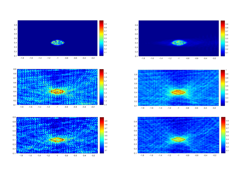
Fig. 4: Reconstruction of a rhombus shaped obstacle shown with a solid black line. The abscissa is range and the ordinate is cross-range, scaled by $|\mathcal{X}|$. Full aperture, noiseless array data. Top line: $\mathcal{J}_{\#}(\vec{{{\itbf z}}})$ . Middle line: $\mathcal{J}_{{\rm mig}\#}(\vec{{{\itbf z}}})$. Bottom line: $\mathcal{J}_{{\rm mig}}(\vec{{{\itbf z}}})$. Left column: 30 propagating modes. Right column: 50 propagating modes.

The robustness to noise is illustrated in Figures 5 and 6, where we display images of a rhombus shaped obstacle and two circle shaped obstacles obtained with noiseless data (left columns) and data contaminated with $\sigma_{\rm noise}=10\%$ noise (right columns).

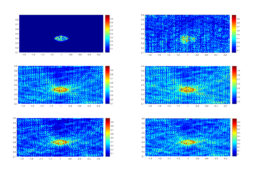
Fig. 5: Reconstruction of a rhombus shaped obstacle shown with a solid black line. The abscissa is range and the ordinate is cross-range, scaled by $|\mathcal{X}|$. Full aperture array data and $30$ propagating modes. Top line: $\mathcal{J}_{\#}(\vec{{{\itbf z}}})$ . Middle line: $\mathcal{J}_{{\rm mig}\#}(\vec{{{\itbf z}}})$. Bottom line: $\mathcal{J}_{{\rm mig}}(\vec{{{\itbf z}}})$. Left column: no noise. Right column: $10\%$ noise.

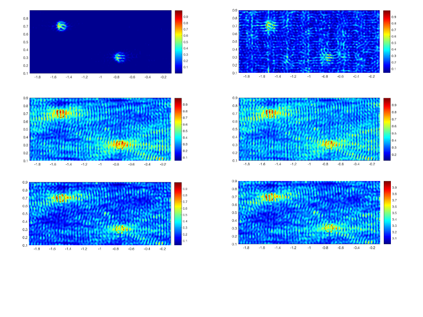
Fig. 6: Reconstruction of two obstacles. The abscissa is range and the ordinate is cross-range, scaled by $|\mathcal{X}|$. Full aperture array data and $30$ propagating modes. Top line: $\mathcal{J}_{\#}(\vec{{{\itbf z}}})$ . Middle line: $\mathcal{J}_{{\rm mig}\#}(\vec{{{\itbf z}}})$. Bottom line: $\mathcal{J}_{{\rm mig}}(\vec{{{\itbf z}}})$. Left column: no noise. Right column: $10\%$ noise.

In the noiseless case, the results in Figures 4–6 show that the factorization method gives better images, as expected from the discussion at the end of section 4.3. However, the migration images are most robust to noise i.e., they are similar for noiseless and the noisy data. Moreover, they improve significantly when we use multifrequency data, as illustrated in Figure 7.

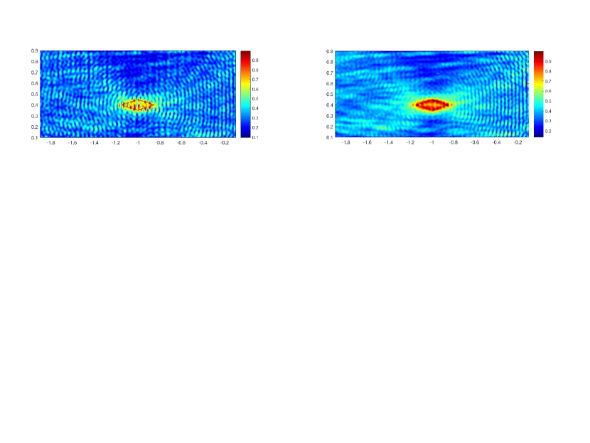
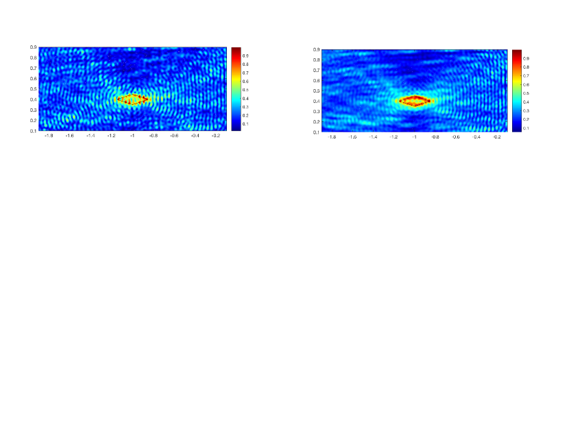
Fig. 7: Reconstruction of a rhombus shaped obstacle shown with a solid black line. The abscissa is range and the ordinate is cross-range, scaled by $|\mathcal{X}|$. Full aperture, noiseless array data and $30$ propagating modes. Top line: $\mathcal{J}_{{\rm mig}\#}(\vec{{{\itbf z}}})$. Bottom line: $\mathcal{J}_{{\rm mig}}(\vec{{{\itbf z}}})$. Single frequency result (left) and multiple frequency result (right).

The last images, in Figure 8 show the effect of the limited array aperture. They are obtained with $30$ propagating modes for noiseless data collected on an array of $|\mathcal{X}|_{{A}}=0.75|\mathcal{X}|$ aperture. The images deteriorate at partial aperture, but the migration method is clearly better when we use the multifrequency data.

Fig. 8: Reconstruction of a rhombus shaped obstacle shown with a solid black line. The abscissa is range and the ordinate is cross-range, scaled by $|\mathcal{X}|$. Noiseless array data. Top line: $\mathcal{J}_{\#}(\vec{{{\itbf z}}})$ . Middle line: $\mathcal{J}_{{\rm mig}\#}(\vec{{{\itbf z}}})$. Bottom line: $\mathcal{J}_{{\rm mig}_{\#}}(\vec{{{\itbf z}}})$ with multifrequency data. Left column: full aperture. Right column: $75\%$ aperture array.

6 Summary

We presented a theoretical and computational comparative study of two qualitative methods for imaging obstacles in a terminating waveguide. The first method is based on the factorization of the far field operator, defined by measurements of the scattered wave collected by an active array of sensors. It is designed to image at a single frequency and determines the support of the obstacles by either solving an optimization problem or, equivalently, using a Picard range criterium. The second method, known as migration, is based on the backpropagation of the measured scattered wave to imaging points, using the Green’s function in the empty waveguide. We studied the classic migration imaging method and explained how to modify it to get better images. Then, we related the migration type imaging method to the factorization method, and compared their performance with numerical simulations.

Appendix A Proof of Lemma 2

Consider first a function $\phi\in L^{2}({A})$ of the form

$$\phi(\vec{{{\itbf x}}})=\sum_{j=0}^{J}\frac{\alpha_{j}}{i}\psi_{j}({{\itbf x}}^{\perp})e^{i\beta_{j}x_{{A}}}+\sum_{j>J}\alpha_{j}\psi_{j}({{\itbf x}}^{\perp}),\qquad\vec{{{\itbf x}}}\in{A},$$ (A.72)

with real valued coefficients $\alpha_{j}$, for $j\geq 0$, and note from the expression (2.11) of the Green’s function and the orthogonality relation (2.7) that

$$\int_{{A}}dS_{\vec{{{\itbf y}}}}\,G(\vec{{{\itbf x}}},\vec{{{\itbf y}}})\phi(\vec{{{\itbf y}}}) =\sum_{j=0}^{J}\frac{\alpha_{j}}{\beta_{j}}\psi_{j}({{\itbf x}}^{\perp})\cos(\beta_{j}x)+\sum_{j>J}\frac{\alpha_{j}}{|\beta_{j}|}\psi_{j}({{\itbf x}}^{\perp})\cosh(|\beta_{j}|x)$$

$$=\int_{{A}}dS_{\vec{{{\itbf y}}}}\,\overline{G(\vec{{{\itbf x}}},\vec{{{\itbf y}}})\phi(\vec{{{\itbf y}}})},\qquad\vec{{{\itbf x}}}\in\partial\Omega.$$ (A.73)

Let us define,

$$w(\vec{{{\itbf x}}}) =\int_{{A}}dS_{\vec{{{\itbf y}}}}\,u^{\rm sc}(\vec{{{\itbf x}}},\vec{{{\itbf y}}})\phi(\vec{{{\itbf y}}}),\qquad\vec{{{\itbf x}}}\in{W}\setminus\overline{\Omega},$$ (A.74)

$$v(\vec{{{\itbf x}}}) =\int_{{A}}dS_{\vec{{{\itbf y}}}}\,\overline{u^{\rm sc}(\vec{{{\itbf x}}},\vec{{{\itbf y}}})\phi(\vec{{{\itbf y}}})},\qquad\vec{{{\itbf x}}}\in{W}\setminus\overline{\Omega},$$ (A.75)

and obtain from (2.12–2.14) and definitions (3.23–3.25) that

$$v,w \in\mathscr{H}(W\setminus\overline{\Omega}),$$ (A.76)

$$w|_{{A}} \in\mathscr{H}^{\rm out}({A}),$$ (A.77)

$$v|_{{A}} \in\mathscr{H}^{\rm in}({A}).$$ (A.78)

Since $u^{\rm sc}(\cdot,\vec{{{\itbf x}}}_{s})|_{\partial\Omega}=-G(\cdot,\vec{{{\itbf x}}}_{s})|_{\partial\Omega}$, we also conclude from (A.73–A.75) that

$$w(\vec{{{\itbf x}}})=v(\vec{{{\itbf x}}}),\qquad\vec{{{\itbf x}}}\in\partial\Omega.$$ (A.79)

At the array, we have by definitions (3.15) and (A.74) that

$$w(\vec{{{\itbf x}}})=\mathcal{N}\phi(\vec{{{\itbf x}}}),\qquad\vec{{{\itbf x}}}\in{A}.$$ (A.80)

Moreover, definition (3.28) and equation (A.79) give

$$v(\vec{{{\itbf x}}})=\mathcal{S}^{-1}w(\vec{{{\itbf x}}})=\mathcal{S}^{-1}\mathcal{N}\phi(\vec{{{\itbf x}}})=\mathcal{F}\phi(\vec{{{\itbf x}}}),\qquad\vec{{{\itbf x}}}\in{A}.$$ (A.81)

This proves that for $\phi$ given in (A.72), we have

$$\mathcal{F}\phi(\vec{{{\itbf x}}})=\int_{{A}}dS_{\vec{{{\itbf y}}}}\,\overline{u^{\rm sc}(\vec{{{\itbf x}}},\vec{{{\itbf y}}})\phi(\vec{{{\itbf y}}})},\qquad\vec{{{\itbf x}}}\in{A}.$$ (A.82)

It remains to prove the result for functions

$$\phi(\vec{{{\itbf x}}})=\phi^{(1)}(\vec{{{\itbf x}}})+i\phi^{(2)}(\vec{{{\itbf x}}}),\qquad\vec{{{\itbf x}}}\in{A},$$

with $\phi^{(l)}$ defined in (3.32). These have the same expression as (A.72), so we write directly from (A.82) that

$$\mathcal{F}\phi^{(l)}(\vec{{{\itbf x}}})=\int_{{A}}dS_{\vec{{{\itbf y}}}}\,\overline{u^{\rm sc}(\vec{{{\itbf x}}},\vec{{{\itbf y}}})\phi^{(l)}(\vec{{{\itbf y}}})},\qquad\vec{{{\itbf x}}}\in{A},~{}~{}l=1,2.$$

Because $\phi^{(l)}$ satisfy equation (A.73), for $l=1,2$, we have that

$$\int_{{A}}dS_{\vec{{{\itbf y}}}}\,G(\vec{{{\itbf x}}},\vec{{{\itbf y}}})\big{[}\phi^{(1)}(\vec{{{\itbf y}}})+i\phi^{(2)}(\vec{{{\itbf y}}})\big{]}=\int_{{A}}dS_{\vec{{{\itbf y}}}}\,\overline{G(\vec{{{\itbf x}}},\vec{{{\itbf y}}})\big{[}\phi^{(1)}(\vec{{{\itbf y}}})-i\phi^{(2)}(\vec{{{\itbf y}}})\big{]}},\qquad\vec{{{\itbf x}}}\in\partial\Omega.$$

Then, the analogues of (A.74–A.75),

$$w(\vec{{{\itbf x}}}) =\int_{{A}}dS_{\vec{{{\itbf y}}}}\,u^{\rm sc}(\vec{{{\itbf x}}},\vec{{{\itbf y}}})\big{[}\phi^{(1)}(\vec{{{\itbf y}}})+i\phi^{(2)}(\vec{{{\itbf y}}})\big{]},\qquad\vec{{{\itbf x}}}\in{W}\setminus\overline{\Omega},$$

$$v(\vec{{{\itbf x}}}) =\int_{{A}}dS_{\vec{{{\itbf y}}}}\,\overline{u^{\rm sc}(\vec{{{\itbf x}}},\vec{{{\itbf y}}})\big{[}\phi^{(1)}(\vec{{{\itbf y}}})-i\phi^{(2)}(\vec{{{\itbf y}}})\big{]}},\qquad\vec{{{\itbf x}}}\in{W}\setminus\overline{\Omega},$$

satisfy (A.76–A.79), and we conclude as above that

$$v(\vec{{{\itbf x}}})=\mathcal{S}^{-1}w(\vec{{{\itbf x}}})=\mathcal{S}^{-1}\mathcal{N}\phi(\vec{{{\itbf x}}})=\mathcal{F}\phi(\vec{{{\itbf x}}})=\mathcal{F}\phi^{(1)}(\vec{{{\itbf x}}})+i\mathcal{F}\phi^{(2)}(\vec{{{\itbf x}}}),\qquad\vec{{{\itbf x}}}\in{A}.$$

This proves Lemma 2. $\Box$

Appendix B Proof of Theorem 3

We begin in section B.1 with the proof of (3.39). The proofs of statements (i) and (ii) of the theorem are in sections B.2 and B.3. We use throughout the appendix the notation

$${W}_{A}^{+}=(x_{A},0)\times\mathcal{X}~{}~{}\mbox{and}~{}~{}{W}_{A}^{-}=(-\infty,x_{A})\times\mathcal{X}.$$

B.1 The factorization of $\mathcal{N}$

Consider the operator $\mathcal{M}:H^{\frac{1}{2}}(\partial\Omega)\to L^{2}({A})$, defined by

$$\mathcal{M}f(\vec{{{\itbf x}}})=w(\vec{{{\itbf x}}}),\qquad\vec{{{\itbf x}}}\in{A},~{}~{}\forall\,f\in H^{\frac{1}{2}}(\partial\Omega),$$ (B.83)

where $w\in\mathscr{H}(W\setminus\overline{\Omega})$ satisfies the outgoing radiation condition at range $x<x_{\Omega}$ and the boundary condition

$$w(\vec{{{\itbf x}}})=-f(\vec{{{\itbf x}}}),\qquad\vec{{{\itbf x}}}\in\partial\Omega.$$ (B.84)

By the definition of $u^{\rm sc}(\vec{{{\itbf x}}},\vec{{{\itbf y}}})$ and using $f=G(\cdot,\vec{{{\itbf y}}})$ in (B.84), we have

$$u^{\rm sc}(\vec{{{\itbf x}}},\vec{{{\itbf y}}})=\big{[}\mathcal{M}G(\cdot,\vec{{{\itbf y}}})|_{\partial\Omega}\big{]}(\vec{{{\itbf x}}}),\qquad\vec{{{\itbf x}}}\in{A}.$$

Therefore, definitions (3.15–3.16) and the linearity of $\mathcal{M}$ give

$$\mathcal{N}g(\vec{{{\itbf x}}}) =\int_{{A}}dS_{\vec{{{\itbf y}}}}\big{[}\mathcal{M}G(\cdot,\vec{{{\itbf y}}})|_{\partial\Omega}\big{]}(\vec{{{\itbf x}}})g(\vec{{{\itbf y}}})=\mathcal{M}\Big{[}\int_{{A}}dS_{\vec{{{\itbf y}}}}G(\cdot,\vec{{{\itbf y}}})|_{\partial\Omega}g(\vec{{{\itbf y}}})\Big{]}(\vec{{{\itbf x}}})$$

$$=\mathcal{M}\mathcal{T}g(\vec{{{\itbf x}}}),\qquad\vec{{{\itbf x}}}\in{A},~{}~{}\forall\,g\in L^{2}({A}).$$

This proves the factorization

$$\mathcal{N}=\mathcal{M}\mathcal{T}.$$ (B.85)

It remains to prove that

$${\mathcal{S}^{-1}\mathcal{M}=\mathcal{T}^{\star}\Lambda.}$$ (B.86)

Take any $f\in H^{\frac{1}{2}}(\partial\Omega)$ and use it to define $h\in H^{-\frac{1}{2}}(\partial\Omega)$ by

$$h(\vec{{{\itbf x}}})=\Lambda f(\vec{{{\itbf x}}}),\qquad\vec{{{\itbf x}}}\in\partial\Omega.$$

With this $h$, we obtain from definition (3.17) that

$$\mathcal{T}^{\star}h(\vec{{{\itbf x}}})=\mathcal{T}^{\star}\Lambda f(\vec{{{\itbf x}}})=\int_{\partial\Omega}dS_{\vec{{{\itbf z}}}}\,\overline{G(\vec{{{\itbf z}}},\vec{{{\itbf x}}})}h(\vec{{{\itbf z}}}),\qquad\vec{{{\itbf x}}}\in{A}.$$

If we let $v\in\mathscr{H}(W\setminus\overline{\Omega})$ be defined by

$$v(\vec{{{\itbf x}}})=\int_{\partial\Omega}dS_{\vec{{{\itbf z}}}}\,\overline{G(\vec{{{\itbf z}}},\vec{{{\itbf x}}})}h(\vec{{{\itbf z}}}),\qquad\vec{{{\itbf x}}}\in{W}\setminus\overline{\Omega},$$ (B.87)

then we have

$$v(\vec{{{\itbf x}}}) =\mathcal{T}^{\star}\Lambda f(\vec{{{\itbf x}}}),\qquad\vec{{{\itbf x}}}\in{A},$$ (B.88)

$$v(\vec{{{\itbf x}}}) =-f(\vec{{{\itbf x}}}),\qquad\vec{{{\itbf x}}}\in\partial\Omega,$$ (B.89)

where (B.89) is obtained from definition (3.21). We also have that $v|_{{A}}\in\mathscr{H}^{in}({A}),$ so we can define

$${\mathcal{S}^{-1}w(\vec{{{\itbf x}}})=v(\vec{{{\itbf x}}})=\mathcal{T}^{\star}\Lambda f(\vec{{{\itbf x}}})},\qquad\vec{{{\itbf x}}}\in{A}.$$

The factorization (B.86) follows from this equation, definition (3.28) of $\mathcal{S}^{-1}$, equation (B.89) and definition (B.83) of $\mathcal{M}$, which give

$$w(\vec{{{\itbf x}}})=\mathcal{M}f(\vec{{{\itbf x}}}),\qquad\vec{{{\itbf x}}}\in{A}.$$

$\Box$

B.2 Proof of statement (i)

Consider the operator $\widetilde{\mathcal{T}}:H^{-\frac{1}{2}}({A})\to H^{\frac{1}{2}}(\partial\Omega)$,

$$\widetilde{\mathcal{T}}g(\vec{{{\itbf z}}})=\int_{{A}}dS_{\vec{{{\itbf y}}}}\,G(\vec{{{\itbf z}}},\vec{{{\itbf y}}})g(\vec{{{\itbf y}}}),\qquad\forall\,\vec{{{\itbf z}}}\in\partial\Omega,~{}~{}\forall\,g\in L^{2}({A}).$$ (B.90)

whose restriction to the domain $L^{2}({A})\subset H^{-\frac{1}{2}}({A})$ is the operator $\mathcal{T}$ defined in (3.16).

B.2.1 Proof that $\widetilde{\mathcal{T}}$ is bounded

The Green’s function $G(\vec{{{\itbf z}}},\vec{{{\itbf x}}})$ is smooth for $\vec{{{\itbf z}}}\neq\vec{{{\itbf x}}}$, so

$$v(\vec{{{\itbf z}}})=\int_{{A}}dS_{\vec{{{\itbf x}}}}\,G(\vec{{{\itbf z}}},\vec{{{\itbf x}}})g(\vec{{{\itbf x}}})\in H^{1}\big{(}{W}_{{A}}^{+}\big{)},\qquad\forall\,g\in H^{-\frac{1}{2}}({A}).$$

Moreover, for $\vec{{{\itbf z}}}\in\Omega$,

$$\Delta_{\vec{{{\itbf z}}}}v(\vec{{{\itbf z}}})=\int_{{A}}dS_{\vec{{{\itbf x}}}}\,\Delta_{\vec{{{\itbf z}}}}G(\vec{{{\itbf z}}},\vec{{{\itbf x}}})g(\vec{{{\itbf x}}})=-k^{2}\int_{{A}}dS_{\vec{{{\itbf x}}}}\,G(\vec{{{\itbf z}}},\vec{{{\itbf x}}})g(\vec{{{\itbf x}}})=-k^{2}v(\vec{{{\itbf z}}}).$$

By the mapping property of the single layer potential, $\|v\|_{H^{1}\big{(}\Omega\big{)}}\leq C_{1}\|g\|_{H^{-\frac{1}{2}}(\partial\Omega)}$ for some constant $C_{1}>0$, which gives

$$\|\Delta_{\vec{{{\itbf z}}}}v(\vec{{{\itbf z}}})\|_{L^{2}(\Omega)}\leq k^{2}\|v(\vec{{{\itbf z}}})\|_{L^{2}(\Omega)}\leq C_{2}\|g\|_{H^{-\frac{1}{2}}(\partial\Omega)},$$

for another constant $C_{2}>0$. Then, we obtain from [35, Lemma 4.3] that

$$\widetilde{\mathcal{T}}g=v|_{\partial\Omega}\in H^{\frac{1}{2}}(\partial\Omega)~{}~{}\mbox{and}~{}~{}\|\widetilde{\mathcal{T}}g\|_{H^{\frac{1}{2}}(\partial\Omega)}\leq C\|g\|_{H^{-\frac{1}{2}}(\partial\Omega)},$$ (B.91)

for yet another constant $C>0$, so $\widetilde{\mathcal{T}}$ is bounded.

B.2.2 Proof that $\mathcal{T}$ is compact

Consider any bounded sequence in $L^{2}({A})$, which must have a weakly convergent subsequence $\{g_{n}\}$ with weak limit $g\in L^{2}({A})$. Because $L^{2}({A})$ is compactly embedded in $H^{-\frac{1}{2}}({A})$, this sequence converges strongly in $H^{-\frac{1}{2}}({A})$,

$$\lim_{n\to\infty}\|g_{n}-g\|_{H^{-\frac{1}{2}}({A})}=0.$$ (B.92)

Recalling that $\mathcal{T}$ is the restriction of $\widetilde{\mathcal{T}}$ to the domain $L^{2}({A})$, we have

$$\mathcal{T}g_{n}=\widetilde{\mathcal{T}}g_{n}~{}~{}\mbox{and}~{}~{}\mathcal{T}g=\widetilde{\mathcal{T}}g,$$

and using (B.91),

$$\|\mathcal{T}g_{n}-\mathcal{T}g\|_{H^{\frac{1}{2}}(\partial\Omega)}=\|\widetilde{\mathcal{T}}g_{n}-\widetilde{\mathcal{T}}g\|_{H^{\frac{1}{2}}(\partial\Omega)}\leq C\|g_{n}-g\|_{H^{-\frac{1}{2}}({A})}.$$ (B.93)

We conclude from (B.92–B.93) that $\{\mathcal{T}g_{n}\}$ converges to $\mathcal{T}g$, strongly in $H^{\frac{1}{2}}(\partial\Omega)$. This proves that $\mathcal{T}$ is compact.

B.2.3 Proof that $\mathcal{T}$ is injective

Let us define

$$v(\vec{{{\itbf z}}})=\int_{{A}}dS_{\vec{{{\itbf x}}}}\,G(\vec{{{\itbf z}}},\vec{{{\itbf x}}})g(\vec{{{\itbf x}}}),\qquad\vec{{{\itbf z}}}\in{W},$$ (B.94)

where $g$ satisfies

$$v(\vec{{{\itbf z}}})=\mathcal{T}g(\vec{{{\itbf z}}})=0,\qquad\vec{{{\itbf z}}}\in\partial\Omega.$$ (B.95)

To prove injectivity, we must show that $g=0$.

Equations (B.94–B.95) give

$$(\Delta_{\vec{{{\itbf z}}}}+k^{2})v(\vec{{{\itbf z}}}) =0,\qquad\vec{{{\itbf z}}}\in\Omega,$$

$$v(\vec{{{\itbf z}}}) =0,\qquad\vec{{{\itbf z}}}\in\partial\Omega,$$

and by Assumption 2,

$$v(\vec{{{\itbf z}}})=0,\qquad\forall\,\vec{{{\itbf z}}}\in\overline{\Omega}.$$

Since $v$ is analytic at $\vec{{{\itbf z}}}\in(x_{{A}},0)\times\mathcal{X}$, we obtain by unique continuation that

$$v(\vec{{{\itbf z}}})=0,\qquad\forall\,\vec{{{\itbf z}}}\in{W}_{{A}}^{+}\cup{A}.$$

On the left of the array, we have

$$(\Delta_{\vec{{{\itbf z}}}}+k^{2})v(\vec{{{\itbf z}}}) =0,\qquad\vec{{{\itbf z}}}\in{W}_{{A}}^{-},$$

$$v(\vec{{{\itbf z}}}) =0,\qquad\vec{{{\itbf z}}}\in{A},$$

$$\partial_{\vec{\bm{\nu}}_{\vec{{{\itbf z}}}}}v(\vec{{{\itbf z}}}) =0,\qquad\vec{{{\itbf z}}}\in\partial{W},$$

and $v$ satisfies the outgoing radiation condition at range $x<x_{{A}}$. By the uniqueness of solution (see for example [9, Lemma A.2])

$$v(\vec{{{\itbf z}}})=0,\qquad\forall\,\vec{{{\itbf z}}}\in{W}_{{A}}^{-}.$$

But (B.94) is a single layer potential, satisfying the jump condition

$${-g|_{{A}}}=[\partial_{\vec{\bm{\nu}}}v]\big{|}_{{A}}=0,$$

where $[\cdot]\big{|}_{{A}}$ denotes the jump at ${A}$. This proves that $\mathcal{T}$ is injective. $\Box$

B.3 Proof of statement (ii)

We show first that ${-\mathscr{I}(\Lambda)}$ is positive semi-definite and then we prove the result on $\mathscr{R}(\Lambda)$.

B.3.1 The operator $\Im(\Lambda)$

Recall definition (3.21) and introduce the functions

$$h(\vec{{{\itbf x}}})=\Lambda f(\vec{{{\itbf x}}})~{}~{}\mbox{and}~{}~{}\widetilde{h}(\vec{{{\itbf x}}})=\Lambda\widetilde{f}(\vec{{{\itbf x}}}),\qquad\vec{{{\itbf x}}}\in\partial\Omega,$$ (B.96)

for arbitrary $f,\widetilde{f}\in H^{\frac{1}{2}}(\partial\Omega)$, where $h\in H^{-\frac{1}{2}}(\partial\Omega)$ is the unique solution of

$$\int_{\partial\Omega}dS_{\vec{{{\itbf y}}}}\,\overline{G(\vec{{{\itbf x}}},\vec{{{\itbf y}}})}\,h(\vec{{{\itbf y}}})=-f(\vec{{{\itbf x}}}),\qquad\vec{{{\itbf x}}}\in\partial\Omega,$$ (B.97)

and $\widetilde{h}$ satisfies a similar equation, with $\widetilde{f}$ in the right hand side. Define

$$v(\vec{{{\itbf x}}}) =\int_{\partial\Omega}dS_{\vec{{{\itbf y}}}}\,\overline{G(\vec{{{\itbf x}}},\vec{{{\itbf y}}})}\,h(\vec{{{\itbf y}}}),\qquad\vec{{{\itbf x}}}\in{W}\setminus\partial\Omega,$$ (B.98)

$$\widetilde{v}(\vec{{{\itbf x}}}) =\int_{\partial\Omega}dS_{\vec{{{\itbf y}}}}\,\overline{G(\vec{{{\itbf x}}},\vec{{{\itbf y}}})}\,\widetilde{h}(\vec{{{\itbf y}}}),\qquad\vec{{{\itbf x}}}\in{W}\setminus\partial\Omega,$$ (B.99)

and note that (B.97) implies

$$v(\vec{{{\itbf x}}})=-f(\vec{{{\itbf x}}})~{}~{}\mbox{and}~{}~{}\widetilde{v}(\vec{{{\itbf x}}})=-\widetilde{f}(\vec{{{\itbf x}}}),\qquad\vec{{{\itbf x}}}\in\partial\Omega.$$ (B.100)

Since (B.98–B.99) are single layer potentials, we have from [35, Theorem 6.11]

$${-h}\big{|}_{\partial\Omega}=[\partial_{\vec{\bm{\nu}}}v]\big{|}_{\partial\Omega}~{}~{}\mbox{and}~{}~{}{-\widetilde{h}}\big{|}_{\partial\Omega}=[\partial_{\vec{\bm{\nu}}}\widetilde{v}]\big{|}_{\partial\Omega},$$ (B.101)

where $[\cdot]$ denotes the jump at $\partial\Omega$.

These results imply that

$${-}\left<\Lambda f,\widetilde{f}\right>_{\partial\Omega} ={-}\left<h,\widetilde{f}\right>_{\partial\Omega}={-}\int_{\partial\Omega}dS_{\vec{{{\itbf x}}}}\,\overline{h(\vec{{{\itbf x}}})}\,\widetilde{f}(\vec{{{\itbf x}}})=\int_{\partial\Omega}dS_{\vec{{{\itbf x}}}}\,\overline{h(\vec{{{\itbf x}}})}\,\widetilde{v}(\vec{{{\itbf x}}}),$$

$$=-\int_{\partial\Omega}dS_{\vec{{{\itbf x}}}}\,\big{[}\overline{\partial_{\vec{\bm{\nu}}_{{}_{\vec{{{\itbf x}}}}}}v^{+}(\vec{{{\itbf x}}})}-\overline{\partial_{\vec{\bm{\nu}}_{{}_{\vec{{{\itbf x}}}}}}v^{-}(\vec{{{\itbf x}}})}\big{]}\widetilde{v}(\vec{{{\itbf x}}}),$$ (B.102)

with indexes $\pm$ denoting the function $v$ outside or inside $\Omega$. Using the identity

$$\nabla_{\vec{{{\itbf x}}}}\cdot\big{[}\widetilde{v}(\vec{{{\itbf x}}})\nabla_{\vec{{{\itbf x}}}}\overline{v^{\pm}(\vec{{{\itbf x}}})}\big{]} =\widetilde{v}(\vec{{{\itbf x}}})\Delta_{\vec{{{\itbf x}}}}\overline{v^{\pm}(\vec{{{\itbf x}}})}+\nabla_{\vec{{{\itbf x}}}}\widetilde{v}(\vec{{{\itbf x}}})\cdot\nabla_{\vec{{{\itbf x}}}}\overline{v^{\pm}(\vec{{{\itbf x}}})}$$

$$=-k^{2}\widetilde{v}(\vec{{{\itbf x}}})\overline{v^{\pm}(\vec{{{\itbf x}}})}+\nabla_{\vec{{{\itbf x}}}}\widetilde{v}(\vec{{{\itbf x}}})\cdot\nabla_{\vec{{{\itbf x}}}}\overline{v^{\pm}(\vec{{{\itbf x}}})},$$

and integration by parts, we obtain that

$$\int_{{W}_{{A}}^{+}\setminus\overline{\Omega}}d\vec{{{\itbf x}}}\Big{[}-k^{2}\widetilde{v}(\vec{{{\itbf x}}})\overline{v^{+}(\vec{{{\itbf x}}})}+\nabla_{\vec{{{\itbf x}}}}\widetilde{v}(\vec{{{\itbf x}}})\cdot\nabla_{\vec{{{\itbf x}}}}\overline{v^{+}(\vec{{{\itbf x}}})}\Big{]} =-\int_{{A}}dS_{\vec{{{\itbf x}}}}\,\widetilde{v}(\vec{{{\itbf x}}})\overline{\partial_{\vec{\bm{\nu}}_{{}_{\vec{{{\itbf x}}}}}}v^{+}(\vec{{{\itbf x}}})}$$

$$-\int_{\partial\Omega}dS_{\vec{{{\itbf x}}}}\,\widetilde{v}(\vec{{{\itbf x}}})\overline{\partial_{\vec{\bm{\nu}}_{{}_{\vec{{{\itbf x}}}}}}v^{+}(\vec{{{\itbf x}}})},$$

and

$$\int_{\Omega}d\vec{{{\itbf x}}}\Big{[}-k^{2}\widetilde{v}(\vec{{{\itbf x}}})\overline{v^{-}(\vec{{{\itbf x}}})}+\nabla_{\vec{{{\itbf x}}}}\widetilde{v}(\vec{{{\itbf x}}})\cdot\nabla_{\vec{{{\itbf x}}}}\overline{v^{-}(\vec{{{\itbf x}}})}= \int_{\partial\Omega}dS_{\vec{{{\itbf x}}}}\,\widetilde{v}(\vec{{{\itbf x}}})\overline{\partial_{\vec{\bm{\nu}}_{{}_{\vec{{{\itbf x}}}}}}v^{-}(\vec{{{\itbf x}}})}.$$

Substituting these equations in (B.102) we get

$${-}\left<\Lambda f,\widetilde{f}\right>_{\partial\Omega}= \int_{{A}}dS_{\vec{{{\itbf x}}}}\,\widetilde{v}(\vec{{{\itbf x}}})\overline{\partial_{\vec{\bm{\nu}}_{{}_{\vec{{{\itbf x}}}}}}v(\vec{{{\itbf x}}})}+\int_{{W}_{{A}}^{+}\setminus\partial\Omega}d\vec{{{\itbf x}}}\Big{[}-k^{2}\widetilde{v}(\vec{{{\itbf x}}})\overline{v(\vec{{{\itbf x}}})}+\nabla_{\vec{{{\itbf x}}}}\widetilde{v}(\vec{{{\itbf x}}})\cdot\nabla_{\vec{{{\itbf x}}}}\overline{v(\vec{{{\itbf x}}})}\Big{]},$$ (B.103)

where we droped the $\pm$ indexes on $v$. The same calculation, with $v$ and $\widetilde{v}$ interchanged, gives

$${-}\left<\widetilde{f},\Lambda^{\star}f\right>_{\partial\Omega}= {-}\left<\Lambda\widetilde{f},f\right>_{\partial\Omega}=\int_{{A}}dS_{\vec{{{\itbf x}}}}\,{v}(\vec{{{\itbf x}}})\overline{\partial_{\vec{\bm{\nu}}_{{}_{\vec{{{\itbf x}}}}}}\widetilde{v}(\vec{{{\itbf x}}})}$$

$$+\int_{{W}_{{A}}^{+}\setminus\partial\Omega}\Big{[}-k^{2}v(\vec{{{\itbf x}}})\overline{\widetilde{v}^{(}\vec{{{\itbf x}}})}+\nabla_{\vec{{{\itbf x}}}}v(\vec{{{\itbf x}}})\cdot\nabla_{\vec{{{\itbf x}}}}\overline{\widetilde{v}(\vec{{{\itbf x}}})}={-}\overline{\left<\Lambda^{\star}f,\widetilde{f}\right>_{\partial\Omega}}.$$ (B.104)

Therefore, $\Im(\Lambda)=\big{(}\Lambda-\Lambda^{\star}\big{)}/(2i)$ satisfies

$${-}\left<\Im(\Lambda)f,\widetilde{f}\right>_{\partial\Omega}=-\frac{1}{2i}\int_{{A}}dS_{\vec{{{\itbf x}}}}\Big{[}\widetilde{v}(\vec{{{\itbf x}}})\overline{\partial_{\vec{\bm{\nu}}_{{}_{\vec{{{\itbf x}}}}}}v(\vec{{{\itbf x}}})}-\overline{v(\vec{{{\itbf x}}})}\partial_{\vec{\bm{\nu}}_{{}_{\vec{{{\itbf x}}}}}}\widetilde{v}(\vec{{{\itbf x}}})\Big{]}.$$ (B.105)

We can write (B.105) more explicitly using the expression (2.11) of the Green’s function in the definitions (B.98–B.99) of $v$ and $\widetilde{v}$. We obtain

$$v(\vec{{{\itbf x}}}) =\sum_{j=0}^{\infty}\psi_{j}({{\itbf x}}^{\perp})v_{j}$$ (B.106)

$$\partial_{\vec{\bm{\nu}}_{{}_{\vec{{{\itbf x}}}}}}v(\vec{{{\itbf x}}}) =\sum_{j=0}^{J}i\beta_{j}\psi_{j}({{\itbf x}}^{\perp})v_{j}+\sum_{j>J}|\beta_{j}|\psi_{j}({{\itbf x}}^{\perp})v_{j},\qquad\vec{{{\itbf x}}}\in{A},$$ (B.107)

where

$$v_{j}=\left\{\begin{array}[]{ll}-\frac{i}{\beta_{j}}\int_{\partial\Omega}dS_{\vec{{{\itbf y}}}}\,h(\vec{{{\itbf y}}})\psi_{j}({{\itbf y}}^{\perp})e^{i\beta_{j}x_{{A}}}\cos(\beta_{j}y),&j=0,\ldots,J,\\ \\ \frac{1}{|\beta_{j}|}\int_{\partial\Omega}dS_{\vec{{{\itbf y}}}}\,h(\vec{{{\itbf y}}})\psi_{j}({{\itbf y}}^{\perp})e^{|\beta_{j}|x_{{A}}}\cosh(|\beta_{j}|y),&j>J,\end{array}\right.$$ (B.108)

and similar for $\widetilde{v}$. Substituting in (B.107) and using the orthogonality relation (2.7),

$${-}\left<\Im(\Lambda)f,\widetilde{f}\right>_{\partial\Omega}=\sum_{j=0}^{J}\beta_{j}\widetilde{v}_{j}\overline{v_{j}}.$$ (B.109)

In particular, for $\widetilde{f}=f$,

$${-}\left<\Im(\Lambda)f,f\right>_{\partial\Omega}=\sum_{j=0}^{J}\beta_{j}|v_{j}|^{2}\geq 0,\qquad\forall\,f\in H^{\frac{1}{2}}(\partial\Omega).$$ (B.110)

This proves that $-\Im(\Lambda)$ is positive semi-definite. $\Box$

B.3.2 The operator $\mathscr{R}(\Lambda)$

We introduce the operator $\Lambda_{i}$ by

$$h(\vec{{{\itbf x}}})=\Lambda_{i}f(\vec{{{\itbf x}}}),\qquad\vec{{{\itbf x}}}\in\partial\Omega,$$ (B.111)

for arbitrary $f\in H^{\frac{1}{2}}(\partial\Omega)$, where $h\in H^{-\frac{1}{2}}(\partial\Omega)$ is the unique solution of

$$\int_{\partial\Omega}dS_{\vec{{{\itbf y}}}}\,\overline{G_{i}(\vec{{{\itbf x}}},\vec{{{\itbf y}}})}\,h(\vec{{{\itbf y}}})=-f(\vec{{{\itbf x}}}),\qquad\vec{{{\itbf x}}}\in\partial\Omega,$$ (B.112)

with $G_{i}(\vec{{{\itbf x}}},\vec{{{\itbf y}}})$ the Green function when $k=i$. We let $v_{i}$ satisfy (B.98) with $G(\vec{{{\itbf x}}},\vec{{{\itbf y}}})$ replaced by $G_{i}(\vec{{{\itbf x}}},\vec{{{\itbf y}}})$. By Assumption 2, both $\Lambda$ and $\Lambda_{i}$ have bounded inverses, and from (3.21) – (3.22) we see that for any $h\in H^{-\frac{1}{2}}(\partial\Omega)$,

$$\Lambda^{-1}h(\vec{{{\itbf x}}})=-\int_{\partial\Omega}dS_{\vec{{{\itbf y}}}}\,\overline{G(\vec{{{\itbf x}}},\vec{{{\itbf y}}})}\,h(\vec{{{\itbf y}}}),\qquad\vec{{{\itbf x}}}\in\partial\Omega,$$ (B.113)

The analogue of this equation holds for $\Lambda_{i}^{-1}$ with $G(\vec{{{\itbf x}}},\vec{{{\itbf y}}})$ replaced by $G_{i}(\vec{{{\itbf x}}},\vec{{{\itbf y}}})$.

Note that $G(\vec{{{\itbf x}}},\vec{{{\itbf y}}})-G_{i}(\vec{{{\itbf x}}},\vec{{{\itbf y}}})$ satisfies the Helmoltz equation and it is smooth. In particular, this is so for $\vec{{{\itbf x}}},\vec{{{\itbf y}}}\in\partial\Omega$. Because $\overline{G(\vec{{{\itbf x}}},\vec{{{\itbf y}}})}-\overline{G_{i}(\vec{{{\itbf x}}},\vec{{{\itbf y}}})}$ is the kernel of operator $\Lambda^{-1}-\Lambda_{i}^{-1}$, it follows that $\Lambda^{-1}-\Lambda_{i}^{-1}$ is compact. Furthermore

$$\Lambda-\Lambda_{i}=\Lambda_{i}(\Lambda_{i}^{-1}-\Lambda^{-1})\Lambda$$

is compact and $\mathscr{R}(\Lambda-\Lambda_{i})$ is compact. The representation (B.103) of $\Lambda_{i}$ (where we replace $k$ by $i$) gives $\Lambda_{i}^{*}=\Lambda_{i}$ and

$$-\left<\Lambda_{i}f,f\right>_{\partial\Omega} \geq\|v_{i}\|_{H^{1}({W}_{{A}}^{+}\setminus\partial\Omega)}^{2}\geq C\|f\|_{H^{\frac{1}{2}}(\partial\Omega)},\qquad\forall\,f\in H^{\frac{1}{2}}(\partial\Omega).$$

This yields that $-\mathscr{R}(\Lambda)=-\Lambda_{i}-\mathscr{R}(\Lambda-\Lambda_{i})$ is the sum of a positive definite, self-adjoint operator and a compact operator. $\Box$

Appendix C Proof of Lemma 4

Let us start with the case $\vec{{{\itbf z}}}\in\Omega$. Since $G(\cdot,\vec{{{\itbf z}}})\big{|}_{\partial\Omega}$ is in $H^{\frac{1}{2}}(\partial\Omega)$, we can define $h\in H^{-\frac{1}{2}}(\partial\Omega)$ by

$$h\big{|}_{\partial\Omega}=-\Lambda\,\overline{G(\cdot,\vec{{{\itbf z}}})}\big{|}_{\partial\Omega},$$ (C.114)

where we recall from definition (3.21) that $h$ is the unique solution of

$$\int_{\partial\Omega}dS_{\vec{{{\itbf y}}}}\,G(\vec{{{\itbf x}}},\vec{{{\itbf y}}})\overline{h(\vec{{{\itbf y}}})}=G(\vec{{{\itbf x}}},\vec{{{\itbf z}}}),\qquad\vec{{{\itbf x}}}\in\partial\Omega.$$ (C.115)

With this $h$, let

$$w(\vec{{{\itbf x}}})=\int_{\partial\Omega}dS_{\vec{{{\itbf y}}}}\,G(\vec{{{\itbf x}}},\vec{{{\itbf y}}})\overline{h(\vec{{{\itbf y}}})},\qquad\vec{{{\itbf x}}}\in{W}\setminus\partial\Omega.$$ (C.116)

Then, $v(\vec{{{\itbf x}}})=w(\vec{{{\itbf x}}})-{G(\vec{{{\itbf x}}},\vec{{{\itbf z}}})}$ is in $\mathscr{H}({W}\setminus\overline{\Omega})$ and it satsifies the outgoing radiation condition at range $x<x_{\Omega}$ and the boundary condition $v\big{|}_{\partial\Omega}=0$. By Assumption 1, we conclude that $v(\vec{{{\itbf x}}})=0$ in ${W}\setminus\overline{\Omega}.$ This implies in particular that

$$w(\vec{{{\itbf x}}})=G(\vec{{{\itbf x}}},\vec{{{\itbf z}}}),\qquad\vec{{{\itbf x}}}\in{A}.$$ (C.117)

Furthermore, by definition (3.17), we get for all $\vec{{{\itbf x}}}\in{A}$,

$$\mathcal{T}^{\star}h(\vec{{{\itbf x}}})=\int_{\partial\Omega}dS_{\vec{{{\itbf y}}}}\,\overline{G(\vec{{{\itbf y}}},\vec{{{\itbf x}}})}h(\vec{{{\itbf y}}})=\int_{\partial\Omega}dS_{\vec{{{\itbf y}}}}\,\overline{G(\vec{{{\itbf x}}},\vec{{{\itbf y}}})}h(\vec{{{\itbf y}}})=\overline{w(\vec{{{\itbf x}}})}=\overline{G(\vec{{{\itbf x}}},\vec{{{\itbf z}}})},$$ (C.118)

where we used (C.116), (C.117) and the reciprocity of the Green’s function. This shows that $\overline{G(\cdot,\vec{{{\itbf z}}})}\big{|}_{{A}}\in\mbox{range}(\mathcal{T}^{\star})$.

To prove the converse, suppose that $\vec{{{\itbf z}}}\notin\Omega$ and assume for a contradiction argument that $\overline{G(\cdot,\vec{{{\itbf z}}})}\big{|}_{{A}}\in\mbox{range}(\mathcal{T}^{\star}).$ Then, there exists $h\in H^{-\frac{1}{2}}(\partial\Omega)$ such that

$$\mathcal{T}^{\star}h(\vec{{{\itbf x}}})=\int_{\partial\Omega}dS_{\vec{{{\itbf y}}}}\,\overline{G(\vec{{{\itbf y}}},\vec{{{\itbf x}}})}h(\vec{{{\itbf y}}})=\overline{G(\vec{{{\itbf x}}},\vec{{{\itbf z}}})},\qquad\vec{{{\itbf x}}}\in{A}.$$ (C.119)

This $h$ defines a function $w$ as in (C.116), satisfying $w\in H_{\rm loc}^{1}({W}\setminus\overline{\Omega})$, with trace $w\big{|}_{\partial\Omega}\in H^{\frac{1}{2}}(\partial\Omega)$. If we define further

$$v(\vec{{{\itbf x}}})=w(\vec{{{\itbf x}}})-G(\vec{{{\itbf x}}},\vec{{{\itbf z}}}),$$ (C.120)

then we obtain that it satisfies the boundary value problem

$$(\Delta_{\vec{{{\itbf x}}}}+k^{2})v(\vec{{{\itbf x}}}) =0,\qquad\vec{{{\itbf x}}}\in{W}_{A}^{-},$$

$$\partial_{\vec{\bm{\nu}}_{{}_{\vec{{{\itbf x}}}}}}v(\vec{{{\itbf x}}}) =0,\qquad\vec{{{\itbf x}}}\in\partial{W},$$

$$v(\vec{{{\itbf x}}}) =0,\qquad\vec{{{\itbf x}}}\in{A},$$

and the outgoing radiation condition at $x<x_{{A}}.$ This problem has the unique solution (see for example [9, Lemma A.2])

$$v(\vec{{{\itbf x}}})=0,\qquad\vec{{{\itbf x}}}\in{W}_{{A}}^{-}\cup{A},$$

and since $v$ is analytic at $\vec{{{\itbf x}}}\notin\overline{\Omega}\cup\{\vec{{{\itbf z}}}\}$, we have by unique continuation

$$v(\vec{{{\itbf x}}})=0~{}~{}\mbox{i.e.}~{}~{}w(\vec{{{\itbf x}}})=G(\vec{{{\itbf x}}},\vec{{{\itbf z}}}),\qquad\vec{{{\itbf x}}}\in{W}\setminus\{\overline{\Omega}\cup\{\vec{{{\itbf z}}}\}\}.$$

Then, $w(\vec{{{\itbf x}}})$ blows up, like $G(\vec{{{\itbf x}}},\vec{{{\itbf z}}})$, as $\vec{{{\itbf x}}}\to\vec{{{\itbf z}}}$. This contradicts that $w\in H_{\rm loc}^{1}({W}\setminus\overline{\Omega})$ and $w\big{|}_{\partial\Omega}\in H^{\frac{1}{2}}(\partial\Omega)$. Therefore, $\overline{G(\cdot,\vec{{{\itbf z}}})}\big{|}_{{A}}\notin\mbox{range}(\mathcal{T}^{\star})$ when $\vec{{{\itbf z}}}\notin\Omega$. $\Box$

Appendix D Proof of Theorem 6

To prove the theorem, we begin with two lemmas, proved in sections D.1 and D.2.

Lemma 10.

Denote by $\overline{\mathcal{T}({\mathscr{P}})}$ the closure of the image of the set ${\mathscr{P}}$ defined in (3.49) under the operator $\mathcal{T}$ defined in (3.16). Recall also the sets ${\mathscr{P}}_{0}$ and ${\mathscr{P}}_{0}^{\perp}$ defined in (4.65) and denote by $\mathcal{T}({\mathscr{P}}_{0})$ and $\mathcal{T}({\mathscr{P}}_{0}^{\perp})$ their image under $\mathcal{T}$. We have

$$\left<-\Im(\Lambda)f,f\right>_{\partial\Omega}\neq 0,\qquad\forall\,f\in\overline{\mathcal{T}({\mathscr{P}})},~{}~{}f\notin\mathcal{T}({\mathscr{P}}_{0}),~{}~{}f\neq 0.$$ (D.121)

Moreover, there exists a positive constant $C$ such that

$$\left<-\Im(\Lambda)f,f\right>_{\partial\Omega}\geq C\|f\|^{2}_{H^{\frac{1}{2}}(\partial\Omega)},\qquad\forall\,f\in\mathcal{T}({\mathscr{P}}_{0}^{\perp}),~{}~{}f\neq 0.$$ (D.122)

Lemma 11.

A search point $\vec{{{\itbf z}}}$ lies in $\Omega$ and therefore, by Lemma 4, we have $\overline{G(\cdot,\vec{{{\itbf z}}})}\big{|}_{{A}}\in\mbox{range}(\mathcal{T}^{\star})$, if and only if $\overline{G_{{\mathscr{P}}}(\cdot,\vec{{{\itbf z}}})}\big{|}_{{A}}\in\mbox{range}(\mathcal{T}^{\star})\big{|}_{{\mathscr{P}}}.$

Proof of Theorem 6: By assumption, $\overline{G_{{\mathscr{P}}}(\cdot,\vec{{{\itbf z}}})}\big{|}_{{A}}\notin{\mathscr{P}}_{0}$, so there exists $\varphi\in{\mathscr{P}}_{0}^{\perp}$ so that

$$\big{(}\overline{G_{{\mathscr{P}}}(\cdot,\vec{{{\itbf z}}})},\varphi\big{)}_{{A}}\neq 0.$$

Therefore,

$$\Phi=\{\varphi\in{\mathscr{P}}_{0}^{\perp},~{}~{}\big{(}\overline{G_{{\mathscr{P}}}(\cdot,\vec{{{\itbf z}}})},\varphi\big{)}_{{A}}=1\}\neq\emptyset.$$

Because $\vec{{{\itbf z}}}\in\Omega$, we conclude from Lemma 11 that $\overline{G_{{\mathscr{P}}}(\cdot,\vec{{{\itbf z}}})}\big{|}_{{A}}\in\mbox{range}(\mathcal{T}^{\star})\big{|}_{{\mathscr{P}}}.$ That is to say,

$$\exists\,\theta\in H^{-\frac{1}{2}}(\partial\Omega)~{}~{}\mbox{such that}~{}~{}\overline{G_{{\mathscr{P}}}(\vec{{{\itbf x}}},\vec{{{\itbf z}}})}=\mathbb{P}\mathcal{T}^{\star}\theta(\vec{{{\itbf x}}}),\qquad\vec{{{\itbf x}}}\in{A}.$$

We also have from the factorization of $\mathcal{F}$ in Theorem 3 and definition (3.43) that

$${-\big{(}\Im(\mathcal{F})\varphi,\varphi\big{)}_{{A}}=-\big{(}\mathcal{T}^{\star}\Im(\Lambda)\mathcal{T}\varphi,\varphi\big{)}_{{A}}=-\left<\Im(\Lambda)\mathcal{T}\varphi,\mathcal{T}\varphi\right>_{\partial\Omega}}\geq C\|\mathcal{T}\varphi\|^{2}_{H^{\frac{1}{2}}(\partial\Omega)},$$

for all $\varphi\in\Phi$, where we used the bound (D.122) in Lemma 2. With these results we get

$$C =C\Big{|}\big{(}\overline{G_{{\mathscr{P}}}(\cdot,\vec{{{\itbf z}}})},\varphi\big{)}_{{A}}\Big{|}^{2}=C\Big{|}\big{(}\mathbb{P}\mathcal{T}^{\star}\theta,\varphi\big{)}_{{A}}\Big{|}^{2}=C\Big{|}\big{(}\mathcal{T}^{\star}\theta,\varphi\big{)}_{{A}}\Big{|}^{2}$$

$$=C\Big{|}\left<\theta,\mathcal{T}\varphi\right>_{\partial\Omega}\Big{|}^{2}\leq C\|\theta\|^{2}_{H^{-\frac{1}{2}}(\partial\Omega)}\|\mathcal{T}\varphi\|^{2}_{H^{\frac{1}{2}}(\partial\Omega)}$$

$$\leq\|\theta\|^{2}_{H^{-\frac{1}{2}}(\partial\Omega)}\big{(}{-\Im(\mathcal{F})}\varphi,\varphi\big{)}_{{A}},\qquad\forall\,\varphi\in\Phi.$$

and (4.67) follows. $\Box$

D.1 Proof of Lemma 10

To prove statement (D.121), we use a contradiction argument. Suppose that

$$\exists\,f\in\overline{\mathcal{T}({\mathscr{P}})}\setminus\mathcal{T}({\mathscr{P}}_{0}),~{}~{}f\neq 0,~{}~{}\mbox{such that}~{}~{}\left<\Im(\Lambda)f,f\right>_{\partial\Omega}=0.$$ (D.123)

With this $f$, we define

$$h(\vec{{{\itbf x}}})=\Lambda f(\vec{{{\itbf x}}}),\qquad\vec{{{\itbf x}}}\in\partial\Omega,$$ (D.124)

where we recall from definition (3.21) that $h\in H^{-\frac{1}{2}}(\partial\Omega)$ is the unique solution of

$$\int_{\partial\Omega}dS_{\vec{{{\itbf y}}}}\,\overline{G(\vec{{{\itbf x}}},\vec{{{\itbf y}}})}h(\vec{{{\itbf y}}})=-f(\vec{{{\itbf x}}}),\qquad\vec{{{\itbf x}}}\in\partial\Omega.$$ (D.125)

Define also

$$w(\vec{{{\itbf x}}})=\int_{\partial\Omega}dS_{\vec{{{\itbf y}}}}\,G(\vec{{{\itbf x}}},\vec{{{\itbf y}}})\overline{h(\vec{{{\itbf y}}})},\qquad\vec{{{\itbf x}}}\in{W}\setminus\partial\Omega,$$ (D.126)

and note that it is like the complex conjugate of (B.98). Then, (B.110) gives

$${-\left<{\mathscr{I}}(\Lambda)f,f\right>_{\partial\Omega}}=\sum_{j=0}^{J}\beta_{j}|w_{j}|^{2},~{}~{}~{}\mbox{with}~{}~{}w_{j}=\int_{{A}}dS_{\vec{{{\itbf x}}}}\,w(\vec{{{\itbf x}}})\psi_{j}({{\itbf x}}^{\perp}),\qquad j=0,\ldots,J,$$

and assumption (D.123) implies that $w\big{|}_{{A}}$ is purely evanescent. Therefore, using definitions (3.23–3.25), we have

$$w,\overline{w}\in\mathscr{H}(W\setminus\overline{\Omega})~{}~{}\mbox{and}~{}~{}w\big{|}_{{A}},\overline{w}\big{|}_{{A}}\in\mathscr{H}^{\rm out}(A).$$ (D.127)

Moreover, equation (D.125) gives

$$\overline{w(\vec{{{\itbf x}}})}=-f(\vec{{{\itbf x}}}),\qquad\vec{{{\itbf x}}}\in\partial\Omega.$$ (D.128)

Since $f\in\overline{\mathcal{T}({\mathscr{P}})}$, there is a sequence $\{g_{n}\}$ in ${\mathscr{P}}$ such that the sequence $\{f_{n}\}$ defined by

$$f_{n}(\vec{{{\itbf x}}})=\mathcal{T}g_{n}(\vec{{{\itbf x}}}),\qquad\vec{{{\itbf x}}}\in\partial\Omega,$$

converges to $f$. The convergent sequence $\{f_{n}\}$ must be bounded. Because $\mathcal{T}$ is linear and injective, $\mathcal{T}:{\mathscr{P}}\to\mathcal{T}({\mathscr{P}})$ is invertible and the inverse $\mathcal{T}^{-1}:\mathcal{T}({\mathscr{P}})\to{\mathscr{P}}$ is also a linear operator. Moreover, since ${\mathscr{P}}$ is finite dimensional, so is $\mathcal{T}({\mathscr{P}})$. Thus, $\mathcal{T}^{-1}$ is a map between finite dimensional spaces, which means that it can be represented by a matrix and it is bounded. We conclude that the sequence $\{g_{n}\}$, with $g_{n}=\mathcal{T}^{-1}f_{n}$ is bounded. Then, by the Bolzano-Weierstrass theorem, there is a subsequence, still denoted by $\{g_{n}\}$ that converges to $g\in{\mathscr{P}}$, and we must have

$$f(\vec{{{\itbf x}}})=\mathcal{T}g(\vec{{{\itbf x}}})=\int_{{A}}dS_{\vec{{{\itbf y}}}}\,G(\vec{{{\itbf x}}},\vec{{{\itbf y}}})g(\vec{{{\itbf y}}})=-\int_{{A}}dS_{\vec{{{\itbf y}}}}\,u^{\rm sc}(\vec{{{\itbf x}}},\vec{{{\itbf y}}})g(\vec{{{\itbf y}}}),\qquad\vec{{{\itbf x}}}\in\partial\Omega.$$ (D.129)

Here we used definition (3.16) and equation (2.14).

Note that for $\vec{{{\itbf x}}}\in{W}\setminus\overline{\Omega}$,

$$\int_{{A}}dS_{\vec{{{\itbf y}}}}\,u^{\rm sc}(\vec{{{\itbf x}}},\vec{{{\itbf y}}})g(\vec{{{\itbf y}}})\in\mathscr{H}(W\setminus\overline{\Omega}),$$ (D.130)

and for $\vec{{{\itbf x}}}\in{A}$,

$$\int_{{A}}dS_{\vec{{{\itbf y}}}}\,u^{\rm sc}(\vec{{{\itbf x}}},\vec{{{\itbf y}}})g(\vec{{{\itbf y}}})\in\mathscr{H}^{\rm out}(A).$$ (D.131)

Equations (D.127–D.128) and (D.129–D.131) and the uniqueness of solutions imply

$$\overline{w(\vec{{{\itbf x}}})}=\int_{{A}}dS_{\vec{{{\itbf y}}}}\,u^{\rm sc}(\vec{{{\itbf x}}},\vec{{{\itbf y}}})g(\vec{{{\itbf y}}})=\int_{\partial\Omega}dS_{\vec{{{\itbf y}}}}\,\overline{G(\vec{{{\itbf x}}},\vec{{{\itbf y}}})}h(\vec{{{\itbf y}}}),\qquad\vec{{{\itbf x}}}\in{W}\setminus\overline{\Omega}.$$

However, we concluded above that $w\big{|}_{{A}}$ is purely evanescent, which means that

$$\mathbb{P}\mathcal{N}g(\vec{{{\itbf x}}})=\mathbb{P}\int_{{A}}dS_{\vec{{{\itbf y}}}}\,u^{\rm sc}(\vec{{{\itbf x}}},\vec{{{\itbf y}}})g(\vec{{{\itbf y}}})=0,\qquad\vec{{{\itbf x}}}\in{A}.$$

This contradicts that $f=\mathcal{T}g\notin\mathcal{T}({\mathscr{P}}_{0})$, and completes the proof of (D.121).

To prove statement (D.122), we also argue by contradiction. Let us work with the normalized functions

$$\varphi={f}/{\|f\|_{H^{\frac{1}{2}}(\partial\Omega)}}.$$

If (D.122) is not true, then for any $n\in\mathbb{N}$, we can find $\varphi_{n}\in\mathcal{T}({\mathscr{P}}_{0}^{\perp})$ with norm $\|\varphi_{n}\|_{H^{\frac{1}{2}}(\partial\Omega)}=1$ such that

$$0\leq\left<{-\Im(\Lambda)}\varphi_{n},\varphi_{n}\right>_{\partial\Omega}<\frac{1}{n}.$$ (D.132)

Because $\varphi_{n}\in\mathcal{T}({\mathscr{P}}_{0}^{\perp})$, we can define a new sequence $\{g_{n}\}$ in ${\mathscr{P}}_{0}^{\perp}$,

$$g_{n}=T^{-1}\varphi_{n},\qquad\forall\,n\in\mathbb{N},$$

which is bounded because $\mathcal{T}^{-1}:\mathcal{T}({\mathscr{P}})\to{\mathscr{P}}$ is bounded. Then, by the Bolzano-Weierstrass theorem there is a subsequence, still denoted by $\{g_{n}\}$, which converges to $g\in{\mathscr{P}}_{0}^{\perp}$. This $g$ cannot be zero because $\varphi=\mathcal{T}g$ is the limit of the sequence $\{\varphi_{n}\}$ of norm one. Taking the $n\to\infty$ limit in (D.132) we get

$$\left<\Im(\Lambda)\varphi,\varphi\right>_{\partial\Omega}=0,$$

which contradicts statement (D.121). Thus, statement (D.122) must be true. $\Box$

D.2 Proof of Lemma 11

If $\overline{G(\cdot,\vec{{{\itbf z}}})}\big{|}_{{A}}\in\mbox{range}(\mathcal{T}^{\star})$ it is obvious, from definitions, that $\overline{G_{{\mathscr{P}}}(\cdot,\vec{{{\itbf z}}})}\big{|}_{{A}}\in\mbox{range}(\mathcal{T}^{\star})\big{|}_{{\mathscr{P}}}.$ Thus, let us prove the converse.

For a proof by contradiction, suppose that $\overline{G_{{\mathscr{P}}}(\cdot,\vec{{{\itbf z}}})}\big{|}_{{A}}\in\mbox{range}(\mathcal{T}^{\star})\big{|}_{{\mathscr{P}}}$ and yet,

$$\overline{G(\cdot,\vec{{{\itbf z}}})}\big{|}_{{A}}\notin\mbox{range}(\mathcal{T}^{\star}).$$ (D.133)

This means, by Lemma 4 that $\vec{{{\itbf z}}}\notin\Omega$. Then, there is $h\in H^{-\frac{1}{2}}(\partial\Omega)$ satisfying

$$\mathbb{P}\mathcal{T}^{\star}h(\vec{{{\itbf x}}})=\overline{G_{{\mathscr{P}}}(\vec{{{\itbf x}}},\vec{{{\itbf z}}})},\qquad\vec{{{\itbf x}}}\in{A}.$$ (D.134)

With this $h$, we define

$$w(\vec{{{\itbf x}}}) =\int_{\partial\Omega}dS_{\vec{{{\itbf y}}}}\,G(\vec{{{\itbf x}}},\vec{{{\itbf y}}})\overline{h(\vec{{{\itbf y}}})},\qquad\vec{{{\itbf x}}}\in{W}\setminus\overline{\Omega},$$ (D.135)

$$w_{{\mathscr{P}}}(\vec{{{\itbf x}}}) =\int_{\partial\Omega}dS_{\vec{{{\itbf y}}}}\,G_{{\mathscr{P}}}(\vec{{{\itbf x}}},\vec{{{\itbf y}}})\overline{h(\vec{{{\itbf y}}})},\qquad\vec{{{\itbf x}}}\in{W}\setminus\overline{\Omega},$$ (D.136)

and obtain from (D.134) and definition (3.17) that

$$w_{{\mathscr{P}}}(\vec{{{\itbf x}}})=\mathbb{P}w(\vec{{{\itbf x}}})=\overline{\mathbb{P}\mathcal{T}^{\star}h(\vec{{{\itbf x}}})}=G_{{\mathscr{P}}}(\vec{{{\itbf x}}},\vec{{{\itbf z}}}),\qquad\vec{{{\itbf x}}}\in{A}.$$ (D.137)

Note that $G_{{\mathscr{P}}}(\vec{{{\itbf x}}},\vec{{{\itbf z}}})$ and $w_{{\mathscr{P}}}$ solve the same problem in ${W}_{A}^{-}$, with the same outgoing radiation condition. By the uniqueness of solutions, we must have

$$w_{{\mathscr{P}}}(\vec{{{\itbf x}}})=G_{{\mathscr{P}}}(\vec{{{\itbf x}}},\vec{{{\itbf z}}}),\qquad\vec{{{\itbf x}}}\in{W}_{{A}}^{-}.$$ (D.138)

On the right of the array, at $\vec{{{\itbf x}}}\notin\overline{\Omega}\cup\{\vec{{{\itbf z}}}\}$, $G_{{\mathscr{P}}}(\vec{{{\itbf x}}},\vec{{{\itbf z}}})$ and $w_{{\mathscr{P}}}$ again solve the same problem, so by unique continuation of (D.138) we have

$$w_{{\mathscr{P}}}(\vec{{{\itbf x}}})=G_{{\mathscr{P}}}(\vec{{{\itbf x}}},\vec{{{\itbf z}}}),\qquad\vec{{{\itbf x}}}\in{W}\setminus\{\overline{\Omega}\cup\{\vec{{{\itbf z}}}\}\}.$$ (D.139)

However, definition (D.136) implies that $w_{{\mathscr{P}}}$ and $\partial_{x}^{2}w_{{\mathscr{P}}}$ are smooth in ${W}\setminus\overline{\Omega}$, whereas

$$\partial_{x}^{2}G_{{\mathscr{P}}}(\vec{{{\itbf x}}},\vec{{{\itbf z}}})=-\sum_{j=0}^{J}\psi_{j}({{\itbf x}}^{\perp})\psi_{j}({{\itbf z}}^{\perp})\Big{[}\delta(x-z)+i\beta_{j}\Big{(}e^{i\beta_{j}|x-z|}+e^{i\beta_{j}|x+z|}\Big{)}\Big{]}$$

has a Dirac delta singularity at $\vec{{{\itbf z}}}\in{W}\setminus\overline{\Omega}$ with range $z=x$. We reached a contradiction, so (D.133) cannot be true. $\Box$.

References

- [1] H Ammari, J Garnier, W Jing, H Kang, M Lim, K Sølna, and H Wang. Mathematical and statistical methods for multistatic imaging, volume 2098. Springer, 2013.
- [2] H Ammari, J Garnier, V Jugnon, and H Kang. Direct reconstruction methods in ultrasound imaging of small anomalies. In Mathematical Modeling in Biomedical Imaging II, pages 31–55. Springer, 2012.
- [3] T Arens. Why linear sampling works. Inverse Problems, 20(1):163, 2003.
- [4] T Arens, D Gintides, and A Lechleiter. Direct and inverse medium scattering in a three-dimensional homogeneous planar waveguide. SIAM Journal on Applied Mathematics, 71(3):753–772, 2011.
- [5] AB Baggeroer, WA Kuperman, and PN Mikhalevsky. An overview of matched field methods in ocean acoustics. IEEE Journal of Oceanic Engineering, 18(4):401–424, 1993.
- [6] MD Bedford and GA Kennedy. Modeling microwave propagation in natural caves passages. IEEE Transactions on Antennas and Propagation, 62(12):6463–6471, 2014.
- [7] B Biondi. 3D seismic imaging. Society of Exploration Geophysicists, 2006.
- [8] N Bleistein, JK Cohen, and JW Jr Stockwell. Mathematics of multidimensional seismic imaging, migration, and inversion, volume 13 of Interdisciplinary Applied Mathematics. Springer, 2013.
- [9] L Borcea, F Cakoni, and S Meng. A direct approach to imaging in a waveguide with perturbed geometry. arXiv preprint arXiv:1810.04705, 2018.
- [10] L Borcea and J Garnier. Robust imaging with electromagnetic waves in noisy environments. Inverse Problems, 32(10):105010, 2016.
- [11] L Borcea and J Garnier. A ghost imaging modality in a random waveguide. arXiv preprint arXiv:1804.00549, 2018.
- [12] L Borcea, J Garnier, and C Tsogka. A quantitative study of source imaging in random waveguides. Communications in Mathematical Sciences, 13(5):749–776, 2013.
- [13] L Borcea and DL Nguyen. Imaging with electromagnetic waves in terminating waveguides. Inverse problems and imaging, 10:915–941, 2016.
- [14] L Bourgeois and S Fliss. On the identification of defects in a periodic waveguide from far field data. Inverse Problems, 30(9):095004, 2014.
- [15] L Bourgeois, F Le Louër, and E Lunéville. On the use of lamb modes in the linear sampling method for elastic waveguides. Inverse Problems, 27(5):055001, 2011.
- [16] L Bourgeois and E Lunéville. The linear sampling method in a waveguide: a modal formulation. Inverse problems, 24(1):015018, 2008.
- [17] L Bourgeois and E Lunéville. On the use of sampling methods to identify cracks in acoustic waveguides. Inverse Problems, 28(10):105011, 2012.
- [18] P Bucker. Use of calculated sound fields and matched-field detection to locate sound sources in shallow water. The Journal of the Acoustical Society of America, 59(2):368–373, 1976.
- [19] F Cakoni and D Colton. Qualitative Approach to Inverse Scattering Theory. Springer, 2016.
- [20] M Cheney. The linear sampling method and the MUSIC algorithm. Inverse problems, 17(4):591, 2001.
- [21] M Cheney and B Borden. Fundamentals of radar imaging, volume 79. Siam, 2009.
- [22] JF Claerbout. Imaging the earth’s interior, volume 1. Blackwell scientific publications Oxford, 1985.
- [23] D Colton, H Haddar, and M Piana. The linear sampling method in inverse electromagnetic scattering theory. Inverse problems, 19(6):S105, 2003.
- [24] D Colton and A Kirsch. A simple method for solving inverse scattering problems in the resonance region. Inverse problems, 12(4):383, 1996.
- [25] JC Curlander and RN McDonough. Synthetic aperture radar- Systems and signal processing. New York: John Wiley & Sons, Inc., 1991.
- [26] S Dediu and JR McLaughlin. Recovering inhomogeneities in a waveguide using eigensystem decomposition. Inverse Problems, 22(4):1227, 2006.
- [27] R Griesmaier. Multi-frequency orthogonality sampling for inverse obstacle scattering problems. Inverse Problems, 27(8):085005, 2011.
- [28] FK Gruber, EA Marengo, and AJ Devaney. Time-reversal imaging with multiple signal classification considering multiple scattering between the targets. The Journal of the Acoustical Society of America, 115(6):3042–3047, 2004.
- [29] A Haack, J Schreyer, and G Jackel. State-of-the-art of non-destructive testing methods for determining the state of a tunnel lining. Tunnelling and Underground Space Technology incorporating Trenchless Technology Research, 10(4):413–431, 1995.
- [30] A Kirsch. Characterization of the shape of a scattering obstacle using the spectral data of the far field operator. Inverse problems, 14(6):1489, 1998.
- [31] A Kirsch. The MUSIC-algorithm and the factorization method in inverse scattering theory for inhomogeneous media. Inverse problems, 18(4):1025, 2002.
- [32] A Kirsch and N Grinberg. The factorization method for inverse problems, volume 36. Oxford University Press, 2008.
- [33] Armin Lechleiter. The factorization method is independent of transmission eigenvalues. Inverse Probl. Imaging, 3(1):123–138, 2009.
- [34] X Liu. A novel sampling method for multiple multiscale targets from scattering amplitudes at a fixed frequency. Inverse Problems, 33(8):085011, 2017.
- [35] W McLean. Strongly elliptic systems and boundary integral equations. Cambridge university press, 2000.
- [36] S Meng, H Haddar, and F Cakoni. The factorization method for a cavity in an inhomogeneous medium. Inverse Problems, 30(4):045008, 2014.
- [37] P Monk and V Selgas. Sampling type methods for an inverse waveguide problem. Inverse Problems and Imaging, 6(4):709–747, 2012.
- [38] P Monk and V Selgas. An inverse acoustic waveguide problem in the time domain. Inverse Problems, 32(5):055001, 2016.
- [39] N Mordant, C Prada, and M Fink. Highly resolved detection and selective focusing in a waveguide using the dort method. The Journal of the Acoustical Society of America, 105(5):2634–2642, 1999.
- [40] M Moscoso, A Novikov, G Papanicolaou, and C Tsogka. Robust multifrequency imaging with music. Inverse Problems, 35(1):015007, 2018.
- [41] FD Philippe, C Prada, J de Rosny, D Clorennec, JG Minonzio, and M Fink. Characterization of an elastic target in a shallow water waveguide by decomposition of the time-reversal operator. The Journal of the Acoustical Society of America, 124(2):779–787, 2008.
- [42] R Potthast. A study on orthogonality sampling. Inverse Problems, 26(7):074015, 2010.
- [43] R Potthast, J Sylvester, and S Kusiak. A ‘range test’for determining scatterers with unknown physical properties. Inverse Problems, 19(3):533, 2003.
- [44] P Rizzo, A Marzani, J Bruck, et al. Ultrasonic guided waves for nondestructive evaluation/structural health monitoring of trusses. Measurement science and technology, 21(4):045701, 2010.
- [45] J Schöberl. Netgen an advancing front 2d/3d-mesh generator based on abstract rules. Computing and visualization in science, 1(1):41–52, 1997.
- [46] T Schultz, D Bowen, G Unger, and RH Lyon. Remote acoustical reconstruction of cave and pipe geometries. The Journal of the Acoustical Society of America, 121(5):3155–3155, 2007.
- [47] CW Therrien. Discrete random signals and statistical signal processing. Prentice Hall PTR, 1992.
- [48] C Tsogka, DA Mitsoudis, and S Papadimitropoulos. Selective imaging of extended reflectors in two-dimensional waveguides. SIAM Journal on Imaging Sciences, 6(4):2714–2739, 2013.
- [49] C Tsogka, DA Mitsoudis, and S Papadimitropoulos. Imaging extended reflectors in a terminating waveguide. arXiv preprint arXiv:1711.10593, 2017.
- [50] Y Xu, C Mawata, and W Lin. Generalized dual space indicator method for underwater imaging. Inverse Problems, 16(6):1761, 2000.