Predictive clustering

Abstract

We show how to convert any clustering into a prediction set. This has the effect of converting the clustering into a (possibly overlapping) union of spheres or ellipsoids. The tuning parameters can be chosen to minimize the size of the prediction set. When applied to $k$-means clustering, this method solves several problems: the method tells us how to choose $k$, how to merge clusters and how to replace the Voronoi partition with more natural shapes. We show that the same reasoning can be applied to other clustering methods.

1 Introduction

Although $k$-means clustering is very popular, it suffers from several drawbacks: it is difficult to choose $k$, the clusters form a Voronoi tesselation which may not be accurate representations of the clusters, we may need to merge clusters to get more flexible clusters, and the clusters might not approximate the upper level sets of the density.

A simple alternative to $k$-means clustering is to use a union of spheres or ellipsoids. Specifically, we define the clusters to be the connected components $C_{1},\ldots,C_{r}$ of the set

$${\cal C}=\bigcup_{j=1}^{k}B(c_{j},r_{j})$$ (1)

where $B(c_{j},r_{j})$ denotes a ball of radius $r_{j}$ centered at some point $c_{j}$. Note that the number of clusters $r$ can be strictly less than $k$.

Clusters of this form are very simple, easy to understand, and easy to represent computationally. Of course, we need a way to choose $k$, the centers and the radii. One idea would be to choose the spheres to minimize volume subject to containing a given fraction of the points. This is essentially the excess mass approach pioneered by [7]. However, performing this minimization is a combinatorial optimization and is computationally very expensive. Also, the excess mass approach does not provide a way to choose $k$.

In this paper, we take a different approach. We start with a given clustering method such as $k$-means clustering. We define certain residuals from the initial clustering which allows us to convert the resulting clusters into a $1-\alpha$ prediction region ${\cal C}$ using a method called conformal prediction [9]. The resulting conformalized clustering turns out to precisely be a union of spheres (or ellipsoids). Furthermore, we get, as a bonus, the distribution free coverage guarantee, namely,

$$\inf_{P}P^{n+1}(Y\in{\cal C})\geq 1-\alpha$$ (2)

where the infimum is over all probability distributions and $Y$ denotes a future observation. We then choose any tuning parameters (such as $k$ in $k$-means) by minimizing the volume of the prediction region. In contrast to using within sums of squares — which is always minimized by taking $k$ as large as possible — the volume of the prediction set is typically minimized at a value much smaller than the sample size.

In summary, by taking a predictive approach, we end up replacing $k$-means clustering with $k$-spheres clustering and we have a simple way to choose tuning parameters.

Figure 1 shows an example. The left panel shows the data. The middle panel shows the Voronoi partition from the usual $k$-means algorithm using $k=6$. (There are six centers and each element of the Voronoi partition is the set of points closest to each center.) The right panel shows the output of our method which consists of two clusters (a union of six spheres). Despite the fact that we are overfitting, the method automatically merges the six spheres into two clusters. The resulting union of spheres has the aforementioned predictive interpretation. A new observation will be contained in the set with probability at least $1-\alpha$ where, in this example, we chose $\alpha=0.1$.

We will show that the same general approach can be applied to other clustering methods such as mixture models and density-based clustering. In each case, by taking a predictive approach and minimizing the volume of the prediction set, we eliminate the problem of choosing tuning parameters and we convert the clusters into a simple form such as a union of spheres.

Related Work. [5] used predictive clustering to explore functional data. The current paper greatly extends the approach in that paper. Clustering based on ellipsoids is considered in [3]. General excess mass clustering was pioneered in [7].

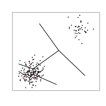
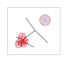
Figure 1: Left: A two-dimensional dataset. Middle: Voronoi tesselation from $k$-means clustering with $k=6$. Right: Our method converts the Voronoi tesselation into a union of (overlapping) six spheres. These spheres merge to form two clusters.

Paper Outline. We review $k$-means clustering in Section 2.1. We explain conformal prediction in Section 2.2. Our new approach, applied to $k$-means clustering, is described in Sections 3 and 3.2. Section 4 shows that we can use the same reasoning to convert mixture model clustering into a union of spheres. In Section 5 we introduce a new family of distributions called a max-mixture. This allows us to relate unions of spheres with level sets of densities. We show that level sets of certain functions can also be converted into unions of spheres clustering in Section 6.

2 Background

2.1 $k$-means Clustering

In this section, we briefly review $k$-means clustering, and we discuss some of its drawbacks. Let $Y_{1},\ldots,Y_{n}\sim P$ be iid draws from a distribution $P$ where $Y_{i}\in\mathbb{R}^{d}$. The $k$-means cluster centers $c_{1},\ldots,c_{k}\in\mathbb{R}^{d}$ are chosen to minimize

$$R(k)=\frac{1}{n}\sum_{i=1}^{n}\min_{j}||Y_{i}-c_{j}||^{2}.$$ (3)

The Voronoi cell $V_{j}$ is defined to be

$$V_{j}=\Bigl{\{}y:\ ||y-c_{j}||\leq||y-c_{s}||\ {\rm for\ all\ }s\neq j\Bigr{\}}.$$ (4)

Thus, $V_{j}$ consists of the points closest to $c_{j}$. The Voronoi cells $V_{1},\ldots,V_{k}$ define the clusters. In particular, the $j^{\rm th}$ data cluster is $C_{j}=\{Y_{i}:\ Y_{i}\in V_{j}\}$.

Despite its simplicity, $k$-means has many drawbacks:

1. Despite years of research, there is no agreed upon standard method for choosing $k$.

2. The Voronoi cells can be rather unnatural shapes that don’t reflect what we mean by a cluster.

3. If the clusters are roughly spherical and well separated, $k$-means works well. But in other cases, it can do poorly. One way to deal with this problem is to use a large value of $k$ and then merge some of the clusters. This gives a much more flexible clustering method. But it is not clear how to decide when to merge clusters.

4. In some sense, the ideal clusters with prediction coverages are the upper level sets of the density $p$ since the level sets are the minimum volume predictive sets with the natural clusters induced by connected components of them. [8, 4] One could try to estimate these using density estimation but this can be difficult in multivariate problems. It would be useful if $k$-means clustering could be used as an approximation to level set clustering. But no such results exist.

As we shall see, our predictive approach provides solutions, simultaneously, to all these problems. Before explaining the method, we need to discuss conformal prediction.

2.2 Conformal Prediction

Conformal prediction [9] is a general method for constructing distribution-free prediction sets. The basic idea is to test the hypothesis $H_{0}:Y=y$ that a future observation $Y$ takes the value $y$. The test is based on a set of residuals or conformal score. The test is performed for all values of $y$. By inverting the test, we get a prediction region. The precise steps are given in Algorithm 1.

Conformal Algorithm 1. Fix $Y_{n+1}=y$ where $y$ is an arbitrary value. Define the augmented dataset $${\cal A}(y)=\{Y_{1},\ldots,Y_{n},Y_{n+1}\}.$$ 2. For $i=1,\ldots,n+1$ let $R_{i}(y)=\phi(Y_{i},{\cal A})$ where $\phi$ is any function that is invariant to permutations of the elements of ${\cal A}$. $R_{i}(y)$ is called the conformal residual. 3. Let $$\pi(y)=\frac{1}{n+1}\sum_{i=1}^{n+1}I(R_{i}(y)\geq R_{n+1}(y)).$$ (5) 4. Repeat the above steps for every $y$ and set $$C_{n}=\Bigl{\{}y:\ \pi(y)\geq\alpha\Bigr{\}}=\Biggl{\{}y:\ \frac{1}{n+1}\sum_{i=1}^{n+1}I\Bigl{(}R_{i}(y)\geq R_{n+1}(y)\Bigr{)}\geq\alpha\Biggr{\}}.$$

List of Algorithms 1 The basic conformal algorithm.

The quantity $\pi(y)$ in (5) can be thought of as a p-value for testing the hypothesis $H_{0}:Y=y$. The residuals $R_{1},\ldots,R_{n+1}$ are exchangeable under $H_{0}$ so that $\pi(y)$ is uniformly distributed on $\{1/(n+1),\ldots,1\}$. The last step inverts the test to get a confidence set for $Y_{n+1}$. It follows that, for every distribution $P$,

$$P^{n+1}(Y\in C_{n})\geq 1-\alpha$$ (6)

where $Y$ is a new observation. For a proof of this fact see [9].

A simple example of a conformal residual is $R_{i}(y)=|Y_{i}-\overline{Y}_{y}|$ where $\overline{Y}_{y}=(Y_{1}+\cdots+Y_{n}+y)/(n+1)$ is the mean of the augmented data. The resulting prediction set is then

$$C_{n}=\Biggl{\{}y:\ \frac{1}{n+1}\sum_{i=1}^{n+1}I\Bigl{(}|Y_{i}-\overline{Y}(y)|\geq|y-\overline{Y}(y)|\Bigr{)}\geq\alpha\Biggr{\}}.$$

The choice of residual function $\phi$ does not affect the validity — that is the coverage — of $C_{n}$. But it does affect the size of $C_{n}$. In some sense, the optimal choice is $R_{i}=1/p(Y_{i})$; see [4]. As we explain in the next section, clustering can be used to construct the residuals which turns the clustering method into a prediction method. A similar idea was used in [5] for the purpose of clustering functional data.

Split Conformal Prediction. A modified algorithm called split conformal prediction is much faster than the standard conformal method. As the name implies, the method uses data splitting. Suppose the residuals have the form $R_{i}=\phi(Q,Y_{i})$ for some function $Q$ of the data. We use half the data to compute $Q$, and we compute the residuals on the other half of the data. We then get a prediction region by choosing the appropriate quantile of the residuals. The details are in Algorithm 2.

Split Conformal Algorithm 1. Split the data into two halves ${\cal Y}_{1}$ and ${\cal Y}_{2}$. 2. Compute $Q$ from ${\cal Y}_{1}$. 3. Compute the residuals $R_{i}=\phi(Q,Y_{i})$ where $Y_{i}\in{\cal Y}_{2}$. 4. Let $t_{\alpha}$ be the $1-\alpha$ quantile of the residuals. 5. Let $C_{n}=\{y:\ \phi(Q,y)\leq t_{\alpha}\}.$

List of Algorithms 2 The split conformal algorithm.

The set $C_{n}$ again has the distribution-free property

$$\inf_{P}P(Y_{n+1}\in C_{n})\geq 1-\alpha.$$

Split conformal inference is much faster than full conformal inference because it avoids the augmentation step.

3 From $k$-Mean Clustering to $k$-Spheres Clustering

We can combine prediction with $k$-means clustering by defining residuals from the clustering and then applying conformal prediction. As we shall see, the resulting prediction set can be used to define modified clusters. We will use split conformal prediction. So the first step is to split randomly the data into two groups ${\cal Y}_{1}$ and ${\cal Y}_{2}$. For simplicity, assume each group has a size of $n$.

3.1 The Basic Method

Let $c_{1},\ldots,c_{k}$ denote the cluster centers after applying $k$-means clustering to ${\cal Y}_{1}$. Define the residual

$$R_{i}=\min_{j}||Y_{i}-c_{j}||:=||Y_{i}-c_{j(i)}||$$

for each $Y_{i}\in{\cal Y}_{2}$. Here, $c_{j(i)}$ is the cluster center closest to $Y_{i}$. Now apply the conformal algorithm from the last section to get a conformal prediction set $C_{k}$. The precise steps are given in Algorithm 3.

Converting $k$-means to $k$-Spheres 1. Split the data into two halves ${\cal Y}_{1}$ and ${\cal Y}_{2}$. 2. Run $k$-means on ${\cal Y}_{1}$ to get centers $c_{1},\ldots,c_{k}$. 3. For the data in ${\cal Y}_{2}$ compute the (non-augmented) residuals $$R_{i}=||Y_{i}-c_{j(i)}||$$ where $c_{j(i)}$ is the closest center to $Y_{i}$. 4. Let $t_{\alpha}$ be the $1-\alpha$ quantile of the residuals. 5. Let ${\cal C}_{k}=\{y:\ \min_{j}||y-c_{j}||\leq t_{\alpha}\}$. 6. Choose $\widehat{k}$ to minimize $\mu({\cal C}_{k})$ where $\mu$ is Lebesgue measure. 7. Return: ${\cal C}_{\widehat{k}}$.

List of Algorithms 3 This algorithm converts $k$-means clustering into $k$-spheres clustering.

From the definition of the residuals, together with the definition of ${\cal C}_{k}$ we immediately see that ${\cal C}_{k}$ is a union of spheres. We this have:

Lemma 1.

The conformal set has the form

$${\cal C}_{k}=\bigcup_{j=1}^{k}B(c_{j},t_{\alpha})$$ (7)

where $t_{\alpha}$ is defined in Step 4 of Algorithm 3. If $Y$ denotes a new observation, then

$$\inf_{P}P^{n+1}(Y\in{\cal C}_{k})\geq 1-\alpha$$ (8)

where the infimum is over all distributions $P$.

Every choice of $k$ gives a valid prediction set ${\cal C}_{k}$ with the correct coverage. We choose $k$ to minimize the Lebesgue measure of ${\cal C}_{k}$. Unlike the within sums of squares — which strictly decreases with $k$ — the Lebesgue measure typically decreases then, eventually increases as $k$ increases. Thus we define

$$\widehat{k}=\operatorname*{argmin}_{k}\mu({\cal C}_{k}).$$ (9)

The final clustering is ${\cal C}_{\widehat{k}}$. We have now replaced the Voronoi tesselation with more intuitively shaped sets. Also, some of the spheres may be connected (overlapping). In other words, we have automatically merged the clusters.

Remark 1: To check whether spheres are connected to each other, we examine whether there exists at least a single point in intersections of spheres. This sample-based connectivity checking rule might possibly fail to find some weak connections among spheres. In practice, however, we can obtain stable clusters by using the sample-based rule to disconnect weakly connected spheres.

Remark 2: To preserve the prediction guarantee, we can restrict $k$ to be in some large range $1\leq k\leq K_{n}$ and replace $\alpha$ with $\alpha/K_{n}$. Here, $K_{n}$ can increase with $n$. The union bound then ensures that the coverage guarantee is still valid even after selecting $k$. However, as we view clustering mainly as an exploratory tool, it is not crucial to do this correction.

The Lebesgue measure $\mu(C_{k})$ can be easily estimated using importance sampling. For example, we can draw $Z_{1},\ldots,Z_{N}$ from any convenient density $g$ (such as a uniform density over a large region) and then we have that

$$\mu(C_{k})=\int_{C_{k}}d\mu=\int_{C_{k}}\frac{g(u)}{g(u)}d\mu(u)\approx\frac{1}{N}\sum_{j=1}^{N}\frac{I(Z_{j}\in C_{k})}{g(Z_{j})}.$$

The residual $R_{i}=||Y_{i}-c_{j(i)}||$ is simple and intuitive. But, due to the generality of conformal prediction, we have the liberty of choosing any permutation invariant residual. In fact, much better clusters can be obtained by defining

$$R_{i}=\min_{j\in[k]}\left[\frac{||Y_{i}-c_{j}||^{2}}{\widehat{\sigma}_{j}^{2}}+2d\log\widehat{\sigma}_{j}-2\log\widehat{\pi}_{j}\right]$$ (10)

where $\widehat{\pi}_{n}=n_{j}/n$, $n_{j}$ is the number of points from ${\cal Y}_{1}$ in $V_{j}$, and

$$\widehat{\sigma}_{j}^{2}=n_{j}^{-1}\sum_{Y_{i}\in C_{j}}||Y_{i}-\overline{Y}_{j}||^{2}.$$

Let $t_{\alpha}$ be the $1-\alpha$ quantile of the residuals. Now we use Algorithm 3 but with the residuals defined as in (10). Denote the resulting conformal prediction region by ${\cal M}_{k}$. From the definition of $M_{k}$ together with the basic property of the conformal prediction we have:

Lemma 2.

We have that

$${\cal M}_{k}=\bigcup_{j=1}^{k}B(c_{j},r_{j})$$

where

$$r_{j}=\widehat{\sigma}_{j}\sqrt{[t_{\alpha}+2\log\widehat{\pi}_{j}-2d\log\widehat{\sigma}_{j}]_{+}}.$$

Furthermore, $\inf_{P}P^{n+1}(Y\in{\cal M}_{k})\geq 1-\alpha$.

As before we choose $k$ to minimize $\mu({\cal M}_{k})$.

Example 3.

Figure 2 illustrate how the algorithm for converting $k$-means clustering into $k$-spheres clustering works. The left panel shows the data generated from four Normal distributions with background noise. The middle panel shows how the volume of clusters changes as $k$ varying from $1$ to $20$. The right panel shows clusters with the minimum volume ($k=4$). The resulting clusters are $1-\alpha$ predictive region with $\alpha=0.1$.

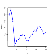
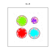
Figure 2: Left: A two-dimensional dataset. Middle: $k$ versus volume of clusters. Right: Clusters with the minimum volume.

Note that if we chose $k$ to minimize the usual within sums-of-squares, then we always end up choosing $k=n$. This is why choosing $k$ is so hard in $k$-means clustering. Fortunately, this does not happen in our approach. In fact, if the data points are well-separated into $k^{*}<n$ spherical clusters, then $\mu(M_{k})$ is minimized at $k=k^{*}<n$. We see this in Figure 3, which shows what happens when we let $k$ grow.

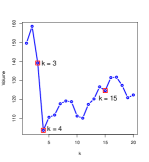
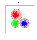
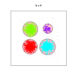
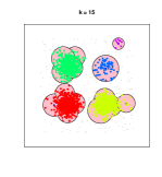
Figure 3: From left to right : Volumes of clusters and clusters with $k=3,4,15$.

3.2 Improving the Choice of $k$ With Hypothesis Testing

So far we have chosen $\widehat{k}$ to minimize $S_{k}\equiv\mu(C_{k})$. Now, $S_{k}$ is a random variable and we can end up choosing a large $k$ due to random fluctuations. The resulting clustering, even in such cases, can be quite reasonable. Still, it is sometimes useful to use simpler clusterings with small $k$ when possible. To this end, we can use a hypothesis testing approach to choose $k$.

Let $\nu_{k}=\mathbb{E}[S_{k}]$ be the mean of $S_{k}$. For $k=K,K-1,\ldots,1$ we will test the hypothesis

$$H_{0}^{k}:\nu_{t}<\nu_{k}\ \ {\rm for\ some\ t<k}.\ \ \ \ \ {\rm versus}\ \ \ \ \ H_{1}^{k}:\nu_{k}\leq\nu_{t}\ \ {\rm for\ all\ t<k}.$$

We choose $\widehat{k}$ to be the first $k$ for which this hypothesis is rejected. We will construct a confidence interval $A_{t,k}$ for the parameter

$$\theta_{t,k}=\nu_{t}-\nu_{k}.$$ (11)

For each $k$, if every value in $\bigcup_{t<k}A_{t,k}$ is positive, we reject $H_{0}^{k}$. To construct $A_{t,k}$ we use the bootstrap. For each pair of $t<k$, we approximate the cdf

$$F_{n}^{k}(t)=P(\sqrt{n}|S_{t}-S_{k}-\theta_{t,k}|\leq t)$$

with its bootstrap approximation

$$\widehat{F}_{n}^{k}(t)=\frac{1}{B}\sum_{j=1}^{B}I(\sqrt{n}|S_{t}^{(j)}-S_{k}^{(j)}-(S_{t}-S_{k})|\leq t)$$

where $S^{(1)},\ldots,S^{(B)}$ denote bootstrap replications. Let

$$z_{1-{\alpha/2}}=\widehat{F}_{n}^{-1}(1-\alpha/2)$$

$$z_{\alpha/2}=\widehat{F}_{n}^{-1}(\alpha/2)$$

and let

$$A_{t,k}=\left\{\theta:2(S_{t}-S_{k})-z_{1-\alpha/2/(k-1)}<\theta<2(S_{t}-S_{k})-z_{\alpha/2/(k-1)}\right\},~{}~{}\forall t=1,\dots,k-1$$

Then, $A_{1,k},\dots,A_{k-1,k}$ are asymptotic $1-\alpha$ confidence sets for $\theta_{1,k},\dots,\theta_{t,k}$. We reject $H_{0}$ if $\min\{a\in\bigcup_{t<k}A_{t,k}\}>0$.

4 Mixture Models

The same approach can be used with mixture models. Let

$$p_{k}(y)=\sum_{j=1}^{k}\pi_{j}\phi(y;\mu_{j},\Sigma_{j})$$

denote a mixture of Gaussians where $\phi(x;\mu_{j},\Sigma_{j})$ denotes a Normal density with mean vector $\mu_{j}$ and covariance matrix $\Sigma_{j}$. In this case, we define the residual to be

$$R_{i}=\min_{j\in[k]}\left[\frac{1}{\widehat{\pi}_{j}\phi(Y_{i};\widehat{\mu}_{j},\widehat{\Sigma}_{j})}\right]$$ (12)

or

$$R_{i}=\min_{j}\left[\frac{1}{2}(Y_{i}-\mu_{j})^{T}\Sigma_{j}^{-1}(Y_{i}-\mu_{j})+\frac{1}{2}\log\det(\Sigma_{j})-\log\pi_{j}\right].$$ (13)

We note that a similar residual was used in [5] in the context of functional clustering. The resulting conformal prediction set is a union of ellipses:

$${\cal C}_{k}=\bigcup_{j=1}^{k}E(\widehat{\mu}_{j},\widehat{\Sigma}_{j},r_{j})$$ (14)

where $t_{\alpha}$ is the $1-\alpha$ quantile of the residuals, $E(a,A,b)=\{y:\ (y-a)^{T}A^{-1}(y-a)\leq b^{2}\}$ and

$$r_{j}^{2}=\left[\log\widehat{\pi}_{j}+\log t_{\alpha}-\frac{d}{2}\log(2\pi)-\frac{1}{2}\log|\widehat{\Sigma}_{j}|\right]_{+}.$$

The clusters are the connected components of ${\cal C}_{k}$. Again, we see that the method automatically merges components that are near each other and $k$ can be chosen to minimizing the volume of ${\cal C}_{k}$.

Note that our residual is precisely the residual in (10) except that $k$-means replaces maximum likelihood and Euclidean distance replaces Mahalanobis distance. Thus the method based on (10) can be thought of as an approximate approach to conformalized mixtures of Gaussians. This connection can be made more formal, as we show in the next section.

Example 4.

Figure 4 illustrates how the algorithm for converting mixture models into $k$-ellipsoids clustering works. The left panel shows the data generated from three Normal distributions with different covariance structures in addition to background noises. The middle panel shows how the volume of clusters changes as $k$ varying from $1$ to $10$. The shaded lines corresponds to volume curves with bootstrapped data. The right panel shows clusters with $k=4$ which is selected by the testing based method in the previous section. Note that there are only three ellipsoids even if the clustering is based on mixture of four Normal distributions since $r_{j}=0$ for one of ellipsoidal clusters (blue dot in the middle). The resulting clusters are $1-\alpha$ predictive region with $\alpha=0.1$.

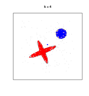
Figure 4: Left: A two-dimensional dataset. Middle: $k$ versus volume of clusters. Right: Clusters with minimum volume.

5 A Max-Mixture Model

In this section we link unions of spheres — and more generally, unions of ellipsoids — to level sets of densities by introducing a modified mixture model.

Let $\theta=\{\pi_{j},\mu_{j},\Sigma_{j}\}_{j=1}^{k}$ and define the density

$$p(y;\theta)=\frac{\max_{1\leq j\leq k}\pi_{j}\phi(y;\mu_{j},\Sigma_{j})}{Z_{\theta}}$$ (15)

where $Z_{\theta}=\int\max_{1\leq j\leq k}\pi_{j}\phi(y;\mu_{j},\Sigma_{j})$. Let ${\cal F}_{k}$ be all such densities. We call this the max-mixture model.

The $1-\alpha$ upper level set of $f(y;\theta)\in\mathcal{F}_{k}$ is the union of ellipsoids of the following form:

$$\widetilde{C}^{(\alpha)} :=\{y:f(y;\theta)\geq t^{(\alpha)}\}$$

$$=\bigcup_{j=1}^{k}\left\{y:(y-\mu_{j})^{T}\Sigma_{j}^{-1}(y-\mu_{j})\leq-2\log\det(\Sigma_{j})+2\log\pi_{j}+M^{(\alpha)}\right\}$$

where $t^{(\alpha)},M^{(\alpha)}\in\mathbb{R}$ are constants chosen to make $P(\widetilde{C}^{(\alpha)})\geq 1-\alpha$. Hence, for this modified mixture family, upper level sets correspond exactly with unions of ellipsoids. Of course, we strict $\Sigma_{j}$ to be of the form $\sigma_{j}^{2}I$ then we get a union of spheres.

The negative log-likelihood for this model is

$$\ell(\theta):= \frac{1}{n}\sum_{i=1}^{n}\min_{j}\left[\frac{1}{2}(Y_{i}-\mu_{j})^{T}\Sigma_{j}^{-1}(Y_{i}-\mu_{j})+\frac{1}{2}\log\det(\Sigma_{j})-\log\pi_{j}\right]$$ (16)

$$+\log\int\max_{j\in[k]}\pi_{j}\phi(y;\mu_{j},\Sigma_{j})(y)\mathrm{d}y.$$

Minimizing $\ell(\theta)$ is difficult because of the integral. Solutions of (Generalized) k-means and maximum likelihood of Gaussian mixture problems can be interpreted as two approximate minimizers of $\ell(\theta)$.

5.1 (Generalized) k-means : Minimize the first term of $\ell(\theta)$

We can obtain an approximate minimizer by using the first part of $\ell(\theta)$ as the objective function. That is, we estimate the parameters by minimizing

$$\ell_{kM}(\theta):=\frac{1}{n}\sum_{i=1}^{n}\min_{j}\left[\frac{1}{2}(Y_{i}-\mu_{j})^{T}\Sigma_{j}^{-1}(Y_{i}-\mu_{j})+\frac{1}{2}\log\det(\Sigma_{j})-\log\pi_{j}\right].$$ (17)

Proposition 5.

For any $\theta=\{\pi_{j},\mu_{j},\Sigma_{j}\}_{j=1}^{k}$, we have the following bound :

$$\ell_{kM}(\theta)-\log k\leq\ell(\theta)\leq\ell_{kM}(\theta).$$ (18)

Therefore, for any $\theta^{\dagger}$ and $\theta^{*}$ minimizing $\ell$ and $\ell_{kM}$ we get

$$\left|\ell(\theta^{\dagger})-\ell(\theta^{*})\right| \leq\log k,\ \ \ {\rm and}\ \ \ \left|\ell_{kM}(\theta^{\dagger})-\ell_{kM}(\theta^{*})\right|\leq\log k.$$

Proof.

It is enough to show that

$$-\log k\leq\log\int\max_{j\in[k]}\pi_{j}\phi(y;\mu_{j},\Sigma_{j})(y)\mathrm{d}y\leq 0$$

Since each $\phi(y;\mu_{j},\Sigma_{j})(y)$ is a density function, the first inequality is followed by

$$-\log k =\log\left(\frac{1}{k}\sum_{j=1}^{k}\pi_{j}\right)=\log\left(\frac{1}{k}\sum_{j=1}^{k}\pi_{j}\int\phi(y;\mu_{j},\Sigma_{j})(y)\mathrm{d}y\right)$$

$$=\log\int\frac{1}{k}\sum_{j=1}^{k}\pi_{j}\phi(y;\mu_{j},\Sigma_{j})(y)\mathrm{d}y\leq\log\int\max_{j\in[k]}\pi_{j}\phi(y;\mu_{j},\Sigma_{j})(y)\mathrm{d}y.$$

The second inequality is follows since

$$\log\int\max_{j\in[k]}\pi_{j}\phi(y;\mu_{j},\Sigma_{j})(y)\mathrm{d}y \leq\log\int\sum_{j=1}^{k}\pi_{j}\phi(y;\mu_{j},\Sigma_{j})(y)\mathrm{d}y$$

$$=\log\sum_{j=1}^{k}\pi_{j}\int\phi(y;\mu_{j},\Sigma_{j})(y)\mathrm{d}y=\log\sum_{j=1}^{k}\pi_{j}=0.$$

∎

If we restrict to $\Sigma_{j}\in\{\sigma^{2}\mathrm{I}:\sigma\in\mathbb{R}\}$ and set $\pi_{j}=\frac{1}{k}$ for all $j=1,\dots,k$, then minimizing $\ell$ is the same as the ordinary $k$-means problem. Generally, Lloyd’s algorithm can be directly extended to find a local optimum of the generalized $k$-means problem. The details are in Algorithm 4.

Generalized Lloyd’s Algorithm 1. Initialize $\theta_{j}=(\pi_{j},\mu_{j},\Sigma_{j})$ for $j=1,\dots,k$. 2. Set $$w_{i,j}=\left\{\begin{array}[]{ll}1&\text{if~{}~{}}j=\operatorname*{argmin}_{l}\frac{1}{2}(Y_{i}-\mu_{l})^{T}\Sigma_{l}^{-1}(Y_{i}-\mu_{l})+\frac{1}{2}\log\det(\Sigma_{l})-\log\pi_{l}\\ 0&\text{otherwise}\end{array}\right.$$ 3. Update $\mu_{j}^{+}=\frac{1}{\sum_{i=1}^{n}w_{i,j}}\sum_{i=1}^{n}w_{i,j}Y_{i}$, for all $j=1,\dots,k$. 4. Update $\Sigma_{j}^{+}=\frac{1}{\sum_{i=1}^{n}w_{i,j}}\sum_{i=1}^{n}w_{i,j}(Y_{i}-\mu_{j}^{+})(Y_{i}-\mu_{j}^{+})^{T}$ , for all $j=1,\dots,k$. 5. Update $\pi_{j}^{+}=\frac{1}{n}\sum_{i=1}^{n}w_{i,j}$, for all $j=1,\dots,k$. 6. Repeat step 2-5 until converge.

List of Algorithms 4 The generalized version of Lloyd’s algorithm for the Max-Mixture Model.

5.2 Gaussian Mixture: Minimize another upper and lower bounds of $\ell(\theta)$

The negative log-likelihood of Gaussian mixture model can be rewritten as

$$\ell_{GM}(\theta):=-\frac{1}{n}\sum_{i=1}^{n}\log\left[\sum_{j=1}^{k}\exp\left\{-\frac{1}{2}(Y_{i}-\mu_{j})^{T}\Sigma_{j}^{-1}(Y_{i}-\mu_{j})-\frac{1}{2}\log\det(\Sigma_{j})+\log\pi_{j}\right\}\right].$$

Proposition 6.

For any $\theta=\{\pi_{j},\mu_{j},\Sigma_{j}\}_{j=1}^{k}$, we have the following bound :

$$\ell_{GM}(\theta)-\log k\leq\ell(\theta)\leq\ell_{GM}(\theta)+\log k.$$ (19)

Therefore, for any $\theta^{\dagger}$ and $\theta^{*}$ minimizing $\ell$ and $\ell_{GM}$ we get

$$\left|\ell(\theta^{\dagger})-\ell(\theta^{*})\right| \leq 2\log k,\ \ \ {\rm and}\ \ \ \left|\ell_{GM}(\theta^{\dagger})-\ell_{GM}(\theta^{*})\right|\leq 2\log k.$$

Proof.

From Proposition 5, we know that

$$\ell_{kM}(\theta)-\log k\leq\ell(\theta)\leq\ell_{kM}(\theta).$$

Therefore, it is enough to show that

$$\ell_{GM}(\theta)\leq\ell_{kM}(\theta)\leq\ell_{GM}(\theta)+\log k$$

Note that

$$\ell_{kM}(\theta) =\frac{1}{n}\sum_{i=1}^{n}\min_{j}\left[\frac{1}{2}(Y_{i}-\mu_{j})^{T}\Sigma_{j}^{-1}(Y_{i}-\mu_{j})+\frac{1}{2}\log\det(\Sigma_{j})-\log\pi_{j}\right]$$

$$=\frac{1}{n}\sum_{i=1}^{n}\log\left[\exp\left\{\min_{j\in[k]}\frac{1}{2}(Y_{i}-\mu_{j})^{T}\Sigma_{j}^{-1}(Y_{i}-\mu_{j})+\frac{1}{2}\log\det(\Sigma_{j})-\log\pi_{j}\right\}\right]$$

$$=-\frac{1}{n}\sum_{i=1}^{n}\log\left[\max_{j\in[k]}\exp\left\{-\frac{1}{2}(Y_{i}-\mu_{j})^{T}\Sigma_{j}^{-1}(Y_{i}-\mu_{j})-\frac{1}{2}\log\det(\Sigma_{j})+\log\pi_{j}\right\}\right]$$

Hence, the first inequality comes from

$$\ell_{kM}(\theta) =-\frac{1}{n}\sum_{i=1}^{n}\log\left[\max_{j\in[k]}\exp\left\{-\frac{1}{2}(Y_{i}-\mu_{j})^{T}\Sigma_{j}^{-1}(Y_{i}-\mu_{j})-\frac{1}{2}\log\det(\Sigma_{j})+\log\pi_{j}\right\}\right]$$

$$\geq-\frac{1}{n}\sum_{i=1}^{n}\log\left[\sum_{j=1}^{k}\exp\left\{-\frac{1}{2}(Y_{i}-\mu_{j})^{T}\Sigma_{j}^{-1}(Y_{i}-\mu_{j})-\frac{1}{2}\log\det(\Sigma_{j})+\log\pi_{j}\right\}\right]$$

$$=\ell_{GM}(\theta)$$

And the second inequality is followed by

$$\ell_{kM}(\theta) =-\frac{1}{n}\sum_{i=1}^{n}\log\left[\max_{j\in[k]}\exp\left\{-\frac{1}{2}(Y_{i}-\mu_{j})^{T}\Sigma_{j}^{-1}(Y_{i}-\mu_{j})-\frac{1}{2}\log\det(\Sigma_{j})+\log\pi_{j}\right\}\right]$$

$$\leq-\frac{1}{n}\sum_{i=1}^{n}\log\left[\frac{1}{k}\sum_{j=1}^{k}\exp\left\{-\frac{1}{2}(Y_{i}-\mu_{j})^{T}\Sigma_{j}^{-1}(Y_{i}-\mu_{j})-\frac{1}{2}\log\det(\Sigma_{j})+\log\pi_{j}\right\}\right]$$

$$=\ell_{GM}(\theta)+\log k$$

∎

The standard EM algorithm can be used to get a local minimum of $\ell_{GM}(\theta)$.

5.3 Union of ellipsoids clustering - General algorithm.

To get $1-\alpha$ upper level set of $p(y;\theta)$, we can directly use the split conformal prediction method with the residual function $-p(y;\theta)$. However, to evaluate $-p(y;\theta)$, we need to calculate the normalizing constant$\int\max_{j\in[k]}\pi_{j}\phi(y;\mu_{j},\Sigma_{j})(y)$. Since the constant does not depend on $y$, we use an equivalent residual function defined by

$$\widetilde{p}(y;\theta)=\min_{j\in[k]}\left[(y-\mu_{j})^{T}\Sigma_{j}^{-1}(y-\mu_{j})+\log\det(\Sigma_{j})-2\log\pi_{j}\right].$$ (20)

This is equivalent to residual functions defined in (10) and (12) except how we estimate the parameters. The general split conformal steps are in Algorithm 5.

Unions of Ellipses 1. Split the data into two halves ${\cal Y}_{1}$ and ${\cal Y}_{2}$. 2. Estimate $\widehat{\theta}$ from ${\cal Y}_{1}$ by solving generalized k-means or maximum likelihood problem of GMM. 3. Compute the residuals $$R_{i}=\widetilde{f}(Y_{i};\widehat{\theta})=\min_{j\in[k]}\left[(Y_{i}-\widehat{\mu}_{j})^{T}\widehat{\Sigma}_{j}^{-1}(Y_{i}-\widehat{\mu}_{j})+\log\det(\widehat{\Sigma}_{j})-2\log\widehat{\pi}_{j}\right]$$ where $Y_{i}\in{\cal Y}_{2}$. 4. Let $M^{(\alpha)}$ be the $1-\alpha$ quantile of the residuals. 5. Let $\displaystyle\widetilde{C}^{(\alpha)}$ $\displaystyle=\{y:\widetilde{f}(y;\widehat{\theta})\leq M^{(\alpha)}\}$ (21) $\displaystyle=\bigcup_{j=1}^{k}\left\{y:(y-\mu_{j})^{T}\Sigma_{j}^{-1}(y-\mu_{j})\leq-2\log\det(\Sigma_{j})+2\log\pi_{j}+M^{(\alpha)}\right\}.$ (22)

List of Algorithms 5 Obtaining a union of ellipses from the generalized Lloyd’s algorithm.

We now see that $\widetilde{C}^{(\alpha)}$ is a union of ellipsoids with $1-\alpha$ coverage, that is,

$$\mathbb{P}(Y_{n+1}\in\widetilde{C}^{(\alpha)})=P(\widetilde{C}^{(\alpha)})\geq 1-\alpha$$

Unlike common mixture model based clustering, our method defines clusters as connected components of a level set which make it possible to apply our method to general shaped clusters.

Figure 5 shows an example. Panel (a) shows the data with 4 crescent-shaped clusters. Panel (b - d) show the resulting clusters in which parameter estimations are based on $k$-means, generalized $k$-means, and a Gaussian mixture model, respectively. Each union of balls/ellipsoids is a $1-\alpha$ predictive region of the underlying distribution with $\alpha=0.1$. Although some of the methods yield small erroneous clusters, all method recover the crescent-shaped areas reasonably.

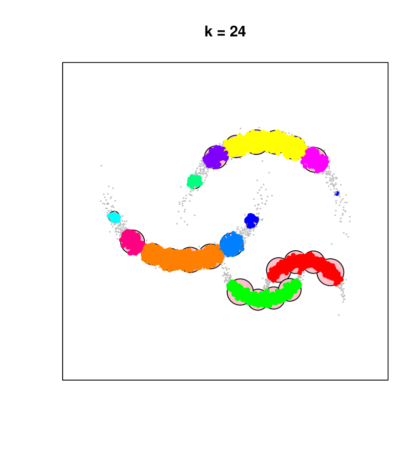
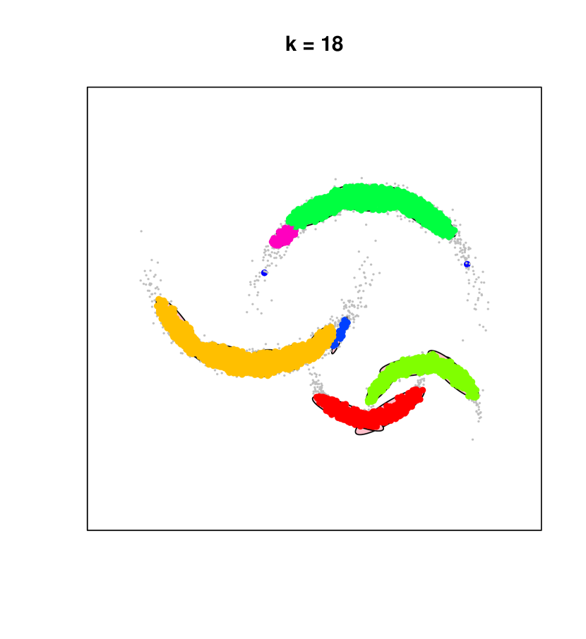
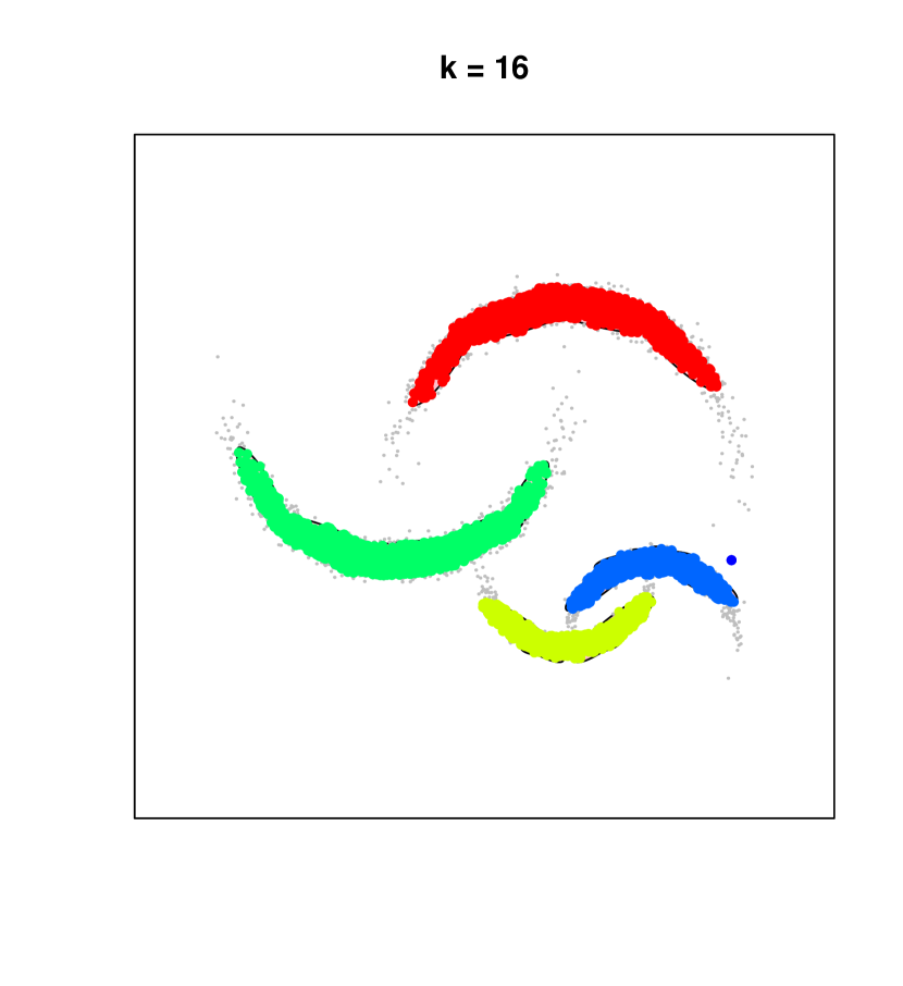
Figure 5: (a) A two-dimensional dataset. (b) k-means. (c) Generalized k-means. (d) GMM.

6 Converting Level Sets to Unions of Spheres

Another approach to clustering is to use the upper level sets of density estimates. These can easily be converted into unions of spheres. We focus on $k$-nearest neighbor density estimation.

6.1 Density Functions

Let $L=\{y:\ \widehat{p}(y)>t\}$ be the upper level set of a nonparametric density estimator $\widehat{p}$. The set $L$ is often used for clustering; see [2], for example. In general, $L$ is a very complex set and is hard to compute. In general, there is no simple way to represent this set. Some authors have suggested approximating $L$ with a union of spheres. In this section, we show that the conformalization approach automatically turns $L$ into a union of spheres and that, as with the other approaches, minimizing volume allows us to choose all tuning parameters. The details are in Algorithm 6.

Density Level Set Conversion 1. Split the data into two halves ${\cal Y}_{1}$ and ${\cal Y}_{2}$. 2. Estimate a density $\widehat{p}$ from ${\cal Y}_{1}$. 3. For a given $t>0$, let ${\cal Y}_{1}^{(t)}:=\{Y_{i}\in{\cal Y}_{1}:\widehat{p}(Y_{i})\geq t\}$. 4. Compute the residuals $R_{i}:=R(Y_{i})$ for $Y_{i}\in{\cal Y}_{2}$, where $R(y)=\min_{Y_{j}\in{\cal Y}_{1}^{(t)}}\|y-Y_{j}\|$. 5. Let $M^{(\alpha)}$ be the $1-\alpha$ quantile of the residuals. 6. Let $\widehat{C}^{(\alpha)}=\{y:R(y)\leq M^{(\alpha)}\}=\bigcup_{Y_{j}\in{\cal Y}_{1}^{(t)}}\left\{y:\|y-Y_{j}\|\leq M^{(\alpha)}.\right\}$

List of Algorithms 6 Algorithm to convert density level set into a union of spheres.

Recall that the $k$-nn density estimate is $\widehat{p}(x)=k/(nd_{k}(x))$ where $d_{k}(x)$ is the distance from $x$ to its $k^{\rm th}$ nearest-neighbor. The resulting set $\widehat{C}^{(\alpha)}$ is a union of balls with $1-\alpha$ coverage, that is,

$$P^{n+1}(Y_{n+1}\in\widehat{C}^{(\alpha)})=P(\widehat{C}^{(\alpha)})\geq 1-\alpha.$$

We can minimize the Lebesgue measure to choose both tuning parameters $t$ and $k$.

Example 7.

Figure 6 illustrates the results of Algorithm 6. We use the same data with the crescent-shaped clusters as in the previous example. Panel (a) shows how the volume of the clusters changes as the parameter $k$ varying from $2^{1}$ to $2^{8}$ with the level $t$ fixed to the $1-\alpha$ quantile of density values from the first half data $\mathcal{Y}_{1}$. The shaded lines corresponds to volume curves with bootstrapped data. Panel (b) shows clusters with $k=32$ which is selected by the testing based method. Panel (c) illustrates how the volume of the clusters changes as the level parameter $t$ varying from $1-\alpha/2$ to $1-2\alpha$ quantiles of the density values of the first half data $\mathcal{Y}_{1}$ with fixed $k=32$. The shaded lines corresponds to volume curves with bootstrapped data. Panel (d) shows clusters with $k=32$, $t$ equal to the $1-0.112$ quantile of density values on the first half data $\mathcal{Y}_{1}$.

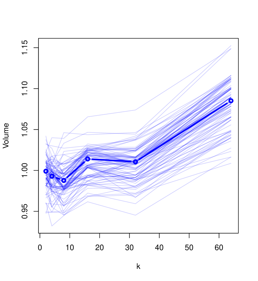
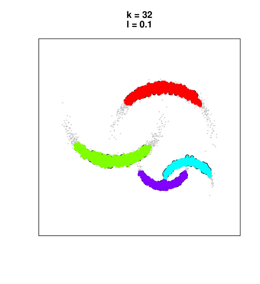
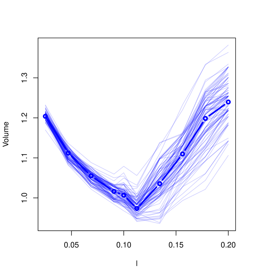
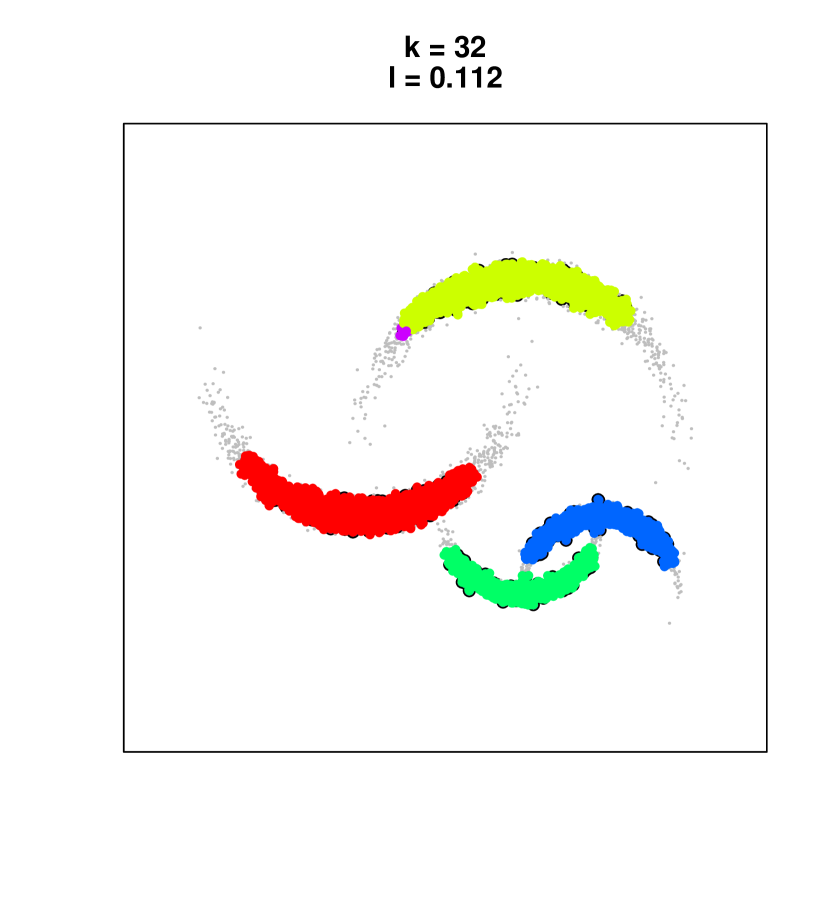
Figure 6: (a) $k$ versus volume curve with fixed level $t>0$. (b) k-NN level set clusters with $\widehat{k}$. (c) $t$ versus volume curve with fixed parameter $k=\widehat{k}$. (d) k-NN level set clusters with $\widehat{k}$ and $\widehat{t}.$

Remark: As with $k$-means we may want to use spheres of varying size. We can do this by introducing an adaptive residual function such as $R(y)=\min_{Y_{j}\in{\cal Y}_{1}^{(t)}}\|y-Y_{j}\|\sqrt{\widehat{p}(Y_{j})}$ for example. Then,

$$\widehat{C}^{(\alpha)}=\{y:R(y)\leq M^{(\alpha)}\}=\bigcup_{Y_{j}\in{\cal Y}_{1}^{(t)}}\left\{y:\|y-Y_{j}\|\leq\frac{M^{(\alpha)}}{\sqrt{\widehat{p}(Y_{j})}}\right\}.$$

7 Conclusion and Future Work

In this paper we showed that we can construct distribution-free prediction sets from clustering. These prediction sets can be regarded as an improved clustering. We can choose the tuning parameters in the clustering to minimize the volume of the prediction set.

There are some natural extensions of this approach. First, it would be interesting to create a streaming version of the method. In fact, the conformal prediction was originally presented as a sequential method. It may be possible, therefore, to incorporate streaming clustering as well. Second, there have been some papers on clustering in the regression framework [6, 1]. In these models, we let the clustering structure of $Y$ vary with $x$. We could adapt our methods to produce cluster-structured prediction sets. Such sets can be much smaller than standard regression prediction sets if there is a clustering structure in the data.

References

- Chen [2018] Yen-Chi Chen. Modal regression using kernel density estimation: A review. Wiley Interdisciplinary Reviews: Computational Statistics, 10(4):e1431, 2018.
- Cuevas et al. [2001] Antonio Cuevas, Manuel Febrero, and Ricardo Fraiman. Cluster analysis: a further approach based on density estimation. Computational Statistics & Data Analysis, 36(4):441–459, 2001.
- Kumar and Orlin [2008] Mahesh Kumar and James B Orlin. Scale-invariant clustering with minimum volume ellipsoids. Computers & Operations Research, 35(4):1017–1029, 2008.
- Lei et al. [2013] Jing Lei, James Robins, and Larry Wasserman. Distribution-free prediction sets. Journal of the American Statistical Association, 108(501):278–287, 2013.
- Lei et al. [2015] Jing Lei, Alessandro Rinaldo, and Larry Wasserman. A conformal prediction approach to explore functional data. Annals of Mathematics and Artificial Intelligence, 74(1-2):29–43, 2015.
- Loubes et al. [2017] Jean-Michel Loubes, Bruno Pelletier, et al. Prediction by quantization of a conditional distribution. Electronic journal of statistics, 11(1):2679–2706, 2017.
- Polonik et al. [1995] Wolfgang Polonik et al. Measuring mass concentrations and estimating density contour clusters-an excess mass approach. The Annals of Statistics, 23(3):855–881, 1995.
- Rinaldo et al. [2010] Alessandro Rinaldo, Larry Wasserman, et al. Generalized density clustering. The Annals of Statistics, 38(5):2678–2722, 2010.
- Shafer et al. [2005] G Shafer, A Gammerman, and V Vovk. Algorithmic Learning in a Random World. Springer, 2005.