Particle-Set Identification method to study multiplicity fluctuations

Abstract

In this paper a new method of experimental data analysis, the Particle-Set Identification method, is presented. The method allows to reconstruct moments of multiplicity distribution of identified particles. The difficulty the method copes with is due to incomplete particle identification – a particle mass is frequently determined with a resolution which does not allow for a unique determination of the particle type. Within this method the moments of order $k$ are calculated from mean multiplicities of $k$-particle sets of a given type. The Particle-Set Identification method remains valid even in the case of correlations between mass measurements for different particles. This distinguishes it from the Identity method introduced by us previously to solve the problem of incomplete particle identification in studies of particle fluctuations.

I Introduction

Study of multiplicity fluctuations of identified particles produced in high energy nucleus-nucleus collisions is motivated by a number of important physics issues. They include searching for the critical point of strongly interacting matter, uncovering properties of hadronization and testing the validity of statistical models beyond mean multiplicities of identified hadrons, see Refs. Koch:2008ia ; Gazdzicki:2015ska for details. Experimental measurements of multiplicity distributions of identified hadrons are challenging because it is often impossible to identify a particle with sufficient precision. Typical tracking detectors, like time projection chambers or silicon pixel detectors, used in high energy physics, allow for a precise measurement of momenta of charged particles and sign of their electric charges. In order to be able to distinguish between different particle types (e.g. e⁺, $\pi^{+}$, $K^{+}$, proton) a determination of particle mass is necessary. This is done indirectly by measuring for each particle the value of a special variable, e.g., specific energy loss, ${\textrm{d}}E\!/\!{\textrm{d}}x$, time-of-flight or the Cerenkov radiation angle. In the following this variable is referred to as the ”mass” variable. In 2011 the Identity method Gazdzicki:2011xz was proposed as a tool to measure moments of multiplicity distribution of identified particles, which circumvents the experimental issue of incomplete particle identification. The method was significantly developed in Ref. Gorenstein:2011hr and extended in following papers, see Refs. Rustamov:2012bx ; Pruneau:2017fim ; Pruneau:2018glv ; Mackowiak-Pawlowska:2017dma . Currently, the Identity method is used by several experimental collaborations Anticic:2013htn ; Mackowiak-Pawlowska:2013caa ; Acharya:2017cpf ; Rustamov:2017lio .

In this paper we present a novel approach, the Particle-Set (PSET) Identification method, for reconstructing moments of multiplicity distribution of identified particles. Hereinafter a PSET represents a set of $k$-particles ($k=2,3,\ldots$) which is constructed from particles created in a collision. For example, in the simplest non-trivial case of two particle types, pions and kaons, three types of two-particle sets are possible: pion-pion, kaon-kaon and pion-kaon. Mean multiplicities of different two-particle sets permit to calculate the second order moments of the joint multiplicity distribution of pions and kaons. To find the third order (in general, $k^{th}$ order) moments of the multiplicity distribution one needs mean multiplicities of three-particle (in general, $k$-particle) sets. The latter are obtained from fits to the $k$-dimensional distribution of particle masses. The PSET Identification method has a broader range of applicability than the Identity method. Particularly, it does not assume that measurements of masses for different particles are independent.

The paper is organized as follows. Section II introduces the PSET Identification method. For simplicity, the presentation in this section is restricted to second moments of the multiplicity distribution of two particle types, pions and kaons. First, the problem is defined and the well-known method to calculate mean multiplicities of identified hadrons is reviewed. Next an extension of this method, needed to calculate second moments, is presented. In Sec. III, a general formulation of the method is sketched. This allows to deal with an arbitrary number of particle types as well as to calculate higher than second order moments. In Sec. IV, exploiting simple Monte Carlo simulations, the PSET Identification method is confronted with the Identity method. Section V closes the paper.

II Introduction to PSET Identification method

The resolution of the ”mass” variable, denoted as $x$, is usually poor – often probabilities to register particles of different types in the same interval of $x$ are comparable. Consequently, it is impossible to identify particles individually with a reasonable confidence level. However, it can still be possible to extract information on average production properties of particles of a given type, such as mean multiplicity of single particles or, in general, mean multiplicity of particle sets of a given type.

The resolution of the ”mass” variable measurement for single particles of type $a$ is quantified by the probability density function (pdf) $f_{a}(x,p)$. In general, the function depends also on the particle momentum vector $p$ which complicates the data analysis. Detector properties, data calibration and analysis procedures determine the pdf $f_{a}(x,p)$.

When pairs of particles are of interest, the single particle pdf is replaced by a two-particle probability density function, $f_{ab}\big{(}(x_{1},p_{1}),(x_{2},p_{2})\big{)}$, where $a$ and $b$ are particle types of the first and second particle, respectively. Single and two-particle pdfs are related as

$$f_{a}(x_{1},p_{1})=\int dx_{2}\leavevmode\nobreak\ dp_{2}\leavevmode\nobreak\ f_{ab}\big{(}(x_{1},p_{1}),(x_{2},p_{2})\big{)}\leavevmode\nobreak\ .$$ (1)

In general, the two-particle pdf cannot be represented as a product of the single particle pdfs: $f_{ab}\leavevmode\nobreak\ \big{(}(x_{1},p_{1}),(x_{2},p_{2})\big{)}\neq f_{a}(x_{1},p_{1})\cdot f_{b}(x_{2},p_{2})$. The reason are correlations which are caused by detector and data calibration properties (e.g., a finite two track resolution and/or time dependent response functions) as well as by the analysis procedure (e.g., neglecting the $p$-dependence of the pdfs within finite momentum bins used in analyses).

For clarity, the PSET Identification method is introduced using the following simplifying assumptions:

1. There are only two particle types: positively charged pions and kaons which for simplicity are referred to as pions ($\pi$) and kaons ($K$).

2. The single-particle and two-particle pdfs are independent of particle momenta, i.e., $f_{a}(x,p)=f_{a}(x)$ and $f_{ab}\big{(}(x_{1},p_{1}),(x_{2},p_{2})\big{)}=f_{ab}(x_{1},x_{2})$, for $a,b=\pi,K$.

3. The pdfs $f_{a}(x)$ and $f_{ab}(x_{1},x_{2})$ are assumed to be known.

The extension of this simple model to an arbitrary number of particle types as well as to higher moments of multiplicity distribution is discussed in the next section.

II.1 Mean multiplicities of identified hadrons

Let us assume that an experiment measures particles produced in $M$ collisions (events). The set of $x$ values measured for the $N_{i}$ particles in an event $i$ is denoted as $X_{i}=\{x_{1},x_{2},...,x_{N_{i}}\}$ . The total number of particles measured in $M$ events is

$$\mathcal{N}=\sum_{i=1}^{M}N_{i}\leavevmode\nobreak\ ,$$ (2)

and the mean particle multiplicity (sum of pions and kaons) can be calculated as

$$\langle N\rangle=\frac{\mathcal{N}}{M}\leavevmode\nobreak\ .$$ (3)

The full set of $x$-measurements is denoted as $\mathcal{X}=\{x_{1},x_{2},...,x_{\mathcal{N}}\}$ .

Statistical tools to extract mean multiplicities of identified hadrons and its momentum dependence (single particle spectra) are presented and discussed in detail in Ref. Gazdzicki:1994vj . Here the general solution Gazdzicki:1994vj is adapted to the simple model introduced in this section.

The distribution of the sum of pions and kaons in the ”mass” variable $x$ is given by

$$\rho(x)\equiv\rho_{\pi}(x)+\rho_{K}(x)\equiv\langle N_{\pi}\rangle\cdot f_{\pi}(x)+\langle N_{K}\rangle\cdot f_{K}(x)\leavevmode\nobreak\ \equiv\leavevmode\nobreak\ \langle N\rangle\big{(}r_{\pi}\cdot f_{\pi}(x)+r_{K}\cdot f_{K}(x)\big{)},$$ (4)

where $f_{\pi}(x)$ and $f_{K}(x)$ are the known pdfs of pions and kaons, respectively. Parameters $r_{\pi}$ and $r_{K}$ define what fraction of particles in a given set of events is either pion or kaon. By definition $r_{\pi}+r_{K}=1$ and consequently, only one parameter, e.g. $r_{K}$, should be estimated from the data $\mathcal{X}$.

Mean multiplicities of pions $\langle N_{\pi}\rangle$ and kaons $\langle N_{K}\rangle$ are unknown and should be extracted from the experimental data $\mathcal{X}=\{x_{1},x_{2},...x_{\mathcal{N}}\}$ . They are equal to $\langle N_{\pi}\rangle=r_{\pi}\cdot\langle N\rangle$ and $\langle N_{K}\rangle=r_{K}\cdot\langle N\rangle$ with $\langle N\rangle$ calculated from the data as given by Eq. 3. Finally, we note that the function

$$F(x)=r_{\pi}\cdot f_{\pi}(x)+r_{K}\cdot f_{K}(x)$$ (5)

is the pdf for the system of pions and kaons.

An example distribution of the ”mass” variable $x$, $\rho(x)$ (Eq. 4), for a system of pions and kaons is presented in Fig. 1, left. The overlap of the $f_{\pi}(x)$ and $f_{K}(x)$ pdfs does not allow to identify a large fraction of particles with a high confidence level.

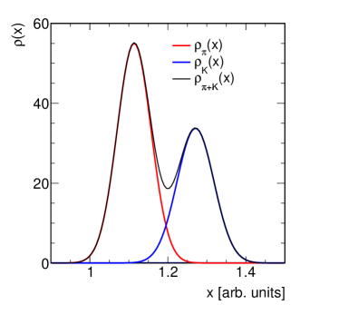
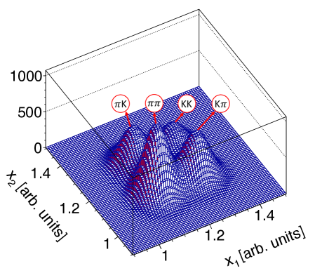
Figure 1: (Color online) Left panel: Example of the single-particle distribution $\rho(x)$ [Eq. 4] for the system of pions and kaons. Right panel: Example of the two-particle distribution $\rho(x_{1},x_{2})$ for the system of pions and kaons. The shown distribution is obtained by assuming that $x_{1}$ and $x_{2}$ are independent, i.e., $f_{ab}(x_{1},x_{2})=f_{a}(x_{1})\cdot f_{b}(x_{2})$, and pion and kaon multiplicities are uncorrelated and distributed according to Poisson distributions. The functions $f_{\pi}(x)$ and $f_{K}(x)$, and mean multiplicities of $N_{\pi}$ and $N_{K}$ correspond to those shown in the left panel.

There are two commonly used parameter estimation methods (see, e.g., Ref. Cowan:2010bz ):

1. the least-squares method (LSM),

2. the maximum likelihood method (MLM).

The application of the LSM would require binning of the data points in $x$-space. This has two important disadvantages: the binning procedure causes partial loss of the experimental information, and the binning necessary for the meaningful application of the LSM (number of entries in each bin has to be large enough) may be impossible in the case of low statistics data.

The above problems are not present in the MLM, as it allows to use the unbinned data. Therefore, in the following we will briefly introduce the MLM and the way it should be applied here. Let us start from defining the likelihood function (LF):

$$L(\mathcal{X}\leavevmode\nobreak\ |\leavevmode\nobreak\ r_{K})=\prod_{j=1}^{\mathcal{N}}F(x_{j}\leavevmode\nobreak\ |\leavevmode\nobreak\ r_{K})$$ (6)

as a joint conditional probability of the measurements $\mathcal{X}$ at the fixed value of the parameter $r_{K}$. Now, in the LF we treat the measurements $\mathcal{X}$ as fixed values and the parameter $r_{K}$ as a variable. According to the maximum likelihood principle we should choose a value of $r_{K}=r_{K}^{*}$ which maximizes $L(\mathcal{X}\leavevmode\nobreak\ |\leavevmode\nobreak\ r_{K})$. It is usually more convenient to minimize the auxiliary function, $l(\mathcal{X}\leavevmode\nobreak\ |\leavevmode\nobreak\ r_{K})$, defined as :

$$l(\mathcal{X}\leavevmode\nobreak\ |\leavevmode\nobreak\ r_{K})\equiv\leavevmode\nobreak\ -\ln\big{(}L(\mathcal{X}\leavevmode\nobreak\ |\leavevmode\nobreak\ r_{K})\big{)}=-\sum_{j=1}^{\mathcal{N}}\ln\big{(}F(x_{j}\leavevmode\nobreak\ |\leavevmode\nobreak\ r_{K})\big{)}\leavevmode\nobreak\ .$$ (7)

The search for the value of $r_{K}^{*}$, which minimizes $l(\mathcal{X}|r_{K})$, has to be done using standard numerical minimization procedures James:1975dr .

To estimate the statistical uncertainty of $r_{K}^{*}$ one should use the sub-sample Tsao:2012 and/or bootstrap methods Efron:1979 at the level of events as independent data units. It is important to stress that both methods take into account correlations between measurements of the ”mass” variable for different particles. The goodness-of-fit tests are discussed in detail in Ref. Gazdzicki:1994vj .

II.2 Mean multiplicity of particle pairs

In this subsection the PSET Identification method is considered for particle pairs. Let us start with the observation that the mean multiplicity of pairs of particles of a given type is directly related to the second moment of its multiplicity distribution. For example, the mean multiplicity of pion-pion pairs, $\langle N_{\pi\pi}\rangle$, is given as:

$$\langle N_{\pi\pi}\rangle\leavevmode\nobreak\ =\leavevmode\nobreak\ \frac{1}{2}\big{\langle}N_{\pi}\,(N_{\pi}-1)\big{\rangle}\leavevmode\nobreak\ =\leavevmode\nobreak\ \frac{\langle N_{\pi}^{2}\rangle-\langle N_{\pi}\rangle}{2}\leavevmode\nobreak\ .$$ (8)

When mean multiplicities of pions, $\langle N_{\pi}\rangle$, and pion-pion pairs, $\langle N_{\pi\pi}\rangle$, are known, the second moment of the pion multiplicity distribution can be calculated as

$$\langle N_{\pi}^{2}\rangle\leavevmode\nobreak\ =\leavevmode\nobreak\ 2\cdot\langle N_{\pi\pi}\rangle+\langle N_{\pi}\rangle\leavevmode\nobreak\ .$$ (9)

In a similar way $\langle N_{K}^{2}\rangle$ and $\langle N_{\pi}\cdot N_{K}\rangle$ are calculated. Thus the problem of measuring second moments of joint multiplicity distributions of identified particles is reduced to finding the mean multiplicities of identified particle pairs.

The experimental data on particle pairs in $M$ events is defined as follows. Number of particle pairs in an event $i$ of multiplicity $N_{i}$ is

$$N_{i}^{(2)}=\frac{1}{2}N_{i}(N_{i}-1)\leavevmode\nobreak\ .$$ (10)

The total number of pairs in all $M$ events is

$$\mathcal{N}^{(2)}=\sum_{i=1}^{M}N_{i}^{(2)}\leavevmode\nobreak\ ,$$ (11)

and the mean multiplicity of all possible pairs can be calculated as

$$\langle N^{(2)}\rangle=\frac{\mathcal{N}^{(2)}}{M}\leavevmode\nobreak\ .$$ (12)

The full set of the pair data consists of $\mathcal{N}^{(2)}$ pairs:

$$\mathcal{X}^{(2)}=\{(x_{1},x_{2})_{1},(x_{1},x_{2})_{2},\ldots,(x_{1},x_{2})_{\mathcal{N}^{(2)}}\}\leavevmode\nobreak\ .$$ (13)

The two-particle mass distribution function $\rho(x_{1},x_{2})$ is a weighted sum of two-dimensional pdfs of identified pairs:

$$\rho(x_{1},x_{2})\equiv\rho_{\pi\pi}(x_{1},x_{2})+\rho_{KK}(x_{1},x_{2})+\rho_{\pi K}(x_{1},x_{2})+\rho_{K\pi}(x_{1},x_{2})$$

$$\equiv\langle N_{\pi\pi}\rangle\cdot f_{\pi\pi}(x_{1},x_{2})+\langle N_{KK}\rangle\cdot f_{KK}(x_{1},x_{2})+\langle N_{\pi K}\rangle\cdot f_{\pi K}(x_{1},x_{2})+\langle N_{K\pi}\rangle\cdot f_{K\pi}(x_{1},x_{2})\leavevmode\nobreak\$$

$$\equiv\langle N^{(2)}\rangle\big{(}r_{\pi\pi}\cdot f_{\pi\pi}(x_{1},x_{2})+r_{KK}\cdot f_{KK}(x_{1},x_{2})+r_{\pi K}\cdot f_{\pi K}(x_{1},x_{2})+r_{\pi K}\cdot f_{K\pi}(x_{1},x_{2})\leavevmode\nobreak\ \big{)},$$ (14)

with $r_{\pi\pi}+r_{KK}+2\cdot r_{\pi K}=1$ . Consequently, only two parameters should be estimated from the experimental measurements $\mathcal{X}^{(2)}$. The two-dimensional probability density function for the system of pions and kaons reads:

$$F(x_{1},x_{2}|r_{\pi\pi},r_{KK})=r_{\pi\pi}\cdot f_{\pi\pi}(x_{1},x_{2})+r_{KK}\cdot f_{KK}(x_{1},x_{2})+r_{\pi K}\cdot f_{\pi K}(x_{1},x_{2})+r_{\pi K}\cdot f_{K\pi}(x_{1},x_{2})$$ (15)

and using the MLM the auxiliary likelihood function:

$$l(\mathcal{X}^{(2)}\leavevmode\nobreak\ |\leavevmode\nobreak\ r_{\pi\pi},r_{KK})=-\sum_{j=1}^{\mathcal{N}^{(2)}}\ln\big{(}F\left((x_{1},x_{2})_{j}\leavevmode\nobreak\ |\leavevmode\nobreak\ r_{\pi\pi},r_{KK}\right)\big{)}\leavevmode\nobreak\ .$$ (16)

is minimized to determine the parameters $r_{\pi\pi}$ and $r_{KK}$. Statistical uncertainties of the fitted parameter values, r_ππ and r_KK are to be estimated following the procedure described in the previous subsection. An example of the $\rho(x_{1},x_{2})$ function is presented in Fig.1 right.

III PSET Identification method: towards general formulation

In this section the results presented in the previous section are extended to three particle types and to third moments of the multiplicity distributions. Then, the extension to higher number of particle types and higher moments is obvious.

In the case of three particle types, for example, pions, kaons, and protons, the two-particle ”mass” distribution function reads:

$$\rho(x_{1},x_{2}) =\langle N^{(2)}\rangle\big{(}\leavevmode\nobreak\ r_{\pi\pi}\cdot f_{\pi\pi}(x_{1},x_{2})+r_{KK}\cdot f_{KK}(x_{1},x_{2})+r_{pp}\cdot f_{pp}(x_{1},x_{2})$$

$$+r_{\pi K}\cdot f_{\pi K}(x_{1},x_{2})+r_{K\pi}\cdot f_{K\pi}(x_{1},x_{2})\leavevmode\nobreak\ +r_{\pi p}\cdot f_{\pi p}(x_{1},x_{2})$$

$$+r_{p\pi}\cdot f_{p\pi}(x_{1},x_{2})+r_{Kp}\cdot f_{Kp}(x_{1},x_{2})+r_{pK}\cdot f_{pK}(x_{1},x_{2})\leavevmode\nobreak\ \big{)}\leavevmode\nobreak\ .$$ (17)

From relations $r_{ab}=r_{ba}$ and $\sum_{a,b}r_{ab}=1$ it follows that only five parameters are independent. Their values can be found by minimizing the corresponding auxiliary likelihood function, as that in Eq. (16). In a similar way expressions for more than three particle types can be obtained.

Let us now consider third moments of the multiplicity distribution for two particle types, pions and kaons. To calculate them within the PSET Identification method one should first extract from the data the mean multiplicity of identified three-particle sets. Then the three-dimensional pdfs, $f_{abc}(x_{1},x_{2},x_{3})$, have to be known. With these functions, the three-particle pdfs $F(x_{1},x_{2},x_{3}\leavevmode\nobreak\ |\leavevmode\nobreak\ r)$ can be calculated. Here $r$ denotes a set of unknown independent parameters. Their values should be fitted to the data on particle triplets

$$\mathcal{X}^{(3)}=\{(x_{1},x_{2},x_{3})_{1},(x_{1},x_{2},x_{3})_{2},\ldots,(x_{1},x_{2},x_{3})_{\mathcal{N}^{(3)}}\}\leavevmode\nobreak\ .$$ (18)

Mean multiplicities $\langle N_{abc}\rangle=r_{abc}\langle N^{(3)}\rangle$ are straightforwardly connected with the third order moments of the identified particle multiplicity distributions. For example,

$$\langle N_{\pi\pi\pi}\rangle =\frac{\langle N_{\pi}(N_{\pi}-1)(N_{\pi}-2)\rangle}{3!}=\frac{1}{6}\,\left[\,\langle N_{\pi}^{3}\rangle-3\langle N_{\pi}^{2}\rangle+2\langle N_{\pi}\rangle\,\right]\leavevmode\nobreak\ ,$$ (19)

$$\langle N_{\pi\pi K}\rangle =\frac{\langle N_{\pi}(N_{\pi}-1)N_{K}\rangle}{2}=\frac{1}{2}\,\left[\,\langle N_{\pi}^{2}N_{K}\rangle-\langle N_{\pi}N_{K}\rangle\,\right]\leavevmode\nobreak\ .$$ (20)

In this way the mean multiplicity of the identified three-particle set, $\langle N_{abc}\rangle$, is obtained by a linear combination of third, second, and first moments of the identified particle multiplicity distributions. Similarly, third moments of the multiplicity distribution can be derived from a linear combination of mean multiplicities of single particles, particle pairs, and particle triplets.

The above procedures are straightforwardly extendable to $k$-particle sets and moments of order $k$ with $k>3$ for an arbitrarily large number of particle types.

IV Test on simulated data

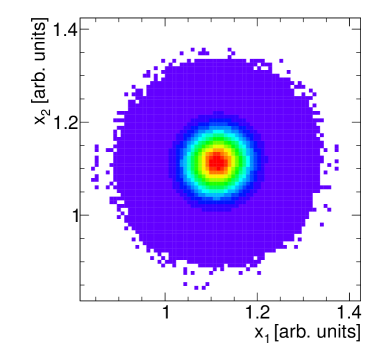
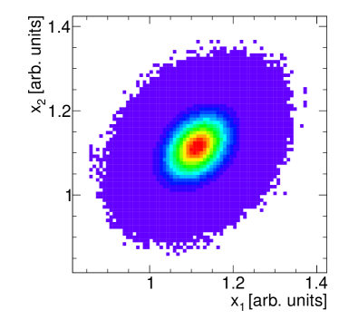
Figure 2: (Color online) Left panel: Two-particle distribution $\rho(x_{1},x_{2})$ for pions with the correlation coefficient $R$ = 0.1. Right panel: Similar to the left panel with the correlation coefficient $R$ = 0.5.

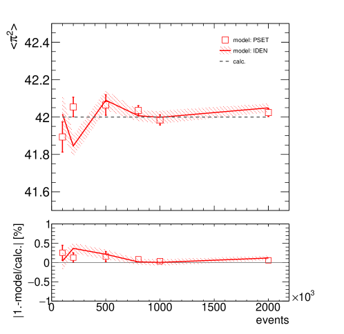
Figure 3: (Color online) Upper panel: Results for the second moments of pions as computed with the PSET method (open boxes) and the Identity method (solid lines). The value of the correlation coefficient is taken to be $R$ = 0.1 (cf. left panel of Fig. 2). The analytical calculation is represented with the dashed line. Bottom panel: The ratios of the second moments of pions as computed with the PSET method to the theoretical baseline (open boxes). Similar ratios for the Identity method are presented with the solid lines.

Figure 4: (Color online) Upper panel: Results for the second moments of pions as computed with the PSET method (open boxes) and the Identity method (solid lines). The value of the correlation coefficient is taken to be $R$ = 0.5 (cf. right panel of Fig. 2). The analytical calculation is represented with the dashed line. Bottom panel: The ratios of the second moments of pions as computed with the PSET method to the theoretical baseline (open boxes). Similar ratios for the Identity method are presented with the solid lines.

In this section, based on simulated data, we provide results of the PSET Identification method and confront them with those obtained with the Identity method. Although the method is general and functions for unlimited number of particle species, for simplicity we consider the case of two particle types only. The simulation process consists of the following steps: (i) from independent Poisson distributions, with a given means of $\lambda_{\pi}=6$ and $\lambda_{K}=4$, we first randomly generate multiplicities of pions and kaons in each event; (ii) using the $\rho_{\pi}$ and $\rho_{K}$ distributions functions, presented in the left panel of Fig. 1 we generate the values of the particle identification variable $x$ corresponding to each particle species. In order to introduce correlations between pairs of $x$ quantities, we use the probability density function of the bi-variate normal distribution

$$f(x_{1},x_{2})=\frac{1}{2\pi\sqrt{|\Sigma|}}e^{-0.5\left(\mathbf{x}-\mathbf{\langle x\rangle}\right)^{T}\Sigma^{-1}\left(\mathbf{x}-\mathbf{\langle x\rangle}\right)},$$ (21)

where $|\Sigma|$ is the determinant of $\Sigma$. The column vectors $\mathbf{x}$, $\mathbf{\left<x\right>}$ and the covariance matrix $\Sigma$ are defined as

$$\mathbf{x}=\begin{pmatrix}x_{1}\\ x_{2}\end{pmatrix},\mathbf{\langle x\rangle}=\begin{pmatrix}\langle x_{1}\rangle\\ \langle x_{2}\rangle\end{pmatrix},\Sigma=\begin{pmatrix}\sigma_{x_{1}}^{2}&R\sigma_{x_{1}}\sigma_{x_{2}}\\ R\sigma_{x_{1}}\sigma_{x_{2}}&\sigma_{x_{2}}^{2}\end{pmatrix}.$$ (22)

The dimensionless parameter $R$, referred to as the correlation coefficient, is introduced as

$$R=\frac{\left<(x_{1}-\left<x_{1}\right>)(x_{2}-\left<x_{2}\right>)\right>}{\sigma_{x_{1}}\sigma_{x_{2}}}.$$ (23)

We further note that the correlations between $x_{1}$ and $x_{2}$ are introduced only if they belong to the same particle, otherwise they are generated independently, i.e., the value of the correlation coefficient $R$ is set to zero in this case. Each generated $i$th event contains a set of quantities $X=\{x_{1},x_{2},...,x_{N_{i}}\}$, where $N_{i}$ refers to the total number of pions and kaons in a given event. Next, we construct all possible two-particle pairs $(x_{1},x_{2})$ of the $x$ quantity inside a given event. The full set of these pairs in all events (cf. Eq. 13) generates an inclusive two particle mass distribution. From Eq. 9 we estimate second moments of pions. In doing so, we first fit the two-dimensional mass distribution (cf. the right panel of Fig. 1) and use Eq. II.2 to determine the mean numbers of pion-pion pairs $N_{\pi\pi}$. In a similar way we compute the second moments of the kaon multiplicity distribution. For clarity we present the results for pions only. In Fig. 2 the two-particle distributions $\rho(x_{1},x_{2})$ are presented, where the left and right panels correspond to different values of the correlation coefficient: $R$ = 0.1 and 0.5 respectively. The corresponding reconstructed second moments are presented in the upper panels of Figs. 3 and 4, where open boxes represent the results from the current study (PSET Identification method) while the solid lines are obtained with the Identity method Arslandok:2018pcu . In the bottom panels of Figs. 3 and 4 the ratios of the second moments of pions to their theoretical values are presented. Close inspection of Figs. 3 and 4 indicates that with the increasing correlations between $x_{1}$ and $x_{2}$ the Identity method deviates from the theoretical baseline, while the PSET Identification method, as expected, is protected against such correlations. We further note that, the amount of bias in the Identity method depends on mean multiplicities, number of involved particle species etc.

V Summary

The paper presents a new method, the Particle-Set Identification method, for reconstructing moments of multiplicity distribution of identified particles. A PSET represents a set of particles which is constructed from particles created in a collision. Mean multiplicities of particle sets of a given type are extracted from the measurements of the multi-dimensional distribution of a particle ”mass” variable. This multi-dimensional distribution is used to calculate moments of the joint multiplicity distributions of identified particles.

First, the PSET Identification method is introduced for the simple case of two particle types, addressing first and second order moments. Then a sketch of the generalization of the method is presented for $k$-particle sets and moments of order $k\geq 3$ for the case of an arbitrary number of particle types.

Finally, using a simple model we explicitly demonstrated that the PSET Identification method is protected against possible correlations in the multi-dimensional distribution of the particle ”mass” variables.

The PSET Identification method has a broader range of applicability than the Identity method introduced by us previously to solve the problem of incomplete particle identification. Particularly, it does not assume that measurements of particle ”mass” for different particles are independent. The issue of introducing momentum dependent pdfs within the PSET identification method is left for future studies.

- (1) V. Koch, “Hadronic Fluctuations and Correlations,” in Relativistic Heavy Ion Physics (R. Stock, ed.), pp. 626–652, Springer-Verlag Berlin Heidelberg, 2010.
- (2) M. Gazdzicki and P. Seyboth, “Search for Critical Behaviour of Strongly Interacting Matter at the CERN Super Proton Synchrotron,” Acta Phys. Polon., vol. B47, p. 1201, 2016.
- (3) M. Gazdzicki, K. Grebieszkow, M. Mackowiak, and S. Mrowczynski, “Identity method to study chemical fluctuations in relativistic heavy-ion collisions,” Phys. Rev., vol. C83, p. 054907, 2011.
- (4) M. I. Gorenstein, “Identity Method for Particle Number Fluctuations and Correlations,” Phys. Rev., vol. C84, p. 024902, 2011. [Erratum: Phys. Rev.C97,no.2,029903(2018)].
- (5) A. Rustamov and M. I. Gorenstein, “Identity Method for Moments of Multiplicity Distribution,” Phys. Rev., vol. C86, p. 044906, 2012.
- (6) C. A. Pruneau, “Identity method reexamined,” Phys. Rev., vol. C96, no. 5, p. 054902, 2017.
- (7) C. A. Pruneau and A. Ohlson, “Differential Correlation Measurements with the Identity Method,” Phys. Rev., vol. C98, no. 1, p. 014905, 2018.
- (8) M. Mackowiak-Pawlowska and P. Przybyla, “Generalisation of the identity method for determination of high-order moments of multiplicity distributions with a software implementation,” Eur. Phys. J., vol. C78, no. 5, p. 391, 2018.
- (9) T. Anticic et al., “Phase-space dependence of particle-ratio fluctuations in Pb + Pb collisions from 20 A to 158 A GeV beam energy,” Phys. Rev., vol. C89, no. 5, p. 054902, 2014.
- (10) M. Mackowiak-Pawlowska, “Energy Dependence of Identified Hadron Fluctuations in p + p Interactions from NA61/SHINE,” PoS, vol. CPOD2013, p. 048, 2013.
- (11) S. Acharya et al., “Relative particle yield fluctuations in Pb-Pb collisions at TeV,” Submitted to: Eur. Phys. J., 2017.
- (12) A. Rustamov, “Net-baryon fluctuations measured with ALICE at the CERN LHC,” Nucl. Phys., vol. A967, pp. 453–456, 2017.
- (13) M. Gazdzicki, “Statistical tool for particle ’identification’ by ’mass’ measurement,” Nucl. Instrum. Meth., vol. A345, pp. 148–155, 1994.
- (14) G. Cowan, “Topics in statistical data analysis for high-energy physics,” in High-energy physics. Proceedings, 17th European School, ESHEP 2009, Bautzen, Germany, June 14-27, 2009, pp. 197–218, 2013. [,207(2013)].
- (15) F. James and M. Roos, “Minuit: A System for Function Minimization and Analysis of the Parameter Errors and Correlations,” Comput. Phys. Commun., vol. 10, pp. 343–367, 1975.
- (16) M. Tsao and X. Ling, “Subsampling Method for Robust Estimation of Regression Models,” Open Journal of Statistics, vol. 2, pp. 281–296, 2012.
- (17) B. Efron, “Bootstrap methods: Another look at the jackknife,” The Annals of Statistics, vol. 7, pp. 1–26, 1979.
- (18) M. Arslandok and A. Rustamov, “TIdentity module for the reconstruction of the moments of multiplicity distributions,” Nucl. Instrum. Meth., vol. A946, p. 162622, 2019.