Multi timescale bandwidth profile and its application for burst-aware fairness

Abstract

We propose a resource sharing scheme that takes into account the traffic history over several predefined time scales and provides fair resource sharing considering the traffic history. Our concept builds on a simplified version of core-stateless resource sharing, where we only use a few Drop Precedences (DPs). For packet marking we introduce Multi timescale bandwidth profile. Additionally, we provide basic dimensioning concepts for the proposed schema and present its simulation based performance analysis.

I Introduction

Quality of Service (QoS) is a fundamental area of networking research that has been researched for a long time. Despite this several open issues remain as collected in [1]. Per node (e.g. per subscriber or per traffic aggregate) fairness, being one of these, is usually provided by per node WFQ, but that does not scale as the number of node increases. Core-stateless schedulers [2, 3, 4] solve this, but they still only provide fairness on a single timescale, typically at the timescale of round-trip time (RTT). These solutions mark packets per node at the edge of the network and do simple, session-unaware scheduling in the core of the network based on the marking. The most common way to provide fairness on longer timescales is to introduce caps, e.g. a monthly cap on traffic volume, however the congestion lasts much shorter time period. A similar attempt is to limit the congestion volume instead of the traffic volume as described in [5, 6]. The need for fairness on different time scales is illustrated by the example of short bursty flows and long flows, as mice and elephants in [7]. A demand in this area is that a continuously transmitting node shall achieve the same long term average throughput as nodes with small/medium bursts now and then.

Traffic at the same time is becoming more and more bursty, including traffic aggregates, due to the highly increased throughput of 5G Base Stations [8]. When deploying mobile networks, operators often lease transport lines as Mobile Backhaul from the Core Network to the Base Stations. The transport services and related bandwidth profiles defined by the Metro Ethernet Forum (MEF) [9] are most commonly used for this purpose today. However using the current service definitions, it is not possible to achieve per node (per transport service in this case) fairness and good utilization simultaneously and also it only takes into account a small timescale, i.e. the instantaneous behavior.

In this paper we propose a resource sharing scheme that takes into account the traffic history of nodes over several predefined timescales and provides fair resource sharing based on that. Our concept builds on a simplified version of core-stateless resource sharing, where we only use a few Drop Precedences.

II Packet level behavior

In this section, we extend the Two-Rate, Three-Color Marker (trTCM) to provide fairness on several timescales and show how we apply core stateless scheduling on the marked packets.

II-A Packet Marking

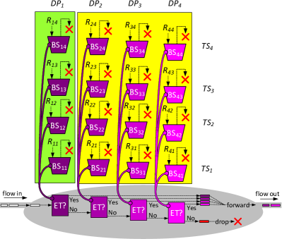
Figure 1: trTCM bandwidth profile for a single priority

Figure 2: A $4\times 4$ Multi Timescale Bandwidth Profile

MEF currently uses flavors of trTCM for bandwidth profiling [9]. The simplest case, when a single priority is used and there is no token sharing or color awareness, is depicted on Fig. 2. It has two rate parameters, the guaranteed Committed Information Rate (CIR) and the non-guaranteed Excess Information Rate (EIR). Both has an associated token bucket (Committed Burst Size (CBS) and Excess Burst Size (EBS)), whose sizes are typically set to $CBS\approx CIR\times RTT$ and $EBS\approx EIR\times RTT$, where $RTT$ denotes the round trip time. A packet is marked green (conform to CIR), yellow (conform to EIR) or dropped (red) based on the amount of tokens in the associated token buckets. A bucket must contain at least as many tokens as the packet size, marked as Enough Tokens (ET?). If a packet is marked a given color, that many tokens are removed from the relevant bucket.

We extend the trTCM by increasing the number of colors (i.e. drop precedences (DPs)) and by introducing multiple token buckets per drop precedence, representing different timescales (TSs). An example for this Multi Timescale Bandwidth Profile (MTS-BWP) is shown on Fig 2, where the number of DPs is $N_{DP}=4$ and the number of TSs is $N_{TS}=4$.

The darkest purple color (DP 1) is similar to green in the sense that we intend to guarantee transmission of packets marked dark purple. The lighter colors are similar to yellow, though we intend to provide a more refined service for them than simple non-guaranteed delivery. The token rate of the bucket associated with drop precedence $dp$ and timescale $ts$ is $R_{dp,ts}$ and the bucket size of BS_dp,ts is set to $BS_{dp,ts}\approx R_{dp,ts}\times TS_{ts}$. An example time scale vector with $N_{TS}=4$ is $TS=\{TS_{1},\ldots,TS_{4}\}=\{0.1,1,10,100~{}\textrm{sec}\}$, where we assume that $TS_{1}$ is in the order of magnitude of the typical RTT.

That is, $\mbox{\boldmath$R$}=\{R_{dp,ts}\}$ and $\mbox{\boldmath$BS$}=\{BS_{dp,ts}\}$ are matrices of size $N_{DP}\times N_{TS}$. A packet can be marked a given DP value $dp$ if all buckets BS${}_{dp,ts},\ \forall ts\in\{1,\ldots,N_{TS}\}$ (which we shorthand as $\forall ts$) contain enough tokens. Upon successful marking all respective buckets are decreased with the packet size.

If we want to enable more bursty traffic on lower timescales, we have to offer smaller bandwidth on higher timescales. Thus the rows of $R$ are monotonically decreasing, i.e.

$$R_{dp,ts+1}\geq R_{dp,ts},\ \forall dp,ts.$$ (1)

II-B Active Queue Management (AQM) algorithm

We assume a FIFO buffer with drop the largest DP from head AQM. More precisely when the buffer is full, we determine the largest DP which has packet present in the buffer and drop the first packet from the head which has this DP.

This algorithm can be implemented efficiently by applying the AQM in [3] for 4 DPs.

This behavior can also be approximated on existing hardware by representing drop precedences with DSCPs; configuring these DSCPs to the same queue; and configuring DP specific TailDrop thresholds to drop the different DPs at increasing queue lengths (the largest DP at the smallest queue length) [10].

III Fluid model of MTS-BWP

We analyze the performance of MTS-BWP in a fast and simple fluid simulator, because our focus is not the packet level behavior and the interaction of congestion control and scheduling, as there is other work focusing on that, e.g. [11]. Rather we are interested in how the newly introduced bandwidth profile can provide fairness on several timescales, when the system is ideal, i.e.  the used congestion control can utilize its share instantaneously and with no packet loss.

III-A High level model

We model a common bottleneck shared among several nodes with identical BWP configuration. A node may have one or several active flows. When no BWP is applied, nodes share the bottleneck proportionally to the number flows within the nodes. The applied BWP constraints this allocation, all traffic with DP above congestion DP is transmitted and with DP below is discarded. Bandwidth allocation within the congestion DP is still proportional with the number of flows. DPs signify priority in the sense that whenever congestion occurs the transmission on higher DPs (i.e., traffic marked with higher DP value) is reduced first.

The token level $TL^{n}_{dp,ts}(t)$ in bucket $\textrm{BS}_{dp,ts}$ of node $n$ is maintained and fluid flows out from each bucket of a given DP according to the transmission rate of the node on that DP $th_{dp,n}$.

Our ideal system model (istantenous adaptation, no packet loss) assumes no bottleneck buffer and 0 RTT. Consequently we set $BS_{dp,1}=0$ in the fluid simulator (which results in maximum fluid rate of $R_{dp,1}$ on a given $dp$, see Eq. 2).

III-B Simulator model

III-B1 System parameters

The system is described by the following parameters:

• $C$: the total service capacity;

• $N$: the number of nodes;

• $\mbox{\boldmath$R$},\mbox{\boldmath$BS$}$ (assumed to be the same for all nodes);

• $f^{\max}$ flow limit: the maximum number of concurrent active flows at each node; further flows are discarded upon arrival.

III-B2 Traffic Model

We use a compound Poisson point process with a discrete file sizes distribution (given by possible file sizes and associated probabilities) as an input, and based on that we simulate the arrival time and the size of each arriving flow for each node.

Each node has a nominal speed $S_{n}$ in all investigated situations, we will stick to the natural choice of $S_{n}=C/N,\,n=1,\dots,N$. The nominal load of each node can then be calculated as

$$\textrm{nominal load}=\textrm{average file size}\times\textrm{arrival rate}/S_{n}.$$

The system load is the average of the nominal loads for all nodes. The system is underloaded if its load is less than 1, and it is overloaded otherwise. A node has low load if its nominal load is less than the system load, and it has high load otherwise.

III-B3 Discrete event simulator

A discrete event simulator runs a simulation using a given traffic input (arrival time and file size series) for a given set of system parameters. The simulator identifies the following events:

1. flow arrival,

2. flow finishing,

3. a token bucket emptying,

and keeps track of the following values:

1. simulation time;

2. list of active flows;

3. remaining size of each active flow;

4. token bucket levels, $TL^{n}_{dp,ts}$.

These variables are sufficient to determine the time and type of the next event and the current bandwidth allocation which applies until the next event. The simulator then proceeds to the next event, updates all information and iterates this loop.

Once finished, the simulator provides the following information as an output:

1. list of all event times (including flow arrivals and departures);

2. list of the bandwidth allocation for each node and each DP between events;

3. flow count for each node at each event time.

III-C Bandwidth allocation model

At any given point in time, we collect the throughput bounds determined by the current bucket levels for a drop precedence $dp$ at node $n$ into a $N_{DP}\times N$ matrix, denoted by $B\!D$, whose elements are

$$\min_{ts=1\dots N_{TS}}\{R_{dp,ts}:TL^{n}_{dp,ts}=0\}.$$ (2)

To present the bandwidth allocation we need the following notation:

• $f_{n}$ is the number of flows in node $n$,

• $th_{n}$ is the throughput of node $n$, initialized with 0,

• $e_{n}$ shows that node $n$ is eligible for increase, initialized with True.

The iterative algorithm to calculate the bandwidth allocation is as follows.

The congestion DP is calculated as

$$dp_{c}=\min\Big{\{}i:\sum_{dp=1}^{i}\sum_{n=1}^{N}B\!D_{dp,n}\geq C\Big{\}}.$$

$th_{n}$ is initialized for all $n$ as

$$th_{n}=\sum_{dp=1}^{dp_{c}-1}B\!D_{dp,n}.$$

Then the procedure iterate the following 3 steps until $\sum_{n=1}^{N}th_{n}=C$:

1. Nodes with $th_{n}=\sum_{dp=1}^{dp_{c}}B\!D_{dp,n}$ are set to non-eligible ($e_{n}=$ False.)

2. Mark all eligible nodes for which the ratio $th_{n}/f_{n}$ is minimal among all eligible nodes.

3. Increase $th_{n}$ for all marked nodes by $f_{n}\cdot\delta$, where $\delta>0$ is calculated as the maximal possible increase such that the following remain valid:

   • $th_{n}\leq\sum_{dp=1}^{dp_{c}}B\!D_{dp,n}$ for all $n$,

   • the ratio $th_{n}/f_{n}$ from among all marked nodes does not increase beyond the second smallest ratio $th_{n}/f_{n}$ from among all eligible nodes, and

   • $\sum_{n=1}^{N}th_{n}\leq C$.

From $th_{n}$ and $BD_{dp,n}$ calculating the per DP throughput $th_{dp,n}$ is straightforward.

IV Dimensioning guidelines

This section focuses on the dimensioning of the token rate matrix $R$ and the token bucket size matrix $BS$ (defined in Section II-A). Proper dimensioning of $R$ and $BS$ are vital to obtain the desired properties of the bandwidth profile. We consider a system with $N$ nodes with identical MTS-BWP configuration over a bottleneck link with capacity $C$. The required properties are the following:

1. there are $N_{f\!s}$ predefined download speeds $BW_{1},BW_{2},\dots,BW_{N_{f\!s}}$ (decreasing) provided for files of sizes $f\!s_{1},f\!s_{2},\dots,f\!s_{N_{f\!s}}$ (increasing) arriving at a previously inactive node ($BW_{1}$ is also the peak rate provided to a node after an inactive period);

2. provide the nominal speed $S_{n}=C/N$ to each node in long-term average;

3. ensure $BW_{N_{f\!s}}>S_{n}$;

4. provide the minimum guaranteed speed $G_{1},G_{2},\dots,G_{N_{TS}}$ (decreasing) in case of $TL^{n}_{11}=0,TL^{n}_{12}=0,\dots,TL^{n}_{N_{TS}=0}$ respectively;

5. guarantee work conserving property (i.e. when there is traffic, the full link capacity shall be used).

In the following analysis we focus on the $N_{DP}=4$ and $N_{TS}=4$ case, which allows for $N_{f\!s}=N_{TS}-1=3$ file sizes with predefined downloads speeds, but it is straightforward to generalize for $N_{TS}>4$. We aim to minimize $N_{DP}$ and will settle at $N_{DP}=4$, providing insight to how the 4 DPs are used as well as what happens for fewer DPs.

IV-A Token rate matrix $R$

In this part we present a simple dimensioning method for a $4\times 4$ matrix $R$ based on the requirements 1–5 above. All rows of $R$ should be decreasing according to (1).

We use the following intuitive guidelines for $R$:

• DP 1 is used for the guaranteed speeds $G_{1},G_{2},\dots$ and not intended to be the limiting DP;

• DP 1 and 2 are used to be able to reach the predefined download speeds ($BW_{1},BW_{2},\dots$) by a low load node in situations when most nodes are on $ts=N_{TS}$;

• DP 3 or 4 is the congestion DP for high load nodes while low load nodes are inactive;

• DP 4 is used to guarantee the work conserving property.

In accordance with these guidelines, we propose the structure

$$\mbox{\boldmath$R$}\!=\!\!\begin{bmatrix}G_{1}&G_{2}&G_{3}&G_{4}\\ BW_{1}\!-\!G_{1}&BW_{2}\!-\!G_{2}&BW_{3}\!-\!G_{3}&\frac{C-BW_{1}}{N-1}\!-\!G_{4}\\ *&*&*&S_{n}\!-\!\frac{C-BW_{1}}{N-1}\\ C&C&C&C\end{bmatrix}$$

The first row (DP 1) is straightforward and simply implements the guaranteed speeds. Note that $G_{1}\leq S_{n}$ needs to hold to avoid congestion on DP 1.

$R_{2,1}$ is calculated so that $R_{1,1}+R_{2,1}=BW_{1}$ to ensure the predefined download speed $BW_{1}$ on DP 1 and 2; similarly, $R_{2,2}=BW_{2}-R_{2,1}$ and $R_{2,3}=BW_{3}-R_{3,1}$.

Our next remark is that $R_{3,4}$ is defined so that

$$R_{1,4}+R_{2,4}+R_{3,4}=S_{n}$$ (4)

holds; this important property will be called the return rule. First note that if $R_{1,4}+R_{2,4}+R_{3,4}\leq S_{n}$, then any node $n$ with nominal load larger than 1 will continue to deplete their token buckets and eventually end up with

$$TL^{n}_{1,N_{TS}}=TL^{n}_{2,N_{TS}}=TL^{n}_{3,N_{TS}}=0.$$ (5)

Actually, (5) is exactly the way bad history is described within the system.

The return rule (4) provides two important guarantees: in long-term average, only bandwidth $S_{n}$ is guaranteed on DP1–DP3 for any node $n$, but since $S_{n}=C/N$, this also means that no node will be “suppressed” in long-term average by the other nodes.

Also, over a time period when all other nodes $n$ are either inactive or have bad history as in (5), any node $\bar{n}$ with nominal load less than $1$ will eventually have $TL^{\bar{n}}_{3,4}>0$, and thus potentially have access to a rate larger than $S_{\bar{n}}$ (the node returns from “bad history” to “good history”, hence the name of the rule). The general form of the return rule would be that there exists a $dp_{r}$ such that $\sum_{dp=1}^{dp_{r}}R_{dp,N_{TS}}=S_{n}$.

Next up is $R_{2,4}$, which is defined so that

$$(N-1)(R_{1,4}+R_{2,4})+BW_{1}=C.$$

This will ensure that in the case when a single node becomes active while all other nodes are either inactive or have bad history as in (5), the congestion DP will change to 2, with the single active node having rate $BW_{1}$ and other nodes having rate $(R_{1,4}+R_{2,4})$ allocated.

The last row guarantees the work conserving property: as long as at least one node is active, it has access to the entire capacity $C$.

Finally, the system is relatively insensitive to the exact values of the elements marked with an $*$ since typically other elements will limit the bandwidth: high load nodes have a bad history and thus are limited by $R_{.,4}$, while targets for low load nodes are realized on DPs 1 and 2 and are thus limited by $(R_{1,.})$ and $(R_{2,.})$. Elements marked with an * can be selected arbitrarily as long as row 3 of $R$ is decreasing.

Further remarks: The file sizes for the predefined download speeds only affect the bucket size matrix $BS$, detailed in the next subsection. For typical choices of the parameters, the rows of $R$ are monotonically decreasing, but in case they are not, $R$ needs to be adjusted, which we neglect here. More (or fewer) timescales can be introduced in a straightforward manner to accommodate more (or fewer) predefined file sizes and download rates. In case of fewer DPs, we need to choose:

• Omitting the first row of $R$ results in no strictly guaranteed speeds.

• Omitting the second row removes the predefined download speeds, resulting in a system very similar to trTCM, with nearly no memory.

• Omitting the third row violates the return rule.

• Omitting the last row results in a non-work-conserving system, where it may occur that their previous history limits nodes to the point where less than the available capacity is used.

Example 1.

For the parameters $N=5$, $C=10$ (Gbps), guaranteed speeds $G_{1}=G_{2}=G_{3}=2,G_{4}=0.75$ (Gbps), file sizes are $f\!s_{1}=0.1,f\!s_{2}=1,f\!s_{3}=11.25$ (GByte) and download speeds $BW_{1}=6,BW_{2}=4,BW_{3}=3$ (Gbps), the following $4\times 4$ matrix is suitable:

$$\mbox{\boldmath$R$}=\begin{bmatrix}2&2&2&0.75\\ 4&2&1&0.25\\ 10&10&1&1\\ 10&10&10&10\end{bmatrix}$$ (6)

IV-B Bucket size matrix $BS$

The sizes of the buckets are calculated from the rates in $R$ and the list of timescales $TS$, which we define as

$$TS=[0,f\!s_{1}/BW_{1},f\!s_{2}/BW_{2},f\!s_{3}/BW_{3}].$$ (7)

$TS_{1}=0$ represents the ideal behavior of the fluid model. The remaining timescales correspond to download times of the predefined file sizes. We use the last timescale ($TS_{4}$) to define how long a node must send with bandwidth at least $S_{n}$ to be considered to have bad history. In Example 1, we actually set $TS_{4}=30$ sec (to allow a 30 second active period, before a node is considered to have bad history) and calculate $f\!s_{3}$ accordingly.

We set the bucket sizes according to the formula

$$BS_{dp,ts}=$$ (8)

$$\left\{\begin{array}[]{lrl}0\hfill&\mbox{for }ts=1\\ TS_{2}(R_{dp,1}-R_{dp,2})&\mbox{for }ts=2\\ \sum_{k=2}^{ts}(TS_{k}-TS_{k-1})(R_{dp,k-1}-R_{dp,ts})&\mbox{for }ts>2\end{array}\right.$$ (12)

which will result in a previously inactive node emptying bucket $\textrm{BS}_{dp,ts}$ after time $TS_{ts}$ (assuming the rate at DP $dp$ is limited only by the node’s own history and not by other nodes), taking into account the fact that it uses different bandwidth on different timescales. Buckets with $BS_{dp,ts}=0$ act as rate limiters in the fluid model, due to Eq. 2.

Note that when using the above $R$ and $BS$ dimensioning method, the flow throughput of a single flow of size $f\!s_{2}$ can reach as high as

$$BW^{\prime}_{2}=\frac{TS_{2}\cdot BW_{1}+(TS_{3}-TS_{2})\cdot BW_{2}}{TS_{3}}\geq BW_{2}.$$ (13)

If one wants to replace the current maintainable download speed requirement to a flow throughput requirement for $f\!s_{2}$, $BW_{2}$ in (IV-A) should be replaced by the (slightly smaller) solution of Eq. (13) for $BW_{2}$ when setting the left-hand side equal to the flow throughput requirement. For Example 1, and for the anticipated meaningful input values, the difference between $BW_{2}$ and $BW^{\prime}_{2}$ is very small; specifically, $BW_{2}^{\prime}=4.1333$ (Gbps).

Also note that the above calculations are for the fluid model; for actual packet-based networks, bucket sizes $BS^{*}_{dp,ts}$ must have a minimum: at least MTU (maximum transmission unit) to be able to pass packets, and they must also be able to allow bursts on the RTT timescale. In summary,

$$BS^{*}_{dp,ts}=\max(BS_{dp,ts},\,MTU,\,R_{dp,ts}\cdot RTT).$$

V Simulation

V-A Simulation parameters

In all simulations, the MTS-BWP rates ($R$), bucket sizes $BS$ and the system parameters are set according to Example 1. In the input process, we use the file sizes $f\!s_{1}$ and $f\!s_{2}$ from Example 1 with identical $50\%$ probability. $f^{\max}=20$ is for each node.

We have two groups of nodes with identical nominal loads within a group. We specify the nominal load for low load nodes (low load) and the system load, and calculate the nominal load for high load nodes using the equations in Section III-B2. The simulation setups are summarized in Table I, with the number and load of each node type varying for a total of $2\times 10+2\times 6$ actual setups.

Setup	$N_{\textrm{low}}$	$N_{\textrm{high}}$	low load	system load
A	1	4	0.5	0.6, 0.7, 0.8, 0.9, 0.95,
B	2	3		1.0, 1.1, 1.2, 1.5, 2.0
C	1	4	0.5, 0.6, 0.7,	1.1
D	2	3	0.8, 0.9, 0.95

TABLE I: Simulation setups and parameters

V-B Example simulation

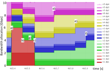
Figure 3: Example of bandwidth allocation over time

Figure 3 depicts the evolution of the bandwidth allocation in a time interval for setup A with system load of $0.95$. Colors correspond to nodes and shades within a color correspond to DPs. Node 1 (red) is the low load node. Some events are also marked (a)–(g).

Node 1 is inactive in the beginning, and the congestion DP is 3. Then a large flow starts in node 1 (a) and the congestion DP changes to 2. Node 1 starts using 2 Gbps ($R_{1,1}$) + 4 Gbps ($R_{2,1}$) of the available capacity on DP 1 and 2 respectively, while nodes 2–5 start using 0.25 Gbps ($R_{1,4}$) + 0.75 Gbps ($R_{2,4}$) respectively. ($R_{1,1}$ and $R_{2,1}$ was dimensioned for exactly this case; while the congestion DP is 2, all traffic on DP 2 can be transmitted.)

As time progresses, the buckets $\textrm{BS}_{2,2}$ and $\textrm{BS}_{1,2}$ of node 1 becomes empty (b), and the bandwidth share of node 1 drops accordingly to 2 Gbps ($R_{1,2}$) + 2 Gbps ($R_{2,2}$). The congestion DP switches back to 3, but DP 3 is dominated by nodes 2–5, because those nodes have high numbers of flows, while node 1 has only a single flow. That single large flow can still achieve $BW_{2}$ throughput as dimensioned.

Once node 1 finishes its flow (c), the available bandwidth is reallocated to nodes 2–5 on DP 3. Then, buckets which were filled previously (specifically BS_3,4) of nodes 2–5 empty one by one, and their bandwidth shares on DP 3 drop accordingly: first for node 5 (d), then node 4 (e), then node 3 (f). The exact order depends on the bucket levels of $B_{3,4}$ of each node, which depend on their earlier history, not visible in the example time interval.

In the meantime, new flow arrivals and finished services at nodes 2–5 may occur and cause minor changes in the bandwidth allocation, e.g. a flow at node 2 finishes at (g).

V-C Statistical results

Based on the simulator output, we calculate the following two statistics: the node bandwidth for active periods (periods when there is no flow at the respective node are excluded); and the flow bandwidth for the different flow sizes, which is the flow size divided by the download time. For both we plot average, 10% best and 10% worst cases, the error bars displaying the worst $10\%$–best $10\%$ interval, with a dot marking the average. Averaging and percentiles are weighted according to time for node throughputs, while they are weighted according to the number of flows for flow throughputs. All statistics are evaluated for a 1-hour run (with an extra initial warm-up period excluded from the statistics).

We compare the suggested MTS-BWP with matrix $R$ versus trTCM profile (CIR=$S_{n}$=2 Gbps, EIR=$C-S_{n}$=8 Gbps) as baseline for various setups.

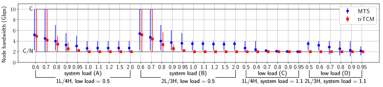
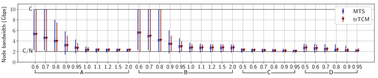
Figure 4: Node bandwidth for low load nodes for trTCM vs. MTS BWP

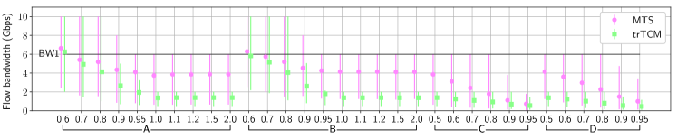
Figure 5: Node bandwidth for high load nodes for trTCM vs. MTS BWP

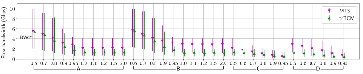
Figure 6: Flow bandwidth for small flows (100 MB) at low load nodes for trTCM vs. MTS BWP

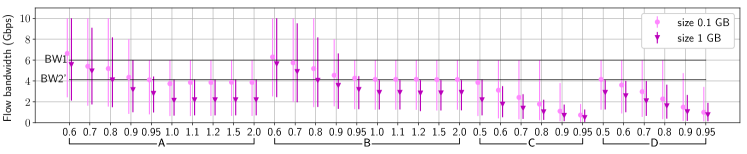
Figure 7: Flow bandwidth for large flows (1 GB) at low load nodes for trTCM vs. MTS BWP

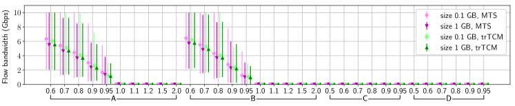
Figure 8: Flow bandwidth for small flows vs. large flows at low load nodes for MTS BWP

Figure 9: Flow bandwidth for small vs. large flows at high load nodes for trTCM vs. MTS BWP

Figure 9 displays node bandwidth statistics for low load nodes for trTCM vs. MTS. MTS consistently outperforms trTCM in allocating more bandwidth to low load nodes. The average bandwidth for MTS is higher in every scenario, and the best possible case (best $10\%$ values) is also significantly higher in most scenarios. MTS provides the most improvement in scenarios where the system is overloaded, for small system loads trTCM also performs well.

Low load node(s) perform better in the 2L/3H setup than in the 1L/4H setup, because $R$ protects a low load node better from 3 high load nodes than from 4. Finally, as the load of the low load node approaches 1, the difference between trTCM and MTS gradually disappears.

Figure 9 displays the same statistics for high load nodes. The most important observation here is that the considerable gain for low load nodes in Figure 9 comes at virtually no cost to high load nodes: the difference between the average bandwidth for high load nodes for trTCM vs. MTS BWP is negligible. The reason is that while traffic from low load nodes is indeed served faster, but the total amount of traffic served from low load nodes is the same. This means that for high load nodes, which are active longer, the effect on node bandwidth is negligible, especially for the average. (It matters little whether we decrease the same amount of bytes in a big burst or for a longer period with smaller bandwidth.)

Next we examine the prioritization of small flows ($f\!s_{1}$) vs. large flows ($f\!s_{2}$) provided by MTS-BWP compared to trTCM BWP. Figure 9 shows flow bandwidth statistics for small flows in low load nodes. MTS outperforms trTCM in allocating more bandwidth in these cases for every setup, but particularly for overloaded systems, where the difference is huge, both for average and also for best $10\%$ values. Also, as the low load is approaching 1, the difference between trTCM and MTS diminishes (just as for the node bandwidth, see Figure 9), but that is as it should be. Also, for MTS BWP, the best $10\%$ values for small flows reach $BW_{1}$ for all scenarios where the low load is below $0.9$.

Figure 9 displays the same statistics for large flows (1 GB) at low load nodes. Again, MTS outperforms trTCM significantly. The best $10\%$ throughput matches $BW_{2}^{\prime}$ and is close to the dimensioned $BW_{2}$ (see Section IV-A).

Figure 9 compares flow bandwidth statistics for small vs. large flows at low load nodes for MTS-BWP. It can be seen that small flows are successfully prioritized in all cases.

Finally, Figure 9 displays flow bandwidth at high load nodes for both small and large flows; and for both policies. There is a sharp distinction between underloaded systems and overloaded systems: for underloaded systems, even at high load nodes, typically there are only very few active flows at the same time, resulting in relatively large flow bandwidths. However, as the system load approaches 1, the per flow bandwidth drops gradually, and for overloaded systems, the number of flows in high load nodes is always close to the limit $f^{\max}=20$. Thus the flow bandwidth in high load nodes is typically close to $S_{n}/f^{\max}$, which is very sensitive to the parameter $f^{\max}$. For these nodes, we consider the node bandwidth to be a more informative statistics.

VI Conclusion

We have shown that the proposed Multi Timescale Bandwidth Profile can extend fairness from a single timescale to several timescales. We provided a dimensioning method to deploy Service Level Agreements based on MTS-BWP, which can provide target throughputs for a group of nodes. The presented tool can differentiate between nodes using the same service depending on their characteristics.

Our simulation results showed the differences in network throughput for low load and high load nodes. There were high throughput gains on low load nodes with marginal or no throughput decrease on high load ones.

References

- [1] D. Papadimitriou, M. Welzl, M. Scharf, and B. Briscoe, “Open research issues in internet congestion control,” RFC 6077. [Online]. Available: https://tools.ietf.org/html/rfc6077
- [2] S. Nadas, Z. R. Turanyi, and S. Racz, “Per packet value: A practical concept for network resource sharing,” in 2016 IEEE Global Communications Conference (GLOBECOM), Dec 2016, pp. 1–7.
- [3] S. Laki, G. Gombos, P. Hudoba, S. Nádas, Z. Kiss, G. Pongrácz, and C. Keszei, “Scalable Per Subscriber QoS with Core-Stateless Scheduling,” in ACM SIGCOMM Industrial Demos, 2018.
- [4] M. Menth and N. Zeitler, “Fair Resource Sharing for Stateless-Core Packet-Switched Networks With Prioritization,” IEEE Access, vol. 6, pp. 42 702–42 720, 2018.
- [5] B. Briscoe, R. Woundy, and A. Cooper, “Congestion exposure (ConEx) concepts and use cases,” RFC 6089. [Online]. Available: https://tools.ietf.org/html/rfc6089
- [6] D. Kutscher, H. Lundqvist, and F. G. Mir, “Congestion exposure in mobile wireless communications,” in 2010 IEEE Global Telecommunications Conference GLOBECOM 2010, Dec 2010, pp. 1–6.
- [7] J. R. Iyengar, O. L. Caro, and P. D. Amer, “Dealing with short tcp flows: A survey of mice in elephant shoes,” 2003, uni. of Delaware. [Online]. Available: http://citeseerx.ist.psu.edu/viewdoc/summary?doi=10.1.1.86.8489
- [8] Ericsson AB, “5G Radio Access-Research and Vision,” Ericsson White Paper 284 23-3204 Uen, Rev C, April 2016.
- [9] “EVC ethernet services definitions phase 3,” Aug. 2014, Metro Ethernet Forum 6.2.
- [10] F. Baker and R. Pan, “On Queuing, Marking, and Dropping,” RFC 7806, Apr. 2016. [Online]. Available: https://rfc-editor.org/rfc/rfc7806.txt
- [11] S. Nádas, G. Gombos, P. Hudoba, and S. Laki, “Towards a Congestion Control-Independent Core-Stateless AQM,” in Proceedings of the Applied Networking Research Workshop, ser. ANRW ’18. New York, NY, USA: ACM, 2018, pp. 84–90. [Online]. Available: http://doi.acm.org/10.1145/3232755.3232777