marginparsep has been altered.
topmargin has been altered.
marginparwidth has been altered.
marginparpush has been altered.
The page layout violates the ICML style.
Please do not change the page layout, or include packages like geometry,
savetrees, or fullpage, which change it for you.
We’re not able to reliably undo arbitrary changes to the style. Please remove
the offending package(s), or layout-changing commands and try again.
Trained Quantization Thresholds for Accurate and Efficient Fixed-Point Inference of Deep Neural Networks
Anonymous Authors1
Abstract
We propose a method of training quantization thresholds (TQT) for uniform symmetric quantizers using standard backpropagation and gradient descent. Contrary to prior work, we show that a careful analysis of the straight-through estimator for threshold gradients allows for a natural range-precision trade-off leading to better optima. Our quantizers are constrained to use power-of-2 scale-factors and per-tensor scaling of weights and activations to make it amenable for hardware implementations. We present analytical support for the general robustness of our methods and empirically validate them on various CNNs for ImageNet classification. We are able to achieve near-floating-point accuracy on traditionally difficult networks such as MobileNets with less than 5 epochs of quantized (8-bit) retraining. Finally, we present Graffitist, a framework that enables automatic quantization of TensorFlow graphs for TQT (available at github.com/Xilinx/graffitist).
Preliminary work. Under review by the Machine Learning and Systems (MLSys) Conference. Do not distribute.
1 Introduction
Low-precision quantization (such as uniform quantization between two clipping thresholds) is an important technique enabling low-power and high-throughput DNN inference. However, this reduced precision leads to commensurate reductions in accuracy.
Retraining weights with quantization-in-the-loop is a useful technique to regain some lost accuracy. However the quantization thresholds are typically fixed after initial calibration, leading to (a) lack of ability to adapt to changing weight and activation distributions during training, and (b) calibration based on local quantization errors that is agnostic to the final network loss. We address these two issues by treating thresholds as learnable parameters, trained using standard backpropagation and gradient descent. Therefore during quantized training, (a) our thresholds can be trained along with weights simultaneously, and (b) the gradients are computed on the overall loss meaning the learned thresholds are more optimal for the network as a whole.
We propose a general method for training quantization thresholds (TQT) using accurate gradients in Section 3. With thresholds that automatically train to achieve a range-precision trade-off, this work enables hardware amenable per-tensor and power-of-2 scaling constraints with minimal loss in accuracy. We provide an easy-to-implement and fast convergence training scheme, which trains thresholds in log-domain with an adaptive optimizer. In Section 4 we present a framework for automatic quantization and retraining of TensorFlow graphs using our methods. We demonstrate that our implementation and hyperparameter recommendations are robust, through experiments in Section 5 and analytical discussion in Appendix B. Finally we present insights from TQT in Section 6.
2 Related Work
Network quantization became popular with BinaryNet Courbariaux et al. (2016), which quantized weights and activations to +1 and -1 and trained weights using the straight-through estimator (STE) Bengio et al. (2013). Other works looked at similar low bitwidth networks, such as XOR-Nets Rastegari et al. (2016), ternary networks Li et al. (2016); Zhu et al. (2016), and TTQ Zhu et al. (2016). To achieve higher accuracies, researchers started examining higher bitwidth quantization such as in DoReFa-Net Zhou et al. (2016), WRPN Mishra et al. (2017), HWGQ Cai et al. (2017), LQ-Nets Zhang et al. (2018) and QIL Jung et al. (2018).
More recent work in DNN quantization has focused on practical considerations for hardware implementations, with research advertising one or more of the following: uniform quantization to allow integer arithmetic, per-tensor quantization to increase homogeneity of compute requirements, power-of-2 scale factors to allow scaling with efficient bit-shifts, and symmetric quantization to avoid cross-terms with each computation arising from a zero-point Krishnamoorthi (2018). Work in this area includes NVIDIA’s TensorRT Migacz (2017), Google’s Quantization-Aware Training (QAT) Jacob et al. (2017); TensorFlow (2017a), IBM’s FAQ McKinstry et al. (2018), PACT Choi et al. (2018), NICE Baskin et al. (2018) and FAT Goncharenko et al. (2018). TensorRT uses local Kullback-Leibler (KL) divergence minimization to calibrate quantization thresholds and shows good performance for traditional CNNs, but uses floating-point scale-factors and does not explore retraining. FAQ uses percentile initialization to determine clipping thresholds, but does not train them. PACT introduced the idea of training not only the weights but also the clipping parameter for clipped ReLU using gradient descent and STE:
| (1) |
Both QAT and FAT support training quantization thresholds using a gradient similar to (1), likewise NICE trains a clamping parameter , initialized standard deviations from the mean of the input distribution, using a gradient similar to (1). However, we show in Section 3.5 that these formulations of clipped threshold gradients do not balance range and precision, resulting in poor 8-bit quantization performance for difficult networks such as MobileNets Howard et al. (2017); Sandler et al. (2018) shown in Table 1.
In contrast, and independently of our work, IBM’s LSQ Esser et al. (2019) found a gradient definition that is similar to ours. However, direct comparisons of our results are not possible due to the large differences between our experiments and applications. For instance, LSQ learns the scale-factors directly, which leads to stability issues, requiring careful fine-tuning of hyperparameters and consequent retraining for 90 epochs. We address this issue in Section 3 with a gradient formulation to train log-thresholds instead, which we show in Appendix B to have better stability guarantees and faster convergence. Secondly, LSQ does not constrain scale-factors to power-of-2 and uses higher precision in the first and last layers to retain performance, incurring additional implementation complexity. Lastly, LSQ does not explore quantization on difficult networks such as MobileNets, which from our experiments are seen to benefit the most from training quantization thresholds.
| Method | Precision | Quantization Scheme | Top-1 |
|---|---|---|---|
| MobileNet v1 1.0 224 | |||
| \hdashlineQAT | FP32 | 70.9 | |
| INT8 | per-channel, symmetric, real scaling | 70.7 | |
| INT8 | per-tensor, asymmetric, real scaling | 70.0 | |
| \hdashlineTQT | FP32 | 71.1 | |
| INT8 | per-tensor, symmetric, p-of-2 scaling | 71.1 | |
| MobileNet v2 1.0 224 | |||
| \hdashlineQAT | FP32 | 71.9 | |
| INT8 | per-channel, symmetric, real scaling | 71.1 | |
| INT8 | per-tensor, asymmetric, real scaling | 70.9 | |
| \hdashlineTQT | FP32 | 71.7 | |
| INT8 | per-tensor, symmetric, p-of-2 scaling | 71.8 | |
3 Trained Quantization Thresholds
A simple design choice for a uniform quantizer is one that uses an affine mapping between the real domain and the quantized domain , such as
| (2) |
where constants (scale-factor) and (zero-point) are the quantization parameters. Generally, is a positive real number, and is a quantized value that maps to the real zero111This formulation satisfies the domain-specific constraint that the real zero be exactly representable Jacob et al. (2016b; 2017); Krishnamoorthi (2018)..
3.1 Quantizer Constraints
While the affine quantizer allows for a direct mapping from floating point values to integers (without the need for lookup tables), there is added cost due to special handling of zero-points and real-valued scale-factors, as illustrated in Appendix A. For efficient fixed-point implementations, we constrain our quantization scheme to use:
- 1.
-
2.
Per-tensor scaling: All elements in a given weight or activation tensor are quantized using a single scale-factor . While it is common practice to use per-channel scaling for networks with depthwise convolutions such as MobileNets, we find that per-tensor scaling combined with 8-bit TQT is sufficient.
-
3.
Power-of-2 scaling: Scale-factors are constrained to the form (where is an integer denoting the fractional length; can be positive or negative). This enables scaling using simple bit-shifts without the overhead of a fixed-point multiply operation (see Appendix A.2).
3.2 Linear Quantizer - Forward Pass
The quantization function for a tensor is parameterized only by its scale-factor , which depends on threshold and bit-width of the tensor222We fix for each tensor based on the footprint of the fixed-point hardware it maps to (albeit configurable), and allow (hence ) to be trained with backpropagation.. performs quantization by applying four point-wise operations (in order): scale, round, saturate and de-quant.
Scale: Tensor elements are scaled such that the lowest power-of-2 larger than raw threshold (i.e., , where denotes ceil333The ceil function ensures a power-of-2 scale-factor that is initially biased in the direction of having more elements within the clipping range.) is mapped to the largest value supported in the quantized domain (i.e., if signed, or if unsigned). Naturally, elements that fall out of the saturation threshold in either direction would be clipped.
Round: The scaled tensor elements are round to nearest integers using bankers rounding (round-half-to-even) denoted by . This prevents an overall upward or downward bias which is known to impact end-to-end inference accuracy in neural networks Jacob et al. (2017).
Saturate: Once scaled and rounded, elements in the tensor that exceed the largest supported value in the quantized domain are clipped: . Since we apply clipping to the scaled tensor, the clipping limits () are independent of the real bounds. A signed tensor is clipped to and an unsigned tensor to .
De-quant: The last step undoes the scaling step. Therefore, we emulate the effect of quantization while retaining the original scale of the input tensor.
Putting together the point-wise operations from above, the quantization function can be formally written as:
| (4) |
where , and for signed data; , and for unsigned data.
3.3 Linear Quantizer - Backward Pass
To train the weights and thresholds of the quantized network with gradient descent, we derive the local gradients of our quantizer with respect to input and scale-factor . We carefully use the STE to approximate gradients of round/ceil to 1, without approximating round/ceil to be identity in the backward pass. Specifically, we define , but and .
Considering the three cases of how compares to and , we re-write (4) as:
| (5) |
The local gradient with respect to scale-factor is:
| (6) |
Noting that ,
| (7) |
The choice to train thresholds in the log-domain is simple yet effective for various stability reasons discussed in detail in Appendix B.
Similarly, the local gradient with respect to input is:
| (8) |
3.4 Interpretation of Gradients
To qualitatively understand the role of threshold gradient and input gradient during backpropagation, let us consider the following toy problem: A single quantizer optimized using least-square-error loss . The overall gradients of are:
| (9) | ||||
| (10) |
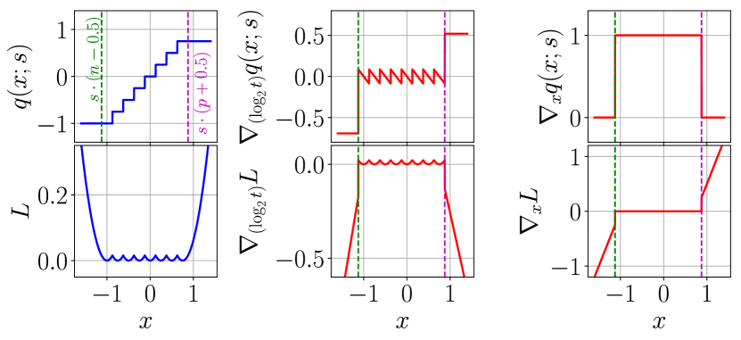
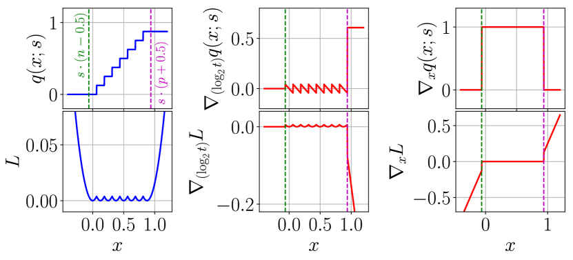
Figure 1 shows the forward and backward pass transfer curves for our quantizer. As noted, the exact clipping thresholds of in the real domain are and .
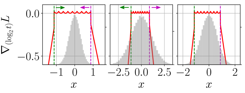
Role of threshold gradients: As seen from the plots of vs. in Figure 2, threshold gradients are positive for within clipping thresholds and negative otherwise. When most of the input distribution444Gaussian in this example, but the analysis holds in general. falls within , the cumulative threshold gradient is positive causing to decrease555From the update rule where is the learning rate.. In other words, the limits get pulled inward in favor of larger precision. Similarly, when most of the input distribution falls outside , the cumulative threshold gradient is negative, increases, and the limits get pushed outward in favor of larger dynamic range. This technique is naturally robust to distributions with long tails or outliers, by achieving range-precision trade-off through gradient-based optimization.
Role of Input Gradients: Using a similar analysis as for threshold gradients, we see that the input gradients are non-zero for values of that fall outside , biased to keep them from getting clipped. This encourages the weight and activation distributions to be tighter.
To summarize, threshold gradients help train optimal thresholds for clipping weights and activations, whereas input gradients nudge the weights and activations to tighter bounds. By simultaneously training clipping thresholds and weights of the quantized network through backpropagation, we adopt joint (mutual) optimization over a global loss.
3.5 Comparison to Clipped Threshold Gradients
In contrast, certain quantizer implementations define threshold gradients by simply clipping the upstream gradients at the saturation thresholds. For example TensorFlow’s FakeQuant (used for QAT) defines gradients with respect to min/max thresholds as a clip function.
In the forward pass, FakeQuant operation TensorFlow (2016a) is mathematically equivalent to our formulation (except with zero-point), defined as:
| (11) |
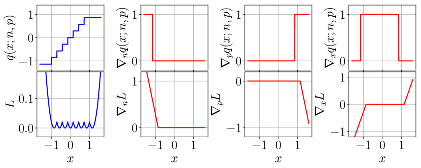
However, in the backward pass they treat the round function in (11) to be identity, reducing (11) to a clip function with clipped gradients. That is, gradients with respect to thresholds are trivially clipped to zero for within , as seen in FakeQuant’s transfer curves in Figure 3 and its kernel definition TensorFlow (2016b). As a result, the overall gradients only push the limits outward, training to the min/max of the input distributions and strictly favoring range over precision. We believe this behavior can be corrected to allow effective range-precision trade-off, as seen in Figure 2 with the toy model, by carefully using the STE such that , but in the backward pass. While the actual loss landscape is non-trivial, we empirically observe similar qualitative behavior to our toy model, in Section 5.3.
Another popular clipping threshold method (applicable to ReLU activations) is PACT, which has similar behavior to TensorFlow’s FakeQuant. As seen in (1), the gradient with respect to clipping threshold takes a value of either 0 or 1 depending on whether the quantizer input lies to the left or right of . This results in a tendency of to train to the max limits of the distribution of . To combat this tendency, a regularizer on the magnitude of is applied to the loss function. However, this requires an additional parameter to be tuned manually and has no awareness for the loss landscape or the quantization bitwidth.
4 Framework for TQT
We released Graffitist666Available at github.com/Xilinx/graffitist., an end-to-end software stack built on top of TensorFlow, to quantize and retrain deep neural networks (DNNs) using TQT for accurate and efficient inference on fixed-point hardware. Fundamentally, Graffitist is a flexible and scalable framework to process low-level graph descriptions of DNNs, comprising of a (growing) library of transforms to implement various neural net optimizations. Each graph transform consists of unique pattern matching and manipulation algorithms that when run sequentially produce an optimized output graph. It is still in experimental stages as we continue to add support for more operation types, layer topologies, network styles, graph optimizations, and compression techniques. Graffitist stands on the shoulders of giants and the interface is inspired in part by earlier tools from TensorFlow tf-graphtransformtool; TensorFlow (2017a).
4.1 Graph Optimizations
Graffitist applies several optimizations to the input graph prior to quantization. For example, folding batch normalization layers into preceding convolutional or fully connected or depthwise convolutional layers’ weights. We adopt the following best practices from Jacob et al. (2017); Krishnamoorthi (2018); TensorFlow (2017a): (a) ensure folded batch norms in training and inference graphs are mathematically equivalent (i.e., distributions seen during training match those during inference); (b) apply batch norm corrections for switching between batch and moving average statistics to reduce jitter in training folded weights due to noisy batch updates; (c) freeze batch norm moving mean and variance updates post convergence for improved accuracy. Other optimizations include collapsing concat-of-concat layers into single concat, splicing identity nodes not involved in control edges, transforming average pool layers into depthwise conv layers with reciprocal777Reciprocal being where is the kernel size. multiplier as weights, and explicitly merging input scales for scale preserving ops such as concat, bias-add, eltwise-add, and maximum (for leaky relu).
4.2 Quantization Modes
Graffitist allows for quantization in either static or retrain modes.
Static Mode. Quantization thresholds (hence scale factors) are determined based on statistics of weights and activations derived from a calibration dataset. Specifically, weight thresholds (per-tensor) are set to the maximum absolute value (Table 2), and activation thresholds (per-tensor) are chosen such as to minimize the symmetric Kullback-Leibler-J distance D’Alberto & Dasdan (2009) for each quantization layer locally. This is done in a strictly topological order to ensure inputs to a layer are quantized (and fixed) prior to quantizing the current layer. The entire optimization and calibration process is automated and only requires a single API call to Graffitist.
Retrain Mode. Quantization thresholds and weights are simultaneously trained on a global loss. Recovery is achieved within 5 epochs of TQT retraining. This requires two separate API calls to Graffitist - first to generate a quantized training graph that can be trained with native TensorFlow on GPU, and second to generate an equivalent quantized inference graph that accurately models the target fixed-point implementation. The benefit of a hardware-accurate inference graph is twofold: (i) much before deployment, one can quickly validate the inference accuracy of the quantized network using CPU/GPU, and (ii) scale factors and quantized weights from TQT can be ported directly onto the target of choice. On tests across several networks, we found that our inference graphs run on the CPU were bit-accurate to our fixed-point implementation on the FPGA.
4.3 Layer Precisions
While Graffitist supports configurable bit-widths for weights and activations, for the scope of this paper we use two modes: INT8 with 8/8 (W/A) and INT4 with 4/8 (W/A). The choice of 4/8 as opposed to 4/4 is primarily guided by the availability of 4x8 multipliers; even in the absence of this, the INT4 mode still allows for 50% weight compression (double packing weights per byte) and reduced memory footprint for fetching weights. The internal precisions for different layer topologies are defined below. Quantization layers marked as indicate that their scale-factors are explicitly merged / shared. To avoid double quantization, input tensors are assumed to be already quantized by the previous layer, with the exception of the primary input (placeholder) which is explicitly quantized.
-
•
Compute layers (e.g., conv, matmul, depthwise conv) are quantized as:
where is the input tensor, is the weight tensor, and is the bias tensor. If followed by a ReLU or ReLU6 activation function, the last stage is delayed to until after ReLU/ReLU6, and uses unsigned datatype to utilize the extra sign bit.
-
•
Eltwise-add layer is quantized as:
where and are the input tensors. Similar to the compute layer case, the last stage is delayed and uses unsigned datatype if followed by ReLU/ReLU6.
-
•
Leaky ReLU is quantized as:
where is the input tensor, and is the slope of activation function for negative inputs. The last stage on the previous compute layer is skipped when it is followed by Leaky ReLU. Instead a stage is used to retain high internal precision for the -multiply op.
-
•
Average pool is quantized as:
where is the input tensor, and is the reciprocal.
-
•
Concat is not quantized because the input scales are merged explicitly, and hence it is lossless:
where , , and are input tensors.
4.4 Fused Kernel Implementation
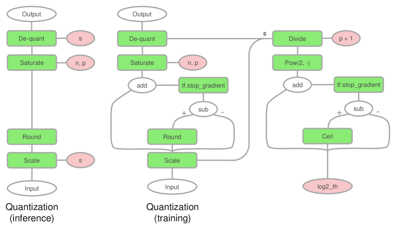
The quantization layer defined in (4) and (6) may be trivially implemented using native TensorFlow ops and tf.stop_gradient as depicted in Figure 4. However this low-level implementation has a large memory footprint during training due to the need for storing intermediate tensors for gradient computation in the backward pass. This impacts the maximum batch size that can fit on a single GPU. To overcome this, Graffitist is packaged with fused quantization kernels that are pre-compiled for CPU/GPU. The fused implementation is efficient, helps avoid memory overhead and allows training using larger batch sizes compared to the native implementation.
5 Experiments
We evaluate TQT on variants of five classes of CNNs trained and validated on ImageNet (ILSVRC14) classification dataset Russakovsky et al. (2015). The networks include VGG {16, 19} Simonyan & Zisserman (2014), Inception v{1, 2, 3, 4} Szegedy et al. (2014); Ioffe & Szegedy (2015); Szegedy et al. (2015; 2016), ResNet v1 {50, 101, 152} He et al. (2015), MobileNet v{1, 2} 1.0 224 Howard et al. (2017); Sandler et al. (2018), and DarkNet 19 Redmon & Farhadi (2016). We obtained the models, pre-trained weights (FP32) and pre-processing for each of these networks from the TF-Slim model zoo TensorFlow (2017b) except for DarkNet 19 which was converted to TensorFlow using DW2TF Hao & Jain (2018).
We are interested in a scalable and production-ready approach to INT8/INT4 quantization that maps well on generic fixed-point hardware. While our simplifying constraints (from Section 3.1) may not be ideal for lower bit-widths, the fundamentals of TQT are more generally applicable even without these constraints. To limit the scope of this paper to the least-common-denominator fixed-point quantization, we do not make comparisons with other state-of-the-art low-bitwidth quantization schemes. Instead we draw comparisons of TQT (wt+th) retraining to static quantization and wt-only retraining. We can derive many interesting insights from this analysis.
5.1 Threshold Initializations
| Mode | Threshold Initialization | ||
|---|---|---|---|
| weights | activations | ||
| Static | MAX | KL-J | |
| \hdashlineRetrain | wt | MAX | KL-J |
| wt,th | 3SD | KL-J | |
Calibration sets are prepared for each network using a batch of 50 unlabeled images, randomly sampled from the validation set, with applied pre-processing. This is used for initializing the thresholds in both static and retrain modes. When thresholds are not trained, they are initialized to MAX for weights, and KL-J distance calibrated for activations. However when training thresholds, we find it useful to initialize the weight thresholds based on standard deviations or percentile of the weight distribution rather than MAX. Table 2 summarizes the threshold initialization scheme we used for all our experiments.
5.2 Implementation Details
Before exporting the models to TensorFlow protocol buffers (.pb) for Graffitist to absorb, we make the following synthetic modifications: (i) replace tf.reduce_mean with tf.nn.avg_pool (if any), (ii) remove auxiliary logit layers (if any), and (iii) remove dropouts (if any). Additionally, we disable data-augmentation (e.g., random flip / crop) during retraining. These modifications are done keeping in mind that TQT focuses primarily on learning thresholds through backpropagation, while allowing previously trained weights to be fine-tuned using a relatively small learning rate. As expected, most of the recovery is achieved within a fraction of an epoch due to thresholds converging, and the rest of it (up to 5 epochs) is just weights adjusting to the new thresholds. Because the overall training steps required with TQT are so few compared to from-scratch training, and that pre-trained weight distributions are not allowed to wildly change (overfit), we find it best to disable data-augmentation and dropout regularization.
Based on the stability analysis and hyperparameter recommendations in Appendix B.2 and B.3, we use the Adam optimizer with parameters and for training thresholds and weights in all our experiments. The initial learning rate is set to for thresholds and for weights. Learning rates are decayed exponentially (with staircase enabled) by a factor of every steps for weights and by a factor of every steps for thresholds, where is the batch size. We use a batch size of 24 for all networks except for ResNet v1 152 and Inception v4 for which a batch of 16 is used. Softmax cross-entropy loss is used to compute quantization threshold gradients and this loss, together with weight regularization (if any), are used to compute weight gradients. Batch norm moving means and variances are frozen after epoch.
In Appendix B.3, we discussed the post-convergence oscillations of thresholds around the critical integer threshold due to our power-of-2 scaling constraint. When thresholds cross this integer level, it can change the distributions of downstream activations, requiring weights and thresholds of the following layers to adapt to it. To minimize this effect, we incrementally freeze thresholds starting at steps, once every 50 steps in the order of increasing absolute gradient magnitude, if they are on the correct side of (determined using an EMA). This is automatically handled by the training scripts packaged with Graffitist.
5.3 Results
| Mode | Precision | Bit-width | Accuracy (%) | Epochs | ||
|---|---|---|---|---|---|---|
| (W/A) | top-1 | top-5 | ||||
| VGG 16 | ||||||
| \hdashline | FP32 | 32/32 | 70.9 | 89.8 | ||
| Static | INT8 | 8/8 | 70.4 | 89.7 | ||
| \hdashline Retrain | wt | FP32 | 32/32 | 71.9 | 90.5 | 1.0 |
| wt | INT8 | 8/8 | 71.8 | 90.5 | 1.0 | |
| wt,th | INT8 | 8/8 | 71.7 | 90.4 | 0.9 | |
| wt,th | INT4 | 4/8 | 71.5 | 90.3 | 4.0 | |
| VGG 19 | ||||||
| \hdashline | FP32 | 32/32 | 71.0 | 89.8 | ||
| Static | INT8 | 8/8 | 70.4 | 89.7 | ||
| \hdashline Retrain | wt | FP32 | 32/32 | 71.8 | 90.4 | 1.0 |
| wt | INT8 | 8/8 | 71.7 | 90.4 | 1.0 | |
| wt,th | INT8 | 8/8 | 71.7 | 90.4 | 1.0 | |
| wt,th | INT4 | 4/8 | 71.2 | 90.1 | 2.0 | |
| Inception v1 | ||||||
| \hdashline | FP32 | 32/32 | 69.8 | 89.6 | ||
| Static | INT8 | 8/8 | 68.6 | 88.9 | ||
| \hdashline Retrain | wt | FP32 | 32/32 | 70.3 | 90.0 | 2.8 |
| wt | INT8 | 8/8 | 70.6 | 90.3 | 3.5 | |
| wt,th | INT8 | 8/8 | 70.7 | 90.2 | 2.4 | |
| wt,th | INT4 | 4/8 | 67.2 | 88.2 | 4.0 | |
| Inception v2 | ||||||
| \hdashline | FP32 | 32/32 | 74.0 | 91.8 | ||
| Static | INT8 | 8/8 | 73.1 | 91.3 | ||
| \hdashline Retrain | wt | FP32 | 32/32 | 74.3 | 92.2 | 3.3 |
| wt | INT8 | 8/8 | 74.4 | 92.3 | 4.7 | |
| wt,th | INT8 | 8/8 | 74.4 | 92.4 | 2.5 | |
| wt,th | INT4 | 4/8 | 71.9 | 90.8 | 4.8 | |
| Inception v3 | ||||||
| \hdashline | FP32 | 32/32 | 78.0 | 93.9 | ||
| Static | INT8 | 8/8 | 76.8 | 93.3 | ||
| \hdashline Retrain | wt | FP32 | 32/32 | 78.3 | 94.2 | 2.1 |
| wt | INT8 | 8/8 | 78.2 | 94.1 | 2.0 | |
| wt,th | INT8 | 8/8 | 78.3 | 94.3 | 1.2 | |
| wt,th | INT4 | 4/8 | 76.4 | 93.1 | 4.4 | |
| Inception v4 | ||||||
| \hdashline | FP32 | 32/32 | 80.2 | 95.2 | ||
| Static | INT8 | 8/8 | 79.4 | 94.6 | ||
| \hdashline Retrain | wt | FP32 | 32/32 | 80.2 | 95.2 | 0.0 |
| wt | INT8 | 8/8 | 80.1 | 95.3 | 1.7 | |
| wt,th | INT8 | 8/8 | 80.1 | 95.2 | 1.5 | |
| wt,th | INT4 | 4/8 | 78.9 | 94.7 | 4.2 | |
| Mode | Precision | Bit-width | Accuracy (%) | Epochs | ||
|---|---|---|---|---|---|---|
| (W/A) | top-1 | top-5 | ||||
| MobileNet v1 1.0 224 | ||||||
| \hdashline | FP32 | 32/32 | 71.0 | 90.0 | ||
| Static | INT8 | 8/8 | 0.6 | 3.6 | ||
| \hdashline Retrain | wt | FP32 | 32/32 | 71.1 | 90.0 | 3.4 |
| wt | INT8 | 8/8 | 67.0 | 87.9 | 4.6 | |
| wt,th | INT8 | 8/8 | 71.1 | 90.0 | 2.1 | |
| wt,th | INT4 | 4/8 | – | – | ||
| MobileNet v2 1.0 224 | ||||||
| \hdashline | FP32 | 32/32 | 70.1 | 89.5 | ||
| Static | INT8 | 8/8 | 0.3 | 1.2 | ||
| \hdashline Retrain | wt | FP32 | 32/32 | 71.7 | 90.7 | 3.2 |
| wt | INT8 | 8/8 | 68.2 | 89.0 | 2.7 | |
| wt,th | INT8 | 8/8 | 71.8 | 90.6 | 2.2 | |
| wt,th | INT4 | 4/8 | – | – | ||
| DarkNet 19 | ||||||
| \hdashline | FP32 | 32/32 | 73.0 | 91.4 | ||
| Static | INT8 | 8/8 | 68.7 | 89.7 | ||
| \hdashline Retrain | wt | FP32 | 32/32 | 74.4 | 92.3 | 3.1 |
| wt | INT8 | 8/8 | 72.9 | 91.6 | 3.8 | |
| wt,th | INT8 | 8/8 | 74.5 | 92.3 | 1.8 | |
| wt,th | INT4 | 4/8 | 73.2 | 91.6 | 2.8 | |
| ResNet v1 50 | ||||||
| \hdashline | FP32 | 32/32 | 75.2 | 92.2 | ||
| Static | INT8 | 8/8 | 74.3 | 91.7 | ||
| \hdashline Retrain | wt | FP32 | 32/32 | 75.4 | 92.5 | 3.7 |
| wt | INT8 | 8/8 | 75.3 | 92.3 | 1.0 | |
| wt,th | INT8 | 8/8 | 75.4 | 92.3 | 1.9 | |
| wt,th | INT4 | 4/8 | 74.4 | 91.7 | 2.0 | |
| ResNet v1 101 | ||||||
| \hdashline | FP32 | 32/32 | 76.4 | 92.9 | ||
| Static | INT8 | 8/8 | 74.8 | 92.0 | ||
| \hdashline Retrain | wt | FP32 | 32/32 | 76.6 | 93.2 | 1.2 |
| wt | INT8 | 8/8 | 76.3 | 93.0 | 1.0 | |
| wt,th | INT8 | 8/8 | 76.4 | 93.1 | 0.9 | |
| wt,th | INT4 | 4/8 | 75.7 | 92.5 | 2.0 | |
| ResNet v1 152 | ||||||
| \hdashline | FP32 | 32/32 | 76.8 | 93.2 | ||
| Static | INT8 | 8/8 | 76.2 | 93.0 | ||
| \hdashline Retrain | wt | FP32 | 32/32 | 76.8 | 93.3 | 1.0 |
| wt | INT8 | 8/8 | 76.7 | 93.3 | 1.5 | |
| wt,th | INT8 | 8/8 | 76.7 | 93.3 | 1.4 | |
| wt,th | INT4 | 4/8 | 76.0 | 93.0 | 1.9 | |
Table 3 reports the single-crop ImageNet validation accuracy for 12 networks. Default image sizes are used: for Inception v{3, 4}, for Darknet 19 and for all other networks. Standard pre-processing for each network is applied to center crop, resize, and normalize the input data. The different trials include pre-trained FP32 baseline, static INT8 run, and 4 retrain runs - FP32 wt-only, INT8 wt-only, INT8 wt+th and INT4 wt+th. Here, INT8 is 8/8 (W/A) and INT4 is 4/8 (W/A). FP32 baseline numbers are reported as validated on our end. For an unbiased comparison, we train the FP32 weights using the same procedure (optimizers, learning rates, decay, BN freeze etc.) as with our quantized weight retraining. This FP32 wt-only retraining serves as a fair baseline to our INT8 and INT4 retrain results. That said, we do not use the retrained FP32 weights to initialize any of our INT8/INT4 retraining runs, and they always start from pre-trained FP32 weights. This is done to keep the overhead of retraining to a minimum.
6 Discussion
The validation accuracy and epoch count corresponding to the best checkpoint are noted in Table 3. As we see, all the networks converge within 5 epochs. Variance on the reported accuracy stems from a few sources (in decreasing order): (a) best rather than mean validation (our findings in Appendix D suggest this variance is within 0.2%), (b) non-determinism due to inexact floating point math (empirically within 0.1%), (c) round to one decimal (bound to 0.05%). Keeping these variance bounds on accuracy in mind, we can draw interesting insights into the benefits of TQT.
6.1 Insights from TQT
Our experiments demonstrate floating-point accuracy for 8-bit quantization and near-floating-point accuracy for 4-bit quantization for most networks. We see that static quantization incurs a higher loss than retrained methods. This is expected because (a) weights are not trained to adapt to the quantized network, and (b) quantization thresholds are picked using local statistics instead of being optimized on a global loss. For networks that are easier to quantize to INT8 (e.g., VGGs, Inceptions, ResNets), we find that retraining weights alone while fixing thresholds to their pre-calibrated values (based on Table 2) is sufficient. In such cases, TQT (wt+th) retraining shows no added benefit. However, for networks known to be difficult to quantize (e.g., MobileNets, DarkNets), TQT (wt+th) retraining yields up to higher top-1 accuracy compared to wt-only training for INT8, and can match FP32 accuracy even with per-tensor, uniform symmetric, power-of-2 scaling constraints. This demonstrates the range-precision trade-off through trained thresholds in action. For lower precisions such as INT4, we find that wt-only training does not recover, and so TQT (wt+th) retraining is necessary. The INT4 accuracy falls short of FP32, and we believe this maybe due to (a) our quantization constraints in Section 3.1, and (b) the first/last layers not retaining full precision888We quantize first/last layers to a minimum of INT8, so that they can be mapped on the same fixed-point hardware used for other layers..
6.2 MobileNet Comparisons
For more difficult networks such as MobileNets, it is well known that symmetric, per-tensor quantization done post-training or through calibrate-only methods is detrimental Krishnamoorthi (2018); Goncharenko et al. (2018). We believe this is true, in particular due to the use of depthwise convolutions with irregular weight distributions and widely varying ranges between channels. With wt-only retraining we are only able to recover to within of floating-point accuracy. However, with TQT (wt+th) retraining, our results for 8-bit are the highest we have seen using symmetric, power-of-2 scaled, per-tensor quantization, even matching floating-point accuracy with no loss. We draw a few comparisons with Google’s QAT results for MobileNets in Table 1 and observe that we incur no loss with INT8 quantization even with stricter constraints. We believe this is due to the fact that our threshold gradient formulation is in fact able to balance range-precision effectively.
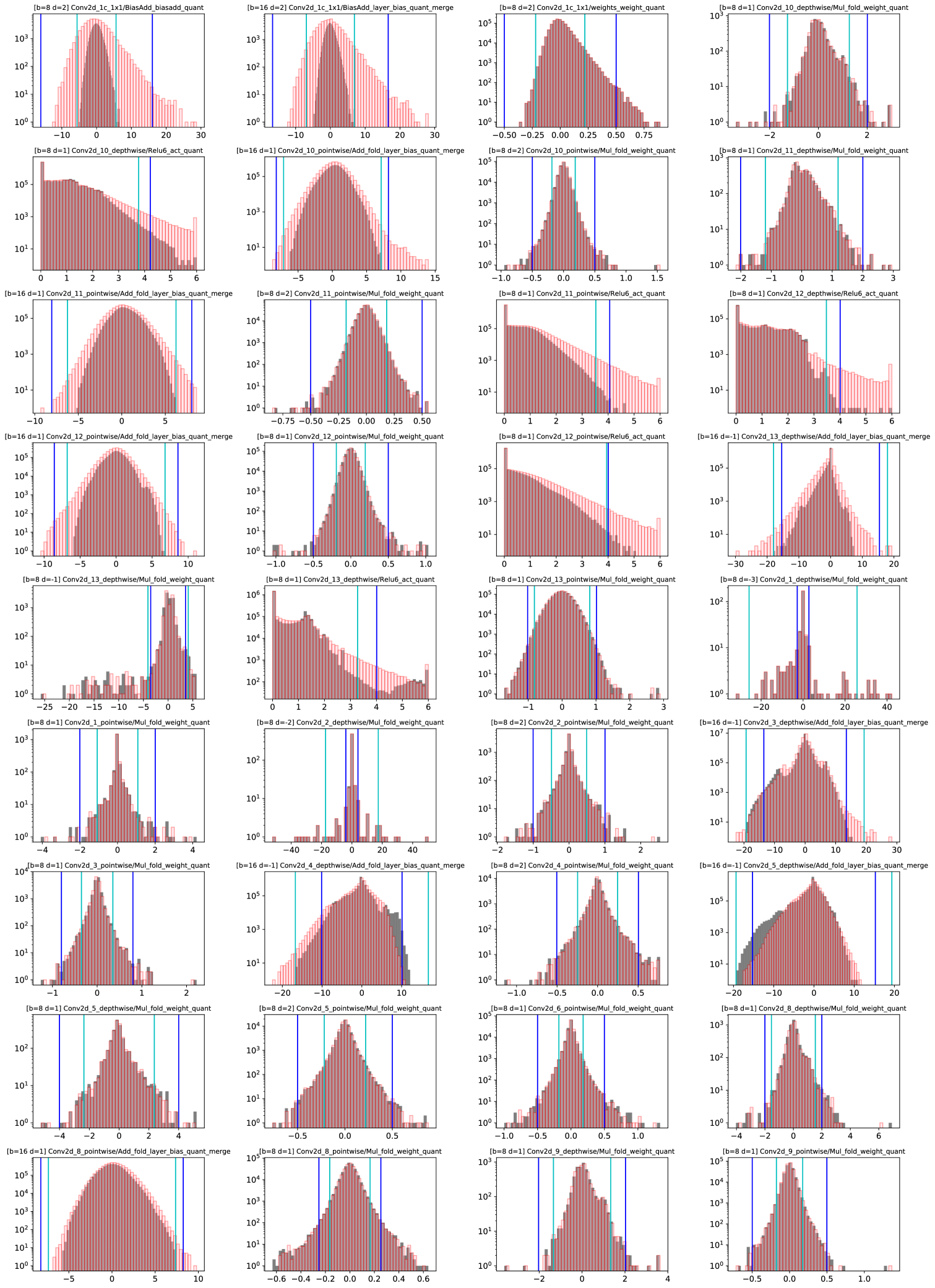
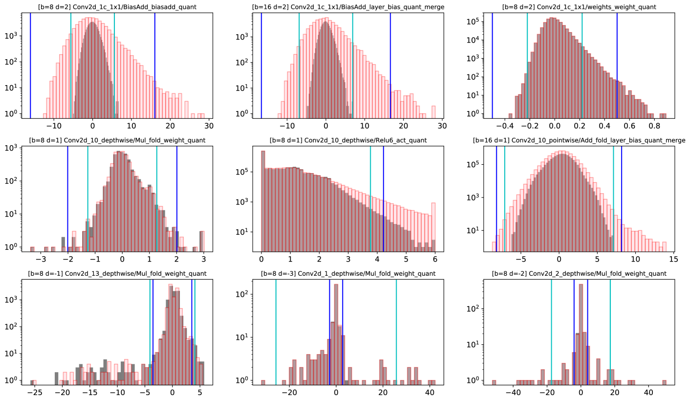
In Figure 5 we analyze the retrained distributions for a few quantized layers in MobileNet v1, highlighting the importance of range-precision trade-off. As seen with the depthwise convolutional layers’ weights, the trained thresholds move-in from their initialized values by up to 3 integer bins in the log-domain, favoring precision over dynamic range. For some other layers, the thresholds move-out from their initialized values, favoring range over precision. For more such layers with non-zero threshold deviations, see Figure 10 in Appendix.
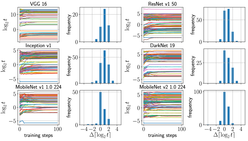
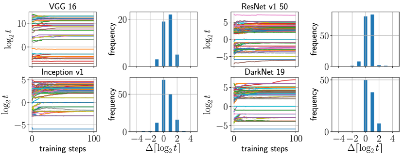
Figure 6 shows a histogram of deviations of trained thresholds for different networks under 8-bit and 4-bit quantized retraining. We find that larger positive deviations are seen in the 8-bit case compared to the 4-bit case. This intuitively makes sense as the method decides to favor range with more bits of precision, but cuts back on range when only few bits of precision are available.
7 Conclusion
In Section 3, we proposed a general method for training quantization thresholds (TQT), amenable to most generic fixed-point hardware by constraining our method to uniform, symmetric, power-of-2 scaled, per-tensor quantization. We showed that our quantizer’s gradient formulation allowed a unique range-precision trade-off, essential for high-accuracy quantized networks. We demonstrated a robust, fast convergence training scheme for TQT utilizing log-domain threshold training with an adaptive optimizer. In Section 4, we presented Graffitist, a framework for automatic quantization and retraining of TensorFlow graphs with our methods. In Section 5, we empirically validated our methods on a suite of standard CNNs trained on ImageNet. Finally, in Sections 6, we provided insightful discussions on TQT and state-of-the-art results for 8-bit MobileNet quantization.
Our work and results demonstrate the effectiveness of our techniques for high accuracy quantization of neural networks for fixed-point inference. While our work covers a major use case for quantization, there are many other quantization flavors we could explore in future work. For example, it would be useful to see how well the techniques we designed for strict power-of-2 scaling generalize to non power-of-2 scale-factors. Some additional relaxations of our constraints we could explore include per-channel rather than per-tensor quantization, which could potentially allow for more aggressive bitwidths on difficult networks like MobileNets, and non-symmetric or even non-uniform quantization schemes, where threshold training via backpropagation and gradient descent has been tried with mild success. We would not be surprised to see our methods and analysis techniques have broader applicability for more general classes of quantizers and problems beyond ImageNet.
References
- Baskin et al. (2018) Baskin, C., Liss, N., Chai, Y., Zheltonozhskii, E., Schwartz, E., Giryes, R., Mendelson, A., and Bronstein, A. M. Nice: Noise injection and clamping estimation for neural network quantization. arXiv preprint arXiv:1810.00162, 2018.
- Bengio et al. (2013) Bengio, Y., Léonard, N., and Courville, A. Estimating or propagating gradients through stochastic neurons for conditional computation. arXiv preprint arXiv:1308.3432, 2013.
- Cai et al. (2017) Cai, Z., He, X., Sun, J., and Vasconcelos, N. Deep learning with low precision by half-wave gaussian quantization. arXiv preprint arXiv:1702.00953, 2017.
- Choi et al. (2018) Choi, J., Wang, Z., Venkataramani, S., Chuang, P. I.-J., Srinivasan, V., and Gopalakrishnan, K. Pact: Parameterized clipping activation for quantized neural networks. arXiv preprint arXiv:1805.06085, 2018.
- Courbariaux et al. (2016) Courbariaux, M., Hubara, I., Soudry, D., El-Yaniv, R., and Bengio, Y. Binarized neural networks: Training deep neural networks with weights and activations constrained to+ 1 or-1. arXiv preprint arXiv:1602.02830, 2016.
- D’Alberto & Dasdan (2009) D’Alberto, P. and Dasdan, A. Non-parametric information-theoretic measures of one-dimensional distribution functions from continuous time series. In Proceedings of the 2009 SIAM International Conference on Data Mining, pp. 685–696. SIAM, 2009.
- Esser et al. (2019) Esser, S. K., McKinstry, J. L., Bablani, D., Appuswamy, R., and Modha, D. S. Learned step size quantization. arXiv preprint arXiv:1902.08153, 2019.
- Goncharenko et al. (2018) Goncharenko, A., Denisov, A., Alyamkin, S., and Terentev, E. Fast adjustable threshold for uniform neural network quantization. arXiv preprint arXiv:1812.07872, 2018.
- Hao & Jain (2018) Hao, Y. and Jain, S. R. Darknet to tensorflow (DW2TF). https://github.com/jinyu121/DW2TF/releases/tag/v1.2, 2018.
- He et al. (2015) He, K., Zhang, X., Ren, S., and Sun, J. Deep residual learning for image recognition. arXiv preprint arXiv:1512.03385, 2015.
- Hinton et al. (2012) Hinton, G., Srivastava, N., and Swersky, K. Lecture 6a overview of mini-batch gradient descent (2012). Coursera Lecture slides https://class. coursera. org/neuralnets-2012-001/lecture, 2012.
- Howard et al. (2017) Howard, A. G., Zhu, M., Chen, B., Kalenichenko, D., Wang, W., Weyand, T., Andreetto, M., and Adam, H. Mobilenets: Efficient convolutional neural networks for mobile vision applications. arXiv preprint arXiv:1704.04861, 2017.
- Ioffe & Szegedy (2015) Ioffe, S. and Szegedy, C. Batch normalization: Accelerating deep network training by reducing internal covariate shift. arXiv preprint arXiv:1502.03167, 2015.
- Jacob et al. (2017) Jacob, B., Kligys, S., Chen, B., Zhu, M., Tang, M., Howard, A., Adam, H., and Kalenichenko, D. Quantization and training of neural networks for efficient integer-arithmetic-only inference. arXiv preprint arXiv:1712.05877, 2017.
- Jacob et al. (2016a) Jacob, B. et al. Gemmlowp: Efficient handling of offsets. https://github.com/google/gemmlowp/blob/master/doc/low-precision.md#efficient-handling-of-offsets, 2016a.
- Jacob et al. (2016b) Jacob, B. et al. Gemmlowp: Building a quantization paradigm from first principles. https://github.com/google/gemmlowp/blob/master/doc/quantization.md, 2016b.
- Jung et al. (2018) Jung, S., Son, C., Lee, S., Son, J., Kwak, Y., Han, J.-J., Hwang, S. J., and Choi, C. Learning to quantize deep networks by optimizing quantization intervals with task loss. arXiv preprint arXiv:1808.05779, 2018.
- Kingma & Ba (2014) Kingma, D. P. and Ba, J. Adam: A method for stochastic optimization. arXiv preprint arXiv:1412.6980, 2014.
- Krishnamoorthi (2018) Krishnamoorthi, R. Quantizing deep convolutional networks for efficient inference: A whitepaper. arXiv preprint arXiv:1806.08342, 2018.
- Li et al. (2016) Li, F., Zhang, B., and Liu, B. Ternary weight networks. arXiv preprint arXiv:1605.04711, 2016.
- McKinstry et al. (2018) McKinstry, J. L., Esser, S. K., Appuswamy, R., Bablani, D., Arthur, J. V., Yildiz, I. B., and Modha, D. S. Discovering low-precision networks close to full-precision networks for efficient embedded inference. arXiv preprint arXiv:1809.04191, 2018.
- Migacz (2017) Migacz, S. 8-bit inference with tensorrt. In GPU Technology Conference, 2017.
- Mishra et al. (2017) Mishra, A., Nurvitadhi, E., Cook, J. J., and Marr, D. Wrpn: wide reduced-precision networks. arXiv preprint arXiv:1709.01134, 2017.
- Rastegari et al. (2016) Rastegari, M., Ordonez, V., Redmon, J., and Farhadi, A. Xnor-net: Imagenet classification using binary convolutional neural networks. arXiv preprint arXiv:1603.05279, 2016.
- Redmon & Farhadi (2016) Redmon, J. and Farhadi, A. Yolo9000: Better, faster, stronger. arXiv preprint arXiv:1612.08242, 2016.
- Russakovsky et al. (2015) Russakovsky, O., Deng, J., Su, H., Krause, J., Satheesh, S., Ma, S., Huang, Z., Karpathy, A., Khosla, A., Bernstein, M., Berg, A. C., and Fei-Fei, L. ImageNet Large Scale Visual Recognition Challenge. International Journal of Computer Vision (IJCV), 115(3):211–252, 2015. doi: 10.1007/s11263-015-0816-y.
- Sandler et al. (2018) Sandler, M., Howard, A., Zhu, M., Zhmoginov, A., and Chen, L.-C. Mobilenetv2: Inverted residuals and linear bottlenecks. arXiv preprint arXiv:1801.04381, 2018.
- Simonyan & Zisserman (2014) Simonyan, K. and Zisserman, A. Very deep convolutional networks for large-scale image recognition. arXiv preprint arXiv:1409.1556, 2014.
- Szegedy et al. (2014) Szegedy, C., Liu, W., Jia, Y., Sermanet, P., Reed, S., Anguelov, D., Erhan, D., Vanhoucke, V., and Rabinovich, A. Going deeper with convolutions. arXiv preprint arXiv:1409.4842, 2014.
- Szegedy et al. (2015) Szegedy, C., Vanhoucke, V., Ioffe, S., Shlens, J., and Wojna, Z. Rethinking the inception architecture for computer vision. arXiv preprint arXiv:1512.00567, 2015.
- Szegedy et al. (2016) Szegedy, C., Ioffe, S., Vanhoucke, V., and Alemi, A. Inception-v4, inception-resnet and the impact of residual connections on learning. arXiv preprint arXiv:1602.07261, 2016.
- TensorFlow (2016a) TensorFlow. FakeQuant API. https://www.tensorflow.org/versions/r1.13/api_docs/python/tf/quantization/fake_quant_with_min_max_vars, 2016a.
- TensorFlow (2016b) TensorFlow. FakeQuant threshold gradients. https://github.com/tensorflow/tensorflow/blob/v1.13.1/tensorflow/core/kernels/fake_quant_ops_functor.h#L179-L187, 2016b.
- TensorFlow (2017a) TensorFlow. Quantization-aware training. https://github.com/tensorflow/tensorflow/blob/v1.13.1/tensorflow/contrib/quantize/README.md, 2017a.
- TensorFlow (2017b) TensorFlow. Tf-slim pre-trained models. https://github.com/tensorflow/models/blob/v1.13.0/research/slim/README.md#pre-trained-models, 2017b.
- Zhang et al. (2018) Zhang, D., Yang, J., Ye, D., and Hua, G. Lq-nets: Learned quantization for highly accurate and compact deep neural networks. arXiv preprint arXiv:1807.10029, 2018.
- Zhou et al. (2016) Zhou, S., Wu, Y., Ni, Z., Zhou, X., Wen, H., and Zou, Y. Dorefa-net: Training low bitwidth convolutional neural networks with low bitwidth gradients. arXiv preprint arXiv:1606.06160, 2016.
- Zhu et al. (2016) Zhu, C., Han, S., Mao, H., and Dally, W. J. Trained ternary quantization. arXiv preprint arXiv:1612.01064, 2016.
Appendix A Cost of Affine Quantizer
A.1 Cross-terms due to zero-points
Consider two real numbers and and their product . Using the affine mapping from (2) to represent this, we get:
| (12) |
which can be expressed as
| (13) |
The cross-terms in (13) add complexity and often require special handling to remain efficient. While the added cost can be amortized over several accumulations of a matrix multiplication or convolution operation, it would still require optimizations999Some of which are covered in Jacob et al. (2016a; 2017); Krishnamoorthi (2018)., both algorithmic and kernel-level.
By eliminating zero-points, the cross-terms vanish and the operation simplifies to:
| (14) |
A.2 Real-valued scale-factors
With positive real scale-factors, the constant multiplier in (14), empirically found to be in the interval (0, 1) Jacob et al. (2017), can be expressed in the normalized form where is a non-negative integer and is in the interval [0.5, 1). In other words, the accumulator (storing ) needs to be scaled by a fixed-point multiplier that approximates and right-shifted by bits (with round-to-nearest):
| (15) |
However, by constraining scale-factors to strict power-of-2, the scaling operation reduces to a rather simple bit-shift (with round-to-nearest):
| (16) |
Appendix B Log Threshold Training
Initially, it may seem that with the definition of a gradient with respect to the raw threshold, backpropagation and gradient descent could be immediately used to train it. However, just as training weights in a vanilla neural network requires care in the choice of optimizer and learning rate, here too care must be taken to ensure training stability and convergence. There are three main properties we would like our training procedure to satisfy: numerical stability, scale invariance, and convergence. We discuss each of these issues and the engineering tweaks used to solve them here.
B.1 Numerical Stability
One obvious problem with training raw thresholds is that gradient updates could potentially bump a threshold to a negative value, causing and therefore scale-factor to diverge. If this happens even once, the network as a whole will break. An easy solution is to train as opposed to itself, since its domain is . Using log thresholds is convenient because it already appears in the expression for . However, the most important benefit is described in Section B.2, where the log representation makes ensuring scale invariance very easy.
B.2 Scale Invariance
For a given input distribution we prefer that the threshold gradients have similar magnitudes regardless of the position of the threshold itself. This threshold scale invariance is useful for making sure training is not too slow when the thresholds are far from their optimal values. Similarly, the properties of our threshold gradients should not depend on the scale of the input distribution. This input scale invariance is important because it ensures that quantized training behaves the same way for the different weights and activations in the network, even if the variance of their distributions vary over many orders of magnitude.
Unfortunately, neither of these scale invariances hold. Far from improving, Figure 7 shows that in moving from raw threshold training (left) to log threshold training (middle), both scale invariance properties of the threshold gradients actually degrade.

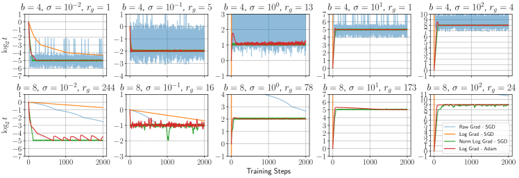
Threshold scale invariance: Updates to the log threshold would be threshold scale invariant if the gradients on both sides of the negative-to-positive jump were flat, as seen in the right plot of Figure 7. However, this is not the case for log threshold gradients (center plot of Figure 7). On the left-of-jump side, as decreases, gradients of (hence updates to) get exponentially smaller, meaning it will converge very slowly to lower optimal values (see the log grad SGD case in the left plots of Figure 8). Similarly, on the right-of-jump side, as increases, updates to increase exponentially, meaning it will converge very quickly and possibly unstably to higher optimal values (see the log grad SGD case in the right plots of Figure 8). In the raw threshold domain, we would like gradients of (hence updates to) to scale proportional to . This is also not the case for the left-of-jump side of raw threshold gradients (left plot of Figure 7). In other words, the raw and log threshold gradients are swapped from what we would prefer on the left-of-jump sides.
Input scale invariance: Updates to the log threshold are input scale invariant if the gradients are threshold scale invariant and x-axis shifted copies for varying input scales, as seen in the right plot of Figure 7. However, this is not the case for log threshold gradients (center plot of Figure 7) as the gradient magnitudes depend on the scale of the input. In fact when accounting for the threshold scale dependence, the gradient magnitudes depend quadratically on the scale of the input.
Normed gradients: While neither raw or log threshold gradients have the desired properties of scale invariance, only minimal modifications to our log threshold gradient is needed to get these properties to hold (see desired log threshold gradient on the right of Figure 7). In particular, if we normalize the gradient by its bias-corrected moving average variance, we achieve a close approximation of the desired gradients , shown in (17). To improve stability, we can encapsulate (17) in a clipping function to guarantee no large gradients, shown in (18).
Yet another desired property highlighted in Figure 7 is that near the jump, the ratio of the gradient magnitudes to either side of the jump is to be preserved between the original and normed gradient cases. This is important for the convergence dynamics of the system discussed in Section B.3. In dynamic situations, the gradient normalization solution (17) approximates this feature as well.
| (17) | ||||
| (18) |
Figure 8 shows training curves on the toy quantization error problem across various bit-widths, input scales, and optimization algorithms. Raw gradient with SGD fails for large and converges too slowly for small , as we would expect from Sections B.1 and B.2. Additionally, they have -dependent stability once converged. Switching from raw to log threshold gradients, we see that log gradient with Adam performs well, yet log gradient with SGD performs poorly, with weak convergence rates for small and divergence for large . However, after performing gradient normalization (18), normed log gradient with SGD performs well, demonstrating that lack of proper gradient norming is the main issue preventing convergence using standard gradient descent. Besides the differing convergence rates, another characteristic becomes immediately obvious - stability after convergence. For example, raw gradient method tends to oscillate wildly between multiple integer-level log thresholds, whereas normed log gradient method is better behaved and tends to stay within a single integer log threshold band.
Adam optimizer: While gradient norming (18) led to good results with SGD, we note that Adam without this gradient norming also works quite well. It is easy to see why this is - Adam has built-in gradient norming Kingma & Ba (2014). Thus we can avoid redefining the gradients by simply using an optimizer that includes adaptive gradients, such as Adam or RMSprop Hinton et al. (2012). While RMSprop appears to superficially resemble (18) more closely than Adam, we suspect Adam has better behavior in the absence of gradient clipping due to its use of moments to smooth the gradients. To use Adam safely, we derive rough bounds on the learning rate and momentum parameters to ensure the oscillations seen in Figure 8 for log gradient with Adam do not exceed a single integer bin. This is important because if they move across bins often, the network may have more trouble adapting to the changing distributions from a given quantized layer, in an effect that may be similar to the motivation for batch normalization Ioffe & Szegedy (2015).
B.3 Convergence
One primary cause of the sharp gradient jumps seen in Figure 7 is our insistence on power-of-2 scaling. In the forward pass, features downstream from the quantized layer are completely unaware of intermediate non-power-of-2 scale-factors so there are sharp jumps at integral , similar to what might be observed when using the STE for traditional quantization. The net effect is a bang-bang like operation.
In more detail, for a given input distribution there is some critical integer threshold before which the gradients are negative (causing positive threshold updates) and after which the gradients are positive. This negative feedback will force the threshold to oscillate around . The gradients and on either side of tend to be fairly constant within a distance 1 of due to power-of-2 scaling. For simplicity, assume so that the ratio . As grows, we would expect the following behavior: the threshold stays in the higher bin for a while, slowly decaying until reaching the lower bin, at which point a large causes it to jump back to the higher bin, where it begins a slow decay again. This behavior can be observed in the left plots of Figure 8 and are shown in more detail in Figure 9.
If normed log gradients and SGD are used together, the dynamics are fairly simple. Let be the SGD update on normed log gradient (18). Then because by design, a given jump in the sawtooth-like pattern will have magnitude bounded by learning rate . Thus by selecting , we can ensure convergence within a threshold bin.
However in our experiments, we used the implementationally simpler approach of unnormed log gradients with the Adam optimizer. While simpler to implement, the analysis is more complicated due to the second-order nature of the optimizer. Adam has three key hyperparameters: and operates by keeping track of a moving mean of gradients and a moving variance before applying update rule . In practice, bias correction is used to get , but when considering settling dynamics for , this bias correction is insignificant. Typical values are .
In Appendix C, a detailed analysis of convergence for Adam is carried out. From this analysis a simple set of guidelines emerge. First, the learning rate is set to guarantee . Next, we ensure to satisfy the limits of our analysis. Finally, we make sure . These results are summarized in Table 4. For simplicity, we use for all of our training.
| Bit-width | 4 | 8 | |
|---|---|---|---|
| Steps |
Appendix C Analysis of Adam Convergence

Let be the period of oscillations at convergence. If we assume , then we can treat the moving variance estimate as if it is a constant . However, we cannot make the same assumption for the relationship between and . Instead, based on our earlier discussion in Section B.3 of the bang-bang behavior, we assume that a gradient is seen for a single step, then is seen for steps. Then for a given cycle of this behavior, , where is the steady-state minimum mean during the cycle. Because this is steady-state, we can solve for and :
| (19) | ||||
| (20) |
Adam updates look like or . We can solve for by finding when or . As an intermediate step, we find:
| (21) |
Now, we set :
| (22) |
The worst case happens when is large, so if we substitute and assume , we get:
| (23) | ||||
| (24) |
where we replace the large expression in (23) with in (24). We now solve for the critical point of to determine .
| (25) | ||||
| (26) |
| (27) |
To simplify this expression, note that and so . Then and:
| (28) |
Further, if , then the right term is negative and the expression has a simple upper bound:
| (29) |
In practice, we notice that sometimes noise can can cause to stay on the high-gradient side of the threshold boundary for multiple steps, causing the momentum to build up. Thus, to be safe, we recommend designing for .
A rough estimate for the number of steps needed for convergence is . Because of adaptive gradients, should be close to 1, provided we allow enough time for historical variance to decay - steps101010This is a problem when historical gradient magnitudes were higher, as is usually the case when , as seen in the small plots of Figure 8.. Thus, the overall number of steps would be . Assuming calibration is used, should be close to 1, giving the simplified expression steps.
Finally, we address how to approximate . The operation of crossing a threshold boundary moves some fraction of inputs from the case to the or cases (assume only for simplicity from here on). Using the toy -loss model (9),
| (30) |
we see that for any given , the ratio between the gradients in the outer and inner cases is . But since recently switched cases, . As a rough estimate, we might expect . Averaged over the entire input, . The over-design helps address some uncertainty in this measure as well.
Figure 9 shows a re-run of Figure 8 for the case of Adam optimization on log threshold gradients. These plots allow us to validate our Adam convergence analysis above. First we note that , which is an approximate upper bound on and well within the over-design principle. Next, notice that . For example, in the case, while .
Most importantly, we expect the max log-threshold deviation to be upper-bounded by from left to right if our original assumptions hold - that we visit the lower threshold bin for one step and stay in the upper bin for steps. While the bound holds for all , it is close to not holding for . A brief inspection reveals why this is the case - the log threshold spends far more than one step in the lower threshold bin per period, violating our one-step assumption. This violation can be explained by looking at the gradients, which show that the lower threshold bin sometimes has positive gradients, depending on the randomness of the input Gaussian vector. These phenomena motivate our suggestion to over-design by . The cost in additional steps needed to reach convergence seems like a worthwhile trade-off.
Appendix D Best or Mean Validation
We run validation every 1000 training steps and save the best top-1 score checkpoint. This approach was initially driven by a desire to better understand convergence and stability properties with our method, but we continued using it since intermediate validation was not too expensive for 5 epochs of retraining. However a valid concern is that this intermediate validation introduces a positive bias to our results through cherry-picking. To quantify this, we compare the positive-biased validation method to simply taking the average of validation scores at fixed intervals: 20%, 40%, 60%, 80% and 100% of the fifth epoch. As noted in Table 5, the differences between these methods on the top-1 accuracy are and for MobileNet v1 and VGG 16 respectively, suggesting that cherry-picking only results in a minor positive bias on our reported accuracy.
| Accuracy (%) | Epochs | ||
| top-1 | top-5 | ||
| MobileNet v1 1.0 224 | |||
| \hdashline | 70.982 | 89.886 | 4.2 |
| 70.986 | 89.860 | 4.4 | |
| 71.076 | 89.930 | 4.6 | |
| 71.000 | 89.870 | 4.8 | |
| 71.022 | 89.944 | 5.0 | |
| Mean | 71.0 | 89.9 | |
| Best | 71.1 | 90.0 | 2.1 |
| VGG 16 | |||
| \hdashline | 71.448 | 90.438 | 4.2 |
| 71.462 | 90.456 | 4.4 | |
| 71.434 | 90.436 | 4.6 | |
| 71.500 | 90.426 | 4.8 | |
| 71.458 | 90.456 | 5.0 | |
| Mean | 71.5 | 90.4 | |
| Best | 71.7 | 90.4 | 0.9 |
