The L 98-59 System: Three Transiting, Terrestrial-Sized Planets Orbiting a Nearby M-dwarf

Veselin B. Kostov NASA Goddard Space Flight Center, Greenbelt, MD 20771, USA SETI Institute, 189 Bernardo Ave, Suite 200, Mountain View, CA 94043, USA Joshua E. Schlieder NASA Goddard Space Flight Center, Greenbelt, MD 20771, USA Thomas Barclay NASA Goddard Space Flight Center, Greenbelt, MD 20771, USA University of Maryland, Baltimore County, 1000 Hilltop Cir, Baltimore, MD 21250, USA Elisa V. Quintana NASA Goddard Space Flight Center, Greenbelt, MD 20771, USA Knicole D. Colón NASA Goddard Space Flight Center, Greenbelt, MD 20771, USA Jonathan Brande NASA Goddard Space Flight Center, Greenbelt, MD 20771, USA University of Maryland, College Park, MD 20742, USA Sellers Exoplanet Environments Collaboration Karen A. Collins Harvard-Smithsonian Center for Astrophysics, 60 Garden St, Cambridge, MA, 02138, USA Adina D. Feinstein Department of Astronomy and Astrophysics, University of Chicago, 5640 S. Ellis Ave, Chicago, IL 60637, USA Samuel Hadden Harvard-Smithsonian Center for Astrophysics, 60 Garden St, Cambridge, MA, 02138, USA Stephen R. Kane Department of Earth and Planetary Sciences, University of California, Riverside, CA 92521, USA Laura Kreidberg Harvard-Smithsonian Center for Astrophysics, 60 Garden St, Cambridge, MA, 02138, USA Ethan Kruse NASA Goddard Space Flight Center, Greenbelt, MD 20771, USA Christopher Lam NASA Goddard Space Flight Center, Greenbelt, MD 20771, USA Elisabeth Matthews Kavli Institute for Astrophysics and Space Research, Massachusetts Institute of Technology, Cambridge, MA 02139, USA Benjamin T. Montet Sagan Fellow Department of Astronomy and Astrophysics, University of Chicago, 5640 S. Ellis Ave, Chicago, IL 60637, USA Francisco J. Pozuelos Space Sciences, Technologies and Astrophysics Research (STAR) Institute, Université de Liège, 19C Allée du 6 Août, 4000 Liège, Belgium Astrobiology Research Unit, Université de Liège, 19C Allée du 6 Août, 4000 Liège, Belgium Keivan G. Stassun Vanderbilt University, Nashville, TN, 37240, USA Jennifer G. Winters Harvard-Smithsonian Center for Astrophysics, 60 Garden St, Cambridge, MA, 02138, USA George Ricker Department of Physics and Kavli Institute for Astrophysics and Space Research, Massachusetts Institute of Technology, Cambridge, MA 02139, USA Roland Vanderspek Department of Physics and Kavli Institute for Astrophysics and Space Research, Massachusetts Institute of Technology, Cambridge, MA 02139, USA David Latham Harvard-Smithsonian Center for Astrophysics, 60 Garden St, Cambridge, MA, 02138, USA Sara Seager Department of Physics and Kavli Institute for Astrophysics and Space Research, Massachusetts Institute of Technology, Cambridge, MA 02139, USA Department of Earth, Atmospheric and Planetary Sciences, MIT, Cambridge, MA 02139, USA Department of Aeronautics and Astronautics, MIT, Cambridge, MA 02139, USA Joshua Winn Department of Astrophysical Sciences, Princeton University, Princeton, NJ 08544, USA Jon M. Jenkins NASA Ames Research Center, Moffett Field, CA, 94035, USA Dennis Afanasev George Washington University, 2121 I St NW, Washington, DC 20052, USA James J. D. Armstrong University of Hawaii Institute for Astronomy, 34 Ohia Ku Street Pukalani, HI 96768 Giada Arney NASA Goddard Space Flight Center, Greenbelt, MD 20771, USA Patricia Boyd NASA Goddard Space Flight Center, Greenbelt, MD 20771, USA Geert Barentsen Bay Area Environmental Research Institute, P.O. Box 25, Moffett Field, CA Khalid Barkaoui Astrobiology Research Unit, Université de Liège, 19C Allée du 6 Août, 4000 Liège, Belgium Oukaimeden Observatory, High Energy Physics and Astrophysics Laboratory, Cadi Ayyad University, Marrakech, Morocco Natalie E. Batalha Department of Astronomy and Astrophysics, University of California, Santa Cruz, CA 95064, USA Charles Beichman NASA Exoplanet Science Institute and Infrared Processing and Analysis Center, California Institute of Technology, Jet Propulsion Laboratory, Pasadena, CA 91125, USA Daniel Bayliss Department of Physics, University of Warwick, Gibbet Hill Road, Coventry CV4 7AL, UK Christopher Burke Kavli Institute for Astrophysics and Space Research, Massachusetts Institute of Technology, Cambridge, MA 02139, USA Artem Burdanov Astrobiology Research Unit, Université de Liège, 19C Allée du 6 Août, 4000 Liège, Belgium Luca Cacciapuoti Department of Physics “Ettore Pancini”, Universita di Napoli Federico II, Compl. Univ. Monte S. Angelo, 80126 Napoli, Italy Andrew Carson NASA Goddard Space Flight Center, Greenbelt, MD 20771, USA David Charbonneau Harvard-Smithsonian Center for Astrophysics, 60 Garden St, Cambridge, MA, 02138, USA Jessie Christiansen NASA Exoplanet Science Institute, California Institute of Technology, M/S 100-22, Pasadena, CA 91125, USA David Ciardi NASA Exoplanet Science Institute, California Institute of Technology, M/S 100-22, Pasadena, CA 91125, USA Mark Clampin NASA Goddard Space Flight Center, Greenbelt, MD 20771, USA Kevin I. Collins Department of Physics and Astronomy, Vanderbilt University, Nashville, TN 37235, USA Dennis M. Conti American Association of Variable Star Observers, 49 Bay State Road, Cambridge, MA 02138, USA Jeffrey Coughlin SETI Institute, 189 Bernardo Ave, Suite 200, Mountain View, CA 94043, USA Giovanni Covone Department of Physics “Ettore Pancini”, Universita di Napoli Federico II, Compl. Univ. Monte S. Angelo, 80126 Napoli, Italy Ian Crossfield Department of Physics and Kavli Institute for Astrophysics and Space Research, Massachusetts Institute of Technology, Cambridge, MA 02139, USA Laetitia Delrez Cavendish Laboratory, JJ Thomson Avenue, Cambridge CB3 0HE, UK Shawn Domagal-Goldman NASA Goddard Space Flight Center, Greenbelt, MD 20771, USA Courtney Dressing Department of Astronomy, University of California at Berkeley Berkeley, CA 94720, USA Elsa Ducrot Astrobiology Research Unit, Université de Liège, 19C Allée du 6 Août, 4000 Liège, Belgium Zahra Essack Department of Earth, Atmospheric and Planetary Sciences, MIT, Cambridge, MA 02139, USA Mark E. Everett National Optical Astronomy Observatory, 950 North Cherry Avenue, Tucson, AZ 85719, USA Thomas Fauchez Universities Space Research Association (USRA), Columbia, Maryland, USA Sellers Exoplanet Environments Collaboration Daniel Foreman-Mackey Flatiron Institute, Center for Computational Astrophysics Tianjun Gan Department of Physics and Tsinghua Centre for Astrophysics, Tsinghua University, Beijing, China Emily Gilbert Department of Astronomy and Astrophysics, University of Chicago, 5640 S. Ellis Ave, Chicago, IL 60637, USA Michaël Gillon Astrobiology Research Unit, Université de Liège, 19C Allée du 6 Août, 4000 Liège, Belgium Erica Gonzales Department of Astronomy and Astrophysics, University of California, Santa Cruz, CA 95064, USA Aaron Hamann Department of Astronomy and Astrophysics, University of Chicago, 5640 S. Ellis Ave, Chicago, IL 60637, USA Christina Hedges Bay Area Environmental Research Institute, P.O. Box 25, Moffett Field, CA Hannah Hocutt Department of Physics, Southern Connecticut State University, 501 Crescent Street, New Haven, CT 06515, USA Kelsey Hoffman SETI Institute, 189 Bernardo Ave, Suite 200, Mountain View, CA 94043, USA Elliott P. Horch Department of Physics, Southern Connecticut State University, 501 Crescent Street, New Haven, CT 06515, USA Keith Horne SUPA School of Physics & Astronomy,University of St Andrews, North Haugh, St Andrews, Scotland, UK Steve Howell NASA Ames Research Center, Moffett Field, CA, 94035, USA Shane Hynes NASA Goddard Space Flight Center, Greenbelt, MD 20771, USA Michael Ireland Research School of Astronomy and Astrophysics, Australian National University, Canberra, ACT 2611, Australia Jonathan M. Irwin Harvard-Smithsonian Center for Astrophysics, 60 Garden St, Cambridge, MA, 02138, USA Giovanni Isopi Campo Catino Astronomical Observatory, Regione Lazio, Guarcino (FR), 03010 Italy Eric L. N. Jensen Deptartment of Physics and Astronomy, Swarthmore College, Swarthmore PA 19081, USA Emmanuël Jehin Space Sciences, Technologies and Astrophysics Research (STAR) Institute, Université de Liège, 19C Allée du 6 Août, 4000 Liège, Belgium Lisa Kaltenegger Carl Sagan Institute, Cornell University, Space Science Institute 312, 14850 Ithaca, NY, USA John F. Kielkopf Department of Physics and Astronomy, University of Louisville, Louisville, KY 40292, USA Ravi Kopparapu NASA Goddard Space Flight Center, Greenbelt, MD 20771, USA Nikole Lewis Carl Sagan Institute, Cornell University, Space Science Institute 312, 14850 Ithaca, NY, USA Eric Lopez NASA Goddard Space Flight Center, Greenbelt, MD 20771, USA Jack J. Lissauer NASA Ames Research Center, Moffett Field, CA, 94035, USA Andrew W. Mann Department of Physics and Astronomy, University of North Carolina at Chapel Hill, Chapel Hill, NC 27599, USA Franco Mallia Campo Catino Astronomical Observatory, Regione Lazio, Guarcino (FR), 03010 Italy Avi Mandell NASA Goddard Space Flight Center, Greenbelt, MD 20771, USA Rachel A. Matson NASA Ames Research Center, Moffett Field, CA, 94035, USA Tsevi Mazeh Tel Aviv University, P.O. Box 39040, Tel Aviv 6997801, Israel Teresa Monsue NASA Goddard Space Flight Center, Greenbelt, MD 20771, USA Sarah E. Moran Department of Earth and Planetary Sciences, Johns Hopkins University, Baltimore, MD 21218, USA Vickie Moran NASA Goddard Space Flight Center, Greenbelt, MD 20771, USA Caroline V. Morley Department of Astronomy, University of Texas at Austin, Austin, TX, USA Brett Morris University of Washington, Department of Astronomy, Seattle, WA 98195, USA Philip Muirhead Institute for Astrophysical Research, Boston University, Boston, MA 02215 Koji Mukai NASA Goddard Space Flight Center, Greenbelt, MD 20771, USA University of Maryland, Baltimore County, 1000 Hilltop Cir, Baltimore, MD 21250, USA Susan Mullally Space Telescope Science Institute, 3700 San Martin Drive, Baltimore, MD, 21218, USA Fergal Mullally SETI Institute, 189 Bernardo Ave, Suite 200, Mountain View, CA 94043, USA Catriona Murray Cavendish Laboratory, JJ Thomson Avenue, Cambridge CB3 0HE, UK Norio Narita Department of Astronomy, The University of Tokyo, 7-3-1 Hongo, Bunkyo-ku, Tokyo 113-0033, Japan Astrobiology Center, 2-21-1 Osawa, Mitaka, Tokyo 181-8588, Japan JST, PRESTO, 7-3-1 Hongo, Bunkyo-ku, Tokyo 113-0033, Japan National Astronomical Observatory of Japan, 2-21-1 Osawa, Mitaka, Tokyo 181-8588, Japan Instituto de Astrofisica de Canarias, 38205 La Laguna, Tenerife, Spain Enric Palle Instituto de Astrofisica de Canarias, Via Lactea sn, 38200, La Laguna, Tenerife, Spain Daria Pidhorodetska NASA Goddard Space Flight Center, Greenbelt, MD 20771, USA David Quinn NASA Goddard Space Flight Center, Greenbelt, MD 20771, USA Howard Relles Harvard-Smithsonian Center for Astrophysics, 60 Garden St, Cambridge, MA, 02138, USA Stephen Rinehart NASA Goddard Space Flight Center, Greenbelt, MD 20771, USA Matthew Ritsko NASA Goddard Space Flight Center, Greenbelt, MD 20771, USA Joseph E. Rodriguez Harvard-Smithsonian Center for Astrophysics, 60 Garden St, Cambridge, MA, 02138, USA Pamela Rowden School of Physical Sciences, The Open University, Milton Keynes MK7 6AA, UK Jason F. Rowe Bishops University, 2600 College St, Sherbrooke, QC J1M 1Z7, Canada Daniel Sebastian Astrobiology Research Unit, Université de Liège, 19C Allée du 6 Août, 4000 Liège, Belgium Ramotholo Sefako South African Astronomical Observatory, PO Box 9, Observatory 7935, South Africa Sahar Shahaf Tel Aviv University, P.O. Box 39040, Tel Aviv 6997801, Israel Avi Shporer Department of Physics and Kavli Institute for Astrophysics and Space Research, Massachusetts Institute of Technology, Cambridge, MA 02139, USA Naylynn Tañón Reyes NASA Goddard Space Flight Center, Greenbelt, MD 20771, USA San Diego Mesa College, 7250 Mesa College Dr, San Diego, CA 92111, USA Peter Tenenbaum NASA Ames Research Center, Moffett Field, CA, 94035, USA SETI Institute, 189 Bernardo Ave, Suite 200, Mountain View, CA 94043, USA Eric B. Ting NASA Ames Research Center, Moffett Field, CA, 94035, USA Joseph D. Twicken NASA Ames Research Center, Moffett Field, CA, 94035, USA SETI Institute, 189 Bernardo Ave, Suite 200, Mountain View, CA 94043, USA Gerard T. van Belle Lowell Observatory, 1400 W. Mars Hill Road, Flagstaff, AZ, USA Laura Vega NASA Goddard Space Flight Center, Greenbelt, MD 20771, USA Jeffrey Volosin NASA Goddard Space Flight Center, Greenbelt, MD 20771, USA Lucianne M. Walkowicz The Adler Planetarium, 1300 South Lakeshore Drive, Chicago, IL 60605, USA Allison Youngblood NASA Goddard Space Flight Center, Greenbelt, MD 20771, USA

(Accepted AJ)

Abstract

We report the Transiting Exoplanet Survey Satellite (TESS) discovery of three terrestrial-sized planets transiting L 98-59 (TOI-175, TIC 307210830) – a bright M dwarf at a distance of 10.6 pc. Using the Gaia-measured distance and broad-band photometry we find that the host star is an M3 dwarf. Combined with the TESS transits from three sectors, the corresponding stellar parameters yield planet radii ranging from 0.8 ${R_{\oplus}}$ to 1.6 ${R_{\oplus}}$ . All three planets have short orbital periods, ranging from 2.25 to 7.45 days with the outer pair just wide of a 2:1 period resonance. Diagnostic tests produced by the TESS Data Validation Report and the vetting package DAVE rule out common false positive sources. These analyses, along with dedicated follow-up and the multiplicity of the system, lend confidence that the observed signals are caused by planets transiting L 98-59 and are not associated with other sources in the field. The L 98-59 system is interesting for a number of reasons: the host star is bright ( $V$ = 11.7 mag, $K$ = 7.1 mag) and the planets are prime targets for further follow-up observations including precision radial-velocity mass measurements and future transit spectroscopy with the James Webb Space Telescope; the near resonant configuration makes the system a laboratory to study planetary system dynamical evolution; and three planets of relatively similar size in the same system present an opportunity to study terrestrial planets where other variables (age, metallicity, etc.) can be held constant. L 98-59 will be observed in 4 more TESS sectors, which will provide a wealth of information on the three currently known planets and have the potential to reveal additional planets in the system.

planets and satellites: detection, techniques: photometric, targets: TIC 307210830, TOI-175

^†^†facilities: AAVSO, LCO, TESS^†^†software: AstroImageJ (Collins et al., 2017), astropy (Astropy Collaboration et al., 2013, 2018), celerite (Foreman-Mackey et al., 2017; Foreman-Mackey, 2018), emcee (Foreman-Mackey et al., 2013), exoplanet (Foreman-Mackey, 2018), DAVE (Kostov et al., 2019), forecaster (Chen & Kipping, 2017), IPython (Perez & Granger, 2007), Jupyter (Kluyver et al., 2016), Lightkurve (Lightkurve Collaboration et al., 2018), Matplotlib (Hunter, 2007), NumPy (van der Walt et al., 2011), Pandas (McKinney, 2010), PyMC3 (Salvatier et al., 2016), SciPy (Oliphant, 2007), STARRY (Luger et al., 2018), Tapir (Jensen, 2013), Theano (Theano Development Team, 2016), TTVFast (Deck et al., 2014), TTV2Fast2Furious (Hadden et al., 2018),

1 Introduction

The Transiting Exoplanet Survey Satellite (TESS, Ricker et al., 2015), a near all-sky transit survey that began science operations July 2018, is expected to find thousands of planets. This includes hundreds of small planets with radii ${\rm R<4\,R_{\oplus}}$ , around nearby, bright stars (Barclay et al., 2018; Huang et al., 2018a). During the 2-year primary mission, TESS will monitor more than 200,000 pre-selected stars at 2-min cadence and will observe additional targets spread over most of the sky ( $\approx$ 85%) in 30-min cadence Full-Frame-Image (FFI) mode (Ricker et al., 2015). The spacecraft carries four identical wide-field cameras that combine to produce a nearly continuous $24^{\circ}\times 96^{\circ}$ field-of-view (FOV). TESS uses this large FOV to observe thirteen partially overlapping sectors per ecliptic hemisphere, per year and started its survey in the southern ecliptic hemisphere. The spacecraft observes each sector for two consecutive orbits that cover an average time baseline of 27.4 days¹¹1The orbital period of TESS is not constant due to 3-body gravitational interactions between TESS, the Earth, and the Moon. This leads to slightly different baselines in each sector.. The increasing overlap of sectors toward the ecliptic poles provides Continuous Viewing Zones (CVZs) surrounding the poles where targets receive $\approx$ 350 days of coverage. The long observing duration of the TESS CVZs will enable the detection of smaller and longer period planets. It will also overlap with the CVZs of the James Webb Space Telescope (JWST), providing key targets for detailed characterization. In about a hundred days of observations, TESS has already identified more than a hundred planet candidates, provided key observations to confirm several new planets, and provided new data on known transiting systems (Huang et al., 2018b; Gandolfi et al., 2018; Vanderspek et al., 2018; Wang et al., 2018; Nielsen et al., 2018; Shporer et al., 2018; Dragomir et al., 2018; Quinn et al., 2019; Rodriguez et al., 2019).

Planets discovered around bright, nearby stars provide ideal targets for mass measurements via Doppler spectroscopy, emission and transmission spectroscopy for atmospheric characterization, and for precise stellar characterization. Multi-planet systems provide an additional layer of information on planet formation and evolution, orbital dynamics, planetary architectures (e.g. Lissauer et al., 2011; Fabrycky et al., 2014), and in some cases mass measurements via transit-timing variations (e.g. Hadden & Lithwick, 2016; Hadden et al., 2018). While NASA’s Kepler and K2 missions successfully discovered thousands of planets around stars in the Kepler field and in the vicinity of the ecliptic plane (e.g. Rowe et al., 2014; Morton et al., 2016; Livingston et al., 2018), TESS will perform a nearly all-sky survey focused on stars in the solar neighborhood and find the touchstone planets that will be prime targets for observations with the Hubble Space Telescope (HST), JWST, and future ground-based observatories (Louie et al., 2018; Kempton et al., 2018).

Here we report the TESS discovery of three small planets transiting the bright (K = 7.1 mag), nearby (10.6 pc) M3-dwarf L 98-59. This paper is organized as follows. In Section 2 we describe the TESS observations and data analysis, as well as our ground-based follow-up efforts. In Section 3 we discuss the properties of the system, and draw our conclusions in Section 4.

2 Observations and Data Analysis

2.1 TESS Observations and Stellar Parameters

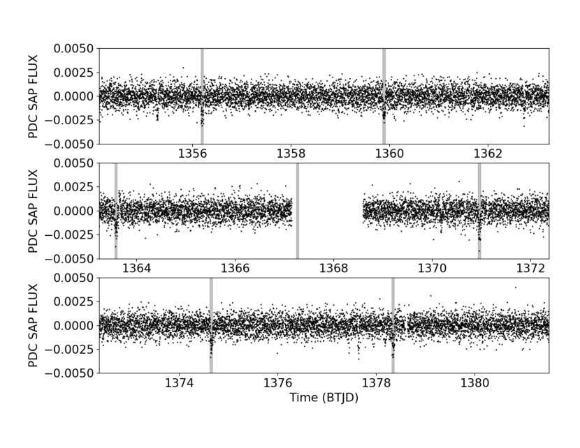
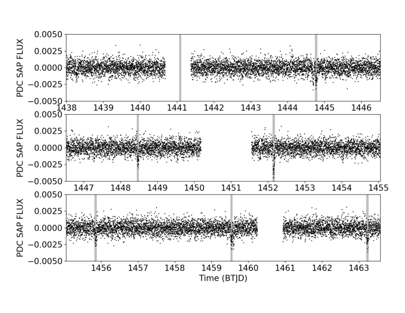
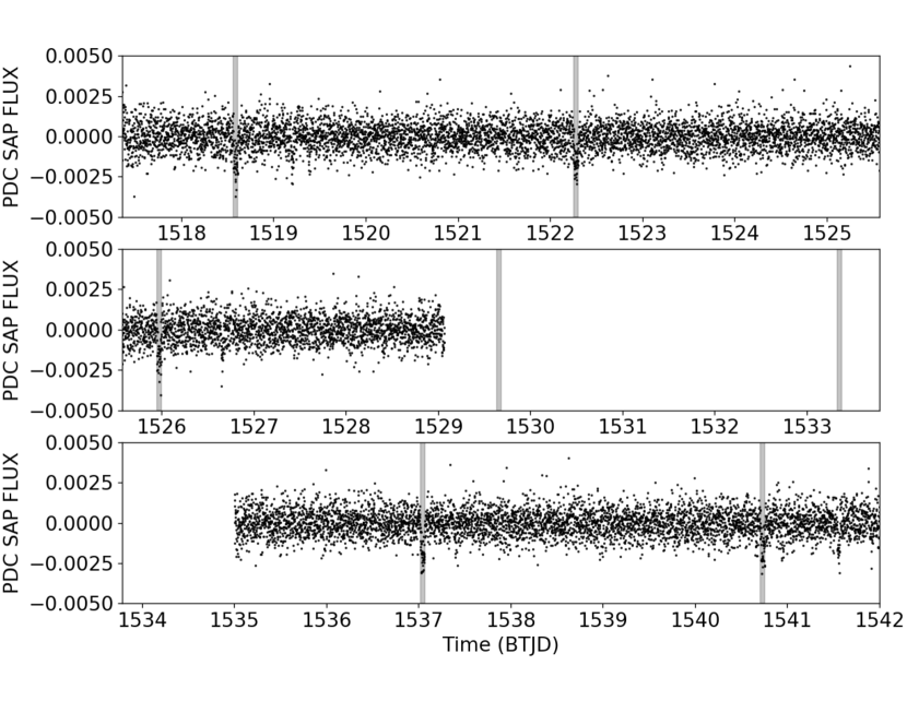
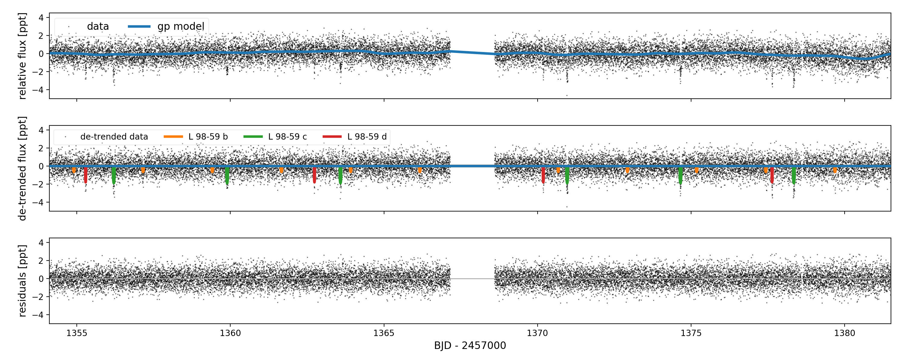
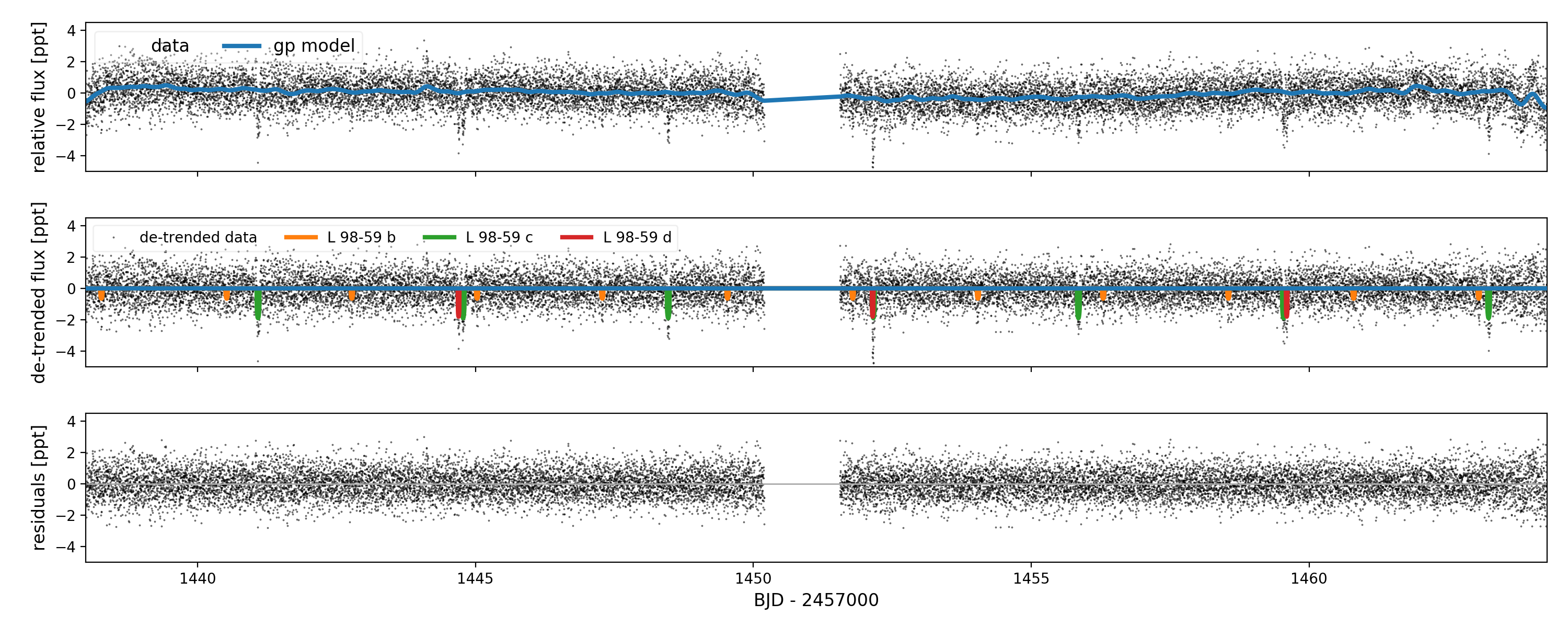
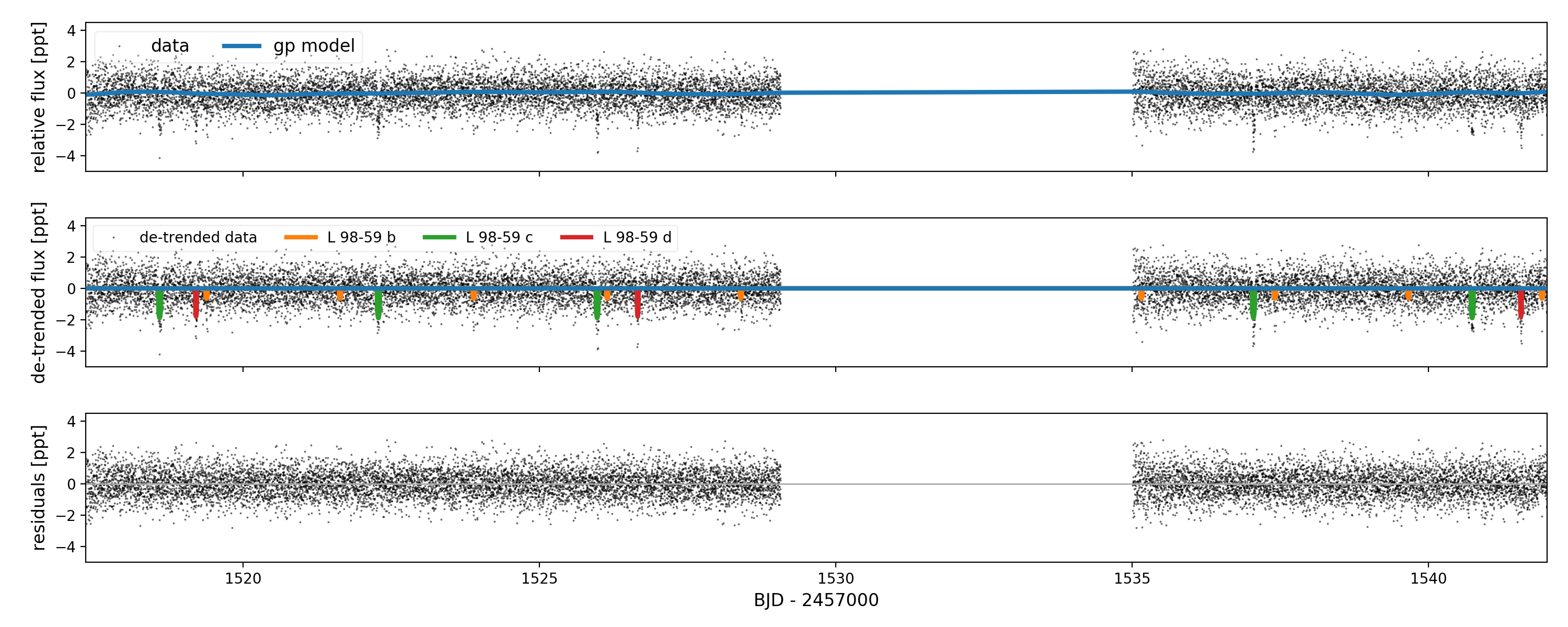
TESS observed L 98-59 (TIC 307210830, TOI-175; RA = 08:18:07.62, Dec = -68:18:46.80 (J2000)) in Sectors 2, 5, and 8 with Camera 4. The target was added to the TESS Candidate Target List—a list of targets prioritized for short-cadence observations (Stassun et al., 2018)—as part of the specially curated Cool Dwarf list (Muirhead et al., 2018). The TESS data were processed with the Science Processing Operations Center Pipeline (SPOC; Jenkins et al., 2016) and with the MIT Quick Look Pipeline. The three candidates identified by the SPOC pipeline passed a series of data validation tests (Twicken et al., 2018; Li et al., 2019) summarized below, and were made publicly available on the MIT TESS Data Alerts website²²2https://tess.mit.edu/alerts/ and the Mikulski Archive for Space Telescopes (MAST) TESS alerts page³³3https://archive.stsci.edu/prepds/tess-data-alerts/ as TOI-175.01, -175.02 and -175.03. These candidates had periods P = 3.690613 days, 7.451113 days, and 2.253014 days and transit epochs (BTJD) = 1356.203764, 1355.2864 and 1354.906208, respectively⁴⁴4BTJD = BJD - 2457000, and are referred to in the rest of the manuscript as L 98-59 c, L 98-59 d, and L 98-59 b respectively. The SPOC simple aperture photometery (SAP) and pre-search data conditioned (PDCSAP) lightcurves (Smith et al., 2012; Stumpe et al., 2014) of L 98-59 are shown in Figure 1.

Refer to caption — Figure 1: TESS PDCSAPFLUX lightcurves for L 98-59 as a function of time. Upper three panels represent sector 2 data, middle three panels sector 5, and lower panels—sector 8. For context, the transits of planet candidate L 98-59 c are indicated with vertical grey lines. As L 98-59 c and L 98-59 d are just wide of a 2:1 period resonance, their transits can sometimes occur close to each other (e.g. around days 1445 and 1459.5), and can even create a syzygy—like near day 1452.2.

We use the methods appropriate for M dwarfs previously used by (Berta-Thompson et al., 2015; Dittmann et al., 2017; Ment et al., 2018) to determine the stellar parameters of the host star, and adopt these parameters throughout our analysis. We estimate the mass of the star using the mass-luminosity relation in the $K-$ band from Benedict et al. (2016) to be 0.313 $\pm$ 0.014 M_⊙. We then use single star mass-radius relations (Boyajian et al., 2012) to find a stellar radius of 0.312 $\pm$ 0.014 R_⊙. We calculate the bolometric correction in $K$ from Mann et al. (2015, erratum) to be 2.7 $\pm$ 0.036 mag, resulting in a bolometric luminosity for L 98-59 of 0.011 $\pm$ 0.0004 L_⊙. We calculate the correction in $V$ from Pecaut & Mamajek (2013) to be -2.0 $\pm$ 0.03 mag⁵⁵5We assume the uncertainty on the bolometric correction in $V$ is that of the ( $V-K$ ) color., resulting in a bolometric luminosity of 0.0115 $\pm$ 0.0005 L_⊙. We adopt the mean of the two bolometric luminosities from which we calculate the luminosity of the host star to be 0.0113 $\pm$ 0.0006 L_⊙ (i.e. 4.31e24 W). From the Stephan-Boltzmann Law, we find an effective temperature ${\rm T_{eff}=3367\pm 150K}$ . As a comparison, we also used the relations in Mann et al. (2015) to determine an effective temperature of 3419 $\pm$ 77 K for L 98-59, in agreement with the $T_{eff}$ derived from the Stefan-Boltzmann Law.

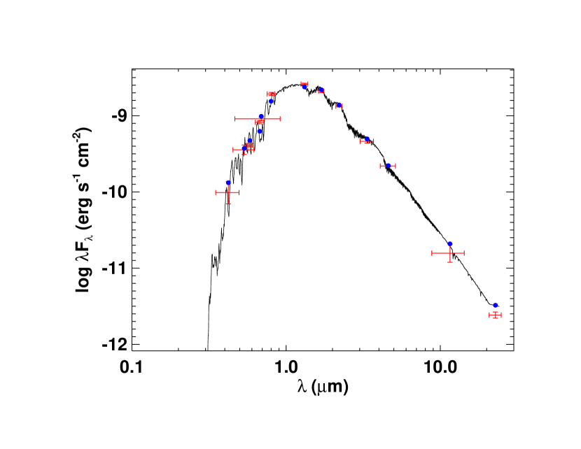
In addition, following the procedures described in Stassun & Torres (2016) and Stassun et al. (2017) to fit a NextGen stellar atmosphere model (Hauschildt et al., 1999) to broadband photometry data from Tycho-2, Winters et al. (2015), Gaia, 2MASS, and WISE, we performed a full fit of the stellar spectral energy distribution (SED) to estimate the stellar $T_{\rm eff}$ and [Fe/H] which, together with the Gaia DR2 parallax, provides an estimate of the stellar radius. The free parameters of the fit were $T_{\rm eff}$ and stellar metallicity [Fe/H], and we set the extinction $A_{V}\equiv 0$ due to the very close distance of the system. The resulting best fit is shown in Figure 2, with a reduced $\chi^{2}$ of 3.8 for 8 degrees of freedom. The best fit parameters are $T_{\rm eff}=3350\pm 100$ K and [Fe/H] $=-0.5\pm 0.5$ . Integrating the SED gives the bolometric flux at Earth as $F_{\rm bol}=2.99\pm 0.18\times 10^{-9}$ erg s^-1 cm^-2. Finally, adopting the Gaia DR2 parallax and the correction of 80 $\mu$ as from Stassun & Torres (2018), we calculate a stellar radius of $0.305\pm 0.018$ R_⊙ using the Stefan-Boltzmann law. These are consistent with the adopted parameters discussed above.

We also estimated a prior on the stellar density ( $\rho_{*}$ ) by estimating the stellar mass. Here we used the empirical relations of Mann et al. (2015), which provides $M_{star}\approx 0.32M_{\odot}$ from the absolute $K_{S}$ magnitude ( $M_{K_{S}}$ ) determined from the observed 2MASS $K_{S}$ magnitude and the Gaia DR2 parallax (corrected for the offset from Stassun & Torres, 2018). The quoted uncertainty in the Mann et al. empirical relation is $\sim$ 3%; here we conservatively adopt an uncertainty of 10%. Together with the radius determined above from the SED and parallax, we obtain $\rho_{*}=15.9\pm 3.3$ g cm^-3 (this value is used as a prior in the transit model). We also determined the stellar temperature and radius using empirical relations calibrated using low-mass stars with interferometrically measured radii and precise distances (see Feinstein et al., 2019, and references therein). These alternative stellar parameter estimates were consistent with those determined from the empirical M-dwarf relations and from the SED fitting. An additional set of stellar parameters for L 98-59 were previously derived from a medium-resolution optical spectrum in the CONCH-SHELL survey (Gaidos et al., 2014). This work also provides parameters consistent with our estimates. We compile the stellar parameters used in subsequent analyses and other identifying information for L 98-59 in Table 1. While it is difficult to pin down the ages of old M dwarfs due to their long main-sequence lifetime, the lack of a rapid rotation signal in the TESS SAP light curve and the low activity of L 98-59 (see § 2.4) indicate that it is likely an old M dwarf with an age $>$ 1 Gyr. The stellar parameters of L 98-59 are consistent with a spectral type of M3 $\pm$ 1.

Table 1: Stellar Parameters

Parameter	Value	Notes
Identifying Information
Name	L 98-59
TIC ID	307210830
TOI ID	175
$\alpha$ R.A. (hh:mm:ss)	08:18:07.62	Gaia DR2
$\delta$ Dec. (dd:mm:ss)	-68:18:46.80	Gaia DR2
$\mu_{\alpha}$ (mas yr^-1)	$94.767\pm 0.054$	Gaia DR2
$\mu_{\delta}$ (mas yr^-1)	$-340.470\pm 0.052$	Gaia DR2
Distance (pc)	$10.623\pm 0.003$	Gaia DR2
Photometric Properties
$B$ (mag) ……….	$13.289\pm 0.027$	APASS DR9
$V$ (mag) ……….	$11.685\pm 0.017$	APASS DR9
$G$ (mag) ……….	$10.598\pm 0.001$	Gaia DR2
$g^{\prime}$ (mag) ……….	$12.453\pm 0.019$	APASS DR9
$r^{\prime}$ (mag) ……….	$11.065\pm 0.044$	APASS DR9
$T$ (mag) ……….	9.393	TIC
$J$ (mag) ……….	$7.933\pm 0.027$	2MASS
$H$ (mag) ……….	$7.359\pm 0.049$	2MASS
$K_{s}$ (mag) ………	$7.101\pm 0.018$	2MASS
$W1$ (mag) ………	$6.935\pm 0.062$	ALLWISE
$W2$ (mag) ………	$6.767\pm 0.021$	ALLWISE
$W3$ (mag) ………	$6.703\pm 0.016$	ALLWISE
$W4$ (mag) ………	$6.578\pm 0.047$	ALLWISE
Stellar Properties
Spectral Type ……….	M3V $\pm$ 1	This Work
$T_{\mathrm{eff}}$ (K) ……….	$3367\pm 150$	This Work
$[$ Fe/H $]$ ……….	$-0.5\pm 0.5$	This Work
$M_{star}$ ( $M_{\odot}$ ) ……….	$0.313\pm 0.014$	This Work
$R_{star}$ ( $R_{\odot}$ ) ……….	$0.312\pm 0.014$	This Work
$L_{star}(L_{\odot})$ ……….	$0.0113\pm 0.0006$	This Work

^†^†footnotetext: Gaia DR2 - (Gaia Collaboration et al., 2018), UCAC5 - (Zacharias et al., 2017), APASS DR9 - (Henden et al., 2016), 2MASS - (Skrutskie et al., 2006), ALLWISE - (Cutri et al., 2013)

2.2 Lightcurve Analyses

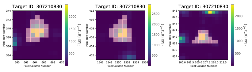
We opted to create our own apertures from Sectors 2, 5 and 8 target pixel file data to analyze the photometric time-series from TESS, instead of using the pipeline apertures used to first identify the transiting planet candidates. Our primary motivation for performing our own photometry is that we can avoid any attenuation to the transit signals by explicitly masking them during the systematic correction step. We first used the lightkurve package (Lightkurve Collaboration et al., 2018)⁶⁶6https://github.com/KeplerGO/lightkurve to extract lightcurves from each of the three sectors using the threshold method, which selects pixels that (a) are a fixed number of standard deviations above the background, and (b) create a contiguous region with the central pixel in the mask. We used a threshold value of 3 $\sigma$ ; the corresponding mask shape is shown in Figure 3. Thus produced, the resulting lightcurve still contains low-level instrumental systematic signals. To identify and subtract instrumental signals, we used a second order pixel-level de-correlation (PLD), which is a technique based on Spitzer and K2 analysis methods (Deming et al., 2015; Luger et al., 2016). During the PLD step, we masked out transits to avoid attenuating the signals. Finally, we normalized the lightcurve by dividing by the median and subtracting one to center the flux about zero. We did the PLD detrending separately for each sector.

We used the exoplanet toolkit for probabilistic modeling of the exoplanet transits (Foreman-Mackey, 2018). The model we built consisted of four elements: three planet transit components with Keplerian orbits and limb-darkened transits, and a Gaussian Process (GP) component that models residual stellar variability. The planet models were computed with exoplanet using STARRY (Luger et al., 2018), while the GP was computed using celerite (Foreman-Mackey et al., 2017; Foreman-Mackey, 2018). The GP component is described as a stochastically-driven, damped harmonic oscillator with parameters of $\log(S_{0})$ and $\log(\omega_{0})$ , where the power spectrum of the GP is

S(\omega)=\sqrt{\frac{2}{\pi}}\frac{S_{0}\,\omega_{0}^{4}}{(\omega^{2}-\omega_{0}^{2})^{2}+\omega^{2}\,\omega_{0}^{2}/Q^{2}},

(1)

and a white noise term, with a model parameter of the log variance. We fixed Q to $1/\sqrt{2}$ and put wide Gaussian priors on $\log(S_{0})$ and $\log(\omega_{0})$ with means of the log variance, and one log of one tenth of a cycle, respectively, and a standard deviation on the priors of 10. For each Sector we used separate GP parameters. This form of GP was chosen because of the flexible nature and smoothly varies (it is once mean square differentiable) enables us to use it to model a wide range of low frequency astrophysical and instrumental signals. The white noise term carried the same prior as $\log(S_{0})$ . Each sector of data had a separate parameter for the mean flux level.

The planet model was parameterized in terms of consistent limb darkening, log stellar density, and stellar radius for the three planets. Each individual planet was parameterized in terms of log orbital period, time of first transit, log planet-to-star radius ratio, impact parameter, orbital eccentricity and periastron angle at time of transit. The stellar radius had a Gaussian prior with mean 0.312 and 0.014 standard deviation, with solar units, and is additionally required to be positive. The log mean stellar density, in cgs units, had a Gaussian prior with a mean of $\log{15}$ and standard deviation of 0.2 dex (as per Section 2.1). The limb darkening followed the Kipping (2013a) parameterization.

The log orbital periods, time of first transits, and log planet-to-star radius ratio of the three planets had Gaussian priors with means at the values found in the TESS alert data, and standard deviations of 0.1, 0.1, and 1, respectively. The impact parameter had a uniform prior between zero and one plus the planet-to-star radius ratio. Eccentricity had a beta prior with $\alpha=0.867$ and $\beta=3.03$ (as suggested by Kipping, 2013b), and was bounded between zero and one. The periastron angle at transit was sampled in vector space to avoid the sampler seeing a discontinuity at values of $\pi$ .

We sampled the posterior distribution of the model parameters using the No U-turn Sampler (NUTS, Hoffman & Gelman, 2014) which is a form of Hamiltonian Monte Carlo, as implemented in PyMC3 (Salvatier et al., 2016). We ran 4 simultaneous chains, with 5000 tuning steps, and 3000 draws in the final sample. The effective number of independent samples of every parameter was above 1000, and most parameters were above 5000. The Gelman–Rubin diagnostic statistic was within 0.005 of 1.000 for each parameter in the model. The impact parameter for the outer planet is relatively high, which caused this parameter along with the orbital eccentricity to be most time consuming to sample independently.

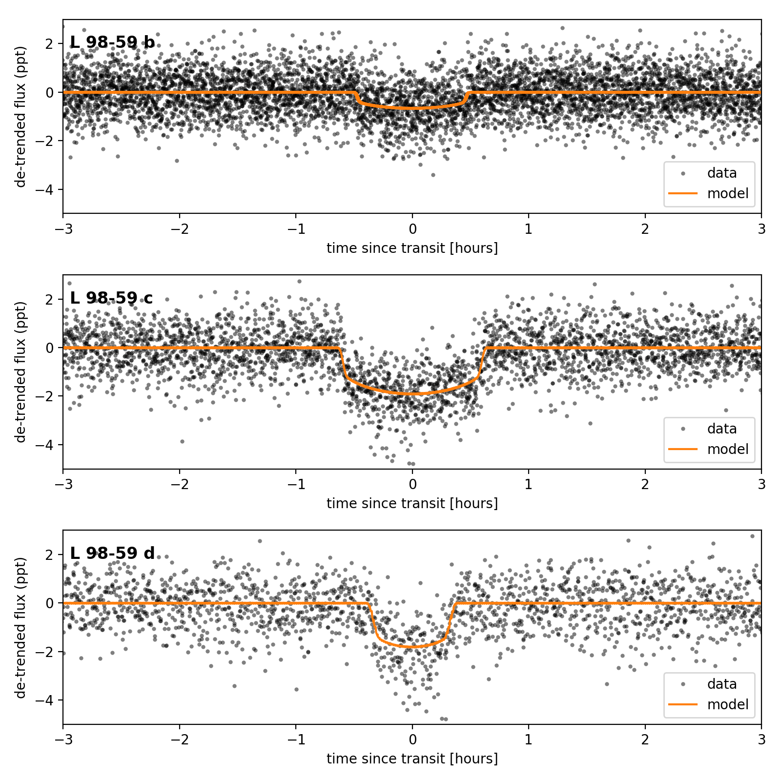
Figure 4 shows the GP model of the low-level variability in the upper panels, and the best fitting transit model in the central panels. The phase-folded transits of the three candidates, along best-fitting transit models, are shown in Figure 5, and the model parameters are provided in Table 2. The transit modeling reveals that the candidate planets have small radii ranging from 0.8 to 1.6 $R_{\oplus}$ . A chain of small terrestrial-sized planets is common among M-dwarfs (Muirhead et al., 2015), and L 98-59 is reminiscent of other systems such as the TRAPPIST-1, Kepler-186 and Kepler-296 (Gillon et al., 2017; Barclay et al., 2015; Quintana et al., 2014). The stellar density obtained from the transit model is fully consistent with that determined from the stellar parameters in Section 2.1 ( ${\rm 15.8^{+2.6}_{-2.7}~{}g~{}cm^{-3}}$ for the former vs ${\rm 15.9\pm 3.3~{}g~{}cm^{-3}}$ for the latter.

Table 2: Planet Parameters

Parameter	-1 $\sigma$	Median	+1 $\sigma$
Model Parameters
Star
$\ln{\rho}$ [g cm^-3]	2.57	2.76	2.91
Limb darkening $q_{1}$	0.41	0.65	0.83
Limb darkening $q_{2}$	-0.34	-0.11	0.28
L 98-59 b
${T_{0}}$ (BJD - 2457000)	1366.1694	1366.1701	1366.1707
$\ln{Period}$ [days]	0.812318	0.812326	0.812334
Impact parameter	0.13	0.36	0.55
$\ln{R_{p}/R_{*}}$	-3.79	-3.75	-3.72
eccentricity	0.03	0.10	0.27
$\omega$ [radians]	-2.2	0.3	2.4
L 98-59 c
${T_{0}}$ (BJD - 2457000)	1367.2752	1367.2755	1367.2759
$\ln{Period}$ [days]	1.305791	1.305795	1.305798
Impact parameter	0.09	0.29	0.49
$\ln{R_{p}/R_{*}}$	-3.25	-3.23	-3.20
eccentricity	0.02	0.09	0.25
$\omega$ [radians]	-2.5	-0.4	2.2
L 98-59 d
${T_{0}}$ (BJD - 2457000)	1362.7367	1362.7375	1362.7382
$\ln{Period}$ [days]	2.008323	2.008329	2.008334
Impact parameter	0.75	0.89	0.93
$\ln{R_{p}/R_{*}}$	-3.16	-3.07	-3.01
eccentricity	0.04	0.20	0.52
$\omega$ [radians]	-1.9	0.7	2.3
Derived Parameters
L 98-59 b
Period [days]	2.25312	2.25314	2.25316
${R_{p}/R_{*}}$	0.0226	0.0234	0.0243
Radius ${[R_{\oplus}]}$	0.75	0.80	0.85
Insolation	19.5	23.9	29.2
${a/R_{*}}$	15.2	16.2	17.0
$a$ [AU]	0.0216	0.0233	0.0250
Inclination (deg)	88.0	88.7	89.5
Duration (hours)	0.89	1.02	1.19
L 98-59 c
Period [days]	3.690607	3.690621	3.690634
${R_{p}/R_{*}}$	0.0388	0.0396	0.0407
Radius ${[R_{\oplus}]}$	1.28	1.35	1.43
Insolation	10.1	12.4	15.2
${a/R_{*}}$	21.1	22.5	, 23.6
$a$ [AU]	0.0300	0.0324	0.0347
Inclination (deg)	88.8	89.3	89.7
Duration (hours)	1.07	1.24	1.36
L 98-59 d
Period [days]	7.45081	7.45086	7.45090
${R_{p}/R_{*}}$	0.0426	0.0462	0.0492
Radius ${[R_{\oplus}]}$	1.43	1.57	1.71
Insolation	3.96	4.85	5.93
${a/R_{*}}$	36.2	37.4	38.5
$a$ [AU]	0.048	0.052	0.056
Inclination (deg)	88.0	88.5	88.7
Duration (hours)	0.74	0.91	1.68

We repeated this analysis using the systematics-corrected light curves from the TESS pipeline (PDCSAP Jenkins et al., 2016; Stumpe et al., 2014) rather than using the respective target pixel files. We found consistent results, aside from different GP parameters owing to the different systematics corrections applied. The transits depths were lower in the PDCSAP data at the ${\rm<1\sigma}$ level, which we attribute to masking out transits in the systematics-correction technique we applied. We did not include any flux contamination from nearby stars in our models because there are no bright nearby stars to contaminate our pixel mask – the TIC estimates that the contamination fraction for L 98-59 is 0.002. Even if the TIC contamination is dramatically underestimated, it is highly likely that the stellar radius uncertainty will be the dominant term in the planet radius uncertainty, therefore we feel comfortable neglecting it.

There are significant impact parameter differences between the inner two planets and the outer planet. The outer planet transits close to the limb of the star, although it is not grazing. This manifests in the light curve as a shorter transit duration for the outer planet than the two inner planets and indicates a modest mutual inclination of at least one degree between the inner two and outer planets. All three planets are subject to significantly more flux than Earth receives from the Sun, and are therefore unlikely to be good astrobiology targets. However, with an insolation flux of $4.5\pm 0.8$ , the outer planet is a candidate Venus-zone planet (Kane et al., 2014).

2.3 Potential false positive scenarios

The TESS Data Validation Report performs a series of tests designed to rule out various false positive scenarios. The results from these tests are as follows:
i) L 98-59 c and L 98-59 d pass the difference image centroiding test, which employs PSF-based centroiding on the difference images (expected to be more precise and accurate than a brightness-weighted moment on the difference images). While L 98-59 b does not quite pass the difference image centroiding test, its transits are much shallower compared to the other two candidates. Thus it is likely that the centroiding errors are underestimated to some degree due to the variable pointing performance at timescales less than the 2 minutes observation cadence. We expect the analysis of this candidate to improve with new data;
ii) All three candidates pass the odd-even difference tests; iii) Secondary eclipses are ruled out at the 3.6-, 2.6- and 1.8- ${\sigma}$ levels;
iv) A bootstrap analysis of the out-of-transit data is used to quantify the probability of false alarms due to stellar variability and residual instrumental systematics. In the case of L 98-59, the light curve is well behaved and the analysis excludes the possibility of a false alarm at the 2.45E-25, 6.6E-62, and 2.2E-25 levels (as extrapolations of the upper tail of the bootstrap distribution to the observed maximum Multiple Event Statistics (MES) that triggered the detections of these candidates in the pipeline (Jenkins et al., 2017));
v) All three candidates pass a ghost diagnostic test, designed to flag instances of scattered light, other instrumental artifacts or background eclipsing binaries.

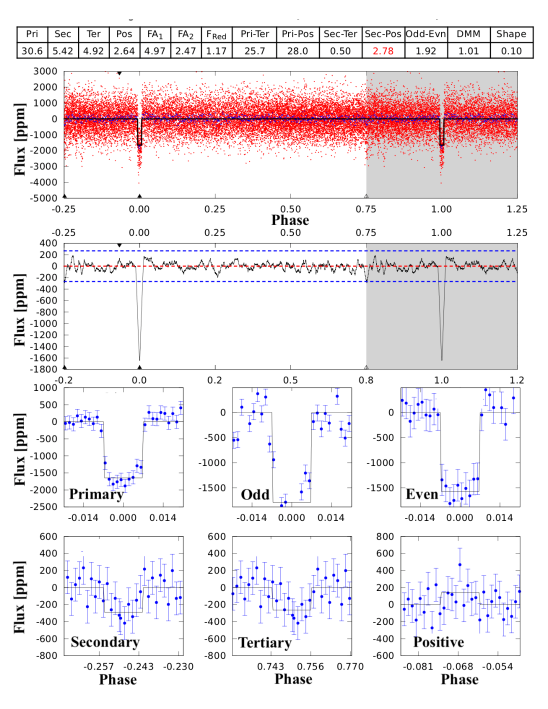
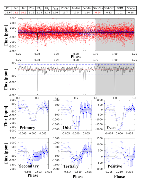
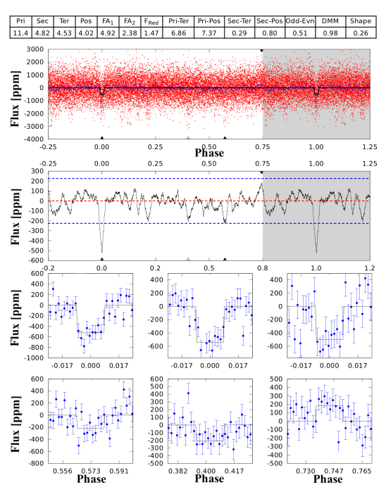
For completeness, we also applied the vetting pipeline DAVE (Kostov et al., 2019) to the TESS lightcurve of L 98-59. Briefly, DAVE evaluates whether detected transit-like events produced by the candidate are real or false positives by analyzing the data for (a) odd-even differences between consecutive transits; (b) secondary eclipses; (c) stellar variability mimicking a transit; and (d) photocenter shifts during transit;

To perform the (a), (b) and (c) analysis we used the Modelshift module of DAVE—an automated package designed to emphasize features in the lightcurve that resemble the shape, depth and duration of the planetary transit but located at different orbital phase. To identify secondary eclipses and odd-even transit differences, or flares and heartbeat stars (Welsh et al., 2011, see e.g.), Modelshift first convolves the lightcurve with the transit model of the planet candidate. The module then computes the significance of the primary transits, odd-even differences, secondary, tertiary and positive features assuming white noise in the lightcurve, and compares the ratio between each of these and the systematic red noise ${\rm F_{red}}$ to the false alarm thresholds ${\rm FA_{1}=\sqrt{2}erfcinv(T_{dur}/(P\times N))}$ (assuming 20,000 objects evaluated), and ${\rm FA_{2}=\sqrt{2}erfcinv(T_{dur}/P)}$ (for two events), where ${\rm T_{dur},P,N}$ are the duration, period and number of events (see Coughlin et al. 2014 for details). For example, a secondary feature is considered significant if ${\rm Sec/F_{red}>FA_{1}}$ . The Modelshift results are shown in Figures 6, 7, and 8 where the panels show the phase-folded lightcurve (first row), the phase-folded lightcurve convolved with the best-fit transit model (second row), as well as the the best-fit to all primary transits, all odd and all even transits, the most prominent secondary, tertiary and positive features in the lightcurve (lower two rows). The tables above the figures list the individual features evaluated by the module: the significance of the primary (“Pri”), secondary (“Sec”), tertiary (“Ter”) and positive (“Pos”) events assuming white noise, along with their corresponding differences (“Pri-Ter”, “Pri-Pos”, “Sec-Ter”, “Sec-Pos”), the significance of the odd-even metric (“Odd-Evn”), the ratio of the individual depths’ median and mean values (“DMM”), the shape metric (“Shape”), the False Alarm thresholds (“ ${\rm FA_{1}}$ ”, “ ${\rm FA_{2}}$ ”), and the ratio of the red noise to the white noise in the phased light curve at the transit timescale (“Fred”). Our analysis shows that there are no secondary eclipses or odd-even differences for any of the L 98-59 planet candidates. We note that the significant secondary and tertiary eclipses identified by DAVE for L 98-59 d (Figure 7) are due to the transits of L 98-59 c and thus not a source of concern.

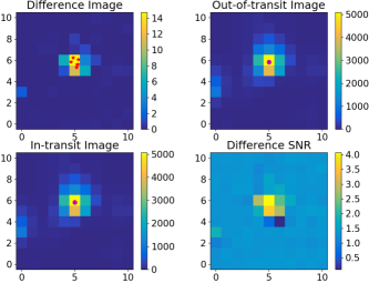
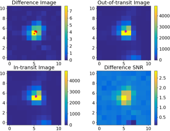
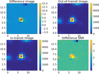
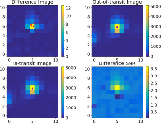
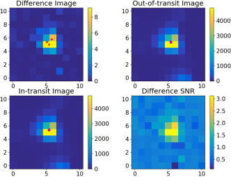
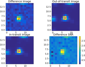
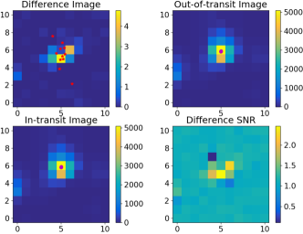
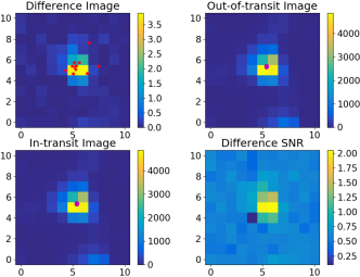
To perform the (d) analysis for each candidate we used the photocenter module of DAVE, following the prescription of Bryson et al. (2013). Specifically, for each candidate we: 1) create the mean in-transit and out-of-transit images for each transit (ignoring cadences with non-zero quality flags), where the latter are based on the same number of exposure cadences as the former, split evenly before and after the transit; 2) calculate the overall mean in-transit and out-of-transit images by averaging over all transits; 3) subtract the overall mean out-of-transit image from the overall in-transit image to produce the overall mean difference image; and 4) measure the center-of-light for each difference and out-of-transit image by calculating the corresponding $x$ - and $y$ -moments of the image. The measured photocenters for the three planet candidates are shown in Figures 9, 10, and 11, and listed in Table 3. We detect no significant photocenter shifts between the respective difference images and out-of-transit images for any of the planet candidates (see Table 3), which confirms that the target star is the source of the transits. We note that some of the individual difference images for L 98-59 b deviate from the expected Gaussian profile, and thus so does the mean difference image.

Table 3: Photocenter Analysis of the three planet candidates

Parameter	Row [pixels]	Column [pixels]
L 98-59 b
Out of Transit Image Centroid	$338.83\pm 0.02$	$664.01\pm 0.01$
Difference Image Centroid	$338.34\pm 1.39$	$664.04\pm 0.55$
Offset	$-0.49\pm 1.39$	$0.03\pm 0.55$
Offset/ $\sigma$	0.35	0.05
L 98-59 c
Out of Transit Image Centroid	$338.83\pm 0.02$	$664.01\pm 0.01$
Difference Image Centroid	$338.76\pm 0.31$	$664.11\pm 0.24$
Offset	$-0.07\pm 0.31$	$0.1\pm 0.24$
Offset/ $\sigma$	0.23	0.42
L 98-59 d
Out of Transit Image Centroid	$338.93\pm 0.02$	$664.02\pm 0.02$
Difference Image Centroid	$339.27\pm 0.21$	$664.06\pm 0.34$
Offset	$0.34\pm 0.21$	$0.04\pm 0.34$
Offset/ $\sigma$	1.62	0.12

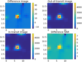
Overall, our DAVE results rule out false-positive features for all three planet candidates of L 98-59, are consistent with the analysis of the Data Validation Report, and indicate that the detected events are genuine transits associated with the star in question. We also note that while the automated vetting of Osborn et al. (2019) flagged L 98-59 with “a high likelihood of being astrophysical false positives” (their Table 3), their subsequent manual vetting lists the system as planet candidate.

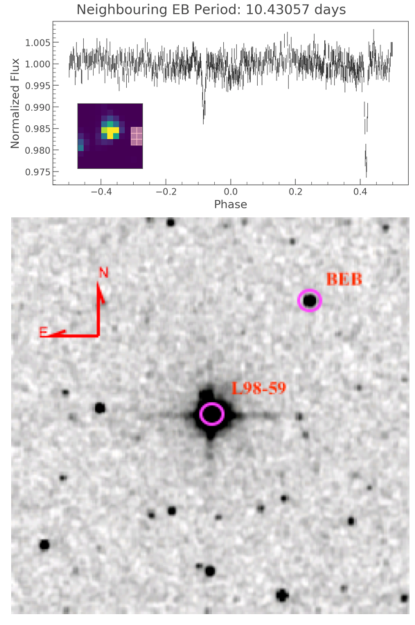
Additionally, to investigate whether one or more of the transits associated with L 98-59 may result from nearby sources (e.g. a background eclipsing binary), we used lightkurve to extract lightcurves for nearby field stars. Our analysis revealed that a nearby field star ${\sim 80\arcsec}$ NW of L 98-59 (2MASS 08175808-6817459, TIC 307210817, Tmag = 13.45, i.e. $\approx 4$ magnitudes fainter than L 98-59) is in fact an eclipsing binary (EB), manifesting both primary and secondary eclipses at a period of ${\approx 10.43}$ days, with ${T_{0}=4.4309}$ (BJD-2,455,000) (see Figure 12). This field star could be associated with one of two sources in the Gaia catalog: Source 1 with RA = 124.49217149500, Dec = -68.29612321000, ID = 5271055685541797120, and parallax=0.1888 mas; and Source 2 with RA = 124.49126472300, Dec = -68.29602748080, ID = 5271055689840223744, and parallax = 0.9977 mas. Given the corresponding approximate distances of 1 and 5 kpc, neither of these targets can be physically associated with L 98-59 as they lie deep in the background. Regardless of which of these sources hosts the detected EB, the faintness of the host compared to L 98-59, the measured EB orbital parameters, and the dilution-corrected eclipse depths are inconsistent with the properties of the candidate planets and effectively rule it out as the potential source of any of these signals.

2.4 Follow-up Observations

We pursued ground-based follow up of the three candidates to rule out potential sources of false positives and strengthen the evidence of their planetary nature. Our L 98-59 follow-up program was organized through the TESS Follow-up Observing Program (TFOP) Working Group (WG)⁷⁷7https://tess.mit.edu/followup/ which facilitates follow-up of TESS candidate systems. The primary goal of the TFOP WG is to provide follow-up observations that will advance the achievement of the TESS Level One Science Requirement to measure masses for 50 transiting planets smaller than 4 Earth radii. A secondary goal of the TFOP WG is to foster communication and coordination for any science coming out of TESS. Our L 98-59 follow-up was conducted by three TFOP Sub Groups (SGs): SG-1, seeing limited photometry; SG-2, reconaissance spectroscopy; and SG-3, high-resolution imaging.

2.4.1 Seeing-Limited Photometry from the TFOP WG

Analysis of multi-planet systems from Kepler has shown that these have a higher probability of being real planets (e.g., Lissauer et al., 2012), lending credibility to the planetary nature of the transit events associated with L 98-59. However, the pixel scale of TESS is larger than Kepler’s ( ${21\arcsec}$ for TESS vs. ${4\arcsec}$ for Kepler) and the point spread function of TESS could be as large as ${1\arcmin}$ , both of which increase the probability of contamination by a nearby eclipsing binary (EB). For example, a deep eclipse in a nearby faint EB might mimic a shallow transit observed on the target star due to dilution. Thus it is critical to explore the potential contamination of relatively distant neighbors in order to confirm transit events detected on a TESS target.

To identify potential false positives due to variable stars such as EBs up to ${2.5\arcmin}$ away from L 98-59, we made use of the TFOP SG1. Specifically, we observed the target with ground-based facilities at the predicted times of the planet transits to search for deep eclipses in nearby stars at higher spatial resolutions. We used the TESS Transit Finder, which is a customized version of the Tapir software package (Jensen, 2013), to schedule photometric time-series follow-up observations. The facilities we used to collect TFOP SG1 data are: Las Cumbres Observatory (LCO) telescope network (Brown et al., 2013); SPECULOOS South Observatory (SSO) (Delrez et al., 2018; Burdanov et al., 2018); MEarth-South telescope array (MEarth) (Irwin et al., 2015); and Siding Spring Observatory T17 (SSO T17). Detailed observation logs are provided in Table 4.

Table 4: Observation Log

Planet	Date	Telescope^${\dagger}$^${\dagger}$Telescopes: LCO-SSO-1: Las Cumbres Observatory - Siding Spring (1.0 m) LCO-CTIO-1: Las Cumbres Observatory - Cerro Tololo Interamerican Observatory (1.0 m) LCO-CTIO-0.4: Las Cumbres Observatory - Cerro Tololo Interamerican Observatory (0.4 m) LCO-SAAO-1: Las Cumbres Observatory - South African Astronomical Observatory (1.0 m) LCO-SAAO-0.4: Las Cumbres Observatory - South African Astronomical Observatory (0.4 m) SSO-Europa: SPECULOOS South Observatory - Europa (1.0 m) SSO-Io: SPECULOOS South Observatory - Io (1.0 m) SSO-T17: Siding Spring Observatory - T17 (0.4 m) MEarth: MEarth-South telescope array (0.4 m $\times$ 5 telescopes)	Filter	ExpT	Exp	Dur.	Transit	Aperture	FWHM
Planet	(UTC)		Filter	(sec)	(N)	(min)	coverage	(arcsec)	(arcsec)
b	2018-10-19	LCO-SSO^‡	r^′	120	41	147	Ingr.+71 $\%$	3.89	2.21
	2018-11-11	SSO-Europa	r^′	15	764	315	Full	5.25	4.53
	2018-11-11	LCO-CTIO-1	i^′	25	120	154	Full	5.83	3.49
	2018-11-18	LCO-SAAO-0.4^‡	i^′	70	125	175	Full	9.14	7.03
	2018-11-20	LCO-CTIO-1	r^′	30	146	178	Full	3.89	2.20
	2018-11-29	LCO-CTIO-1	r^′	30	186	223	Full	5.83	3.56
	2018-12-07	SSO-Io	r^′	15	998	415	Full	5.60	4.06
	2019-01-26	LCO-SAAO-1^‡	r^′	12	88	234	Full	3.89	3.08
c	2018-10-16	LCO-CTIO-1	i^′	20	63	70	Ingr.+30 $\%$	4.27	2.01
	2018-10-22^‡	SSO-T17	clear	30	122	86	Ingr.+77 $\%$	7.10	2.40
	2018-11-11	SSO-Europa	r^′	15	764	315	Full	5.25	4.53
	2018-11-22	MEarth	RG715	45	1682	380	Full	20.16	8.00
	2018-12-25	LCO-SSO-1	i^′	22	108	113	Full	5.05	1.89
	2019-01-20	LCO-CTIO-1	g^′	100	85	197	Full	6.22	2.75
	2019-01-20	LCO-CTIO-1	zs	30	170	197	Full	9.36	4.43
d	2018-11-07	LCO-CTIO-0.4	i^′	70	119	170	Full	6.85	4.48
	2018-11-22	LCO-CTIO-1^‡	i^′	25	108	113	Full	6.22	5.05
	2018-11-22	MEarth	RG715	45	1682	380	Full	20.16	8.00
	2019-01-13	LCO-CTIO-0.4	i^′	14	143	73	Full	5.14	2.32
	2019-01-20	LCO-CTIO-1	r^′	30	132	151	Full	6.22	2.89
	2019-01-28	LCO-CTIO-1	g^′	50	153	223	Full	7.78	2.35

^${\ddagger}$^${\ddagger}$footnotetext: Observations not shown in Figures 13, 14, and 15 due to intrinsically high scatter in the light curve and/or because they were a deep exposure search for eclipsing binaries in nearby stars.

We used the AstroImageJ software package (Collins et al., 2017) for the data reduction and the aperture photometry in most of these follow-up photometric observations. For the observations carried out at SSO, the standard calibration of the images and the extraction of the stellar fluxes were performed using the IRAF/DAOPHOT aperture photometry software as described in Gillon et al. (2013). The results are shown in Figures 13, 14 and 15.

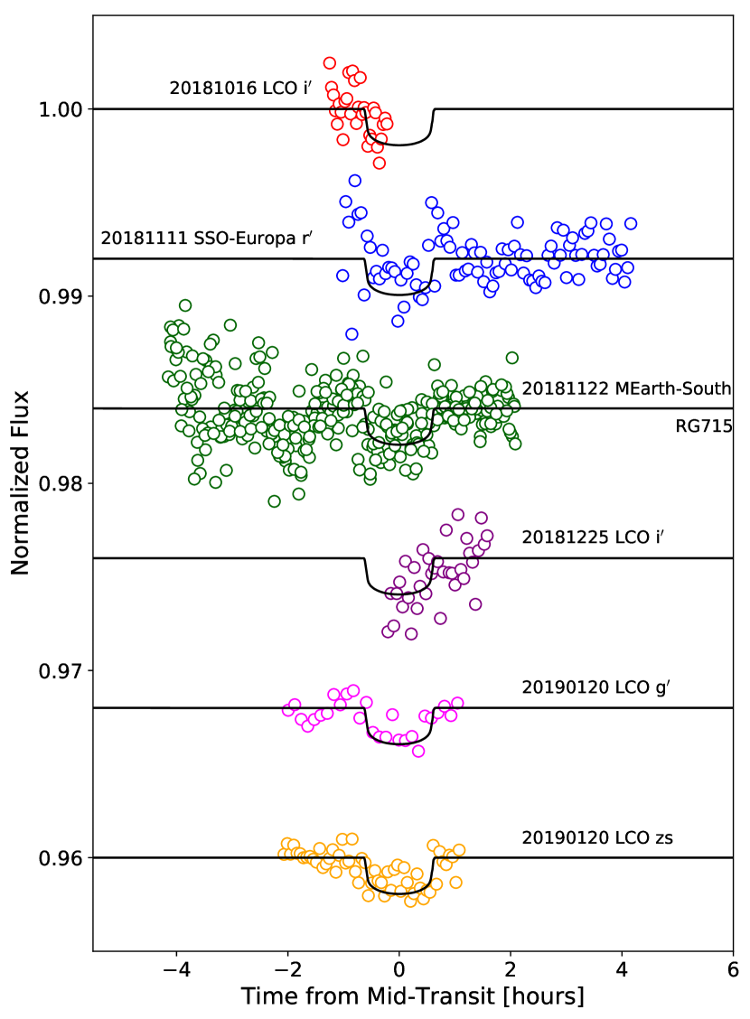
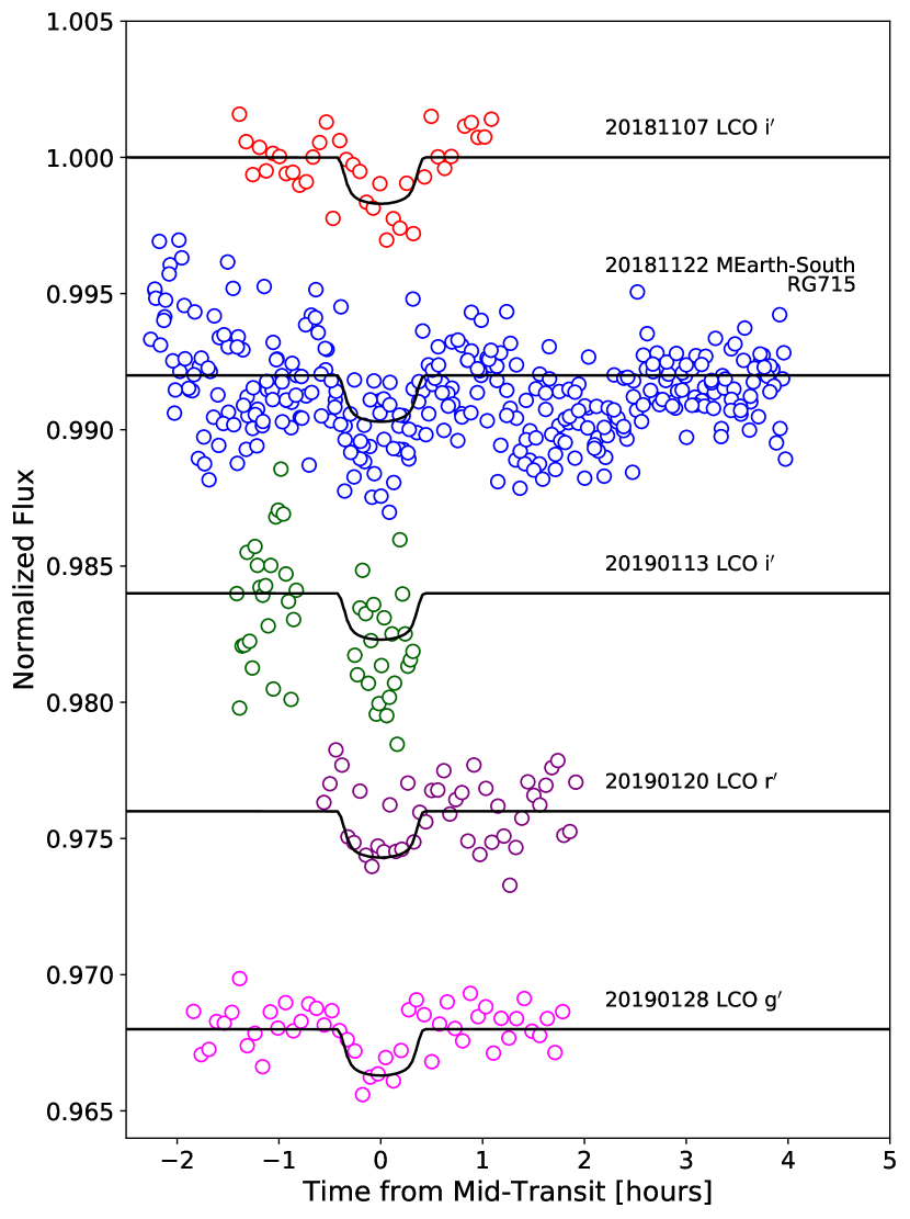
For all three planet candidates, we confirmed that the target star is the source of the transits, and ruled out nearby EBs which could mimic the transits. In addition, observations of L 98-59 c and d in different filters showed no chromatic dependence, which strengthens the hypothesis that the candidates are real planets. Our follow-up did detect a nearby EB at a separation of 54″ (TIC 307210845, Tmag = 16.042, i.e. $\sim 7$ magnitudes fainter than TIC 307210830, producing no detectable eclipses in the lightcurve of the latter), and we used deep exposures to confirm that it is not the origin of the L 98-59 b transits, providing high level of confidence about the planetary nature of this candidate.

The measured transit depths revealed by follow-up transit photometry are consistent with the transit depths measured from TESS. The differences in the follow-up and TESS transit depth measurements (in terms of $Rp/R*$ ) are listed in Table 5 as a function of wavelength, where we have included only the transits with scatter low enough to reasonably detect the events.

Table 5: Follow-up

{R_{p}/R_{*}}

minus TESS

{R_{p}/R_{*}}

as a function of wavelength

TOI	Date Obs	Filter (Observatory)	${R_{p}/R_{}}$ minus TESS ${R_{p}/R_{}}$
L 98-59 b	UT 2018-11-20	Sloan r’ (LCO)	$-0.0008^{+0.0054}_{-0.0085}$
L 98-59 b	UT 2018-11-29	Sloan r’ (LCO)	$0.0018^{+0.0039}_{-0.0045}$
L 98-59 c	UT 2019-01-20	Sloan g’ (LCO)	$-0.0033\pm 0.003$
L 98-59 c	UT 2018-11-22	RG715 (MEarth)	$-0.0007\pm 0.002$
L 98-59 c	UT 2019-01-20	Sloan z’ (LCO)	$-0.0056\pm 0.0028$
L 98-59 d	UT 2019-01-28	Sloan g’ (LCO)	$0.0072^{+0.0078}_{-0.0064}$
L 98-59 d	UT 2019-01-20	Sloan r’ (LCO)	$-0.003^{+0.01}_{-0.012}$
L 98-59 d	UT 2018-11-07	Sloan i’ (LCO)	$0.0072^{+0.0088}_{-0.0072}$
L 98-59 d	UT 2018-11-22	RG715 (MEarth)	$0.0104^{+0.0044}_{-0.0043}$

2.4.2 Reconnaissance Spectroscopy

To investigate the magnetic activity and rotation of L 98-59 and rule out spectroscopic binary companions, we obtained two epochs of optical spectra of L 98-59 on UT 2018 February 12⁸⁸8The first epoch of spectroscopic data were obtained as part of the M dwarf spectroscopic program described in Winters et al. (2019), before $TESS$ began observations. and on UT 2018 November 20 using the slicer mode with the CTIO HIgh ResolutiON (CHIRON) spectrograph (Tokovinin et al., 2013) (R $\simeq$ 80,000) on the Cerro Tololo Inter-American Observatory (CTIO)/ Small and Moderate Aperture Research Telescope System (SMARTS) 1.5m telescope. CHIRON has a spectral range of 410-870 nm. We obtained one 7.5-minute exposure for the first epoch and 3 $\times$ 2.5-minute exposures for the second observation, yielding a signal-to-noise ratio of roughly 13 in order 44 for both epochs. As described in Winters et al. (2018), we used an observed template of Barnard’s Star to derive a radial velocity of -5.8 $\pm$ 0.1 km s^-1 using the TiO molecular bands at 7065–7165 Å⁹⁹9We note that the total uncertainty on the systemic velocity should include the 0.5 km s^-1 uncertainty on the Barnard’s Star template velocity.. Our analyses of the spectra reveal no evidence of double lines. We see negligible rotational broadening ( $v$ sin $i$ = $0.0\pm 1.9$ km/s), and do not see H $\alpha$ in emission, providing evidence that the star is inactive and not host to unresolved, close-in, stellar companions. We are also able to rule out the presence of a brown dwarf companion to the host star. The radial velocity difference between the two observations, separated in time by roughly nine months, is 53 $\pm$ 52 m s^-1. For comparison, a 13 Jupiter-mass companion in a circular, nine-month period would induce a velocity semi-amplitude of 863 m s^-1 on this star. This semi-amplitude is eight times larger than our velocity uncertainty and would have been readily detectable. Thus, it is highly unlikely that there is a low-mass stellar or brown dwarf companion around L 98-59 at periods shorter than nine months.

We note, as well, that the trigonometric distance of 10.623 $\pm$ 0.003 pc from the Gaia second data release is in agreement with the photometric distance estimate of 12.6 $\pm$ 1.9 pc reported in Winters et al. (2019). Undetected equal-luminosity companions would contribute light to the system, making the system overluminous and resulting in an underestimated photometric distance estimate. Because the two distances are in agreement, this lends further support to the host star being a single star.

We also placed L 98-59 on an observational Hertzsprung-Russel color-magnitude Diagram (blue star; see Figure 16). Because it is not elevated above the main sequence or among the blended photometry binary sequence (red points), even more strength is given to the argument of this star being single.

In addition, we obtained a near-IR spectrum of L 98-59 on 2018 December 22 with the Folded-port InfraRed Echellete (FIRE) spectrograph (Simcoe et al., 2008) on the 6.5 Baade Magellan telescope at Las Campanas observatory. FIRE covers the 0.8-2.5 micron band with a spectral resolution of $R=6000$ . The target was observed under favorable conditions, with an average seeing of $\sim 0\farcs 6$ . L 98-59 was observed twice in the ABBA nod patterns at 40s integration time for each frame using the $0\farcs 6$ slit. Reductions and telluric corrections, using the nearby A0V standard HIP 41451, were completed with the FIREhose IDL package. We derived stellar parameters following the empirical methods derived by Newton et al. (2015). For L 98-59, we infer: $T_{eff}=3620\pm 74$ K, $R_{star}=0.37\pm 0.027R_{\odot}$ , and $L=0.021\pm 0.004L_{\odot}$ ., consistent with the SED analysis.

2.4.3 High Resolution Imaging

Photometric contamination from nearby sources can result in various false positive scenarios (e.g. background eclipsing binaries), and can bias the measured planetary radius from photometric analysis (see e.g. Ciardi et al., 2015; Furlan & Howell, 2017; Ziegler et al., 2018). In this work we use several high resolution images to tightly constrain the possible background sources and companion stars present near L 98-59. Previous speckle observations of the target were collected with Gemini/DSSI on 2018 March 31 as part of the M dwarf speckle program described in Winters et al. (2019). Once the candidate planets in this system had been identified by TESS, we collected additional speckle images with Gemini/DSSI (Horch et al., 2011) on 2018 November 01, and AO images with VLT/NaCo on 2019 January 28. Both epochs of Gemini/DSSI data are collected simultaneously through R and I band filters (692nm and 880nm respectively), while the VLT/NaCo data are collected in the Br $\gamma$ filter. At 0.5” from the host, these data rule out companions 5.0, 6.6 and 5.8 magnitudes fainter than the host star in the R, I and Br $\gamma$ bands respectively. The 5- $\sigma$ contrast curves for each of these observations are presented in Figure 17.

Due to the high proper motion of the target (354 mas/yr), the target undergoes significant motion even over the relatively modest time baseline of these observations. The on-sky position of the target is displaced by 338 mas between the observations on 2018 March 31 and 2019 January 28. This motion is significantly more than the PSF width in the high resolution images, and we are therefore able to rule out the presence of stationary background objects within $\sim$ 6 magnitudes of the host at any separation: any background objects obscured by the target in the first observation would be clearly visible in the final observation and vice versa. The motion of the target is demonstrated in Figure 17. These data also allow tight constraints to be placed on the presence of co-moving companions beyond $\sim$ 150 mas (=1.6 AU at the distance of this target). An object with $\Delta$ Br $\gamma\sim$ 6 mag and at the distance of L 98-59 would have a mass of $\sim 75$ M_J at an age of 10 Gyr (Baraffe et al., 2003)¹⁰¹⁰10Given the difficulty in estimating M-dwarf ages, we use an age of 10 Gyr so as to calculate a conservative mass limit., and we can therefore rule out any stellar companions to this host with a projected separation greater than 1.6 AU, while stellar companions closer than this could be easily detected in radial velocity data with a sufficient baseline.

Overall, the follow-up efforts demonstrate that there are tentative transit detections of the various candidates from the ground but it is difficult to confirm them since they are all shallow events. More importantly, none of these detections were identified as eclipsing binary scenarios (either on the host star or on nearby stars), supporting the planetary nature of the three transit candidates.

3 Discussion

Our lightcurve and false positive analyses, follow-up observations, and the multiplicity of the system provide strong evidence that the detected transit signals are planetary in nature. We consider the planets L 98-59b, c, and d to be a validated system of terrestrial planets orbiting a very nearby, bright M dwarf. Here we explore additional properties of the system to place constraints on the planet masses, orbital dynamics and evolution, and discuss their potential for future characterization.

3.1 Planet Mass Constraints

In the absence of radial velocity measurements, we placed constraints on the masses of the planets using the forecaster package for probabilistic mass forecasting (Chen & Kipping, 2017). From the mean and standard deviation of each planet’s radius, we generated a grid of 5000 masses within the entire mass range of the conditioned model, which spans dwarf planets to high-mass Jovians, and sampled 50000 times from a truncated normal distribution. For each sampled radius, forecaster computes a vector of probabilities given each element in the mass grid and a randomly chosen set of hyper-parameters from the hyper-posteriors of the model (which include transition points and intrinsic dispersion in the mass-radius relation). From this vector, the package returns the median mass and $\pm 1\sigma$ values. From the calculated radius values of 0.8 [0.05] ${R_{\oplus}}$ (L 98-59 b), 1.35 [0.07] ${R_{\oplus}}$ (L 98-59 c), and 1.57 [0.14] ${R_{\oplus}}$ (L 98-59 d), we determined mass values of 0.5 [+0.3, -0.2] ${M_{\oplus}}$ , 2.4 [+1.8, -0.8] ${M_{\oplus}}$ , and 3.4 [+2.7, -1.4] ${M_{\oplus}}$ , respectively. The large errors on these values suggest that better constrained radii from continued follow-up observations, combined with precise radial velocity measurements, are necessary to constrain the true masses. We note that given the brightness of the host star, the L 98-59 planets should be great targets for mass measurements to establish the M-R relation for M-dwarf planets. Using the forecaster masses, the expected radial velocity semi-amplitude, K, for the three planets are 0.54, 2.22, and 2.48 m/s for L 98-58 b, L 98-58 c, and L 98-58 d respectively—the outer two comparable to the amplitude of the measured radial velocity signal produced by e.g. GJ 581 b (Mayor et al., 2009) and Proxima Centauri b (Anglada-Escudé et al., 2016).

3.2 Dynamical stability and transit-timing variations

3.2.1 Long-Term Stability

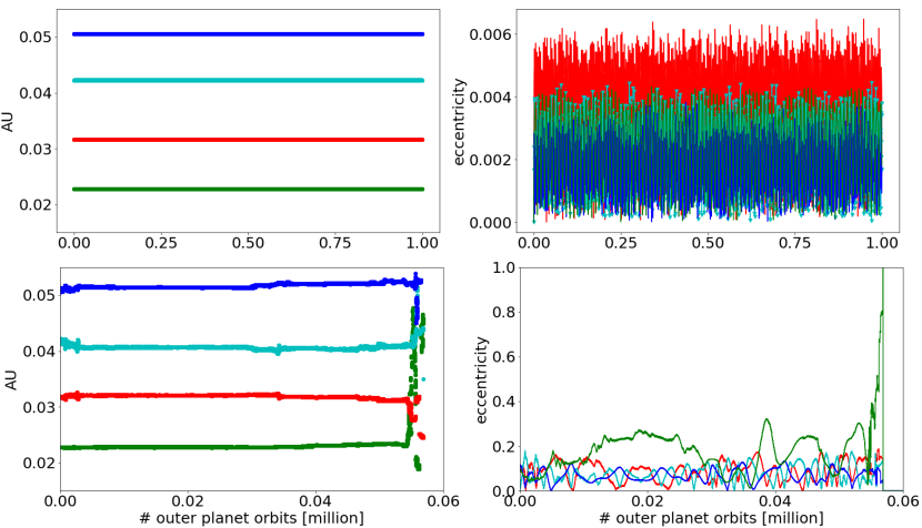
To examine the long-term dynamical stability and orbital evolution of the L 98-59 planets, we integrated the system using Rebound (Rein & Spiegel, 2015) for 1 million orbits of the outer planet ( ${\rm P=7.45}$ days). We used two sets of initial conditions – planets on circular orbits, and on eccentric orbits with $e=0.1$ – and start all integrations with randomly-selected initial arguments of periastron. Given the large uncertainties on the forecaster masses, we also tested the dynamical stability for two sets of planetary masses: best-fit masses (i.e. 0.5 ${M_{\oplus}}$ , 2.4 ${M_{\oplus}}$ and 3.4 ${M_{\oplus}}$ for L 98-58 b, L 98-58 c and L 98-58 d respectively), and best-fit+ ${1\sigma}$ masses (i.e. 0.58 ${M_{\oplus}}$ , 4.2 ${M_{\oplus}}$ and 6.1 ${M_{\oplus}}$ for L 98-58 b, L 98-58 c and L 98-58 d respectively). Overall, we performed 1000 numerical simulations for each set of planetary masses, using the IAS15 non-symplectic integrator (Rein & Spiegel, 2015) with a timestep of 0.01 the orbit of the inner planet (i.e. about 30 min).

Our simulations show that for initially circular orbits, the semi-major axes and eccentricities do not exhibit extreme variations, the system does not exhibit chaotic behavior for the duration of the numerical integrations for either set of planet masses, and the orbits remain practically circular (Figure 18). In contrast, for initially eccentric orbits with $e=0.1$ , the system becomes unstable in half of our simulations (with randomly-selected initial arguments of periastron), both for the best-fit and the best-fit+ ${1\sigma}$ planet masses (Figure 19). Thus we consider orbits with non-negligible eccentricity as unlikely. This is consistent with other compact multiplanet systems where the orbital eccentricities are typically on the order of a few percent (e.g. Hadden & Lithwick, 2014), and is in line with the L 98-59 planets being close to but not in resonance (where the orbits may potentially be eccentric, e.g. Charalambous et al., 2018).

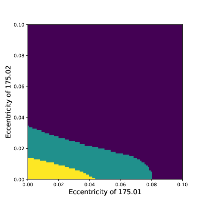
Inspired by the closely-spaced multiplanet systems discovered by Kepler (Muirhead et al., 2015) and other surveys (e.g. Gillon et al. 2017), we also explored the possibility of a fourth, non-transiting planet having a dynamically-stable orbit in-between L 98-59 c and L 98-59 d such that the four planets would form a near-resonant chain of 5:8:12:16 period commensurability similar to e.g. TRAPPIST-1 (Gillon et al. 2017). As an example, we tested a planet with a mass of ${\rm 2.5~{}M_{\oplus}}$ and a 5.7-day orbital period ( ${\rm\approx 1.55}$ and ${\rm\approx 0.77}$ times the period of L 98-59 c and L 98-59 d respectively), again for two cases of (a) initially circular orbits and (b) initially eccentric orbits with $e=0.1$ . For simplicity, we only used the best-fit masses for the three planet candidates. The system is dynamically stable in case (a) for the duration of the integrations (Figure 20, upper panel), and becomes unstable within a few thousand orbits of the outer planet for case (b). Thus such a hypothetical planet is potentially possible if on a circular orbit. Overall, while a comprehensive dynamical analysis for the presence of additional planets is beyond the scope of this work, we will continuously monitor the system as data from future TESS sectors become available.

3.2.2 Transit Timing Variations

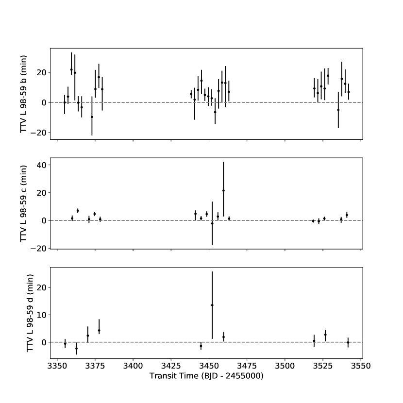
If detected, deviations in the times of transits from a linear ephemeris can be a powerful method to constrain the masses and orbital eccentricities of planets in multiplanet systems (e.g. Agol et al. 2005). We measured transit times for each individual transit using two different methods. First, we folded the transits on a linear ephemeris, fitting a transit model using the models of Mandel & Agol (2002). Next, we measured the time of each individual transit by, for each transit, sliding this model across a grid of potential transit midpoints with a time resolution of one second, and measuring the likelihood of each transit fit at each grid point. We then found the maximum likelihood transit time and a 68% confidence interval on the same. The ability to measure TTV signals depends sensitively on our ability to measure precise transit times. For L 98-59 b, the scatter in measured transit times, suggestive of the ultimate transit timing precision we measure, is 5.1 minutes. For L 98-59 b, this is 2.1 minutes; and for L 98-59 d, 1.2 minutes. Our analysis showed that a linear ephemeris is sufficient to reproduce the transit times of the three planet candidates detected in Sector 2. We found no evidence for transit timing variations (TTVs), and no further constraints can be placed on the parameters of the system beyond those already provided by dynamical stability considerations. Given that L 98-59 will be observed in 7 of the 13 sectors that comprise the first year of the TESS mission (Mukai & Barclay, 2017) (Sectors 2, 5, 8, 9, 10, 11, and 12), here we examine how continued TESS observations would affect the transit timing analysis of the system.

Specifically, we simulated continued observations following the nominal TESS schedule, assuming a linear ephemeris for future transits and that every planned sector will be observed as scheduled. We then used the TTVFast package (Deck et al., 2014) to calculate predicted transit times for the three planets in various orbital configurations consistent with the current data and examine what can be ruled out by the data by the end of the mission.

The two outer planets (L 98-59 c and d) are close to first-order period commensurability (period ratio of 2.02) whereas the inner planet is not near a first-order resonance with either of the other planets (1.64 period ratio between L 98-59 b and L 98-59 c, and 3.31 period ratio between L 98-59 b and L 98-59 d). Thus the expected TTV signal for the former planet pair is stronger compared to that for the latter planet pair. Indeed, even for eccentricities of $\sim 0.1$ , the expected TTV amplitude for the innermost planet is $\sim 90$ seconds, notably smaller than the observed precision on the measured times of transit. To evaluate the potential for measuring TTVs for the outer two planets, we performed numerical simulations of the system for the first year of the TESS mission (using TTVFast), thus covering all sectors it will be observed in. We allowed the planet eccentricities to vary, and assumed the maximum likelihood masses listed in Section 3.1. Adopting a transit-timing precision of 1-2 minutes, we found that significant TTVs could be detected if the eccentricities of the outer two planets were larger than $\sim 0.03$ (as shown in Figure 21).

Overall, as multiplanet systems typically have orbital eccentricities of a few percent (Hadden & Lithwick, 2016), it is unlikely that TESS will reveal timing variations for this system during its primary mission; doing so would suggest either anomalously large eccentricities (which are unlikely based on dynamical stability consideration) or significantly larger planet masses/densities in this system relative to planets with similar radii in other systems.

To explore TTVs using an alternative software framework, we also used the TTV2Fast2Furious package (Hadden et al., 2018) to project the expected TTV signals of the planets through Sector 12, again adopting the forecaster masses and, for simplicity, assuming circular orbits. Similar to the TTVFast analysis described above, our results show that it is unlikely TTVs are measurable for this system during the TESS prime mission — the maximum TTV amplitudes are $0.09$ minutes for L 98-59 b, $0.17$ minutes for L 98-59 c, and $0.56$ minutes for L 98-59 d (see Figure 22).

Following the approach described in Hadden et al. (2018), we also used TTV2Fast2Furious to project the precision of mass constraints derived from future TESS transit timing measurements. Planet mass constraints derived from TTVs depend on the precision of transit time measurements and we adopt the measured scatter in the transit time measurements taken through Sector 2, $\sigma_{t_{L98-59c}}$ = 2.1 minutes, and $\sigma_{t_{L98-59d}}$ = 1.2 minutes. The planets’ masses are expected to be constrained with precisions $\sigma_{m,L98-59c}=13.1\,{\rm M}_{\oplus}$ and $\sigma_{m,L98-59d}=5\,{\rm M}_{\oplus}$ with transit timing data through Sector 12. ¹¹¹¹11If the planets are restricted to circular orbits in the TTV model, e.g., under the assumption that eccentricities are damped away by tidal dissipation, the mass-eccentricity degeneracy (Lithwick et al., 2012) is removed and the measured TTV signals therefore place tighter constraints on the planet masses. In particular, if the TTV model is restricted to circular orbits, the mass measurement precisions of $\sigma_{m,L98-59c}=3.4M_{\oplus}$ and $\sigma_{m,L98-59d}=2.1M_{\oplus}$ are projected.

With three sectors of data available for this system at the time of writing (Sectors 2, 5, and 8), there is at present no evidence for TTVs. In line with the predictions of the previous paragraph, there is no significant mass constraint beyond what is given from plausible compositions of terrestrial planets. We use TTVFast to compare maximum-likelihood dynamical models of the orbits of the planets, assuming the masses listed in Section 3.1. We also repeat this procedure holding the masses fixed at four times this nominal value, which would imply a density of approximately 20 g/cc. In both scenarios, there is a dynamical model which fits the observed transits.

3.3 Potential for Atmospheric Characterization

Owing to the small, bright host star the three planets of the L 98-59 system are promising targets for follow-up atmosphere characterization. The planets’ small radii suggest that it is unlikely that they retain hydrogen-rich atmospheres (Rogers, 2015; Fulton et al., 2017), but secondary atmospheres could form from volcanic outgassing and/or delivery of volatiles from comets.

To investigate the feasibility of atmosphere studies for the L 98-59 planets, we compared the expected signal-to-noise of atmospheric features to that of GJ 1132b, another small planet around a nearby M-dwarf (Berta-Thompson et al., 2015). Morley et al. (2017) found that a CO₂-dominated atmosphere could be detected for GJ 1132 with a modest number of JWST transits or eclipses (11 transits with NIRSpec/G235M or 2 eclipses with MIRI/LRS). To scale these estimates for L 98-59, we used the transmission and emission spectroscopy metrics from Kempton et al. (2018), which calculate expected signal-to-noise for atmospheric features based on planet and star properties. We scaled the signal relative to each planet’s transit/eclipse duration, estimated the brightness of the star based on its K-band magnitude, and assumed zero noise floor. We found that L 98-59 b, L 98-59 c and L 98-59 d have Transmission Spectroscopy Metric (TSM) values of 0.8, 1.4, and 1.0 that of GJ 1132b and Emission Spectroscopy Metric (ESM) values of 0.3, 0.4, and 0.7 respectively (Kempton et al., 2018). This implies that features in the transmission spectrum could be detected with 16, 6, or 11 transits, or 24, 13, or 4 eclipses for L 98-59 b, L 98-59 c and L 98-59 d. Provided that JWST observations reach the photon limit for stars as bright as L 98-59, this system is an exciting opportunity for studying comparative planetology of terrestrial exoplanet atmospheres.

3.4 Planets in the Venus Zone

It is worth noting the possibility that the planets in the system are analogs to Venus in terms of their atmospheric evolution. Venus shares several characteristics with Earth including its relative composition, size, and mass. Although Venus may have previously had temperate surface conditions (Way et al., 2016), Venus eventually diverged significantly from the habitable pathway of Earth and transitioned into a runaway greenhouse state. The planet now has a high pressure, high temperature, and a carbon dioxide dominated atmosphere. In our study of exoplanets and the search for life, it is vitally important that we understand why Earth is habitable and Venus is not (Kane et al., 2014). There is a need to discover planets that may have evolved into a post-runaway greenhouse state so that we can target their atmospheres for characterization with future facilities, such as JWST (Ehrenreich et al., 2012). However, most of the potential Venus analog candidates hitherto discovered orbit relatively faint stars (Barclay et al., 2013; Kane et al., 2013; Angelo et al., 2017; Kane et al., 2018).

The L 98-59 planets receive significantly more energy than the Earth receives from the Sun (a factor of between 4–22 more than Earth’s insolation) and fall into the region that Kane et al. (2014) dubbed the Venus Zone. This is a region where the atmosphere of a planet like Earth would likely have been forced into a runaway greenhouse, producing conditions similar to those found on Venus. The range of incident fluxes within the Venus Zone corresponds to insolations of between 1–25 times that received by the Earth. Planets in the Venus Zone that can be spectroscopically characterized will become increasingly important in the realm of comparative planetology that aims to characterize the conditions for planetary habitability. In that respect, and considering the potential for atmospheric characterization discussed in Section 3.3, L 98-59 could become a benchmark system.

4 Conclusions

We presented the discovery of a system of three transiting, terrestrial-size planets orbiting L 98-59 (TESS Object of Interest TOI-175). The host star is a bright M3 dwarf (K = 7.1) at a distance of 10.6 pc, with ${\rm M_{*}=0.313\pm 0.014M_{\odot}}$ , ${\rm R_{*}=0.312\pm 0.014R_{\odot}}$ , and ${\rm T_{eff}=3367\pm 150K}$ . TFOP-led follow-up observations found no evidence of binarity or significant stellar activity. To thoroughly vet the transit signals detected in the TESS data, we used the software package DAVE. Our analysis ruled out significant secondary eclipses, odd-even differences or photocenter shifts during transits, verifying their planetary nature. Using lightkurve, we also discovered that the nearby field star 2MASS 08181825-6818430, inside the TESS aperture of L 98-59, is an eclipsing binary system with an orbital period of ${\sim 10.43}$ days, manifesting both primary and secondary eclipses. Utilizing Gaia data we confirmed that the eclipsing binary is a background object (likely a red giant) not associated with L 98-59. This battery of tests highlights the importance of comprehensive analysis of all sources inside the TESS aperture.

The planets range in size from slightly smaller to slightly bigger than Earth, with radii of ${\rm 0.8\pm 0.05R_{\oplus}}$ , ${\rm 1.35\pm 0.07R_{\oplus}}$ , and ${\rm 1.59\pm 0.23R_{\oplus}}$ from inner to outer respectively. The planetary system is quite compact, with orbital periods of ${\rm 2.25~{}days}$ , ${\rm 3.69~{}days}$ , and ${\rm 7.45~{}days}$ respectively. We estimated their masses using the forecast package for probabilistic mass forecasting, confirmed the dynamical stability of the system for circular orbits, and showed that there are no significant transit-timing variations.

TESS will continue observing the system in upcoming sectors (9, 10, 11, 12), and it is also likely that the system will be observed during a TESS Extended Mission. These observations will allow for refinement of the known planet parameters, searches for additional planets, further investigations of the dynamics of the system, as well as long-term monitoring of the host star activity.

We thank the referee for the insightful comments that helped us improve this manuscript. This manuscript includes data collected by the TESS mission, which are publicly available from the Mikulski Archive for Space Telescopes (MAST). Funding for the TESS mission is provided by NASA’s Science Mission directorate. We acknowledge the use of TESS Alerts data, as provided by the TESS Science Office. We acknowledge the use of public TESS Alert data from pipelines at the TESS Science Office and at the TESS Science Processing Operations Center. This research has made use of the Exoplanet Follow-up Observation Program website, which is operated by the California Institute of Technology, under contract with the National Aeronautics and Space Administration under the Exoplanet Exploration Program. JGW is supported by a grant from the John Templeton Foundation. Acquisition of the CHIRON data and the first epoch of DSSI data was made possible by a grant from the John Templeton Foundation. The opinions expressed in this publication are those of the authors and do not necessarily reflect the views of the John Templeton Foundation. We thank Leonardo Paredes, Hodari James, Rodrigo Hinojosa, and Todd Henry for their work in gathering and processing the CHIRON data, as well as for the management of CTIO / SMARTS 1.5m telescope. We are also grateful to the observer support staff at CTIO, at ESO/VLT (for program number 0102.C-0503(A)), and Gemini (for program number GS-2018B-LP-101). This work has made use of data from the European Space Agency (ESA) mission Gaia (https://www.cosmos.esa.int/gaia), processed by the Gaia Data Processing and Analysis Consortium (DPAC, https://www.cosmos.esa.int/web/gaia/dpac/consortium). Funding for the DPAC has been provided by national institutions, in particular the institutions participating in the Gaia Multilateral Agreement. This research made use of observations from the LCOGT network, and the AAVSO Photometric All-Sky Survey (APASS), funded by the Robert Martin Ayers Sciences Fund and NSF AST-1412587. The research leading to these results has received funding from the European Research Council under the European Union’s Seventh Framework Programme (FP/2007-2013) ERC Grant Agreement n

\arcdeg

336480, and from the ARC grant for Concerted Research Actions, financed by the Wallonia-Brussels Federation. M.G. and E.J. are FNRS Senior Research Associates. Work by B.T.M. was performed in part under contract with the Jet Propulsion Laboratory (JPL) funded by NASA through the Sagan Fellowship Program executed by the NASA Exoplanet Science Institute. This work is partly supported by JSPS KAKENHI Grant Numbers JP18H01265 and 18H05439, and JST PRESTO Grant Number JPMJPR1775. KH acknowledges support from STFC grant ST/R000824/1.

References

Angelo et al. (2017) Angelo, I., Rowe, J. F., Howell, S. B., et al. 2017, AJ, 153, 162
Anglada-Escudé et al. (2016) Anglada-Escudé, G., Amado, P. J., Barnes, J., et al. 2016, Nature, 536, 437
Astropy Collaboration et al. (2013) Astropy Collaboration, Robitaille, T. P., Tollerud, E. J., et al. 2013, A&A, 558, A33
Astropy Collaboration et al. (2018) Astropy Collaboration, Price-Whelan, A. M., Sipőcz, B. M., et al. 2018, AJ, 156, 123
Baraffe et al. (2003) Baraffe, I., Chabrier, G., Barman, T. S., Allard, F., & Hauschildt, P. H. 2003, A&A, 402, 701
Barclay et al. (2018) Barclay, T., Pepper, J., & Quintana, E. V. 2018, ApJS, 239, 2
Barclay et al. (2015) Barclay, T., Quintana, E. V., Adams, F. C., et al. 2015, ApJ, 809, 7
Barclay et al. (2013) Barclay, T., Burke, C. J., Howell, S. B., et al. 2013, ApJ, 768, 101
Benedict et al. (2016) Benedict, G. F., Henry, T. J., Franz, O. G., et al. 2016, AJ, 152, 141
Berta-Thompson et al. (2015) Berta-Thompson, Z. K., Irwin, J., Charbonneau, D., et al. 2015, Nature, 527, 204
Boyajian et al. (2012) Boyajian, T. S., von Braun, K., van Belle, G., et al. 2012, ApJ, 757, 112
Brown et al. (2013) Brown, T. M., Baliber, N., Bianco, F. B., et al. 2013, Publications of the Astronomical Society of the Pacific, 125, 1031
Bryson et al. (2013) Bryson, S. T., Jenkins, J. M., Gilliland, R. L., et al. 2013, Publications of the Astronomical Society of the Pacific, 125, 889
Burdanov et al. (2018) Burdanov, A., Delrez, L., Gillon, M., & Jehin, E. 2018, SPECULOOS Exoplanet Search and Its Prototype on TRAPPIST, 130
Charalambous et al. (2018) Charalambous, C., Martí, J. G., Beaugé, C., & Ramos, X. S. 2018, MNRAS, 477, 1414
Chen & Kipping (2017) Chen, J., & Kipping, D. 2017, ApJ, 834, 17
Ciardi et al. (2015) Ciardi, D. R., Beichman, C. A., Horch, E. P., & Howell, S. B. 2015, ApJ, 805, 16
Collins et al. (2017) Collins, K. A., Kielkopf, J. F., Stassun, K. G., & Hessman, F. V. 2017, AJ, 153, 77
Cutri et al. (2013) Cutri, R. M., Wright, E. L., Conrow, T., et al. 2013, Explanatory Supplement to the AllWISE Data Release Products, Tech. rep.
Deck et al. (2014) Deck, K. M., Agol, E., Holman, M. J., & Nesvorný, D. 2014, ApJ, 787, 132
Delrez et al. (2018) Delrez, L., Gillon, M., Queloz, D., et al. 2018, in Society of Photo-Optical Instrumentation Engineers (SPIE) Conference Series, Vol. 10700, Ground-based and Airborne Telescopes VII, 107001I
Deming et al. (2015) Deming, D., Knutson, H., Kammer, J., et al. 2015, ApJ, 805, 132
Dittmann et al. (2017) Dittmann, J. A., Irwin, J. M., Charbonneau, D., et al. 2017, Nature, 544, 333
Dragomir et al. (2018) Dragomir, D., Teske, J., Gunther, M. N., et al. 2018, arXiv e-prints, arXiv:1901.00051
Ehrenreich et al. (2012) Ehrenreich, D., Vidal-Madjar, A., Widemann, T., et al. 2012, A&A, 537, L2
Fabrycky et al. (2014) Fabrycky, D. C., Lissauer, J. J., Ragozzine, D., et al. 2014, ApJ, 790, 146
Feinstein et al. (2019) Feinstein, A. D., Schlieder, J. E., Livingston, J. H., et al. 2019, AJ, 157, 40
Foreman-Mackey (2018) Foreman-Mackey, D. 2018, exoplanet v0.1.3, , , doi:10.5281/zenodo.2536576
Foreman-Mackey (2018) Foreman-Mackey, D. 2018, Research Notes of the American Astronomical Society, 2, 31
Foreman-Mackey et al. (2017) Foreman-Mackey, D., Agol, E., Ambikasaran, S., & Angus, R. 2017, AJ, 154, 220
Foreman-Mackey et al. (2013) Foreman-Mackey, D., Hogg, D. W., Lang, D., & Goodman, J. 2013, PASP, 125, 306
Fulton et al. (2017) Fulton, B. J., Petigura, E. A., Howard, A. W., et al. 2017, AJ, 154, 109
Furlan & Howell (2017) Furlan, E., & Howell, S. B. 2017, AJ, 154, 66
Gaia Collaboration et al. (2018) Gaia Collaboration, Brown, A. G. A., Vallenari, A., et al. 2018, A&A, 616, A1
Gaidos et al. (2014) Gaidos, E., Mann, A. W., Lépine, S., et al. 2014, MNRAS, 443, 2561
Gandolfi et al. (2018) Gandolfi, D., Barragán, O., Livingston, J. H., et al. 2018, A&A, 619, L10
Gillon et al. (2013) Gillon, M., Anderson, D. R., Collier-Cameron, A., et al. 2013, A&A, 552, A82
Gillon et al. (2017) Gillon, M., Triaud, A. H. M. J., Demory, B.-O., et al. 2017, Nature, 542, 456
Hadden et al. (2018) Hadden, S., Barclay, T., Payne, M. J., & Holman, M. J. 2018, arXiv e-prints, arXiv:1811.01970
Hadden & Lithwick (2014) Hadden, S., & Lithwick, Y. 2014, ApJ, 787, 80
Hadden & Lithwick (2016) —. 2016, ApJ, 828, 44
Hauschildt et al. (1999) Hauschildt, P. H., Allard, F., & Baron, E. 1999, ApJ, 512, 377
Henden et al. (2016) Henden, A. A., Templeton, M., Terrell, D., et al. 2016, VizieR Online Data Catalog, 2336
Hoffman & Gelman (2014) Hoffman, M. D., & Gelman, A. 2014, Journal of Machine Learning Research, 15, 1593
Horch et al. (2011) Horch, E. P., van Altena, W. F., Howell, S. B., Sherry, W. H., & Ciardi, D. R. 2011, The Astronomical Journal, 141, 180
Huang et al. (2018a) Huang, C. X., Shporer, A., Dragomir, D., et al. 2018a, arXiv e-prints, arXiv:1807.11129
Huang et al. (2018b) Huang, C. X., Burt, J., Vanderburg, A., et al. 2018b, ApJ, 868, L39
Hunter (2007) Hunter, J. D. 2007, Computing In Science & Engineering, 9, 90
Irwin et al. (2015) Irwin, J. M., Berta-Thompson, Z. K., Charbonneau, D., et al. 2015, in Cambridge Workshop on Cool Stars, Stellar Systems, and the Sun, Vol. 18, 18th Cambridge Workshop on Cool Stars, Stellar Systems, and the Sun, 767–772
Jenkins et al. (2017) Jenkins, J. M., Seader, S., & Burke, C. J. 2017, Kepler Data Processing Handbook: A Statistical Bootstrap Test, Tech. rep.
Jenkins et al. (2016) Jenkins, J. M., Twicken, J. D., McCauliff, S., et al. 2016, in Proc. SPIE, Vol. 9913, Software and Cyberinfrastructure for Astronomy IV, 99133E
Jensen (2013) Jensen, E. 2013, Tapir: A web interface for transit/eclipse observability, Astrophysics Source Code Library, , , ascl:1306.007
Kane et al. (2013) Kane, S. R., Barclay, T., & Gelino, D. M. 2013, ApJ, 770, L20
Kane et al. (2018) Kane, S. R., Ceja, A. Y., Way, M. J., & Quintana, E. V. 2018, ApJ, 869, 46
Kane et al. (2014) Kane, S. R., Kopparapu, R. K., & Domagal-Goldman, S. D. 2014, ApJ, 794, L5
Kempton et al. (2018) Kempton, E. M.-R., Bean, J. L., Louie, D. R., et al. 2018, PASP, 130, 114401
Kipping (2013a) Kipping, D. M. 2013a, MNRAS, 435, 2152
Kipping (2013b) —. 2013b, MNRAS, 434, L51
Kluyver et al. (2016) Kluyver, T., Ragan-Kelley, B., Pérez, F., et al. 2016, in Positioning and Power in Academic Publishing: Players, Agents and Agendas, ed. F. Loizides & B. Scmidt (IOS Press), 87–90
Kostov et al. (2019) Kostov, V. B., Mullally, S. E., Quintana, E. V., et al. 2019, arXiv e-prints, arXiv:1901.07459
Li et al. (2019) Li, J., Tenenbaum, P., Twicken, J. D., et al. 2019, PASP, 131, 024506
Lightkurve Collaboration et al. (2018) Lightkurve Collaboration, Cardoso, J. V. d. M., Hedges, C., et al. 2018, Lightkurve: Kepler and TESS time series analysis in Python, , , ascl:1812.013
Lissauer et al. (2011) Lissauer, J. J., Ragozzine, D., Fabrycky, D. C., et al. 2011, ApJS, 197, 8
Lissauer et al. (2012) Lissauer, J. J., Marcy, G. W., Rowe, J. F., et al. 2012, ApJ, 750, 112
Lithwick et al. (2012) Lithwick, Y., Xie, J., & Wu, Y. 2012, ApJ, 761, 122
Livingston et al. (2018) Livingston, J. H., Crossfield, I. J. M., Petigura, E. A., et al. 2018, AJ, 156, 277
Louie et al. (2018) Louie, D. R., Deming, D., Albert, L., et al. 2018, Publications of the Astronomical Society of the Pacific, 130, 044401
Luger et al. (2018) Luger, R., Agol, E., Foreman-Mackey, D., et al. 2018, ArXiv e-prints, 1810.06559
Luger et al. (2016) Luger, R., Agol, E., Kruse, E., et al. 2016, AJ, 152, 100
Mandel & Agol (2002) Mandel, K., & Agol, E. 2002, ApJ, 580, L171
Mann et al. (2015) Mann, A. W., Feiden, G. A., Gaidos, E., Boyajian, T., & von Braun, K. 2015, ApJ, 804, 64
Mayor et al. (2009) Mayor, M., Bonfils, X., Forveille, T., et al. 2009, A&A, 507, 487
McKinney (2010) McKinney, W. 2010, in Proceedings of the 9th Python in Science Conference, ed. S. van der Walt & J. Millman, 51 – 56
Ment et al. (2018) Ment, K., Dittmann, J. A., Astudillo-Defru, N., et al. 2018, ArXiv e-prints, arXiv:1808.00485
Morley et al. (2017) Morley, C. V., Kreidberg, L., Rustamkulov, Z., Robinson, T., & Fortney, J. J. 2017, ApJ, 850, 121
Morton et al. (2016) Morton, T. D., Bryson, S. T., Coughlin, J. L., et al. 2016, ApJ, 822, 86
Muirhead et al. (2018) Muirhead, P. S., Dressing, C. D., Mann, A. W., et al. 2018, AJ, 155, 180
Muirhead et al. (2015) Muirhead, P. S., Mann, A. W., Vanderburg, A., et al. 2015, ApJ, 801, 18
Mukai & Barclay (2017) Mukai, K., & Barclay, T. 2017, tvguide: A tool for determining whether stars and galaxies are observable by TESS., v.1.0.1, Zenodo, doi:10.5281/zenodo.823357
Newton et al. (2015) Newton, E. R., Charbonneau, D., Irwin, J., & Mann, A. W. 2015, ApJ, 800, 85
Nielsen et al. (2018) Nielsen, L. D., Bouchy, F., Turner, O., et al. 2018, arXiv e-prints, arXiv:1811.01882
Oliphant (2007) Oliphant, T. E. 2007, Computing in Science Engineering, 9, 10
Pecaut & Mamajek (2013) Pecaut, M. J., & Mamajek, E. E. 2013, ApJS, 208, 9
Perez & Granger (2007) Perez, F., & Granger, B. E. 2007, Computing in Science Engineering, 9, 21
Quinn et al. (2019) Quinn, S. N., Becker, J. C., Rodriguez, J. E., et al. 2019, arXiv e-prints, arXiv:1901.09092
Quintana et al. (2014) Quintana, E. V., Barclay, T., Raymond, S. N., et al. 2014, Science, 344, 277
Rein & Spiegel (2015) Rein, H., & Spiegel, D. S. 2015, MNRAS, 446, 1424
Ricker et al. (2015) Ricker, G. R., Winn, J. N., Vanderspek, R., et al. 2015, Journal of Astronomical Telescopes, Instruments, and Systems, 1, 014003
Rodriguez et al. (2019) Rodriguez, J. E., Quinn, S. N., Huang, C. X., et al. 2019, arXiv e-prints, arXiv:1901.09950
Rogers (2015) Rogers, L. A. 2015, ApJ, 801, 41
Rowe et al. (2014) Rowe, J. F., Bryson, S. T., Marcy, G. W., et al. 2014, ApJ, 784, 45
Salvatier et al. (2016) Salvatier, J., Wiecki, T. V., & Fonnesbeck, C. 2016, PeerJ Computer Science, 2, e55
Shporer et al. (2018) Shporer, A., Wong, I., Huang, C. X., et al. 2018, arXiv e-prints, arXiv:1811.06020
Simcoe et al. (2008) Simcoe, R. A., Burgasser, A. J., Bernstein, R. A., et al. 2008, in Society of Photo-Optical Instrumentation Engineers (SPIE) Conference Series, Vol. 7014, Ground-based and Airborne Instrumentation for Astronomy II, 70140U
Skrutskie et al. (2006) Skrutskie, M. F., Cutri, R. M., Stiening, R., et al. 2006, AJ, 131, 1163
Smith et al. (2012) Smith, J. C., Stumpe, M. C., Van Cleve, J. E., et al. 2012, PASP, 124, 1000
Stassun et al. (2017) Stassun, K. G., Collins, K. A., & Gaudi, B. S. 2017, AJ, 153, 136
Stassun & Torres (2016) Stassun, K. G., & Torres, G. 2016, AJ, 152, 180
Stassun & Torres (2018) —. 2018, ApJ, 862, 61
Stassun et al. (2018) Stassun, K. G., Oelkers, R. J., Pepper, J., et al. 2018, AJ, 156, 102
Stumpe et al. (2014) Stumpe, M. C., Smith, J. C., Catanzarite, J. H., et al. 2014, PASP, 126, 100
Theano Development Team (2016) Theano Development Team. 2016, arXiv e-prints, abs/1605.02688
Tokovinin et al. (2013) Tokovinin, A., Fischer, D. A., Bonati, M., et al. 2013, PASP, 125, 1336
Twicken et al. (2018) Twicken, J. D., Catanzarite, J. H., Clarke, B. D., et al. 2018, PASP, 130, 064502
van der Walt et al. (2011) van der Walt, S., Colbert, S. C., & Varoquaux, G. 2011, Computing in Science Engineering, 13, 22
Vanderspek et al. (2018) Vanderspek, R., Huang, C. X., Vanderburg, A., et al. 2018, arXiv e-prints, arXiv:1809.07242
Wang et al. (2018) Wang, S., Jones, M., Shporer, A., et al. 2018, arXiv e-prints, arXiv:1810.02341
Way et al. (2016) Way, M. J., Del Genio, A. D., Kiang, N. Y., et al. 2016, Geophys. Res. Lett., 43, 8376
Welsh et al. (2011) Welsh, W. F., Orosz, J. A., Aerts, C., et al. 2011, ApJS, 197, 4
Winters et al. (2015) Winters, J. G., Henry, T. J., Lurie, J. C., et al. 2015, AJ, 149, 5
Winters et al. (2018) Winters, J. G., Irwin, J., Newton, E. R., et al. 2018, AJ, 155, 125
Winters et al. (2019) Winters, J. G., Henry, T. J., Jao, W.-C., et al. 2019, arXiv e-prints, arXiv:1901.06364
Zacharias et al. (2017) Zacharias, N., Finch, C., & Frouard, J. 2017, AJ, 153, 166
Ziegler et al. (2018) Ziegler, C., Law, N. M., Baranec, C., et al. 2018, AJ, 155, 161