WASP-180Ab: Doppler tomography of an hot Jupiter orbiting the primary star in a visual binary

Abstract

We report the discovery and characterisation of WASP-180Ab, a hot Jupiter confirmed by the detection of its Doppler shadow and by measuring its mass using radial velocities. We find the 0.9 $\pm$ 0.1 $M_{\rm Jup}$, 1.24 $\pm$ 0.04 $R_{\rm Jup}$ planet to be in a misaligned, retrograde orbit around an F7 star with $T_{\rm eff}$ = 6500 K and a moderate rotation speed of $v\sin i_{\star}$ = 19.9 km s^-1. The host star is the primary of a $V$ = 10.7 binary, where a secondary separated by $\sim$5^′′ ($\sim$1200 AU) contributes $\sim$ 30% of the light. WASP-180Ab therefore adds to a small sample of transiting hot Jupiters known in binary systems. A 4.6-day modulation seen in the WASP data is likely to be the rotational modulation of the companion star, WASP-180B.

1 Introduction

In the age of high resolution spectrographs, the possibilities for detailed characterisation of exoplanets are expanding. We are able to map the motion of a hot Jupiter across the disc of its host star as it transits, via a method called Doppler tomography. This method consists of the direct detection of distortions to stellar line profiles that occur due to the occultation of a portion of the stellar disc by a smaller orbiting body, a phenomenon called the Rossiter-McLaughlin (RM) effect (e.g. Collier Cameron et al., 2010; Siverd et al., 2018; Temple et al., 2019). In mapping the motion of this distortion as a function of phase, it is possible to determine the current projected spin-orbit misalignment angle, $\lambda$, measured as the apparent angle between the stellar rotation axis and the normal to the orbital plane of the planet. Knowledge of $\lambda$ gives insight to the dynamical history of the system. Doppler tomography is especially suited to hotter targets which elude radial velocity characterisation due to a lack of spectral lines. It can also reveal the effects of internal stellar motions on the surface of a star, such as differential rotation and convection (Cegla et al., 2016b) and stellar pulsations (see, e.g. Temple et al., 2017).

In this work we present a newly discovered hot Jupiter, WASP-180Ab, transiting the primary star of a visual binary in a misaligned, retrograde orbit.

This discovery may be in line with theories surrounding Lidov-Kozai oscillations being responsible for the high obliquities seen in some hot-Jupiter systems (e.g. Anderson et al., 2016; Storch et al., 2017). It has long been theorized that a distant stellar companion can induce such oscillations in a Jupiter’s orbit, leading to high-eccentricity migration of the planet which produces a misaligned, short-period orbit. This would then be followed by realignment of the host star with the planet’s orbit via tidal dissipation, an effect that would be less efficient for stellar hosts lacking convective envelopes, and thus this theory is consistent with the observed tendency of systems with stars hotter than $\sim$ 6250 K being more likely to have planetary orbits which are misaligned with respect to the stellar rotation axis (Winn et al., 2010; Albrecht et al., 2012).

Through the works of Ngo et al. (2015); Piskorz et al. (2015); Ngo et al. (2016); Evans et al. (2018), for example, we now know that a large portion of the known planet population consists of systems containing lower mass stellar companions, with Ngo et al. (2016) concluding that 47% $\pm$ 7% of hot Jupiters have stellar companions at separations of 50–2000 AU. Meanwhile, Evans et al. (2018) show that there is a dearth of planets in wide binary systems with stars of similar mass. It should be noted, however, that this finding is at least partially a selection bias: in systems with stars of similar mass and thus brightness, as in the case of WASP-180, the light from the planet hosting star is significantly diluted in the light of the other star, reducing the apparent transit depth and making detection via the transit method more difficult. Now, WASP-180Ab adds to a small group of known hot Jupiters in near-equal mass stellar binaries.

2 Data and Observations

WASP-180 is a known binary, listed as WDS 08136-0159 in the Washington Double Star Catalogue (Mason et al., 2001), with the two stars having Gaia magnitudes of 10.9 and 11.8. Gaia DR2 confirms the two stars to have the same parallax and proper motions, and we calculate the angular separation to be 4.854^′′ (Gaia Collaboration et al., 2016, 2018). This separation is sufficient to avoid contamination in high-resolution spectroscopic observations of the system.

We observed WASP-180A from November 2009 to March 2012 using the SuperWASP-North telescope (Pollacco et al., 2006) located at the Roque de los Muchachos Observatory in La Palma, as well as the WASP-South telescope (Hellier et al., 2011) located at the South African Astronomical Observatory (SAAO). The data contains light from both WASP-180A and WASP-180B.

Upon detecting a 3.4-d transit-like signal in the WASP data we obtained focused photometry with TRAPPIST-South (Jehin et al., 2011), resolving the two stars. These data were sufficient to show that the transit is of the brighter of the two stars, WASP-180A, but were otherwise of low quality and so we exclude the lightcurve from further analysis.

We proceeded to obtain radial velocity (RV) measurements with the Euler/CORALIE (Queloz et al., 2001) spectrograph. WASP-180A is a fast rotating F star with broad lines giving large RV errors, so the CORALIE RVs ruled out a stellar-mass transit mimic, but were not sufficient to give a measurement of the planet’s mass. Thus we attempted Doppler tomography of a transit on the night of 2018 January 5 using the ESO 3.6-m/HARPS spectrograph (Pepe et al., 2002). Due to an auto-guiding issue three of the spectra obtained were of low signal-to-noise and were therefore discarded. Simultaneously during this transit we observed the lightcurve using TRAPPIST-South, using an aperture including both stars.

After tomographic confirmation of the planet we observed further follow-up lightcurves also using apertures including both stars. These were taken with TRAPPIST-North (Barkaoui et al., 2017, 2019) at the Oukaïmden Observatory in Morocco and the SPECULOOS-Callisto telescope (Burdanov et al., 2018) at ESO Paranal Observatory. We also obtained 6 more RVs with HARPS to constrain the planet’s mass. Details of the observations used in this work are provided in Table  1.

The RV measurements corresponding to each of the spectra obtained are listed in Table  2 with the corresponding bisector span (BS) measurements. These were measured from cross-correlation functions (CCFs) computed by cross-correlating the spectra using a mask matching a G2 spectral type, over a wide correlation window covering –320 km s^-1 to 380 km s^-1.

Table 1: Details of the photometric and spectroscopic observations of WASP-180Ab carried out for this work.

Telescope/Instrument	Date	Notes
WASP-North	2009–2011	8329 points
WASP-South	2011–2012	4359 points
TRAPPIST-South	2018 Jan 5	z’. 10s exp.
TRAPPIST-North	2018 Jan 12	z’. 11s exp.
SPECULOOS-Callisto	2018 Jan 22	z’. 8s exp.
ESO 3.6-m/HARPS	2018 Jan 5	21 spectra
		through transit
Euler/CORALIE	2015–2018	9 RVs
ESO 3.6-m/HARPS	2018 Mar	6 RVs

Table 2: RV measurements for WASP-180A taken using the CORALIE and HARPS spectrographs for this work. The values in italics are of low signal-to-noise due to an auto-guiding issue during observation.

BJDTDB	RV	$\sigma$RV	BS	$\sigma$BS
–2,450,000	(km s-1)	(km s-1)	(km s-1)	(km s-1)
CORALIE:
7092.644031	28.96	0.05	–0.18	0.10
7697.849714	28.96	0.06	0.01	0.12
7751.760876	29.02	0.06	–0.29	0.12
8077.824503	28.76	0.04	–0.12	0.08
8079.836204	28.90	0.05	–0.21	0.10
8094.796351	28.65	0.04	–0.00	0.08
8140.848419	28.90	0.06	–0.15	0.12
8212.592949	29.06	0.06	–0.11	0.12
8222.600891	28.95	0.07	–0.16	0.14
HARPS:
8198.604103	29.02	0.02	–0.25	0.04
8199.643111	28.85	0.02	–0.04	0.04
8201.610172	29.01	0.02	–0.07	0.04
8202.589668	29.01	0.02	–0.06	0.04
8203.572959	28.87	0.02	–0.19	0.04
8204.571804	28.91	0.02	–0.01	0.04
HARPS (2018 Jan 05):
8124.596974	28.99	0.02	–0.23	0.04
8124.607854	29.05	0.02	–0.21	0.04
8124.618421	28.98	0.02	–0.17	0.04
8124.629200	28.96	0.02	–0.15	0.04
8124.640806	28.90	0.02	–0.11	0.04
8124.650841	28.76	0.02	0.03	0.04
8124.661525	28.76	0.02	0.22	0.04
8124.672312	28.81	0.02	0.17	0.04
8124.683285	28.91	0.02	–0.12	0.04
8124.693748	29.02	0.02	–0.31	0.04
8124.704420	29.10	0.02	–0.48	0.04
8124.715299	29.20	0.03	–0.75	0.06
8124.725971	29.16	0.03	–0.63	0.06
8124.736434	29.02	0.04	0.10	0.08
8124.746794	29.16	0.04	–0.03	0.08
8124.758090	28.35	0.05	–1.30	0.10
8124.770313	28.91	0.02	–0.18	0.04
8124.780059	28.95	0.02	–0.22	0.04
8124.790510	28.91	0.02	–0.19	0.04
8124.801182	28.88	0.02	–0.22	0.04
8124.812062	28.91	0.03	–0.18	0.06

3 Spectral analysis

We analysed a median-stacked HARPS spectrum created from the 18 HARPS spectra taken on the night of 2018 Jan 5, to obtain stellar parameters. We follow the methods of Doyle et al. (2013) to measure $T_{\rm eff}$ = 6500 $\pm$ 150 K and $\log{g_{*}}$ = 4.5 $\pm$ 0.2 dex. We measure $v\sin i_{\star}$ = 18.3 $\pm$ 1.1 km s^-1 by assuming a microturbulence value of $v_{\rm mic}$ = 1.5 km s^-1 from the calibration of Bruntt et al. (2010) and a macroturbulence value of 5.8 km s^-1 extrapolated from the calibrations of Doyle et al. (2014), which is valid for stars up to 6400 K. We also measure the metallicity as [Fe/H] = 0.09$\pm$0.19, and finally, use the MKCLASS program (Gray & Corbally, 2014) to obtain a spectral type of F7 V.

4 The distant co-moving companion

The average parallax of WASP-180 measured by Gaia DR2 is 3.885 mas and the angular separation is 4.854 ^′′, which indicates a projected binary separation of $\sim$ 1200 AU. This would imply an orbit of $\sim$ 30 000 yrs, which is compatible with the fact that no significant change in separation or position angle is seen in measurements taken over a period of 120 years, as listed in the WDS.

4.1 Correcting for dilution

Our photometry of WASP-180 was all extracted from an aperture including both A and B components. Thus we need to correct the lightcurves for dilution. We deduced correction factors in the different bands of SDSS z and Johnson V, the latter of which was used as an approximation for the WASP data. These are estimated from deducing the effective temperatures of the two stars from available photometry, as follows.

We fitted $T_{\rm eff}$, $\log{g_{*}}$, and [Fe/H] by comparing resolved catalogue photometry to the synthetic photometry of Casagrande & VandenBerg (2014, 2018) which uses the marcs stellar models of Gustafsson et al. (2008). The stars were assumed to have identical [Fe/H]. Interstellar reddening was found to be poorly constrained by the photometry, and was instead fixed at E(B–V) = 0.01, derived from the 3D dust map of Green et al. (2014, 2015), adopting the closest reliable reddening measurements in the map, at approximately 400 pc. The choice of distance does not significantly affect the results, with the full line-of-sight reddening out to 8 kpc being E(B–V) = 0.02 $\pm$ 0.02. Resolved photometry was found in PANSTARRS-1 (grizy Chambers et al., 2016), CMC15 (r’ Niels Bohr Institute et al., 2014), DENIS (IJK Epchtein et al., 1997), and 2MASS (JHK Cutri et al., 2003). The PANSTARRS-1 catalogue does not include uncertainties for the measurements, and so a conservative uncertainty of 0.1 mag was assigned to all measurements in that catalogue.

Stellar parameters were derived by least-squares minimisation to find the minimum $\chi^{2}$, and uncertainties were determined by perturbing each parameter separately until a $\delta\chi^{2}$ of 1 was reached. We found $\log{g_{*}}$ to be poorly constrained by the photometry, with the entire range of the synthetic photometry grids (3.0 $\leq$ $\log{g_{*}}$ $\leq$ 5.0) failing to give $\delta\chi^{2}$ > 1. Temperatures of 6540${}^{+80}_{-30}$ K and 5430${}^{+30}_{-25}$ K were obtained for the A and B components respectively, as well as a joint [Fe/H] value of 0.0${}^{+0.1}_{-0.5}$. The fitting was also repeated four further times, excluding each of the four photometric catalogues (PANSTARRS-1, CMC15, DENIS, 2MASS) in turn. The mean and standard deviation of the parameters from these four additional fits are T_A = 6521 $\pm$ 56 K, T_B = 5425 $\pm$ 17 K, and [Fe/H] = –0.01 $\pm$ 0.01: in good agreement with the full fit, indicating that none of the four photometric surveys is significantly biased. The values of T_A we obtain are consistent with the value of $T_{\rm eff}$ from the spectral analysis (Sec. 3).

Using the stellar parameters from the full fit, and a fixed $\log{g_{*}}$ of 4.5 (consistent with spectral analysis), flux ratios were estimated from the synthetic photometry for the z’ and V bands. The fraction of light contributed by the secondary star was calculated, and thus the light curves corrected for the dilution of the planetary transit. The third light values and stellar flux ratios we obtained are given in Table 3.

Table 3: Third light dilution factors and stellar flux ratios obtained for WASP-180.

Passband	Third Light	Flux Ratio
SDSS z	0.325 $\pm$ 0.007	0.48 $\pm$ 0.01
Johnson V	0.260 $\pm$ 0.006	0.351 $\pm$ 0.008

4.2 IRFM analysis

We use the InfraRed Flux Method (IRFM Blackwell & Shallis, 1977) to derive stellar angular diameters and IR temperatures for WASP-180A and WASP-180B. The IRFM makes use of the insensitivity of stellar surface flux to $T_{\rm eff}$ at IR wavelengths to determine $T_{\rm eff}$ from the ratio of total integrated flux to monochromatic flux, and thus measure the angular diameter of a star. We combine the angular diameters with the Gaia DR2 parallaxes for the two stars, applying the correction to Gaia DR2 parallaxes suggested by Stassun & Torres (2018), to estimate their radii. We calculate $R_{\star\rm,A}$ = 1.17 $\pm$ 0.08$R_{\odot}$ and $R_{\star\rm,B}$ = 1.07 $\pm$ 0.06$R_{\odot}$.

4.3 Rotational modulation search

We perform a search of the WASP photometry following the method of Maxted et al. (2011), looking for rotational modulation or pulsation signals with frequencies of 0–1 cycles day^-1. The data were split into three parts according to the observing season and camera used. We find a signal with an average amplitude of $\sim$ 0.004 mag and an average period of 4.57 $\pm$ 0.05 days. The strongest peak in the first set of data lies at half the modulation period $P_{\rm mod}$. The last set of data contained the clearest signal, and so was given double weight when computing the average. We display the periodograms for each set of data in Fig. 1, and give the individual best-fit amplitudes and periods in Table 4.

Table 4: The results of the rotational modulation search of the WASP photometry of WASP-180. The strongest peak in the periodogram for the first set of data lies at $P_{\rm mod}$/2 (see Fig. 1). The additional peaks around 1–2 days are ascribed to a combination of harmonics of the rotation period and 1-day aliases.

Dates (HJD–	No. pts	Period	Amplitude	False Alarm
2450000)		(days)	(mag)	Probability
5155–5272	3660	2.28	0.004	0.064
5520–5623	3744	4.68	0.003	0.099
5899–6018	3171	4.53	0.004	< 0.001

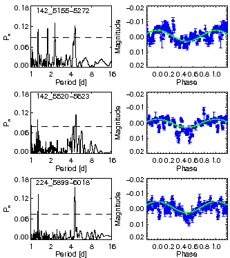
Figure 1: Results of the rotational modulation search of the WASP photometry of WASP-180. The three rows show the periodogram (left) and phase-folded light curve (right) for each chunk of data, displayed in the same order as they are listed in Table 4. The horizontal dashed line in each of the periodograms corresponds to a confidence level of 99%.

Using the measured $v\sin i_{\star}$ from spectral analysis (18.3 $\pm$ 1.1 km s^-1) and the adopted stellar radius from the combined analysis (1.19 $\pm$0.06 R_⊙), we obtain an upper limit on the rotation period of WASP-180A, finding $P_{\rm rot}$ < 3.3 days. This compares with the modulation period of $\sim$ 4.6 days, implying that the signal does not originate from rotational modulation in WASP-180A.

The co-moving companion star WASP-180B contributes $\sim$ 30% of the total flux, and so the true amplitude of the signal if originating from the secondary would be $\sim$ 1%, which is consistent with spot modulation on a fast-rotating later-type star. Gaia DR2 does not find any other close neighbours which may contribute to the total flux. Thus we believe the signal to belong to the visual companion star, which has a temperature of 5430${}^{+30}_{-25}$ K. A rotation period of 4.6 days is fairly rapid for a star of $T_{\rm eff}$ = 5430${}^{+30}_{-25}$ K, which may imply a young age for the system, consistent with our bagemass analysis in Section 6.

5 Combined MCMC analysis

We use a Markov Chain Monte Carlo (MCMC) approach to fit the combined photometric and radial velocity data, as well as investigate the RM effect. We follow methods very similar to Temple et al. (2018, 2019), whereby we conduct both an RM analysis and a tomographic analysis and adopt the better-constrained solution. The RM analysis involves detecting the line-profile distortions as an apparent overall shift in radial velocity measurements (e.g. Triaud, 2017), whereas the tomographic analysis requires one to directly map the motion of the distortion caused by the occulting body across the line profiles as a function of phase (e.g. Brown et al., 2017; Temple et al., 2017).

The code we use is described by Collier Cameron et al. (2007); Pollacco et al. (2008); Collier Cameron et al. (2010). The combined photometric and RV fitting determines the orbital period $P$, the epoch of mid-transit $T_{\rm c}$, the planet-to-star area ratio $(R_{\rm p}/R_{\star})^{2}$, the transit duration $T_{\rm 14}$, the impact parameter $b$, the stellar reflex velocity semi-amplitude $K_{\rm 1}$ and the barycentric system velocity $\gamma$. We use the value of $T_{\rm eff}$ obtained in the dilution correction as input, and interpolate four-parameter limb darkening coefficients from the Claret (2000, 2004) tables in each step using the current value of $T_{\rm eff}$. We use the stellar radius obtained in Sec. 4.2 (1.17 $\pm$ 0.08$R_{\odot}$) as a prior to constrain stellar parameters. In the fit we present we have assumed that the orbit is circular, as one would expect a hot Jupiter to circularise on a timescale shorter than its lifetime (Pont et al., 2011). However, a further fit was carried out to test this assumption, leading to an upper limit of $e$ < 0.27 (95% confidence). We display the photometry and best-fit transit model in Fig. 2.

The RM fit and Doppler tomography give values for $v\sin i_{\star}$, $\lambda$ and the system $\gamma$-velocity. We use the calibrations of Hirano et al. (2011) to fit the RM effect. For Doppler tomography, we assume a Gaussian profile for the perturbation to the stellar-line profiles and fit the intrinsic Full-Width at Half-Maximum (FWHM) of the perturbation, $v_{\rm FWHM}$. Both methods also provide an additional constraint on the impact parameter $b$, although the tomographic method fits this quantity more directly. We estimate the start value for $\gamma$ by fitting a Gaussian profile to the CCFs. We also apply the spectral $v\sin i_{\star}$ as a prior in both fitting modes.

We find that the tomographic method was better able to constrain $v\sin i_{\star}$ and $\lambda$. In the RM fit, the value of $v\sin i_{\star}$ was less constrained, even when using the spectral $v\sin i_{\star}$ as a prior. Thus we adopt the solution to the fit including Doppler tomography. We give the solutions for both methods in Table 5. The RV measurements used in this analysis and the best-fit RV and RM models are displayed in Fig. 3.

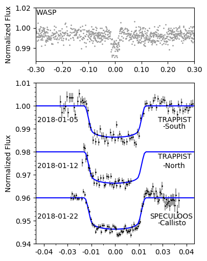
Figure 2: The WASP discovery photometry (top) and follow-up transit lightcurves (bottom) with the best-fitting model shown in blue. (see Section 5). The data for the three follow-up lightcurves, prior to the dilution correction, are available online as supporting material.

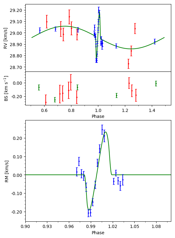
Figure 3: Top: All RV measurements of WASP-180A used in this work together with the best-fit model shown in green. The red points are CORALIE measurements and the blue points are HARPS measurements. Middle: the bisector (BS) measurements corresponding to the RVs in the top panel. Bottom: The RV measurements taken during transit and best-fit RM model.

Figure 4 shows the tomographic dataset used in this analysis. We have subtracted an average of the out-of-transit CCFs in the dataset from each CCF in order to display the residual bump due to the planet transit. The planet signal is strong and clear, moving in a retrograde direction. Due to excluding three of the CCFs (having low signal-to-noise) we are missing the transit egress. We also show the simultaneous photometric observation in Fig. 4 and a residuals plot produced by subtracting the planet model from the tomographic data.

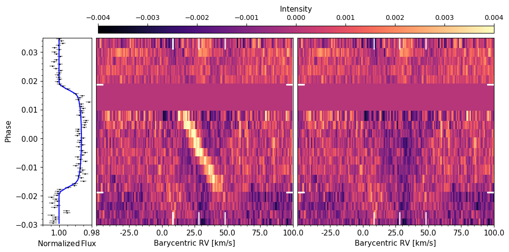
Figure 4: The Doppler tomogram for WASP-180Ab, showing the strong retrograde planet trace (middle) and simultaneous photometric observation alongside (left). The right-hand panel shows the residuals remaining after subtracting the fit to the perturbation due to the planet (see Section 5). The white vertical dashes in the centre and right-hand panels mark the positions of $\gamma$ and $\gamma\,\pm$ $v\sin i_{\star}$  while the white horizontal dashes indicate the times of 1^st and 4${\rm th}$ contacts of the planet.

Table 5: All system parameters obtained for WASP-180 in this work. The quantities marked with * were used as priors in the combined MCMC analysis described in Section 5.

Stellar system
WASP-180A aliases:	1SWASP J081334.15–015857.9		2MASS 08133416–0158579		TIC ID:178367144
WASP-180A Coordinates:	RA = 08h13m34.15s      Dec = –01∘58${}^{{}^{\prime}}$57.9${}^{{}^{\prime\prime}}$ (J2000)
Magnitude measurements:
	WASP-180A		WASP-180B
$B$ (ucac4rpm)	11.221 $\pm$ 0.3		12.732 $\pm$ 0.3
$V$ (ucac4rpm)	10.682 $\pm$ 0.3		12.041 $\pm$ 0.3
$g^{\prime}$ (Pan-STARRS)	10.96 $\pm$ 0.3		12.336 $\pm$ 0.3
$r^{\prime}$ (Pan-STARRS)	10.791 $\pm$ 0.3		11.887 $\pm$ 0.3
$i^{\prime}$ (Pan-STARRS)	10.786 $\pm$ 0.3		11.713 $\pm$ 0.3
$z^{\prime}$ (Pan-STARRS)	10.836 $\pm$ 0.3		11.637 $\pm$ 0.3
$G$ (Gaia DR2)	10.9134 $\pm$ 0.0007		11.7712 $\pm$ 0.0008
$J$ (2MASS)	10.11 $\pm$ 0.05		10.68 $\pm$ 0.03
SED analysis
$T_{\rm eff}$	6540${}^{+80}_{-30}$ K*		5430${}^{+30}_{-25}$ K
$\rm[Fe/H]$	0.0${}^{+0.1}_{-0.5}$		0.0${}^{+0.1}_{-0.5}$
IRFM, distance and proper motions
$T_{\rm eff}$	6530 $\pm$ 190 K		5450 $\pm$ 130 K
$\theta$	0.040 $\pm$ 0.002 mas		0.038 $\pm$ 0.004 mas
Gaia DR2 Proper Motions:
RA	–14.05 $\pm$ 0.09 mas yr-1		–12.7 $\pm$ 0.2 mas yr-1
DEC	–3.17 $\pm$ 0.06 mas yr-1		–2.7 $\pm$ 0.1 mas yr-1
Gaia DR2 Parallax	3.909 $\pm$ 0.052 mas		3.862 $\pm$ 0.073 mas
$R_{\star}$	1.17 $\pm$ 0.08$R_{\odot}$*		1.07 $\pm$ 0.06$R_{\odot}$
Stellar parameters of WASP-180A from spectral analysis:
Parameter	Value		Parameter	Value
(Unit)			(Unit)
$T_{\rm eff}$ (K)	6500 $\pm$ 150		$v\sin i_{\star}$ (km s-1)	18.3 $\pm$ 1.1*
$\log{g_{*}}$	4.5 $\pm$ 0.2		$\rm[Fe/H]$	0.09 $\pm$ 0.19
$v_{\rm mac}$	5.8		Spectral type	F7 V
$v_{\rm mic}$	1.5		-
Parameters from combined analyses:
Parameter	DT Value	RM Value:	Parameter	DT Value	RM Value:
(Unit)	(adopted):		(Unit)	(adopted):
$P$ (d)	3.409264 $\pm$ 0.000001	3.409265 $\pm$ 0.000001	$T_{\rm eff}$ (K)	6600 $\pm$ 200	6600 $\pm$ 100
$T_{\rm c}$ (BJDTDB)	2457763.3150 $\pm$ 0.0001	2457763.3148 $\pm$ 0.0003	[Fe/H]	0.1 $\pm$ 0.2	0.1 $\pm$ 0.2
$T_{\rm 14}$ (d)	0.1299 $\pm$ 0.0004	0.1285 $\pm$ 0.0009	$M_{\rm P}$ ($M_{\rm Jup}$)	0.9 $\pm$ 0.1	0.9 $\pm$ 0.2
$T_{\rm 12}=T_{\rm 34}$ (d)	0.0141 $\pm$ 0.0002	0.0145 $\pm$ 0.0008	$R_{\rm P}$ ($R_{\rm Jup}$)	1.24 $\pm$ 0.04	1.28 $\pm$ 0.09
$R_{\rm P}^{2}$/R${}_{*}^{2}$	0.0123 $\pm$ 0.0002	0.0125 $\pm$ 0.0002	$\log g_{\rm P}$ (cgs)	3.12 $\pm$ 0.05	3.10 $\pm$ 0.06
$b$	0.29 $\pm$ 0.02	0.34 $\pm$ 0.06	$\rho_{\rm P}$ ($\rho_{\rm J}$)	0.46 $\pm$ 0.05	0.43 $\pm$ 0.07
$i$ (∘)	88.1 $\pm$ 0.1	87.8 $\pm$ 0.4	$K_{\rm 1}$ (km s-1)	0.10 $\pm$ 0.01	0.10 $\pm$ 0.01
$a$ (AU)	0.048 $\pm$ 0.001	0.049 $\pm$ 0.004	$T_{\rm P,A=0}$ (K)	1540 $\pm$ 40	1560 $\pm$ 40
$M_{\rm*}$ ($M_{\rm\odot}$)	1.3 $\pm$ 0.1	1.3 $\pm$ 0.3	$v\sin i_{\star}$ (km s-1)	19.9 $\pm$ 0.6	20.8 $\pm$ 1.5
$R_{\rm*}$ ($R_{\rm\odot}$)	1.19 $\pm$ 0.06	1.17 $\pm$ 0.08	$\lambda$ (∘)	–157 $\pm$ 2	–162 $\pm$ 5
$\log{g_{*}}$ (cgs)	4.42 $\pm$ 0.01	4.42 $\pm$ 0.04	$\gamma$ (km s-1)	28.9 $\pm$ 0.1	29.0 $\pm$ 0.1
$\rho_{\rm*}$ ($\rho_{\rm\odot}$)	0.83 $\pm$ 0.01	0.82 $\pm$ 0.06	$v_{\rm FWHM}$ (km s-1)	7.9 $\pm$ 0.2	–

6 System age determination

We used the open source software bagemass to determine the age of the system following a Bayesian approach as described by Maxted et al. (2015). bagemass takes constraints on the stellar temperature, density and metallicity to fit the age, mass and initial metallicity of a star using the garstec stellar evolution code (Weiss & Schlattl, 2008). We set $T_{\rm eff}$ = 6500 $\pm$ 150 K and [Fe/H] = 0.09 $\pm$ 0.19 (from spectral analysis) and $\rho_{*}/\rho_{\odot}$ = 0.83 $\pm$ 0.01 (from photometry), and use different combinations of mixing lengths and He abundances. We find that the best-fitting parameter set was obtained when using a solar He abundance and mixing length, and thus adopt that solution. We give this solution in Table 6 while displaying the evolutionary tracks, isochrones and the distribution of explored values for this fit in Fig. 5. We find WASP-180A to be consistent with being on the main sequence, with an age of 1.2 $\pm$ 1.0 Gyr. From the best-fit evolutionary tracks we determine the expected main sequence lifetime of the star, taken to be the point at which WASP-180A has depleted all hydrogen in the core, is 4.17${}^{+0.09}_{-0.71}$ Gyr.

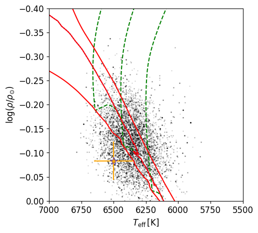
Figure 5: The best fitting evolutionary tracks and isochrones of WASP-180A obtained using bagemass. Black points: individual steps in the MCMC. Dotted blue line: Zero-Age Main Sequence (ZAMS) at best-fit [Fe/H]. Green dashed lines: evolutionary track for the best-fit [Fe/H] and mass, plus $1\sigma$ bounds. The lower-limit evolutionary track lies on top of the ZAMS, making it difficult to see. The Red lines: isochrone for the best-fit [Fe/H] and age, plus $1\sigma$ bounds. Orange star: measured values of $T_{\rm eff}$ and $\rho_{*}$ for WASP-180A obtained in the spectral and photometric analyses respectively.

We also extract stellar isochrones from Marigo et al. (2017) for stellar ages in the range 10⁸–5$\times\,10^{9}$ yr, using the metallicity from spectral analysis ([Fe/H] $\sim$ 0.09) to estimate appropriate mass fractions, obtaining Z = 0.024 and Y = 0.27. These are displayed on a colour–magnitude diagram in Fig. 6 along with the positions of WASP-180A and WASP-180B. The position of WASP-180A implies a system age of $\sim$ 1 Gyr while the position of WASP-180B implies an age close to $\sim$ 3 Gyr. The positions of WASP-180A and WASP-180B in Fig. 6 imply approximate stellar masses of $\sim$ 1.3 $M_{\star}$ and $\sim$ 1.0 $M_{\star}$ respectively, leading to a mass ratio of $M_{\star,B}$/$M_{\star,A}$ $\approx$ 0.77.

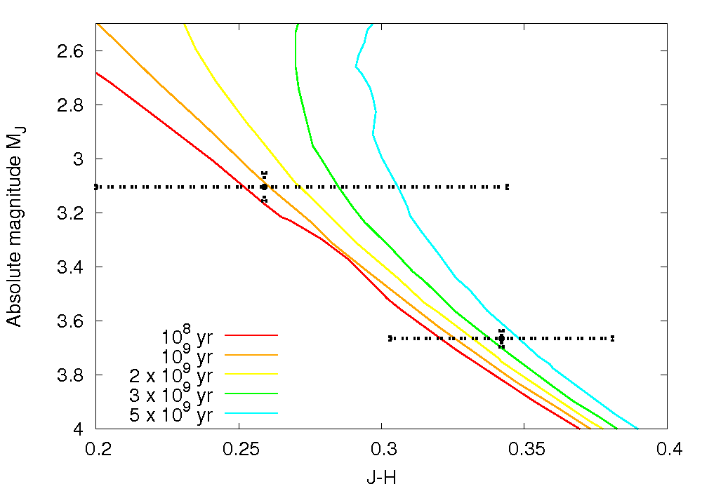
Figure 6: A colour-magnitude diagram showing the positions of WASP-180A and its comoving companion star with respect to isochrones from Marigo et al. (2017) for the ages 0.1, 1, 2, 3 and 5 Gyr (Z = 0.024 $\sim$ [Fe/H] = 0.09, Y=0.27).

Table 6: Results for the masses of WASP-180A and WASP-180B, and the age of the system.

Parameters from bagemass:
Parameter	Value
(Unit)
Age	1.22 $\pm$ 0.99
$M_{\star,A}$ ($M_{\rm\odot}$)	1.18 $\pm$ 0.08
$\rm[Fe/H]_{\rm init}$	–0.06 $\pm$ 0.16
Parameters from stellar isochrones:
$M_{\star,A}$ ($M_{\rm\odot}$)	1.3
$M_{\star,B}$ ($M_{\rm\odot}$)	1.0

7 Conclusions and discussion

WASP-180Ab is a 0.9 $\pm$ 0.1 $M_{\rm Jup}$, 1.24 $\pm$ 0.04 $M_{\rm Jup}$ hot Jupiter orbiting an F7 V star with $T_{\rm eff}$ = 6500 K and $v\sin i_{\star}$ = 19.9 km s^-1. The planet’s large radius is in line with the expectation for a Jovian-mass planet in a close orbit around a fairly hot star to be inflated due to the high level of irradiation (e.g. Enoch et al., 2012; Sestovic et al., 2018).

The orbit is misaligned and retrograde, with a projected obliquity of $\lambda$ = –157 $\pm$ 2 ^∘. This is also in line with known trends amongst hot Jupiters orbiting hot stars, since the majority of such planets are found to be in misaligned orbits (e.g. Winn et al., 2010; Albrecht et al., 2012; Dai & Winn, 2017; Triaud, 2017).

WASP-180 is a known binary system. We can ask whether the secondary, WASP-180B, is responsible for the retrograde, misaligned orbit seen in WASP-180Ab, through having induced Lidov-Kozai oscillations leading to high-eccentricity migration of the planet. While this effect has long been thought able to produce such orbits, the pathways leading from high-eccentricity migration to the observed distribution of system obliquities are still a topic of avid research (e.g. Anderson et al., 2016; Storch et al., 2017). Anderson et al. (2016) places an upper limit on the final period of a hot Jupiter which has migrated due to Lidov-Kozai oscillations of $P_{\rm orb}$ < 4 days, while Petrovich (2015) finds that the stellar separations of binaries with hot Jupiters are preferentially in the range 400–1500 AU, and so with $P_{\rm orb}$ = 3.4 days and an estimated stellar separation of 1200 AU it is feasible for WASP-180Ab to have formed in this way. Anderson et al. (2016) also finds that the expected timescale required for the migration of a hot Jupiter of 1 M_Jup via Lidov-Kozai oscillations is in the range $\sim$0.5–5 Gyr, with lower mass planets taking longer to migrate. The system age of 1.2 $\pm$ 1.0 Gyr is consistent with being within this range. It is possible that some eccentricity could remain, however, and our measured upper limit of $e$ < 0.27 at 95% confidence implies a possibly eccentric, but likely near circular orbit.

WASP-180Ab has $T_{\rm eff}$ = 6500 K and $v\sin i_{\star}$ = 19.9 $\pm$ 0.6 km s^-1. Another example of a hot Jupiter in a binary system with an early-type host star is KELT-19Ab, with $T_{\rm eff}$ = 7500 K and $v\sin i_{\star}$ = 84 $\pm$ 2 km s^-1 (Siverd et al., 2018). KELT-19Ab has a measured obliquity of $\lambda$ = –179^∘ and so is also on a retrograde orbit. KELT-19Ab is also similar to WASP-180Ab in that the primary and secondary stars in the system are of similar brightness. Such systems are rare, likely due to selection bias. Others include K2-29b (Santerne et al., 2016) and HAT-P-20b (Bakos et al., 2011).

Also, Ngo et al. (2015); Piskorz et al. (2015); Ngo et al. (2016) studied known exoplanet systems with FGK host stars, searching for previously unseen stellar companions and attempting to find a correlation between the presence of a distant stellar companion and the measured obliquity and eccentricity of a hot Jupiter’s orbit. They find no evidence of such a trend and conclude that, although a significant fraction of hot Jupiters reside in wide binary systems, fewer than 20% of hot Jupiters could have ended up in their current orbits as a result of Lidov-Kozai oscillations. Although both KELT-19Ab and WASP-180Ab are in misaligned, retrograde orbits, this is not necessarily related to the fact that they are in binary systems, since the tendency for hot Jupiters orbiting hot stars to be misaligned is well established (Winn et al., 2010; Albrecht et al., 2012).

The strength of the planet signal in tomography for WASP-180Ab makes it a potential candidate for looking for differential rotation following the RM reloaded technique of Cegla et al. (2016a), through which the effects of differential rotation and the perturbation due to the planet can be disentangled. To bring out the effect of differential rotation on the spectroscopic transit more clearly, the higher spectral resolution and greater light collecting power of ESPRESSO on the VLT would be of use.

References

- Albrecht et al. (2012) Albrecht S., et al., 2012, ApJ, 757, 18
- Anderson et al. (2016) Anderson K. R., Storch N. I., Lai D., 2016, MNRAS, 456, 3671
- Bakos et al. (2011) Bakos G. Á., et al., 2011, ApJ, 742, 116
- Barkaoui et al. (2017) Barkaoui K., Gillon M., Benkhaldoun Z., Emmanuel J., Elhalkouj T., Daassou A., Burdanov A., Delrez L., 2017, in Journal of Physics Conference Series. p. 012073, doi:10.1088/1742-6596/869/1/012073
- Barkaoui et al. (2019) Barkaoui K., et al., 2019, AJ, 157, 43
- Blackwell & Shallis (1977) Blackwell D. E., Shallis M. J., 1977, MNRAS, 180, 177
- Brown et al. (2017) Brown D. J. A., et al., 2017, MNRAS, 464, 810
- Bruntt et al. (2010) Bruntt H., et al., 2010, MNRAS, 405, 1907
- Burdanov et al. (2018) Burdanov A., Delrez L., Gillon M., Jehin E., 2018, SPECULOOS Exoplanet Search and Its Prototype on TRAPPIST. Springer International Publishing, Cham, pp 1–17, doi:10.1007/978-3-319-30648-3_130-1, https://doi.org/10.1007/978-3-319-30648-3_130-1
- Casagrande & VandenBerg (2014) Casagrande L., VandenBerg D. A., 2014, MNRAS, 444, 392
- Casagrande & VandenBerg (2018) Casagrande L., VandenBerg D. A., 2018, MNRAS, 475, 5023
- Cegla et al. (2016a) Cegla H. M., Lovis C., Bourrier V., Beeck B., Watson C. A., Pepe F., 2016a, A&A, 588, A127
- Cegla et al. (2016b) Cegla H. M., Oshagh M., Watson C. A., Figueira P., Santos N. C., Shelyag S., 2016b, ApJ, 819, 67
- Chambers et al. (2016) Chambers K. C., et al., 2016, arXiv e-prints,
- Claret (2000) Claret A., 2000, A&A, 363, 1081
- Claret (2004) Claret A., 2004, A&A, 428, 1001
- Collier Cameron et al. (2007) Collier Cameron A., et al., 2007, MNRAS, 380, 1230
- Collier Cameron et al. (2010) Collier Cameron A., Bruce V. A., Miller G. R. M., Triaud A. H. M. J., Queloz D., 2010, MNRAS, 403, 151
- Cutri et al. (2003) Cutri R. M., et al., 2003, VizieR Online Data Catalog, 2246
- Dai & Winn (2017) Dai F., Winn J. N., 2017, AJ, 153, 205
- Doyle et al. (2013) Doyle A. P., et al., 2013, MNRAS, 428, 3164
- Doyle et al. (2014) Doyle A. P., Davies G. R., Smalley B., Chaplin W. J., Elsworth Y., 2014, MNRAS, 444, 3592
- Enoch et al. (2012) Enoch B., Collier Cameron A., Horne K., 2012, A&A, 540, A99
- Epchtein et al. (1997) Epchtein N., et al., 1997, The Messenger, 87, 27
- Evans et al. (2018) Evans D. F., et al., 2018, A&A, 610, A20
- Gaia Collaboration et al. (2016) Gaia Collaboration et al., 2016, A&A, 595, A1
- Gaia Collaboration et al. (2018) Gaia Collaboration et al., 2018, A&A, 616, A1
- Gray & Corbally (2014) Gray R. O., Corbally C. J., 2014, AJ, 147, 80
- Green et al. (2014) Green G. M., et al., 2014, ApJ, 783, 114
- Green et al. (2015) Green G. M., et al., 2015, ApJ, 810, 25
- Gustafsson et al. (2008) Gustafsson B., Edvardsson B., Eriksson K., Jørgensen U. G., Nordlund Å., Plez B., 2008, A&A, 486, 951
- Hellier et al. (2011) Hellier C., et al., 2011, in European Physical Journal Web of Conferences. p. 01004 (arXiv:1012.2286), doi:10.1051/epjconf/20101101004
- Hirano et al. (2011) Hirano T., Suto Y., Winn J. N., Taruya A., Narita N., Albrecht S., Sato B., 2011, ApJ, 742, 69
- Jehin et al. (2011) Jehin E., et al., 2011, The Messenger, 145, 2
- Marigo et al. (2017) Marigo P., et al., 2017, ApJ, 835, 77
- Mason et al. (2001) Mason B. D., Wycoff G. L., Hartkopf W. I., Douglass G. G., Worley C. E., 2001, AJ, 122, 3466
- Maxted et al. (2011) Maxted P. F. L., et al., 2011, PASP, 123, 547
- Maxted et al. (2015) Maxted P. F. L., Serenelli A. M., Southworth J., 2015, A&A, 575, A36
- Ngo et al. (2015) Ngo H., et al., 2015, ApJ, 800, 138
- Ngo et al. (2016) Ngo H., et al., 2016, ApJ, 827, 8
- Niels Bohr Institute et al. (2014) Niels Bohr Institute Institute of Astronomy C., Real Instituto y Observatorio de La Armada 2014, VizieR Online Data Catalog, 1327
- Pepe et al. (2002) Pepe F., et al., 2002, The Messenger, 110, 9
- Petrovich (2015) Petrovich C., 2015, ApJ, 799, 27
- Piskorz et al. (2015) Piskorz D., Knutson H. A., Ngo H., Muirhead P. S., Batygin K., Crepp J. R., Hinkley S., Morton T. D., 2015, ApJ, 814, 148
- Pollacco et al. (2006) Pollacco D. L., et al., 2006, PASP, 118, 1407
- Pollacco et al. (2008) Pollacco D., et al., 2008, MNRAS, 385, 1576
- Pont et al. (2011) Pont F., Husnoo N., Mazeh T., Fabrycky D., 2011, MNRAS, 414, 1278
- Queloz et al. (2001) Queloz D., et al., 2001, The Messenger, 105, 1
- Santerne et al. (2016) Santerne A., et al., 2016, ApJ, 824, 55
- Sestovic et al. (2018) Sestovic M., Demory B.-O., Queloz D., 2018, A&A, 616, A76
- Siverd et al. (2018) Siverd R. J., et al., 2018, AJ, 155, 35
- Stassun & Torres (2018) Stassun K. G., Torres G., 2018, ApJ, 862, 61
- Storch et al. (2017) Storch N. I., Lai D., Anderson K. R., 2017, MNRAS, 465, 3927
- Temple et al. (2017) Temple L. Y., et al., 2017, MNRAS, 471, 2743
- Temple et al. (2018) Temple L. Y., et al., 2018, MNRAS, 480, 5307
- Temple et al. (2019) Temple L. Y., et al., 2019, AJ, 157, 141
- Triaud (2017) Triaud A. H. M. J., 2017, The Rossiter–McLaughlin Effect in Exoplanet Research. Springer International Publishing, Cham, pp 1–27, doi:10.1007/978-3-319-30648-3_2-1, https://doi.org/10.1007/978-3-319-30648-3_2-1
- Weiss & Schlattl (2008) Weiss A., Schlattl H., 2008, Ap&SS, 316, 99
- Winn et al. (2010) Winn J. N., Fabrycky D., Albrecht S., Johnson J. A., 2010, ApJ, 718, L145