Derivation of a Langevin equation in a system with multiple scales: the case of negative temperatures

Abstract

We consider the problem of building a continuous stochastic model, i.e. a Langevin or Fokker-Planck equation, through a well-controlled coarse-graining procedure. Such a method usually involves the elimination of the fast degrees of freedom of the “bath” to which the particle is coupled. Specifically, we look into the general case where the bath may be at negative temperatures, as found–for instance–in models and experiments with bounded effective kinetic energy. Here, we generalise previous studies by considering the case in which the coarse-graining leads to (i) a renormalisation of the potential felt by the particle, and (ii) spatially dependent viscosity and diffusivity. In addition, a particular relevant example is provided, where the bath is a spin system and a sort of phase transition takes place when going from positive to negative temperatures. A Chapman-Enskog-like expansion allows us to rigorously derive the Fokker-Planck equation from the microscopic dynamics. Our theoretical predictions show an excellent agreement with numerical simulations.

Introduction.- Systems with negative temperature typically appear in experiments or models where the effective kinetic and potential energies are limited and therefore the microcanonical entropy can be non-monotonic in the energy landau_statistical_2013; dunkel_consistent_2014; vilar_communication:_2014; frenkel_gibbs_2015; puglisi_temperature_2017. Examples are found in many physical contexts, including nuclear spins purcell_nuclear_1951; hakonen_negative_1994, fluid dynamics onsager_statistical_49 and trapped ultra-cold atoms rapp_equilibration_2010; braun_negative_2013. In these systems, the presence of negative temperatures is seen without ambiguities when observing certain degrees of freedom: for instance the single particle momentum distribution may take the typical form of an “inverted” Maxwell-Boltzmann distribution, of course with cut-off values at the boundaries cerino_consistent_2015.

It is worth recalling that negative values of temperature-like variables also arise in other physical frameworks, for example, within Edwards’s statistical mechanics description of dense granular media  edwards_theory_1989; mehta_statistical_1989; baule_edwards_2018. Therein, the role analogous to that of the temperature is played by the compactivity $X$, which is defined by $X^{-1}=\partial S(V)/\partial V$, where $S(V)$ is the total number of stable configurations for a given volume $V$. Since $S(V)$ is not a monotonic function of $V$, negative compactivities arise and correspond to packings that are looser than those characterised by positive values of $X$  brey_thermodynamic_2000; brey_closed_2003; ciamarra_random_2008; briscoe_jamming_2010.

Once the thermodynamics and the statistical mechanics of a class of systems has been understood, it is a natural question to wonder about their (statistical) dynamical description. A classical problem is that of deducing stochastic equations for the dynamics of slow degrees of freedom, for example a Langevin equation (LE) for the evolution of the position and/or momentum of a tagged massive particle zwanzig_nonlinear_1973. In the following, by LE we mean a stochastic differential equation, which corresponds to a continuous Markov process van_kampen_stochastic_1992. It is important to recall that analytical derivations thereof, through some kind of coarse-graining procedures, from the equations of the “microscopic” dynamics–e.g. Hamilton equations, Liouville equation, Boltzmann equation, etc.–are possible only in few special cases. A relevant alternative is to assume some form of LE with few parameters, based upon some previous theoretical knowledge of the investigated problem, and then estimate those parameters from numerical or experimental data through a proper inferring procedure. A discussion of such an approach and its many practical subtleties is given in Ref. baldovin_langevin_2018.

In the case of systems with negative temperature, a LE for a massive particle has already been considered by some of us in baldovin_langevin_2018. Therein, it was assumed that the parameters appearing in the LE–viscosity and noise amplitude–were constant. In general, however, it may happen that there is a coupling of the transport coefficients of the LE with the particle position, depending upon the particular form of the global Hamiltonian. Moreover, in such a previous investigation, a procedure to infer the viscosity–or noise amplitude–from the Hamiltonian of the total system was not provided: on the contrary, it was shown the fair success of an inference recipe of LE parameters from numerical data.

In the present paper, we consider a more general case that includes, in addition to possible negative temperatures, (i) a renormalisation of the potential felt by the heavy particle, and (ii) inhomogeneous LE parameters. The usual Einstein-like relation between viscosity and noise amplitude is confirmed by simply assuming equilibrium, with the particular form of kinetic energy not playing any crucial role. Afterwards, as an example, we investigate a Hamiltonian system comprising a slow continuous degree of freedom coupled to a bath of spins. A Chapman-Enskog-like coarse-graining procedure allows us to derive the LE for the slow degrees of freedom, which leads to both a renormalised potential and non-uniform viscosity and noise amplitudes, obeying the Einstein relation mentioned before. Interestingly, a phase transition–in a sense to be specified below–stems from the renormalisation of the potential, when the temperature crosses from positive to negetive values. Numerical simulations of the total Hamiltonian systems and the LE confirm our theoretical picture.

Renormalised potential and generalised Einstein-relation between viscosity and diffusivity.- Let us consider a system comprising a “heavy” particle with canonical variables $\Gamma\equiv(x,p)$ and a bath characterised by some variables that we denote by $\bm{z}$. The Hamiltonian of this system is assumed to have the form

$$H(\Gamma,\bm{z})=K(p)+U(x)+H_{N}(\bm{z})+V_{I}(x,\bm{z}),$$ (1)

where $K$ and $U$ are the “kinetic energy” of the slow particle and its external confining potential, respectively, $H_{N}$ is the Hamiltonian of the bath, and finally $V_{I}$ is the potential for the interaction between the heavy particle and the bath. The bath variables $\bm{z}$ can be, for example, positions and momenta of $N$ “light”’ particles or Ising variables of $N$ “fast” spins.

At equilibrium at temperature $T$, the probability distribution function (PDF) for the whole system is given by the canonical distribution, $\mathcal{P}_{\text{s}}(\Gamma,\bm{z})=Z^{-1}\exp[-\beta H(\Gamma,\bm{z})]$, where $Z$ is the partition function and $\beta$ is the inverse of the temperature–we are taking Boltzmann’s constant $k_{B}=1$. The marginal PDF for the particle variables is then given by

$$f_{\text{s}}(\Gamma)=Z^{-1}e^{-\beta[K(p)+U_{R}(x)]},\quad U_{R}(x)=U(x)+\mathcal{F}_{\text{b}}(x),$$ (2a)

$$e^{-\beta\mathcal{F}_{\text{b}}(x)}\equiv\int d\bm{z}\,e^{-\beta[H_{N}(\bm{z})+V_{I}(x,\bm{z})]}.$$ (2b)

Note that, in general, the integration over the bath variables renormalises the potential felt by the particle. The additional term $\mathcal{F}_{\text{b}}(x)$ is the free energy of the bath for given values of the particle variables.

Now we turn our attention to the dynamics. The evolution equations for $(x,p)$ read

$$\dot{x} =\partial_{p}H=K^{\prime}(p)$$ (3a)

$$\dot{p} =-\partial_{x}H=-U^{\prime}(x)-\partial_{x}V_{I}(x,\bm{z}),$$ (3b)

where the prime indicates the relevant derivative for functions that only depend on one variable. At this point, we introduce the hypothesis of time-scale separation: the heavy particle variables $(x,p)$ are assumed to evolve much slower than the bath variables $\bm{z}$. In this regime, the term $\partial_{x}V_{I}$ is expected to be described by a “viscous term”–only function of $(x,p)$–plus a “noisy term”. In other words, we seek to generalise the Klein-Kramers equation to systems with a generic form of $K(p)$, which may allow for the existence of negative temperatures.

Following the above discussion, our candidate equation has the generic form

$$\dot{x}=K^{\prime}(p),\qquad\dot{p}=-U^{\prime}(x)+B(\Gamma,t),$$ (4)

in which $B(\Gamma,t)$ is the effective force–which contains also a noisy term–on the particle stemming from the interaction with the bath. Going from Eq. (3b) to (4) implies conditional averages over the fast degrees of freedom, keeping fixed the slow variables. Therefore, the statistical properties of the coarse-grained force $B(\Gamma,t)$ depend in general on both $x$ and $p$.

The original Langevin-Klein-Kramers equation equation predicts a linear–or additive–form for $B$, namely $B(\Gamma,t)=-\gamma p+\sqrt{2D}\xi(t)$. Therein, $\xi(t)$ is a Gaussian white noise, with $\langle\xi(t)\rangle=0$ and $\langle\xi(t)\xi(t^{\prime})\rangle=2D\delta(t-t^{\prime})$, and the two main parameters are the constant viscosity $\gamma>0$ and diffusivity $D>0$. When $K(p)$ is not quadratic in $p$, the simplest modification is replacing the viscous term $-\gamma p$ with $-\gamma K^{\prime}(p)$. This was done in baldovin_langevin_2018, where the usual Einstein relation $\gamma=\beta D$ was shown to hold also for $\beta<0$.

The coarse-graining over the bath variables may lead to a more general situation, which we analyse here. First, an additional effective external potential term may appear in $B(\Gamma,t)$, which we identify with $-\mathcal{F}^{\prime}_{\text{b}}(x)$ to be consistent with the equilibrium situation: if the bath variables were infinitely fast, the bath would remain exactly at equilibrium at all times and the particle would follow a deterministic motion under the force $-U^{\prime}_{R}(x)=-U^{\prime}(x)-\mathcal{F}^{\prime}_{\text{b}}(x)$ . Second, the viscosity and the diffusivity may be spatially dependent, i.e $\gamma=\gamma(x)$ and $D=D(x)$. Incorporating these two ingredients into our description, we end up with the following ansatz for the coarse-grained force

$$B(\Gamma,t)=-\mathcal{F}_{\text{b}}^{\prime}(x)-\gamma(x)K^{\prime}(p)+\sqrt{2D(x)}\xi(t).$$ (5)

The Fokker-Planck equation for the PDF $f(\Gamma,t)$ for the heavy particle is then

$$\partial_{t}f= -K^{\prime}(p)\partial_{x}f+U_{R}^{\prime}(x)\partial_{p}f$$

$$+\partial_{p}\left[\gamma(x)K^{\prime}(p)f+D(x)\partial_{p}f\right],$$ (6)

Following risken_solutions_1972, we can write the Fokker-Planck equation as a conservation law, $\partial_{t}f=-\nabla\cdot\bm{J}$, where $\bm{J}\equiv\{J_{x},J_{p}\}$ is the probability density current and $\nabla\cdot\bm{J}\equiv\partial_{x}J_{x}+\partial_{p}J_{p}$. Moreover, $\bm{J}$ can be split into its reversible and irreversible parts $\bm{J}_{\text{rev}}$ and $\bm{J}_{\text{irr}}$, specifically $\bm{J}_{\text{rev}}(\Gamma,t)=\{K^{\prime}(p)f(\Gamma,t),-U_{R}^{\prime}(x)f(\Gamma,t)\}$ and $\bm{J}_{\text{irr}}(\Gamma,t)=\{0,-\gamma(x)K^{\prime}(p)f(\Gamma,t)-D(x)\partial_{p}f(\Gamma,t)\}$.

The steady solution of the Fokker-Planck equation must be the equilibrium distribution $f_{\text{s}}(\Gamma)$ in Eq. (2a). On the one hand, substitution of the steady distribution into the Fokker-Planck equation always leads to $\nabla\cdot\bm{J}_{\text{rev},\text{s}}(\Gamma)\equiv 0$, with no particular requirements for the reversible part of the current. On the other hand, the condition $\nabla\cdot\bm{J}_{\text{irr},\text{s}}=0$ can be fulfilled only if $\bm{J}_{\text{irr},\text{s}}\equiv 0$, i.e., if detailed balance (DB) holds risken_solutions_1972. The DB condition leads to

$$\gamma(x)=\beta D(x),$$ (7)

which is a generalised Einstein relation for inhomogeneous viscosity and diffusivity.

An example with analytical derivation of the LE - As an example of the general case discussed before, we consider the following Hamiltonian for a slow particle coupled to a spin bath,

$$H(\Gamma,\bm{\sigma}) =K(p)+V(x,\bm{\sigma}),$$ (8a)

$$V(x,\bm{\sigma}) =U(x)-\mu\lambda(x)\sum_{j=1}^{N}\sigma_{j}.$$ (8b)

Above, $\bm{\sigma}\equiv(\sigma_{1},\sigma_{2},...,\sigma_{N})$ are spin variables, $\sigma_{j}=\pm 1$, $\mu$ is a constant, and $\lambda(x)$ is a certain function of $x$. Then, the spins $\bm{\sigma}$ are the bath variables $\bm{z}$ in Eq. (1), and the bath contribution to the Hamiltonian $H_{N}({\bm{z}})+V_{I}({x,\bm{z}})$ reduces to the term $-\mu\lambda(x)\sum_{j}\sigma_{j}$, i.e. the spins feel an inhomogeneous external field $\mu\lambda(x)$.

To start with, we discuss the equilibrium situation. Therein, the system as a whole is described by the canonical distribution $\mathcal{P}_{\text{s}}(\Gamma,\bm{\sigma})=Z^{-1}\exp\left[-\beta H(\Gamma,\bm{\sigma})\right]$. In this simple case, the specific form of the free energy of the bath $\mathcal{F}_{\text{b}}(x)$ for given values of the particle variables is

$$e^{-\beta\mathcal{F}_{\text{b}}(x)}=\left\{2\cosh\left[\beta\mu\lambda(x)\right]\right\}^{N}.$$ (9)

Moreover, we can also write the conditional probability of finding the spins in a configuration $\bm{\sigma}$ for given values of the particle variables as

$$\mathcal{P}^{\text{s}}(\bm{\sigma}|x)=e^{\beta\left[\mu\lambda(x)\sum_{j}\sigma_{j}+\mathcal{F}_{\text{b}}(x)\right]}.$$ (10)

Our notation makes it explicit that this conditional probability depends only on $x$. Also, we have that

$$\mathcal{F}^{\prime}_{\text{b}}(x)=-N\mu\lambda^{\prime}(x)\langle\sigma\rangle_{\text{s}}(x),\quad\langle\sigma\rangle_{\text{s}}(x)=\tanh\left[\beta\mu\lambda(x)\right]\,,$$ (11)

where $\langle\sigma\rangle_{\text{s}}(x)\equiv\sum_{\bm{\sigma}}\sigma_{j}\mathcal{P}^{\text{s}}(\bm{\sigma}|x)$, for any $j$.

Now, let us consider the dynamics. On the one hand, accordingly with our previous general discussion, the evolution equations for $(x,p)$ are

$$\dot{x}=\frac{\partial H}{\partial p}=K^{\prime}(p),\quad\dot{p}=-\frac{\partial H}{\partial x}=-\partial_{x}V(x,\bm{\sigma}),$$ (12)

where $\partial_{x}V(x,\bm{\sigma})=U^{\prime}(x)-\mu\lambda^{\prime}(x)\sum_{j}\sigma_{j}$. On the other hand, and for the sake os simplicity, we assume Glauber’s stochastic dynamics for the spins. We denote by $\mathcal{R}_{j}$ the operator that flips the $j$-th spin, leaving the remainder unchanged. The transition rate for the flipping of the $j$-th spin, i.e. from configuration $\bm{\sigma}$ to $\mathcal{R}_{j}\sigma$, is

$$W_{j}(\bm{\sigma}|x)=\frac{\alpha}{2}\left\{1-\sigma_{j}\tanh[\beta\mu\lambda(x)]\right\},$$ (13)

in which $\alpha$ is a characteristic rate glauber_time-dependent_1963. We can write a Liouville-master equation for the time evolution of the joint PDF $\mathcal{P}(\Gamma,\bm{\sigma},t)$,

$$\mathbb{W}(\bm{\sigma}|x)\mathcal{P}(\Gamma,\bm{\sigma},t)=\varepsilon\left[\partial_{t}+\mathcal{L}(\Gamma,\bm{\sigma})\right]\mathcal{P}(\Gamma,\bm{\sigma},t)\,.$$ (14)

We have introduced the linear operators

$$\mathbb{W}(\bm{\sigma}|x) \equiv\sum_{j=1}^{N}(\mathcal{R}_{j}-1)W_{j}(\bm{\sigma}|x),$$ (15a)

$$\mathcal{L}(\Gamma,\bm{\sigma}) \equiv K^{\prime}(p)\partial_{x}-\partial_{x}V(x,\bm{\sigma})\partial_{p}.$$ (15b)

Note the auxiliary $\varepsilon$ in front of the right-hand side (rhs) of Eq. (14), actually $\varepsilon=1$. Clearly, the canonical distribution is a time-independent solution of Eq. (14) .

Our idea is to derive an equation for the marginal PDF for the particle variables $f(\Gamma,t)=\sum_{\bm{\sigma}}\mathcal{P}(\Gamma,\bm{\sigma},t)$ when the spins are much faster than the “heavy” particle. Specifically, this means that $\omega_{0}/\alpha\ll 1$, with $\omega_{0}^{-1}$ being the characteristic time over which the “heavy” particle evolves. Instead of making this idea explicit by introducing dimensionless variables, we have employed an equivalent approach–usual in kinetic theory–by introducing the auxiliary $\varepsilon$ in front of the rhs of Eq. (14) .

Chapman-Enskog expansion.- We proceed with an expansion in powers of $\varepsilon$,

$$\mathcal{P}(\Gamma,\bm{\sigma},t)=\mathcal{P}^{\text{s}}(\bm{\sigma}|x)f(\Gamma,t)+\sum_{l=1}^{\infty}\varepsilon^{l}\,\mathcal{P}^{(l)}(\Gamma,\bm{\sigma},t).$$ (16)

We ensure $f(\Gamma,t)$ to be the exact marginal distribution of the particle by assuming $\sum_{\bm{\sigma}}\mathcal{P}^{(l)}(\Gamma,\bm{\sigma},t)=0$, $\forall l\geq 1$. It is the dynamical equation of $f(x,p,t)$–and not $f$ itself–that is expanded in powers of $\varepsilon$ in the Chapman-Enskog method resibois_classical_1977; bonilla_chapman-enskog_2000; bonilla_nonlinear_2009; neu_singular_2015; bonilla_unpublished_2019

$$\partial_{t}f(\Gamma,t)=\sum_{l=0}^{\infty}\varepsilon^{l}F^{(l)}(\Gamma,t)\,.$$ (17)

Truncating the above series at the lowest order ($l=0$), one has the “deterministic” (zero noise) approximation. The effect of the noise can be introduced in the simplest way by retaining the first two terms ($l=0,1$). This is what we do in the following .

Now, we list the equations obtained by inserting Eqs. (10), (16), and (17) into Eq. (14). Up to order $\varepsilon^{2}$,

$$\mathbb{W}(\bm{\sigma}|x)\mathcal{P}^{\text{s}}(\bm{\sigma}|x)f(\Gamma,t)=0,$$ (18a)

$$\mathbb{W}(\bm{\sigma}|x)\mathcal{P}^{(1)}(\Gamma,\bm{\sigma},t)=\mathcal{P}^{\text{s}}(\bm{\sigma}|x)F^{(0)}(\Gamma,t)$$

$$\qquad\qquad\qquad\qquad\qquad+\mathcal{L}(\Gamma,\bm{\sigma})\mathcal{P}^{\text{s}}(\bm{\sigma}|x)f(\Gamma,t),$$ (18b)

$$\mathbb{W}(\bm{\sigma}|x)\mathcal{P}^{(2)}(\Gamma,\bm{\sigma},t)=\mathcal{P}^{\text{s}}(\bm{\sigma}|x)F^{(1)}(\Gamma,t)$$

$$\quad\qquad\qquad\qquad\qquad\quad+\left[\partial_{t}+\mathcal{L}(\Gamma,\bm{\sigma})\right]\mathcal{P}^{(1)}(\Gamma,\bm{\sigma},t)\,.$$ (18c)

Equation (18a) (order of unity, $\varepsilon^{0}$) is an identity, because in Eq. (16) we have anticipated the zero-th order contribution to the expansion of $\mathcal{P}$ in powers of $\varepsilon$.

First, we resort to Eq. (18b) (order of $\varepsilon$) to obtain $F^{(0)}$ and $\mathcal{P}^{(1)}$. We bring to bear that the rhs of Eq. (18b) must be orthogonal to $\mathcal{P}^{\text{s}}(\bm{\sigma}|x)$, i.e. its sum over all the spin configurations vanishes, which entails that $F^{(0)}=-K^{\prime}(p)\partial_{x}f+\left[U^{\prime}(x)+\mathcal{F}^{\prime}_{\text{b}}(x)\right]\partial_{p}f$. Following our general discussion, there appears an extra force $-\mathcal{F}^{\prime}_{\text{b}}(x)$, given in this specific system by Eq. (11). In order to have a consistent limit as $N\to\infty$, the coupling constant $\mu$ between the particle and the spins must scale as $N^{-1/2}$ . With this scaling, we have that

$$F^{(0)}(\Gamma,t) =-K^{\prime}(p)\partial_{x}f(\Gamma,t)+U^{\prime}_{R}(x)\partial_{p}f(\Gamma,t)$$ (19a)

$$U_{R}(x) =U(x)-\frac{\beta}{2}\tilde{\mu}^{2}\lambda^{2}(x)\,,\quad\mu=\tilde{\mu}N^{-1/2},$$ (19b)

It is worth emphasising the emergence of the “renormalised” potential $U_{R}(x)$, once more accordingly with the general framework developed before.

Next, we substitute the obtained expressions for $F^{(0)}$ into Eq. (18b), and take into account that $\partial_{x}\mathcal{P}^{\text{s}}(\bm{\sigma}|x)=\beta\mu\lambda^{\prime}(x)\sum_{j}\left[\sigma_{j}-\langle\sigma\rangle_{\text{s}}(x)\right]\mathcal{P}^{\text{s}}(\bm{\sigma}|x)$ to write the following equation for $\mathcal{P}^{(1)}$,

$$\!\!\!\!\mathbb{W}(\bm{\sigma}|x)\mathcal{P}^{(1)}(\Gamma,\bm{\sigma},t) =\mu\lambda^{\prime}(x)\left[\beta K^{\prime}(p)f(\Gamma,t)+\partial_{p}f(\Gamma,t)\right]$$

$$\quad\times\sum_{j=1}^{N}\left[\sigma_{j}-\langle\sigma\rangle_{\text{s}}(x)\right]\mathcal{P}^{\text{s}}(\bm{\sigma}|x)\,.$$ (20)

Interestingly, this equation can be explicitly solved for $\mathcal{P}^{(1)}$, because it is easy to show that $\sum_{j}\left[\sigma_{j}-\langle\sigma\rangle_{\text{s}}(x)\right]\mathcal{P}^{\text{s}}(\bm{\sigma}|x)$ is an eigenvector of the operator $\mathbb{W}(\bm{\sigma}|x)$ corresponding to the eigenvalue $-\alpha$. Therefore,

$$\mathcal{P}^{(1)}(\Gamma,\bm{\sigma},t) =-\alpha^{-1}\mu\lambda^{\prime}(x)\left[\beta K^{\prime}(p)f(\Gamma,t)+\partial_{p}f(\Gamma,t)\right]$$

$$\quad\times\sum_{j=1}^{N}\left[\sigma_{j}-\langle\sigma\rangle_{\text{s}}(x)\right]\mathcal{P}^{\text{s}}(\bm{\sigma}|x).$$ (21)

Now, we make use of Eq. (18) to calculate $F^{(1)}$ : its rhs must also be orthogonal to $\mathcal{P}^{\text{s}}(\bm{\sigma}|x)$, i.e. the sum over all the spin configurations must vanish. Therefore, $F^{(1)}=-\mu\lambda^{\prime}(x)\sum_{\bm{\sigma}}\sum_{j}\sigma_{j}\partial_{p}\mathcal{P}^{(1)}$, from which (i) taking into account the explicit expression for $\mathcal{P}^{(1)}$ and (ii) considering the limit as $N\to\infty$, $F^{(1)}$ is reduced to

$$F^{(1)}(\Gamma,t)=\alpha^{-1}\left[\tilde{\mu}\lambda^{\prime}(x)\right]^{2}\partial_{p}\left[\beta K^{\prime}(p)f(\Gamma,t)+\partial_{p}f(\Gamma,t)\right]\,.$$ (22)

Fokker-Planck equation for $f(\Gamma,t)$.- Up to order $\varepsilon$, the evolution of the marginal distribution $f(\Gamma,t)$, is given by $\partial_{t}f=F^{(0)}+\varepsilon F^{(1)}$. We write the result in the limit as $N\to\infty$, with the scaling in Eq. (19b) and, moreover, we make $\varepsilon=1$ as we discussed before carrying out the Chapman-Enskog expansion. Making use of Eqs. (19) and (22), we arrive at

$$\partial_{t}f =-K^{\prime}(p)\partial_{x}f+U^{\prime}_{R}(x)\partial_{p}f$$

$$\quad+\alpha^{-1}\left[\tilde{\mu}\lambda^{\prime}(x)\right]^{2}\partial_{p}\left[\beta K^{\prime}(p)f+\partial_{p}f\right]\,$$ (23)

which is in complete agreement with the general picture we have developed before. In particular, comparison with Eq. (6) leads to identifying the viscosity and the diffusivity in terms of the microscopic parameters of the model,

$$D(x)=\alpha^{-1}\left[\tilde{\mu}\lambda^{\prime}(x)\right]^{2},\quad\gamma(x)=\beta D(x).$$ (24)

Of course, the stationary solution of Eq. (Derivation of a Langevin equation in a system with multiple scales: the case of negative temperatures) is the exact marginal equilibrium distribution $f_{\text{s}}(\Gamma)\propto e^{-\beta\left[K(p)+U_{R}(x)\right]}$, in accordance with Eq. (2a).

The Fokker-Planck equation (Derivation of a Langevin equation in a system with multiple scales: the case of negative temperatures) can be rewritten as a LE,

$$\dot{x}=K^{\prime}(p),\quad\dot{p}=-U^{\prime}_{R}(x)-\alpha^{-1}\left[\tilde{\mu}\lambda^{\prime}(x)\right]^{2}\beta K^{\prime}(p)+\xi(t),$$ (25)

in which $\xi(t)$ is a Gaussian white noise verifying

$$\langle\xi(t)\rangle=0\,,\quad\langle\xi(t)\xi(t^{\prime})\rangle=2\alpha^{-1}\left[\tilde{\mu}^{2}\lambda^{\prime}(x)\right]^{2}\delta(t-t^{\prime})\,.$$ (26)

In Eq. (25), the noise acts on the variable $p$ while $D(x)$ depends only on $x$, thus it is not multiplicative.

Numerical simulations.- In order to check the consistency of our theoretical scheme, we perform numerical simulations of the “exact” microscopic dynamics (14) in the $\alpha\gg 1$–fast spins–limit: our aim is to compare the measured values of significative observables to those predicted by the mesoscopic description provided by the Fokker-Planck equation (Derivation of a Langevin equation in a system with multiple scales: the case of negative temperatures). Specifically, we consider the following case

$$K(p)=1-\cos p,\quad U(x)=\left(1-\cos x\right)^{2},\quad\lambda(x)=\sin x\,.$$ (27)

The kinetic energy is inspired by the experiment in Ref. braun_negative_2013, where cold atoms in an optical lattice display both positive and negative temperatures. It has also been studied theoretically, for instance see cerino_consistent_2015; baldovin_langevin_2018.

For the microscopic dynamics, the spins are started from a completely random configuration. Then, for each time-step $dt$ thereof, our algorithm performs two actions: first, it evolves the state $(x,p)$ of the particle through a deterministic Velocity Verlet integration step; then it chooses one spin with uniform probability, and tries to flip it according to the Glauber dynamics (13). The probability of flipping the chosen spin $\sigma_{j}$ is given by $Ndt\,W_{j}(\bm{\sigma}|x)$; in order to keep it of the order of unity, we choose $dt=(\alpha N)^{-1}$ for our simulations.

As a first check of the validity of our description, we verify the renormalisation of the potential that arises in our theoretical framework. Specifically, we check the shape of the equilibrium PDF for the particle variables $(x,y)$, which is given by Eq. (2a). Making use of Eq. (19b) and (27), the renormalised potential $U_{R}(x)$ is

$$U_{R}(x)=(1-\cos x)^{2}-\frac{\beta}{2}\tilde{\mu}^{2}\sin^{2}x\,.$$ (28)

For positive temperatures, $U_{R}(x)$ corresponds to a bistable potential with symmetric minima at $x\in[-\pi,\pi]$ verifying $\cos x=2/(2+\beta\tilde{\mu}^{2})$ and maxima at $x=0,\pm\pi$, whereas for negative temperatures $U_{R}(x)$ has only one minimum at $x=0$ and attains its maximum value at $x=\pm\pi$. Thus, the most probable value of $x$–given by the maximum of $\exp[-\beta U_{R}(x)]$–changes discontinuously from $x=\pm\tilde{\mu}\sqrt{\beta}$ for $\beta=0^{+}$ to $x=\pm\pi$ for $\beta=0^{-}$.

In Fig. 1, we show the histograms of $x$ and $p$ at equilibrium, for two values of the temperature with opposite signs: the agreement between the numerical and the theoretical results are excellent. By fitting each plot with the corresponding Boltzmann factor, we infer values of the parameter $\beta$ that are compatible with the original ones used in the simulations, within the confidence interval for the fit. Note that the most probable value of momentum is $\pm\pi\neq 0$ for $\beta<0$, but this is compatible with stationarity: there is no average drift since $\dot{x}=\partial H/\partial p=\sin p$.

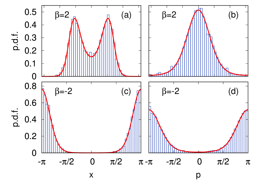
Figure 1: Equilibrium PDF of the particle variables $(x,p)$. The top (bottom) panels correspond to $\beta=2$ ($\beta=-2$). Histograms are computed from numerical simulations of the microscopic dynamics (14); red solid lines are the best fits to the Boltzmann distribution (2a). Parameters: $N=10^{4}$, $\alpha=10$, $\mu=10^{-2}$, $dt=(\alpha N)^{-1}$.

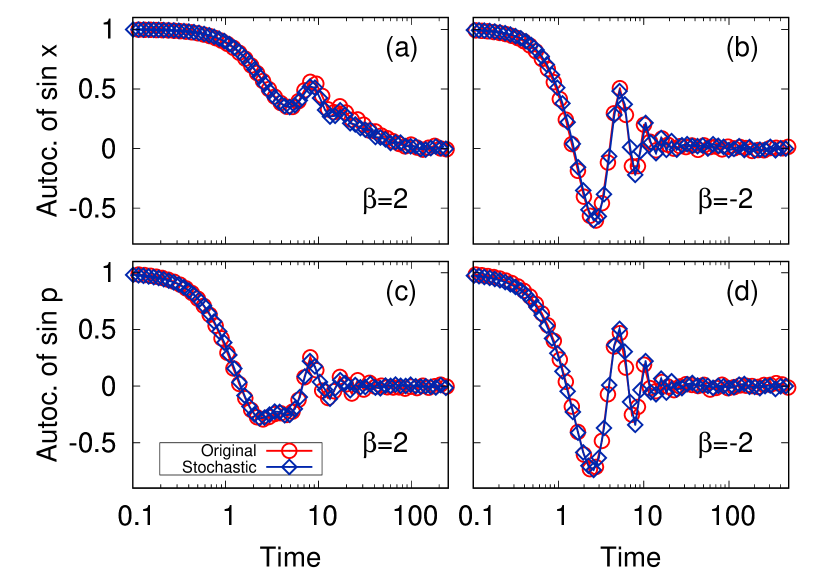
Figure 2: Equilibrium autocorrelation functions. Specifically, we consider two observables, $\sin x$ above and $\sin p$ below, for $\beta=2$ (left panels) and $\beta=-2$ (right panels). Red circles represent the simulations of the original dynamics (14), whereas blue diamonds are the numerical integration of the Fokker-Plank equation (Derivation of a Langevin equation in a system with multiple scales: the case of negative temperatures), with a time-step $h=10^{-4}$. Other parameters as in Fig. 1.

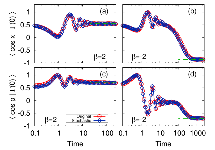
Figure 3: Relaxation to equilibrium. We plot the time evolution of the averages of $\cos x$ (top) and $\cos p$ (bottom), for $\beta=2$ (left panels) and $\beta=-2$ (right panels). In all cases, the particle starts from the initial condition $\Gamma(0)=(x(0),p(0))=(1,1)$. As in Fig. 2, the original dynamics (red circles) is compared with the Fokker-Planck equation (blue diamonds), with a time-step $h=10^{-4}$. Other parameters as in Fig. 1. Green dashed lines are $\langle\cos x\rangle$ and $\langle\cos p\rangle$ analytically computed averaging over the theoretical equilibrium distributions.

Second, we check the accuracy of the derived Fokker-Planck equation for describing the dynamics of the particle variables. More concretely, it is how the dynamical quantities obtained from Fokker-Planck compare with those obtained from the exact dynamics that we are interested in. With this aim, we numerically integrate Eq. (25) using a standard algorithm for stochastic differential equations mannella_fast_1989–in its variant of order $h^{3/2}$, where $h$ is the time-step.

Several time-dependent quantities computed from the Fokker-Planck equation (Derivation of a Langevin equation in a system with multiple scales: the case of negative temperatures) are compared with those obtained by simulating the original Liouville-master equation (14). In Fig. 2, we look into time correlation functions at equilibrium, namely, into the autocorrelations of $\sin x$ and $\sin p$. The qualitative difference between panels (a) and (b) can be related to the shape of the free energy, which is different for positive and negative temperatures. When it is bi-stable ($\beta>0$), the time needed to cross zero is longer and thus oscillations are hindered. In Fig. 3, we study the relaxation to equilibrium of some dynamical observables. In particular, we have evaluated $\langle\cos x\rangle$ and $\langle\cos p\rangle$, conditioned to fixed initial values of the particle variables $\Gamma(0)\equiv(x(0),p(0))$. In both cases, the agreement is evident.

Concluding remarks.- In conclusion, we have generalised the problem of deriving a LE to non-standard forms of the Hamiltonian that also allow for absolute negative temperatures. The LE obtained here satisfies a generalised Einstein relation that has been shown to apply for (i) arbitrary spatial dependence of the transport coefficients, and (ii) situations in which the potential felt by the particle is renormalised as a consequence of its interaction with the bath. Such a renormalisation is relevant when the eliminated fast degrees of freedom change the potential felt by the particle .

A particular example is treated in detail through a Chapman-Enskog-like coarse-graining procedure, which provides exact expressions for the transport coefficients. This specific case is in complete agreement with the general picture and, in addition, presents a transition from one-basin to bi-stable free energy when going from positive to negative temperatures.