Bose-Einstein condensation in spherically symmetric traps

Abstract

We present a pedagogical introduction to Bose-Einstein condensation in traps with spherical symmetry, namely the spherical box and the thick shell, sometimes called bubble trap. In order to obtain the critical temperature for Bose-Einstein condensation, we describe how to calculate the cumulative state number and density of states in these geometries, using numerical and analytical (semi-classical) approaches. The differences in the results of both methods are a manifestation of Weyl’s theorem, i.e., they reveal how the geometry of the trap (boundary condition) affects the number of the eigenstates counted. Using the same calculation procedure, we analyzed the impact of going from three-dimensions to two-dimensions, as we move from a thick shell to a two-dimensional shell. The temperature range we obtained, for most commonly used atomic species and reasonable confinement volumes, is compatible with current cold atom experiments, which demonstrates that these trapping potentials may be employed in experiments.

Keywords: Bose-Einstein condensation, cold atoms, critical temperature, trapping potential, bubble trap.

I Introduction

A Bose-Einstein condensate (BEC) corresponds to the macroscopic occupation of the lowest energy quantum state by the particles of a system Bose (1924). Bose-Einstein condensation occurs when the system is cooled below a critical temperature $T_{c}$ and the mean interparticle distance $\bar{l}=\rho^{-1/3}$, $\rho$ being the number density of $N$ particles in a volume $V$, becomes comparable to the de Broglie wavelength,

$$\lambda=\frac{h}{Mv},$$ (1)

where $M$ is the mass of the atoms, and $v=\sqrt{k_{B}T/M}$ is their thermal velocity, $k_{B}$ being the Boltzmann constant. Imposing $\lambda\sim\bar{l}$ implies that a homogeneous gas will undergo a Bose-Einstein condensation at a temperature

$$T_{c}\sim\frac{h^{2}\rho^{2/3}}{Mk_{B}}.$$ (2)

This simple qualitative argument differs from the accurate result only by a factor of $\approx$ 3.3 Pethick and Smith (2002).

The first experimental realizations of Bose-Einstein condensation in dilute gases were achieved in 1995 Anderson et al. (1995); Bradley et al. (1995); Davis et al. (1995), and currently several laboratories around the world produce BECs on a daily basis. One feature of experiments with cold atomic gases that led to rapid advances in the field is the ability to control the parameters of the system Griffin et al. (1996); Ketterle et al. (1999). The interatomic interactions and trapping potentials can be changed by external electromagnetic fields, with unprecedented control. Although harmonic potentials are the most commonly used traps in experiments, other geometries, such as box traps Gaunt et al. (2013), recently became available.

In this work we are interested in dilute gases. Here we study a BEC trapped in spherically symmetric potentials, the spherical box and the thick shell, sometimes called bubble trap. Our theoretical studies are motivated by the experimental possibility of confining the atoms in this kind of trap Zobay and Garraway (2001, 2004); Garraway and Perrin (2016), which has to be inserted in a microgravity setting to produce a spherical atom distribution Elliott et al. (2018). We determined the cumulative state number and density of states in these geometries in order to calculate the critical temperature for Bose-Einstein condensation. The temperature range we obtained is compatible with current cold atom experiments, which demonstrates that these trapping potentials may be employed in experiments.

We also discuss, very briefly, the effects of reducing the dimensionality of the system of interest from 3D to 2D, which is what happens when the thickness of the shell goes to zero. The study of cold gases has proven to be a very rich research field, and the investigation of low-dimensional systems has become an active area in this context Giorgini et al. (2008); Bloch et al. (2008).

We wrote this manuscript in a pedagogical way, hoping that dedicated undergraduate students will find all the necessary ingredients to reproduce the results presented here. Moreover, we wish to show that even if some problems in statistical physics do not have analytical solutions, numerical methods offer some insight into the underlying physics of the system, as we will show here.

This work is structured as it follows. In Sec. II we introduce the concepts related to the cumulative state number and density of states. We begin by calculating the energy levels of a particle in a rigid box, Sec. II.1; then we show how the density of states can be obtained from the cumulative state number, Sec. II.2; we write expressions for these quantities in the high-energy limit, Sec. II.3, and semi-classical approximations, Sec. II.4. Weyl’s theorem is presented in Sec. II.5. Bose-Einstein condensation is introduced in Sec. III, where we derive the expression for the critical temperature in three-dimensions. Sec. IV deals with the solution of Schrödinger’s equation for a spherically symmetric potential, which is then applied to two different trapping potentials: the spherical box and the thick shell, Secs. V and VI, respectively. The critical temperatures are calculated in Sec. VII, for three-dimensional, Sec. VII.1, and two-dimensional systems, Sec. VII.2. Finally, we summarize our findings in Sec. VIII. Appendix A deals with the generalization of the critical temperature expression for $D$ dimensions.

II Cumulative state number and density of states

II.1 Particle in a rigid box

The concept of density of states (DOS) is ubiquitous to many areas of physics, such as: specific heat calculations, black-body radiation, phonon spectra, reaction rates in nuclear physics, and many more. For a pedagogical overview the reader is referred to Ref. Mulhall and Moelter (2014). In this work, we are going to use the DOS to calculate the critical temperature of a trapped BEC.

In statistical physics many quantities can be expressed as integrations over the phase space, which can be very complicated. An alternative is to replace the variables in terms of the energy of the system, thus replacing the volume in phase space by a weight factor in the energy integral. This weight factor is the density of states, which typically makes the integrals more tractable.

Let us begin with the case of a particle in a rigid box, that is, subjected to a potential which is zero inside the box and infinite outside it. Although it is a very simple example, it exhibits the nonclassical behavior expected from a quantum mechanical problem, and it also serves as a building block to more complex examples (scattering, double-well, among many others). A nonrelativistic particle of mass $M$ inside a one-dimensional box of size $L$ has energy levels given by Griffiths and Schroeter (2018)

$$\varepsilon_{n}^{\rm 1D}=\frac{\hbar^{2}}{2M}\frac{\pi^{2}}{L^{2}}n_{x}^{2}=\varepsilon_{0}n_{x}^{2},$$ (3)

where we defined $\varepsilon_{0}=\pi^{2}\hbar^{2}/(2mL^{2})$ and $n_{x}$ is an integer. In a two-dimensional square box of sides $L$, the energy levels are simply $\varepsilon_{n}^{\rm 2D}=\varepsilon_{0}(n_{x}^{2}+n_{y}^{2})$, where we introduced an extra integer $n_{y}$ to take into account the $y$-dimension. Finally, a straightforward generalization to three-dimensions yields $\varepsilon_{n}^{\rm 3D}=\varepsilon_{0}(n_{x}^{2}+n_{y}^{2}+n_{z}^{2})$.

II.2 $n$-space representation

For the following discussion we are going to assume the two-dimensional case because its visualization is easier, but the arguments hold in the other cases. The momentum space is defined by the variables $p_{x}$ and $p_{y}$, but they only differ from $n_{x}$ and $n_{y}$ by a constant, $p_{i}=\hbar k_{i}=n_{i}\pi\hbar/L$ with $i=x$, $y$. So let us call this space, defined by $n_{x}$ and $n_{y}$, $n$-space. We can think of each quantum number being a line, and the intersection of the lines correspond to the allowed quantum states $(n_{x},n_{y})$. In Fig. 1 we represent the two-dimensional $n$-space, and for each quantum state we write the energy $\varepsilon_{n}^{\rm 2D}$ in units of $\varepsilon_{0}$. A curve with constant energy or, conversely, constant $n^{2}$, is given by $n=\sqrt{n_{x}^{2}+n_{y}^{2}}$. When independent states correspond to the same energy we say they are degenerate. This is illustrated in Fig. 1 by the quarter circle $n=\sqrt{n_{x}^{2}+n_{y}^{2}}=5$ which intersects two grid points, (3,4) and (4,3), corresponding to the two degenerate energy states. Notice, however, that not all energies are allowed, for example $n=\sqrt{n_{x}^{2}+n_{y}^{2}}=6$ does not intersect any points.

Figure 1: Energies, in units of $\varepsilon_{0}^{\rm 2D}$, of a particle in a 2D square box as a function of the integers $n_{x}$ and $n_{y}$. The quarter circles correspond to $n=\sqrt{n_{x}^{2}+n_{y}^{2}}=$ 5 and 6. Notice that $n=5$ intersects two grid points, (3,4) and (4,3), corresponding to the degeneracy of this energy level, whereas $n=6$ does not intersect any points.

If we list all the allowed energies $\varepsilon$ of our system, or more practically all the possible energies up to a cutoff, and their corresponding degeneracies $d(\varepsilon)$, we could make a plot of $d(\varepsilon)$, which would correspond to the “number of states with energy $\varepsilon$” vs $\varepsilon$. This graph would be a series of spikes, at the allowed energies $\varepsilon$, each with height $d(\varepsilon)$. At this point it is helpful to introduce a new quantity, the cumulative state number $\mathcal{N}(\varepsilon)$ defined as the number of states with energy less than or equal to $\varepsilon$. Its graph is a staircase where each step has a height $d(\varepsilon)$ and a width given by the gap between two consecutive energy levels.

Finally, we can introduce the density of states function $g(\varepsilon)$ as being related to the cumulative state number through $g(\varepsilon)d\varepsilon=d\mathcal{N}(\varepsilon)$, so we identify $g(\varepsilon)$ with the slope of $\mathcal{N}(\varepsilon)$. From a computational point of view, we can take the numerical derivative using a finite difference expression,

$$g(\varepsilon)=\frac{d\mathcal{N}}{d\varepsilon}=\frac{\mathcal{N}(\varepsilon+\delta\varepsilon)-\mathcal{N}(\varepsilon-\delta\varepsilon)}{2\delta\varepsilon},$$ (4)

where $\delta\varepsilon$ is small compared to $\varepsilon$. Then, if we divide the energy interval into bins of width $\delta\varepsilon$, $g(\varepsilon)$ will correspond to “number of states in a bin” divided by the “width of the bin”, in accordance with our definition of the density of states. Throughout this paper, we favor working with $\mathcal{N}(\epsilon)$ rather than $g(\varepsilon)$. From the theoretical point of view, they contain the same physical information and they are interchangeable. However, from the computational perspective, the cumulative state number will be a smoother function due to the fact it corresponds simply to the addition of integers, whereas the density of states corresponds to numerical derivatives, hence it suffers more from noisy data.

II.3 Analytic expressions for the cumulative state number and density of states

Equation (4) corresponds to a numerical representation of $g(\varepsilon)$. However, there are analytic expressions for the rigid box potentials we introduced earlier, when the DOS is large and well approximated by a smooth function. The states in the energy interval between $\varepsilon$ and $\varepsilon+d\varepsilon$ are represented in $n$-space by a spherical shell of thickness $dn$ with positive coordinates. In the two-dimensional example of Fig. 1, the number of states between $n$ and $n+dn$ is proportional to the area of the band. Clearly this is an approximation, since $n_{x}$ and $n_{y}$ are discrete, however this becomes increasingly accurate when the energy levels become closely spaced. Hence, the 2D DOS is given by $g_{\rm 2D}(\varepsilon)d\varepsilon=(1/4)(2\pi)(ndn)$, where the factor of 1/4 corresponds to the positive quadrant, and we consider polar coordinates such that the radial coordinate is $n=\sqrt{n_{x}^{2}+n_{y}^{2}}$ and the factor of $2\pi$ accounts for the angular direction (supposing that the function is isotropic). Thus, we can write the DOS as $g_{\rm 2D}(\varepsilon)=(1/2)\pi n(\varepsilon)dn/d\varepsilon$. Substituting $n(\varepsilon)=\sqrt{\varepsilon/\varepsilon_{0}}$ yields $g_{\rm 2D}(\varepsilon)=\pi/(4\varepsilon_{0})$, that is, a constant. Since the cumulative state number is the integral of $g(\varepsilon)$, then $\mathcal{N}_{\rm 2D}(\varepsilon)=(\pi/(4\varepsilon_{0}))\varepsilon$ is a straight line.

For the three-dimensional case, the appropriate construction in $n$-space is a shell of thickness $dn$ in the all positive coordinates octant of a sphere, which leads to $g_{\rm 3D}(\varepsilon)d\varepsilon=(1/8)(4\pi)(n^{2}dn)$, where the factor of 1/8 corresponds to only one octant, and we consider spherical coordinates, such that $n=\sqrt{n_{x}^{2}+n_{y}^{2}+n_{z}^{2}}$ is the radial coordinate, and the factor of $4\pi$ corresponds to the solid angle average. Hence,

$$g_{\rm 3D}(\varepsilon)=\frac{\pi}{4\varepsilon_{0}^{3/2}}\sqrt{\varepsilon},$$ (5)

and

$$\mathcal{N}_{\rm 3D}(\varepsilon)=\frac{\pi}{6\varepsilon_{0}^{3/2}}\varepsilon^{3/2}.$$ (6)

So far we were restricted to the problem of one particle in a D-dimensional box. If we have $N$ noninteracting particles in a cube, then the total energy is the sum of the energy of individual particles, which can be related to the surface of a $D$-dimensional hypersphere, with $D=3N$. The “content” (in 2D it is the area, in 3D the volume, and so on) of a $D$-dimensional hypersphere of radius $R$ is given by Sommerville (1929)

$$V_{D}=\frac{\pi^{D/2}}{\Gamma(D/2+1)}R^{D}=C_{D}^{\prime}R_{D},$$ (7)

where $\Gamma$ is the gamma function Arfken et al. (2011), and we defined $C_{D}^{\prime}=\pi^{D/2}/\Gamma(D/2+1)$. Notice that this formula reproduces the familiar results $C_{2}^{\prime}=\pi$, and $C_{3}^{\prime}=4\pi/3$. The hyper-surface area (in 2D the perimeter, and in 3D the surface) is given by $S_{D}=DC_{D}^{\prime}R^{D-1}$, and its portion in the all positive coordinates region is given by $(1/2^{D})S_{D}$. Thus, the cumulative state number is given by the phase space volume enclosed by $n=\sqrt{\varepsilon/\varepsilon_{0}}$,

$$\mathcal{N}_{D}(\varepsilon)=\frac{1}{2^{D}}C_{D}^{\prime}n^{D}=\frac{1}{2^{D}}C_{D}^{\prime}\left(\frac{\varepsilon}{\varepsilon_{0}}\right)^{D/2}.$$ (8)

The DOS is obtained by deriving the expression above,

$$g_{D}(\varepsilon)=\frac{1}{2^{D+1}}C_{D}^{\prime}D\frac{\varepsilon^{D/2-1}}{\varepsilon_{0}^{D/2}}.$$ (9)

II.4 The semi-classical approximation

The energy levels we employed in the sections above were obtained analytically. However, such calculations are possible only for a few systems in quantum mechanics. Nevertheless, it is possible to calculate the density of states employing the so-called semi-classical approximation Bagnato et al. (1987). The main idea behind it is that the volume in phase space between two surfaces of energy $\varepsilon$ and $\varepsilon+d\varepsilon$ is proportional to the number of states in that interval.

The uncertainty principle defines the smallest volume in phase space as being $dV=dp^{3}dr^{3}/h^{3}$. If we want to calculate the cumulative state number as a function of the momentum $p$, then

$$\mathcal{N}_{\rm SC}(p)=\frac{1}{h^{3}}\int d^{3}r\int_{0}^{p}4\pi p^{\prime 2}dp^{\prime}=\frac{4\pi}{3h^{3}}\int d^{3}r\ p^{3},$$ (10)

where we used spherical coordinates to do the integral over the momenta. The total energy is equal to $\varepsilon=p^{2}/(2M)+U(\bm{r})$, and solving for $p$ yields $p=(2M(\varepsilon-U(\mathbf{r}))^{1/2}$, so that

$$\mathcal{N}_{\rm SC}(\varepsilon)=\frac{1}{6\pi^{2}}\left(\frac{2M}{\hbar^{2}}\right)^{3/2}\int\limits_{V^{*}(\epsilon)}d^{3}r\left(\varepsilon-U(\bm{r})\right)^{3/2},$$ (11)

where the integration is done over the volume $V^{*}(\varepsilon)$ available to the particle with energy $\varepsilon$. Note that the external potential $U(\bm{r})$ has an important contribution to the calculation of the DOS, since it constrains the space available to the system.

Taking the derivative of Eq. (11) gives us the 3D DOS in this semi-classical approximation,

$$g_{\rm SC}(\varepsilon)=\frac{1}{4\pi^{2}}\left(\frac{2M}{\hbar^{2}}\right)^{3/2}\int\limits_{V^{*}(\varepsilon)}d^{3}r\sqrt{\varepsilon-U(\bm{r})}.$$ (12)

For the rigid box, $\mathcal{N}_{\rm SC}(\varepsilon)$ agrees with $\mathcal{N}_{\rm 3D}(\varepsilon)$, Eq. (6), and $g_{SC}(\varepsilon)$ agrees with $g_{\rm 3D}(\varepsilon)$, Eq. (5).

II.5 Weyl’s theorem

So far we discussed only $D$-dimensional rigid boxes, and Eqs. (8) and (9) were derived for the high energy limit assuming these cubical geometries. One might ask if these expressions would be modified in different geometries.

If the box is sufficiently large, the shape of the “box” (we use this word in the sense of the region in which the particle is trapped, much like $V^{*}$ in Eq. (11)) should not affect the particle, as long as $\lambda^{D}\ll V$, where $\lambda=2\pi/k$ is the de Broglie wavelength of the particle (see Eq. (1)). Thus a slow particle, with long wavelength, will know about the edge of the box, whereas a fast particle, with short wavelength, will not be sensitive to the walls. This physical intuition is in agreement with the so-called Weyl’s theorem Weyl (1912), which can be paraphrased as “high energy eigenvalues of the wave function are insensitive to the shape of the boundary”. A good explanation about the emergence of the theorem is given in Ref. Kac (1966), and an explicit proof for the sphere is given in Ref. Lambert (1968).

Hence, the conclusion is that for $\lambda^{D}\ll V$, the high energy limit, the density of states and the cumulative state number are unaffected by the shape of the box. This is also why the semi-classical approximation yields good results for large values of $k$. As we will see, for $\lambda^{D}\gg V$, deviations from Eqs. (8) and (9) might occur, and they can affect considerably the calculation of thermodynamical quantities, as we will demonstrate here.

III Bose-Einstein condensation

We work within the grand-canonical ensemble, that is, our system is in contact with heat and particle baths. For a didactic approach to the topic of ensembles in statistical physics, the reader is referred to Ref. Salinas (2013). The thermodynamical quantities are functions of the volume $V$, the temperature $T$, and the chemical potential $\mu$. The grand-canonical partition function is given by

$$\ln\Xi(T,V,\mu)=-\sum_{j}\ln\left\{1-\exp\left[-\beta(\varepsilon_{j}-\mu)\right]\right\},$$ (13)

where the sum is done over single-particle states, $\beta=1/(k_{B}T)$, and $\varepsilon_{j}$ is the energy of the $j$-th level of the system. From the partition function it is possible to obtain the expected value of the occupation of the $j$-th level,

$$\langle n_{j}\rangle=\frac{1}{\exp\left[\beta(\varepsilon_{j}-\mu)\right]-1},$$ (14)

and the total number of particles,

$$N=\sum_{j}\langle n_{j}\rangle=\sum_{j}\frac{1}{\exp\left[\beta(\varepsilon_{j}-\mu)\right]-1}.$$ (15)

These equations only make sense if $\varepsilon_{j}-\mu>0$, that is, a strictly negative chemical potential. For the classical limit of high temperatures, it is easy to see that $\mu<0$. However, in the quantum mechanical context, $\mu=0$ gives rise to the Bose-Einstein condensation.

In order to calculate the critical temperature $T_{c}$ where $\mu\to 0^{-}$, let us take Eq. (15) with $\mu=0$. Furthermore, let us assume that these are free-particles, with an energy spectrum of $\varepsilon_{j}=\hbar^{2}k^{2}/(2M)$. In the thermodynamical limit, the sum may be replaced by an integral, and the set of expected occupation numbers $\langle n_{j}\rangle$ becomes a smooth function of the energy, that we denote by $f(\varepsilon)=1/(\exp\left[\beta(\varepsilon-\mu)\right]-1)$. This function is often called Bose-Einstein distribution. Putting all this information together, we have an expression that relates the number of particles with the temperature,

$$N=\int d\varepsilon g(\varepsilon)f(\varepsilon).$$ (16)

Here we see the importance of the DOS function, see Sec. II. The Bose-Einstein distribution $f(\varepsilon)$ gives us the expected number of occupied states at a given energy $f(\varepsilon)$, that is, a number between 0 and 1. However, the energies might be degenerate, so we use $g(\varepsilon)d\varepsilon$ to count the number of available states between $\varepsilon$ and $\varepsilon+d\varepsilon$.

A straightforward substitution of Eq. (5) into (16) yields

$$N=\frac{1}{4\pi^{2}}\left(\frac{2M}{\hbar^{2}}\right)^{3/2}\int_{0}^{\infty}d\varepsilon\frac{\varepsilon^{1/2}}{\exp(\beta_{c}\varepsilon)-1},$$ (17)

where we defined $\beta_{c}=1/(k_{B}T_{c})$. This integral can be solved analytically, see Appendix A for a step by step solution. Solving for $T_{c}$ yields

$$T_{c}=\frac{\hbar^{2}}{2Mk_{B}}\left[\frac{4\pi^{2}}{\Gamma\left(\frac{3}{2}\right)\zeta\left(\frac{3}{2}\right)}\right]^{2/3}\left(\frac{N}{V}\right)^{2/3},$$ (18)

where $\zeta$ is the Riemann zeta function Abramowitz and Stegun (2012). Notice that if we rewrite the expression above as a function of $\lambda_{dB}$, we recover the relation we presented in the introduction, $\rho\lambda_{dB}^{3}=2.612$. In Appendix A we also present the critical temperature expression of a $D$-dimensional gas.

IV Spherically symmetric potentials

Let us consider a particle of mass $M$ and energy $E>0$ subjected to an external potential $V(r)$ which depends only of the distance $r$ from the origin. The time-independent Schrödinger equation obeyed by the wave function of the particle $\Psi(\mathbf{r})$ is

$$-\frac{\hbar^{2}}{2M}\nabla^{2}\Psi(\bm{r})+V(r)\Psi(\bm{r})=E\Psi(\bm{r}).$$ (19)

The fact that the potential is spherically symmetric suggests that our calculations might be easier in spherical coordinates, where we employ the usual convention for $(r,\theta,\phi)$. Equation (19) takes the form

$$-\frac{\hbar^{2}}{2M}\left[\frac{1}{r^{2}}\frac{\partial}{\partial r}\left(r^{2}\frac{\partial\Psi}{\partial r}\right)+\frac{1}{r^{2}\sin\theta}\frac{\partial}{\partial\theta}\left(\sin\theta\frac{\partial\Psi}{\partial\theta}\right)\right.$$

$$\left.+\frac{1}{r^{2}\sin^{2}\theta}\left(\frac{\partial^{2}\Psi}{\partial\varphi^{2}}\right)\right]+V(r)\Psi=E\Psi.$$ (20)

Let us look for solutions that are separable into products Butkov (1968); Griffiths and Schroeter (2018),

$$\Psi_{nlm}\left(r,\theta,\varphi\right)=R_{nl}\left(r\right)Y_{lm}\left(\theta,\varphi\right).$$ (21)

After a few mathematical manipulations,

$$\left[\frac{1}{R_{nl}}\frac{d}{dr}\left(r^{2}\frac{dR_{nl}}{dr}\right)-\frac{2Mr^{2}}{\hbar^{2}}(V(r)-E)\right]$$

$$+\frac{1}{Y_{lm}}\left[\frac{1}{\sin\theta}\frac{\partial}{\partial\theta}\left(\sin\theta\frac{\partial Y_{lm}}{\partial\theta}\right)+\frac{1}{\sin^{2}\theta}\left(\frac{\partial^{2}Y_{lm}}{\partial\varphi^{2}}\right)\right]=0.$$ (22)

The terms inside the first brackets depend only on $r$, while the terms inside the second brackets contain only terms that depend on $\theta$ and $\varphi$. For this equation to be true for all values of $r$, $\theta$, and $\varphi$, the first term must be equal to a constant, and the second one to minus the same constant. For convenience, we will call this constant $l(l+1)$,

$$\frac{1}{R_{nl}}\frac{d}{dr}\left(r^{2}\frac{dR_{nl}}{dr}\right)-\frac{2Mr^{2}}{\hbar^{2}}(V(r)-E)=l(l+1),$$ (23)

$$\frac{1}{Y_{lm}}\left[\frac{1}{\sin\theta}\frac{\partial}{\partial\theta}\left(\sin\theta\frac{\partial Y_{lm}}{\partial\theta}\right)+\frac{1}{\sin^{2}\theta}\left(\frac{\partial^{2}Y_{lm}}{\partial\varphi^{2}}\right)\right]=$$

$$-l(l+1).$$ (24)

In principle $l(l+1)$ could be any complex number, and there is no loss of generality in writing the separation constant this way. However, if the reader is familiar with quantum mechanics, it is known that $l$ turns out to be an integer, $l=0,1,\cdots$, and the quantum number associated with orbital angular momentum. The angular equation gives rise to the spherical harmonics,

$$Y_{lm}(\theta,\varphi)=\epsilon\sqrt{\frac{(2l+1)}{4\pi}\frac{(l-|m|)!}{(l+|m|)!}}e^{im\varphi}P_{l}^{m}(\cos\theta),\quad$$ (25)

where $\epsilon=(-1)^{m}$ for $m\geqslant 0$ and $\epsilon=1$ for $m\leqslant 0$, and $P_{l}^{m}$ is the associated Legendre function Griffiths and Schroeter (2018). The quantum number $m$, sometimes called magnetic quantum number, takes the integer values $m=-l,\cdots,0,\cdots,l$. We do not discuss the angular solutions in detail – the reader is referred to an undergraduate-level quantum mechanics textbook for this matter Griffiths and Schroeter (2018) – because we will see that, for our purposes, the only pertinent detail of the angular solutions that we need is their degeneracy. For a fixed value of $l$ the degeneracy is $2l+1$, corresponding to how many values $m$ can take.

Notice that, so far, we did not specify $V(r)$. That is because the angular equation, Eq. (24), does not depend on the potential, it only appears in the radial equation, Eq. (23). In Secs. V and VI we solve the radial equation for two cases: a spherical box and a spherical shell of finite thickness.

V Spherical box

Let us consider the external potential

$$V(r)=\begin{cases}0\phantom{+\infty}\text{ if }0\leqslant r<a,\\ +\infty\phantom{0}\text{ if }r\geqslant a,\end{cases}$$ (26)

$a$ being the radius of the sphere where the particle is confined. Equation (23) for the region $0\leqslant r<a$ now reads

$$\frac{d^{2}R_{nl}}{dr^{2}}+\frac{2}{r}\frac{dR_{nl}}{dr}+\left(k^{2}-\frac{l(l+1)}{r^{2}}\right)R_{nl}=0,$$ (27)

where we introduced $k^{2}=2ME/\hbar^{2}$. The change in variables $z=kr$ allows us to recast this equation into

$$\frac{d^{2}R_{nl}}{dz^{2}}+\frac{2}{z}\frac{dR_{nl}}{dz}+\left(1-\frac{l(l+1)}{z^{2}}\right)R_{nl}=0,$$ (28)

which is the spherical Bessel differential equation Abramowitz and Stegun (2012). Its solutions are given by linear combinations of

$$j_{l}(z)=(-z)^{l}\left(\frac{1}{z}\frac{d}{dz}\right)^{l}\frac{\sin z}{z},$$ (29)

$$y_{l}(z)=-(-z)^{l}\left(\frac{1}{z}\frac{d}{dz}\right)^{l}\frac{\cos z}{z}.$$ (30)

The functions of Eq. (29) are known as spherical Bessel functions of the first kind, while the second kind functions are given by Eq. (30). In Fig. 2 we plot these functions for the orders $l=0,1,2$.

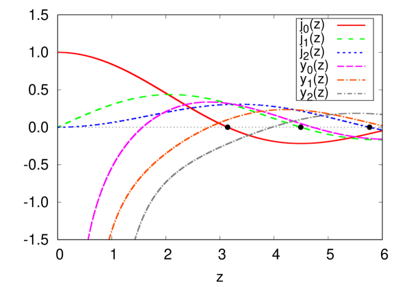
Figure 2: (Color online) Examples of Bessel functions of the first, Eq. (29), and second, Eq. (30), kinds. We plot the first three orders, $l=0,1,2$, using solid (red), dashed (green), short-dashed (blue), long-dashed (magenta), dash-dotted (orange), and short-dash-dotted (gray) curves to denote $j_{0}$, $j_{1}$, $j_{2}$, $y_{0}$, $y_{1}$, and $y_{2}$, respectively. The (black) solid circles denote the Bessel zeros $z_{10}$, $z_{11}$, and $z_{12}$. Notice that the Bessel functions of the first kind are well-behaved near the origin, whereas the ones of the second kind diverge.

To obtain the energy levels, we need to apply the boundary conditions of our problem into the solutions of Eq. (28). The wave function must be well-behaved at the origin, hence the spherical Bessel functions of the second kind are not acceptable solutions. Also, it cannot have any kinks at the origin, thus $R_{nl}^{\prime}(0)=0$, which is satisfied by the spherical Bessel functions of the first kind. The boundary condition at $r=a$, where the wave function must vanish, gives us the condition $R_{nl}(ka)=0$. Denoting the $n$-th zero of $j_{l}$ by $z_{nl}$, we have $k=z_{nl}/a$, and the energy levels are

$$\varepsilon_{nl}=\frac{\hbar^{2}}{2M}\frac{z^{2}_{nl}}{a^{2}}.$$ (31)

Thus our problem of determining the energy levels for this system reduces to finding the zeros of Bessel functions of the first kind. In Fig. 2 we show the first zeros for $l=0,1,2$. Although there are no analytical expressions for the $z_{nl}$, we can easily find them numerically Hamming (2012). As we found out in Sec. IV, each of these levels has a $2l+1$ degeneracy corresponding to the angular part of the solution.

Now that we determined the energy levels and their degeneracies, the cumulative state number function $\mathcal{N}(\varepsilon)$, Sec. II.3, can be easily calculated. The steps can be summarized as

1. Choose a maximum value of the energy $\varepsilon_{m}$, or equivalently, a maximum value of $k$, $k_{m}=\sqrt{2M\varepsilon_{m}}/\hbar$.

2. Choose a number of bins, $n_{\rm bin}$. Each bin will correspond to an energy interval of width $\hbar^{2}k_{m}^{2}/(2Mn_{\rm bin})$, centered at $\varepsilon_{\rm bin}$.

3. Find all the $z_{nl}\leqslant k_{m}a$. For each one of the zeros, we consider its $2l+1$ degenerescence in the corresponding bin.

4. For each of the bins, add the value of all the preceding bins to it. This guarantees that we are counting the total number of states with energy $\varepsilon\leqslant\varepsilon_{\rm bin}$, as required by the definition of $\mathcal{N}(\varepsilon)$.

We used this procedure to calculate the cumulative state number and density of states of a spherical box, Fig. 3, which we compared with the predictions of the semi-classical approximation, Eqs. (11) and (12). Two main features are illustrated in this plot. The cumulative state function we obtained from our quantum mechanical calculation is slightly below the semi-classical approximation result, which means that thermodynamical quantities differ in these two schemes, as we will see in Sec. VII.1. Another feature is that the numerical calculation of the cumulative state number is smoother than the respective density of states, as discussed in Sec. II.2.

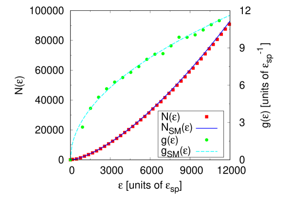
Figure 3: (Color online) Cumulative state number and density of states of a spherical box as a function of the energy. The points correspond to our numerical calculations, (red) squares denote the cumulative state number $\mathcal{N}(\varepsilon)$, while (green) circles represent the density of states $g(\varepsilon)$. The curves are given by the semi-classical approximation, the solid (blue) curve corresponds to Eq. (11), $\mathcal{N}_{\rm SC}(\varepsilon)$, and the dashed (cyan) curve to Eq. (12), $g_{\rm SC}(\varepsilon)$. The energies are expressed in terms of the energy unit $\varepsilon_{\rm sp}=\hbar^{2}/(2Ma^{2})$. Notice that the $\mathcal{N}(\varepsilon)$ from our quantum calculation is slightly lower than the expected result from the semi-classical approximation. Another feature this plot illustrates is that numerical calculations of the cumulative state number are smoother than the density of states.

The energy levels of the sphere, Eq. (31), can be written as $\varepsilon_{nl}=\varepsilon_{sp}(z_{nl})^{2}$, with $\varepsilon_{\rm sp}=\hbar^{2}/(2Ma^{2})$. That is why we chose to express energy dependent quantities in energy units of $\varepsilon_{\rm sp}$. This has the advantage of making our results system-independent, in the sense that the calculation is the same for different values of the mass of the atoms $M$ and radius of the sphere $a$. Once values of $M$ and $a$ are chosen, then the energy is rescaled by the value of $\varepsilon_{\rm sp}$, accordingly.

Equation (8) gives us the cumulative state number for a $D$-dimensional system. In particular, for the 3D sphere we can rewrite the equation as

$$\mathcal{N}(\varepsilon)=C_{sp}\varepsilon^{\alpha},$$ (32)

where

$$C_{sp}=\frac{2}{9\pi\varepsilon_{sp}^{3/2}}\text{ and }\alpha=\frac{3}{2}.$$ (33)

A close inspection of Fig. 3 reveals that the relative difference between our numerical results and the semi-classical approximation is of the order of 1% for $\varepsilon=10^{4}\varepsilon_{\rm sp}$. If we increase the energy cutoff, beyond the range of the graph, then it would drop to $\approx 0.1$% for $\varepsilon=1.5$ $10^{5}$ $\varepsilon_{\rm sp}$, and the difference between them continues to decrease as we increase the energy cutoff. This is in agreement with the findings of Sec. II.3, for large energy values the two expressions should coincide.

However, this difference impacts the behavior of the system for small energies. In order to quantify this deviation, we took the logarithm of Eq. (32),

$$\ln\mathcal{N}(\varepsilon)=\ln C_{\rm sp}+\alpha\ln\varepsilon.$$ (34)

The plot of $\ln\mathcal{N}$ vs. $\ln\varepsilon$ graph is simply a line, with angular coefficient $\alpha$ and linear coefficient $\ln C_{\rm sp}$. In Fig. 4 we show the angular and linear coefficients for the $\varepsilon\leqslant 12000\varepsilon_{\rm sp}$ energy range. Each of the points $\{\varepsilon_{i}\}$ correspond to a linear fit of our data, up to that energy, to Eq. (34). We can see that increasing the energy cutoff yields coefficients that are much closer to the expected high energy limits.

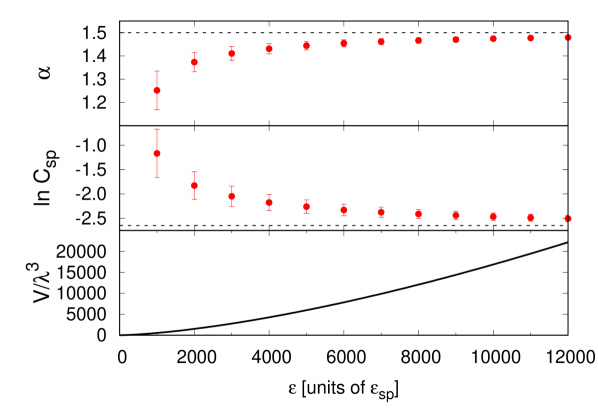
Figure 4: (Color online) Angular coefficient $\alpha$, linear coefficient $\ln C_{\rm sp}$, and volume over wavelength cubed $V/\lambda^{3}$, for a spherical box as a function of the energy. The dashed lines correspond to the classical (high energy) limit of $\alpha=3/2$ and $\ln C_{\rm sp}=\ln(2/(9\pi\varepsilon_{\rm sp}^{3/2}))$. The bottom panel illustrates Weyl’s theorem: we fixed the volume $V$ and varied the wavelength $\lambda=2\pi/k$. Larger values of $V/\lambda^{3}$ correspond to angular and linear coefficients that are closer to the expected classical limit.

Another feature that we chose to illustrate in Fig. 4 is Weyl’s theorem. The bottom panel shows, for a fixed volume, the ratio $V/\lambda^{3}$, which increases with the energy. As we can see, as the ratio increases, the closer the angular and linear coefficients become to the high energy limit given by Eq. (33). This is consistent with what we presented in Sec. II.5, as the energy of the particle increases, it becomes insensitive to the shape of the sphere, and its cumulative state number approaches the expression we derived for a rigid box.

VI Thick shell

Let us consider the external potential

$$V(r)=\begin{cases}0\phantom{+\infty}\text{ if }a<r<b,\\ +\infty\phantom{0}\text{ otherwise}.\end{cases}$$ (35)

We refer to this potential as a thick shell because a shell is a two-dimensional object, whereas the potential of Eq. (35) traps the particle in a spherically symmetric region with thickness $\delta=b-a$. Equation (23) for the region $a<r<b$ is the same as Eq. (27), which means that linear combinations of the spherical Bessel functions of the first and second kinds, Eqs. (29) and (30), are also solutions to this equation.

However, the boundary conditions are different from the ones employed in the spherical box, Sec. V, $R_{nl}(r=a)=R_{nl}(r=b)=0$. This yields the system of linear equations

$$Aj_{l}(ka)+By_{l}(ka) = 0,$$

$$Aj_{l}(kb)+By_{l}(kb) = 0,$$ (36)

where $A$ and $B$ are constants that need to be determined. The non-trivial solution requires

$$j_{l}(ka)y_{l}(kb)-j_{l}(kb)y_{l}(ka)=0.$$ (37)

Again, our problem reduces to finding the values of $k$ that satisfy the equation above. We employ numerical methods to find them Hamming (2012).

Unlike the spherical box, where the only length scale of the problem is the radius of the sphere, there are two length scales present in the thick shell: the radii $a$ and $b$ or, equivalently, the thickness $\delta$ and the center of the sphere $R=(a+b)/2$. This means that the approach we employed in the case of the sphere, of defining quantities in energy units of $\varepsilon_{\rm sp}$, will not work here. Hence, the parameter choice was made keeping in mind typical values for the number density employed in trapped BECs Dalfovo et al. (1999), which yields the range between 10 and 15 $\mu m$ for $a$ and $b$.

In Fig. 5 we plot the cumulative state number for the spherical box and the thick shell. For both sets of internal radii $a=$ 10 $\mu$m and $a=$ 14 $\mu$m, with the external radius $b=$ 15 $\mu$m fixed, our (quantum) numerical calculations yield slightly lower values if compared to the semi-classical approximation of Eq. (11). Again it is possible to see the manifestation of Weyl’s theorem. The spherical box with radius $a=(15^{3}-14^{3})^{1/3}\mu$m $\approx 8.6$ $\mu$m and the thick shell with $a=$ 14 $\mu$m and $b=$ 15 $\mu$m have the same volumes, however totally different shapes. Their cumulative state number function presents a small deviation, which increases with the decreasing of the trap volume.

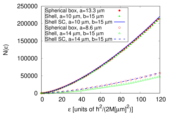
Figure 5: (Color online) Cumulative state number for the spherical box and thick shell as a function of the energy. The points correspond to our numerical calculations, and the curves to the semi-classical approximation of Eq. (11). The open (red) circles correspond to the spherical box with radius $a=(15^{3}-14^{3})^{1/3}\mu$m $\approx 8.6$ $\mu$m, which was chosen such that the sphere has the same volume as the thick shell with $a=$ 14 $\mu$m and $b=$ 15 $\mu$m, open (green) triangles. We also plot the cumulative state number for a different internal radius, $a=$ 10 $\mu$m, while keeping the external radius fixed at $b=$ 15 $\mu$m, denoted by the solid (green) triangles, and the spherical box (same volume) of radius $\approx 13.3$ $\mu$m solid (red) circles. The semi-classical approximations for $a=$ 10 $\mu$m and $a=$ 14 $\mu$m, solid and dashed (blue) curves respectively, are slightly above the corresponding quantum calculations.

In order to quantify this difference, we proceeded analogously to what we did in Sec. V. The logarithm of the state number function is given by

$$\ln N(\varepsilon)=\ln C_{\rm sh}+\alpha\ln\varepsilon,$$ (38)

where the high energy limit corresponds to $\alpha=3/2$ and $C_{\rm sh}=[2(b^{3}-a^{3})/(9\pi)](2M/\hbar^{2})^{3/2}$. In Fig. 6 we show the linear fit of our data to Eq. (38). It is possible to see that larger values of the thickness yield angular and linear coefficients that are closer to the high energy limit, as expected. We should note that the angular coefficients $\alpha$ are slightly lower than 3/2 for $\delta\gtrsim$ 8 $\mu$m. This is explained by the fact that increasing the volume, or the energy cutoff, makes the angular coefficient approach 3/2 from below, as was the case with the spherical box, see Fig. 4. For the range $\delta\lesssim$ 8 $\mu$m there is competition between the energy cutoff, the change in volume, and also the change in dimensionality, as $\delta/R\ll 1$.

We also verified Weyl’s theorem by varying both the volume $V$ and the wavelength $\lambda$ and calculating the ratio $V/\lambda^{3}$. For a fixed value of the thickness (for example $\delta$= 1 $\mu$m) the larger the ratio, the closer the angular and linear coefficients are to the expected limits.

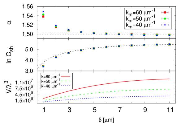
Figure 6: (Color online) Angular coefficient $\alpha$, linear coefficient $\ln C_{\rm sh}$, and the ratio $V/\lambda^{3}$, for a thick shell as a function of the thickness $\delta$. The external radius was kept fixed at 15 $\mu$m, while the internal radius $a$ was varied between 4 and 14 $\mu$m. We plot the data points corresponding to our numerical calculations for the cutoffs $k_{m}=$ 40, 50, and 60 $\mu$m^-1, (blue) triangles, (green) circles, and (red) squares, respectively. The dashed lines correspond to the classical (high energy) limit of $\alpha=3/2$ and $\ln C_{\rm sh}=\ln[2(b^{3}-a^{3})/(9\pi)](2M/\hbar^{2})^{3/2}$. The bottom panel illustrates Weyl’s theorem: for different values of $k$ we calculated the ratio $V/\lambda^{3}$, with $\lambda=2\pi/k$. We show the ratios for $k=$ 40, 50, and 60 $\mu$m^-1, (blue) short-dashed, (green) dashed, and (red) solid curve, respectively. Larger values of $V/\lambda^{3}$ correspond to angular and linear coefficients that are closer to the expected classical limit as illustrated, for example, by the values of $\alpha$ for $\delta=$ 1 $\mu$m.

VII Critical temperature

VII.1 Three-dimensional systems

Finally, we have all the ingredients to calculate the critical temperature for Bose-Einstein condensation in the spherical box and thick shell traps. The semi-classical calculation corresponds to Eq. (18) with the pertinent volume. We assume $N=10^{5}$ particles, which is consistent with cold gases in harmonic traps Dalfovo et al. (1999). We considered 3 atomic species which are commonly employed in cold atoms experiments: ²³Na, ⁸⁷Rb, and ¹³³Cs. We disregard the interaction between the atoms, i.e., we are assuming an ideal Bose gas. Their atomic masses are available in Ref. Wang et al. (2017) in unified atomic mass units. A useful reference for physical constants is the “2014 CODATA (Committee on Data for Science and Technology) recommended values”, which is generally recognized worldwide for use in all fields of science and technology Mohr et al. (2016). We used their values for atomic units [u c²], $\hbar$c [eV $\mu$m], and $k_{B}$ [eV/K] to compute Eq. (18).

We present our results for the semi-classical values of $T_{c}$ in Fig. 7 as open symbols. Equation (18) shows that $T_{c}$ is inversely proportional to the atomic mass $M$ hence, for a given geometry, ²³Na displays the highest critical temperature and ¹³³Cs the lowest. We should also note that the spherical trap with $a=(15^{3}-14^{3})^{1/3}\mu$m $\approx 8.6$ $\mu$m and the thick shell with $a=$ 14 $\mu$m and $b=$ 15 $\mu$m have the same volumes, thus their critical temperatures are the same in the semi-classical scheme.

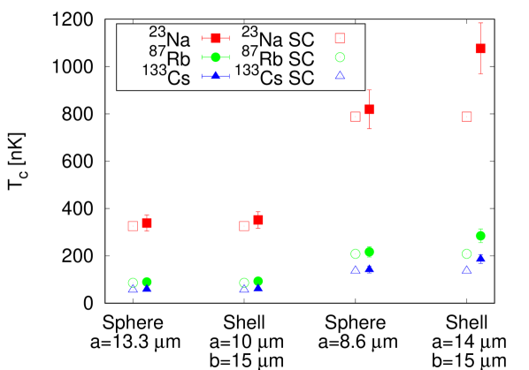
Figure 7: (Color online) Critical temperature for Bose-Einstein condensation for different atomic species in spherically symmetric traps. Open symbols stand for the semi-classical approximation of Eq. (18), while solid symbols correspond to our numerical calculations. We denote ²³Na, ⁸⁷Rb, and ¹³³Cs by (red) squares, (green) circles, and (blue) triangles, respectively. Note that the spherical trap with $a=(15^{3}-14^{3})^{1/3}\mu$m $\approx 8.6$ $\mu$m and the thick shell with $a=$ 14 $\mu$m and $b=$ 15 $\mu$m contain the same volumes, thus their critical temperatures are the same in the semi-classical approximation. The same is true for the sphere with $a=(15^{3}-10^{3})^{1/3}\mu$m $\approx 13.3$ $\mu$m and the thick shell with $a=$ 10 $\mu$m and $b=$ 15 $\mu$m.

We also calculated the critical temperature using our numerical calculations of the density of states $g(\varepsilon)$ and Eq. (16). We show the results in Fig. 7 using solid symbols. Although many of the results are within the error bars (the computation of the density of states introduces numerical errors), our quantum results are consistently larger than the semi-classical ones, mainly when we consider the thinner shell case. This is in agreement with our findings in Secs. V and VI, where our cumulative state number functions are smaller than the semi-classical approximation.

VII.2 From 3D to 2D

As the thickness $\delta$ of the shell approaches zero, we expect the behavior of the system to transition from 3D to 2D. Let us see what happens when the external radius $b=a+\delta$ goes to the internal radius $a$, $\delta\to 0$. We can perform a Taylor expansion of the spherical Bessel functions, Eqs. (29) and (30),

$$f_{l}(k(a+\delta))=f_{l}(ka)$$

$$+\frac{\delta}{2}\left(kf_{l-1}(ka)-\frac{f_{l}(ka)}{a+\delta}-kf_{l+1}(ka)\right)+\mathcal{O}(\delta^{2}),$$ (39)

where $f_{l}$ can denote either $j_{l}$ or $y_{l}$, and we used the property $df_{l}(z)/dz=(1/2)(f_{l-1}(z)-f_{l}(z)/z+f_{l+1}(z))$. Substituting this into Eq. (37) yields

$$k\delta\left(j_{l}(ka)y_{l-1}(ka)-j_{l-1}(ka)y_{l}(ka)\right)=0.$$ (40)

Another property of the spherical functions is Abramowitz and Stegun (2012)

$$j_{l}(z)y_{l-1}(z)-j_{l-1}(z)y_{l}(z)=\frac{1}{z^{2}}.$$ (41)

Putting everything together we have,

$$\left(\frac{\delta}{a}\right)\left(\frac{1}{ka}\right)=0.$$ (42)

This should not be surprising: as $\delta/a$ goes to zero we need an infinite amount of energy, here represented by $ka\to\infty$, to excite the radial degree of freedom.

The proper way to determine the energy levels of a truly two-dimensional shell is to start from the 2D Schrödinger equation. However, we already saw in Sec. IV that the spherical harmonics are the solutions for this case,

$$-\frac{\hbar^{2}}{2M}\nabla^{2}Y_{lm}=\frac{\hbar^{2}}{2Ma^{2}}l(l+1),$$ (43)

from where we get the energy levels,

$$\varepsilon_{l}=\varepsilon_{\rm sp}l(l+1),$$ (44)

with degeneracy $2l+1$, as argued in Sec. IV.

The total number of bosons is given by Eq. (15),

$$N=\sum_{l=0}^{+\infty}\frac{2l+1}{\exp[(\varepsilon_{l}-\mu)/(k_{B}T)]-1}.$$ (45)

In the Bose-Einstein condensate we can set $\mu=0$ and we can separate the number of atoms in the lowest energy state $N_{0}$,

$$N=N_{0}+\sum_{l=1}^{+\infty}\frac{2l+1}{\exp[\varepsilon_{l}/(k_{B}T)]-1}.$$ (46)

The critical temperature corresponds to one above which $N_{0}=0$. Within a semi-classical approximation , we can take $\sum_{l=1}^{+\infty}\to\int_{1}^{+\infty}dl$, yielding

$$N=N_{0}+\frac{4\pi a^{2}Mk_{B}T}{2\pi\hbar^{2}}\times$$

$$\left(\frac{\hbar^{2}}{Ma^{2}k_{B}T}-\ln\left(\exp\left[\frac{\hbar^{2}}{(ma^{2}k_{B}T)}\right]-1\right)\right).$$ (47)

In the low-temperature limit, the second term on the right hand side vanishes and $N$ coincides with $N_{0}$. At $T_{c}$, $N_{0}$ must be zero, hence we have the implicit equation for $T_{c}$:

$$T_{c}=\frac{\frac{2\pi\hbar^{2}}{Mk_{B}}\left(\frac{N}{A}\right)}{\left(\frac{\hbar^{2}}{Ma^{2}k_{B}T_{c}}-\ln\left(\exp[\hbar^{2}/(ma^{2}k_{B}T_{c})]-1\right)\right)},$$ (48)

where $A=4\pi a^{2}$ is the area of the shell. We used Eq. (48) to compute the critical temperature for 2D shells of radii compatible with the thick shells we studied in Sec. VII.1. For example, the thick shell with internal radius 10 $\mu$m and external radius 15 $\mu$m, was compared with a shell at 12.5 $\mu$m. We found that the critical temperature of the shells is 1.5 to 2 times larger than the one for the thick shells. This means that our thick shells are far away from being two-dimensional systems.

It is worth mentioning that the semi-classical approximation for the two-dimensional shell, the 2D equivalent of Eq. (12), does not give a finite critical temperature for Bose-Einstein condensation, with $T_{c}$ being zero in the limit of a plane geometry. It is the curvature of the spherical shell that allows a finite critical temperature.

VIII Summary

One of the main goals of this work was to compare and contrast the semi-classical approximation for the density of states, and cumulative state number, with quantum mechanical calculations. We found differences at the low-energy regime, which is the most relevant for cold atomic gases, which impact the thermodynamical properties of these systems. We also verified the manifestation of Weyl’s theorem by comparing the same geometry with different energy regimes, or the spherical box and thick shell with the same volume.

The critical temperature range we obtained, see Fig. 7, is compatible with current cold atom experiments. Indeed, systems with thick shell trapping potentials, usually called bubble traps, are being investigated theoretically Padavić et al. (2017) and experimentally Elliott et al. (2018); Becker et al. (2018).

In Sec. VII.2 we discuss the effects of reducing the dimensionality of the system of interest from 3D to 2D, which is what happens when the thickness of the shell goes to zero. The change of dimensionality is an active topic of research in cold atoms Görlitz et al. (2001); Bloch et al. (2008).

We consider the calculations presented in this paper good introductory examples for numerical computations in statistical physics. Understandably, undergraduate physics courses tend to focus on analytically solvable problems. However it is of paramount importance that students learn to perform numerical calculations, since analytical solutions are very rare in active research areas.

This manuscript can also be used as a starting point to study trapping geometries with other symmetries. For example, cylindrical geometries are useful in the study of vortex lines in cold gases Vitiello et al. (1996); Madeira et al. (2016, 2019). In two-dimensions, disks can be used to investigate point-like vortices Ortiz and Ceperley (1995); Giorgini et al. (1996); Madeira et al. (2017).

Appendix A Critical temperature in $D$-dimensions

In this appendix we calculate the critical temperature for a $D$-dimensional condensate. First, let us consider the integral,

$$I(p)=\int_{0}^{\infty}dx\frac{x^{p-1}}{e^{x}-1}=\int_{0}^{\infty}dx\ e^{-x}(1-e^{-x})^{-1}x^{p-1}$$

$$=\int_{0}^{\infty}dx\ e^{-x}\left[\sum_{k=0}^{\infty}(e^{-x})^{k}\right]x^{p-1}$$

$$=\sum_{k=0}^{\infty}\int_{0}^{\infty}dx\ e^{-x(k+1)}x^{p-1}.$$ (49)

Integrals of this form are often called Bose integrals. Substituting $y=x(k+1)$,

$$I(p)=\sum_{k=0}^{\infty}\frac{1}{(k+1)^{p}}\int_{0}^{\infty}dy\ e^{-y}y^{p-1}$$

$$=\Gamma(p)\sum_{k=0}^{\infty}\frac{1}{(k+1)^{p}}=\Gamma(p)\sum_{k=1}^{\infty}\frac{1}{k^{p}}=\Gamma(p)\zeta(p),$$ (50)

where $\Gamma$ is the gamma function and $\zeta$ is the Riemann zeta function.

Equation (9) gives us the expression for the $D$-dimensional density of states, which can be rewritten in the form $g_{D}(\varepsilon)=C_{D}V\varepsilon^{D/2-1}$, with $C_{D}=C_{D}^{\prime}D/(2^{D+1}\varepsilon_{0}^{D/2}V)$, for brevity. For this density of states,

$$N=C_{D}V\int_{0}^{\infty}d\varepsilon\frac{\varepsilon^{D/2-1}}{e^{\beta_{c}\varepsilon}-1}.$$ (51)

Let us perform the substitution $x=\beta_{c}\varepsilon$,

$$N=\frac{C_{D}V}{\beta_{c}^{D/2}}\int_{0}^{\infty}dx\frac{x^{D/2-1}}{e^{x}-1}.$$ (52)

Using the result of Eq. (A),

$$N=\frac{C_{D}V}{\beta_{c}^{D/2}}\Gamma\left(\frac{D}{2}\right)\zeta\left(\frac{D}{2}\right).$$ (53)

Solving for the critical temperature yields

$$T_{c}=\frac{1}{k_{B}}\left[\frac{1}{C_{D}\Gamma(D/2)\zeta(D/2)}\frac{N}{V}\right]^{2/D}.$$ (54)

If we set $D=3$, this equation agrees with Eq. (18), as it should.

References

- Bose (1924) Bose, Zeitschrift für Physik 26, 178 (1924).
- Pethick and Smith (2002) C. Pethick and H. Smith, Bose-Einstein Condensation in Dilute Gases (Cambridge University Press, 2002).
- Anderson et al. (1995) M. H. Anderson, J. R. Ensher, M. R. Matthews, C. E. Wieman, and E. A. Cornell, Science 269, 198 (1995), http://science.sciencemag.org/content/269/5221/198.full.pdf .
- Bradley et al. (1995) C. C. Bradley, C. A. Sackett, J. J. Tollett, and R. G. Hulet, Phys. Rev. Lett. 75, 1687 (1995).
- Davis et al. (1995) K. B. Davis, M. O. Mewes, M. R. Andrews, N. J. van Druten, D. S. Durfee, D. M. Kurn, and W. Ketterle, Phys. Rev. Lett. 75, 3969 (1995).
- Griffin et al. (1996) A. Griffin, D. Snoke, and S. Stringari, Bose-Einstein Condensation (Cambridge University Press, 1996).
- Ketterle et al. (1999) W. Ketterle, D. S. Durfee, and D. M. Stamper-Kurn, “Making, probing and understanding Bose-Einstein condensates,” (1999), arXiv:cond-mat/9904034 .
- Gaunt et al. (2013) A. L. Gaunt, T. F. Schmidutz, I. Gotlibovych, R. P. Smith, and Z. Hadzibabic, Phys. Rev. Lett. 110, 200406 (2013).
- Zobay and Garraway (2001) O. Zobay and B. M. Garraway, Physical Review Letters 86, 1195 (2001).
- Zobay and Garraway (2004) O. Zobay and B. M. Garraway, Physical Review A 69 (2004), 10.1103/physreva.69.023605.
- Garraway and Perrin (2016) B. M. Garraway and H. Perrin, Journal of Physics B: Atomic, Molecular and Optical Physics 49, 172001 (2016).
- Elliott et al. (2018) E. R. Elliott, M. C. Krutzik, J. R. Williams, R. J. Thompson, and D. C. Aveline, npj Microgravity 4 (2018), 10.1038/s41526-018-0049-9.
- Giorgini et al. (2008) S. Giorgini, L. P. Pitaevskii, and S. Stringari, Rev. Mod. Phys. 80, 1215 (2008).
- Bloch et al. (2008) I. Bloch, J. Dalibard, and W. Zwerger, Rev. Mod. Phys. 80, 885 (2008).
- Mulhall and Moelter (2014) D. Mulhall and M. J. Moelter, American Journal of Physics 82, 665 (2014), https://doi.org/10.1119/1.4867489 .
- Griffiths and Schroeter (2018) D. Griffiths and D. Schroeter, Introduction to Quantum Mechanics (Cambridge University Press, 2018).
- Sommerville (1929) D. Sommerville, An Introduction to the Geometry of N Dimensions (E. P. Dutton, Incorporated, 1929).
- Arfken et al. (2011) G. Arfken, H. Weber, and F. Harris, Mathematical Methods for Physicists: A Comprehensive Guide (Elsevier Science, 2011).
- Bagnato et al. (1987) V. Bagnato, D. E. Pritchard, and D. Kleppner, Phys. Rev. A 35, 4354 (1987).
- Weyl (1912) H. Weyl, Mathematische Annalen 71, 441 (1912).
- Kac (1966) M. Kac, The American Mathematical Monthly 73, 1 (1966).
- Lambert (1968) R. H. Lambert, American Journal of Physics 36, 417 (1968), https://doi.org/10.1119/1.1974552 .
- Salinas (2013) S. Salinas, Introduction to Statistical Physics, Graduate Texts in Contemporary Physics (Springer New York, 2013).
- Abramowitz and Stegun (2012) M. Abramowitz and I. Stegun, Handbook of Mathematical Functions: with Formulas, Graphs, and Mathematical Tables, Dover Books on Mathematics (Dover Publications, 2012).
- Butkov (1968) E. Butkov, Mathematical physics, Addison-Wesley series in advanced physics (Addison-Wesley Pub. Co., 1968).
- Hamming (2012) R. Hamming, Numerical Methods for Scientists and Engineers, Dover Books on Mathematics (Dover Publications, 2012).
- Dalfovo et al. (1999) F. Dalfovo, S. Giorgini, L. P. Pitaevskii, and S. Stringari, Rev. Mod. Phys. 71, 463 (1999).
- Wang et al. (2017) M. Wang, G. Audi, F. G. Kondev, W. Huang, S. Naimi, and X. Xu, Chinese Physics C 41, 030003 (2017).
- Mohr et al. (2016) P. J. Mohr, D. B. Newell, and B. N. Taylor, Rev. Mod. Phys. 88, 035009 (2016).
- Note (1) A. Tononi and L. Salasnich, private communication.
- Padavić et al. (2017) K. Padavić, K. Sun, C. Lannert, and S. Vishveshwara, EPL (Europhysics Letters) 120, 20004 (2017).
- Becker et al. (2018) D. Becker, M. D. Lachmann, S. T. Seidel, H. Ahlers, A. N. Dinkelaker, J. Grosse, O. Hellmig, H. Müntinga, V. Schkolnik, T. Wendrich, A. Wenzlawski, B. Weps, R. Corgier, T. Franz, N. Gaaloul, W. Herr, D. Lüdtke, M. Popp, S. Amri, H. Duncker, M. Erbe, A. Kohfeldt, A. Kubelka-Lange, C. Braxmaier, E. Charron, W. Ertmer, M. Krutzik, C. Lämmerzahl, A. Peters, W. P. Schleich, K. Sengstock, R. Walser, A. Wicht, P. Windpassinger, and E. M. Rasel, Nature 562, 391 (2018).
- Görlitz et al. (2001) A. Görlitz, J. M. Vogels, A. E. Leanhardt, C. Raman, T. L. Gustavson, J. R. Abo-Shaeer, A. P. Chikkatur, S. Gupta, S. Inouye, T. Rosenband, and W. Ketterle, Physical Review Letters 87 (2001), 10.1103/physrevlett.87.130402.
- Vitiello et al. (1996) S. A. Vitiello, L. Reatto, G. V. Chester, and M. H. Kalos, Phys. Rev. B 54, 1205 (1996).
- Madeira et al. (2016) L. Madeira, S. A. Vitiello, S. Gandolfi, and K. E. Schmidt, Phys. Rev. A 93, 043604 (2016).
- Madeira et al. (2019) L. Madeira, S. Gandolfi, K. E. Schmidt, and V. S. Bagnato, “Vortices in low-density neutron matter and cold Fermi gases,” (2019), arXiv:1903.06724 .
- Ortiz and Ceperley (1995) G. Ortiz and D. M. Ceperley, Phys. Rev. Lett. 75, 4642 (1995).
- Giorgini et al. (1996) S. Giorgini, J. Boronat, and J. Casulleras, Phys. Rev. Lett. 77, 2754 (1996).
- Madeira et al. (2017) L. Madeira, S. Gandolfi, and K. E. Schmidt, Phys. Rev. A 95, 053603 (2017).