Fundamental limits to radiative heat transfer: the limited role of nanostructuring in the near-field

Abstract

In a complementary article Molesky et al. (2019), we exploited algebraic properties of Maxwell’s equations and fundamental principles such as electromagnetic reciprocity and passivity, to derive fundamental limits to radiative heat transfer applicable in near- through far-field regimes. The limits depend on the choice of material susceptibilities and bounding surfaces enclosing arbitrarily shaped objects. In this article, we apply these bounds to two different geometric configurations of interest, namely dipolar particles or extended structures of infinite area in the near field of one another, and compare these predictions to prior limits. We find that while near-field radiative heat transfer between dipolar particles can saturate purely geometric “Landauer” limits, bounds on extended structures cannot, instead growing much more slowly with respect to a material response figure of merit, an “inverse resistivity” for metals, due to the deleterious effects of multiple scattering; nanostructuring is unable to overcome these limits, which can be practically reached by planar media at the surface polariton condition.

Radiative heat transfer (RHT) between two bodies may be written as a frequency integral of the form

$$P=\int_{0}^{\infty}[\Pi(\omega,T_{\mathrm{B}})-\Pi(\omega,T_{\mathrm{A}})]\Phi(\omega)\leavevmode\nobreak\ \mathrm{d}\omega$$ (1)

where $\Pi(\omega,T)$ is the Planck function (and it has been assumed, without loss of generality, that $T_{\mathrm{B}}>T_{\mathrm{A}}$ so $P>0$), and $\Phi(\omega)$ a dimensionless spectrum of energy transfer. RHT between two objects sufficiently separated in space follows the Planck blackbody law, but in the near-field where separations are smaller than the characteristic thermal wavelength of radiation, contributions to RHT from evanescent modes will dominate, allowing $\Phi(\omega)$ to exceed the far-field blackbody limits by orders of magnitude. Moreover, because the Planck function decays exponentially with frequency, judicious choice of materials and nanostructured geometries can shift resonances in $\Phi$ to lower (especially infrared) frequencies, allowing observation of even larger integrated RHT powers Volokitin and Persson (2001); Domingues et al. (2005); Volokitin and Persson (2007); Song et al. (2015). However, after accounting for the effects of such frequency shifts, the degree to which the spectrum $\Phi$ at a given frequency can be enhanced remains an open question. The inability of trial-and-error explorations and optimization procedures Jin et al. (2017); Fernández-Hurtado et al. (2017) to saturate prior bounds on $\Phi$ based on modal analyses Pendry (1999); Bimonte (2009); Biehs et al. (2010); Ben-Abdallah and Joulain (2010) or energy conservation Miller et al. (2015) suggests that these prior bounds may be too loose.

In a complementary article Molesky et al. (2019), we derived new bounds that simultaneously account for material and geometric constraints as well as multiple scattering effects. These bounds, valid from the near- through far-field regimes, incorporate the dependence of the optimal modal response of each object on the other while simultaneously being constrained by passivity considerations in isolation. They depend on a general material response factor (“inverse resistivity” for metals) Miller et al. (2015),

$$\zeta=\frac{|\chi|^{2}}{\operatorname{Im}(\chi)},$$ (2)

without making explicit reference to specific frequencies or dispersion models, and are domain monotonic, increasing with object volumes independently of their shapes. Consequently, our bounds are applicable at all length scales, from quasistatic to ray optics regimes, do not suffer from unphysical divergences with respect to vanishing material dissipation or object sizes Miller et al. (2015), and can be interpreted independently of specific object shapes.

In this article, we apply the aforementioned bounds on $\Phi$ to two geometric configurations of practical interest, comparing predictions to prior bounds based on energy conservation Miller et al. (2015), applicable only in the quasistatic regime, or Landauer-like modal summations Pendry (1999); Bimonte (2009); Biehs et al. (2010); Ben-Abdallah and Joulain (2010), applicable only in the ray optics regime. Specifically, we consider limits on RHT between dipolar particles as well as extended structures of infinite area and arbitrary shapes restricted to the near field. We find that our exact bound for dipolar particles is able to reach Landauer limits when $\zeta$ exceeds a certain threshold; in contrast, bounds that neglect losses due to multiple scattering grossly overestimate possible material enhancements, diverging with increasing $\zeta$. For extended structures, we find that the bound grows only weakly (logarithmically) with respect to $\zeta$, making the neglect of multiple scattering even more apparent. Fundamentally, previous limits Miller et al. (2015) were based on a Born approximation which, in analogy with Kirchhoff’s law Volokitin and Persson (2001, 2007), assumed that thermal fields produced within a given body in isolation can be perfectly absorbed by others in proximity. This explains the aforementioned performance gap: the combination of resonant absorption and multiple scattering hampers rather than helps NFRHT, and the previous bounds cannot capture this trade-off. Finally, we discuss practical implications and design guidelines for structures enhancing NFRHT.

Bound Formula $\begin{array}[]{cc}\text{Material}&\\ \text{factor}\end{array}$ $\begin{array}[]{cc}\text{Multiple}&\\ \text{scattering}\end{array}$ $\Phi_{\mathrm{opt}}$ $\begin{array}[]{lcl}&&\sum_{i}\frac{1}{2\pi}\Theta(\zeta_{\mathrm{A}}\zeta_{\mathrm{B}}g_{i}^{2}-1)\\ &+&\sum_{i}\frac{2}{\pi}\frac{\zeta_{\mathrm{A}}\zeta_{\mathrm{B}}g_{i}^{2}}{(1+\zeta_{\mathrm{A}}\zeta_{\mathrm{B}}g_{i}^{2})^{2}}\Theta(1-\zeta_{\mathrm{A}}\zeta_{\mathrm{B}}g_{i}^{2})\end{array}$ Yes Yes $\Phi_{\mathrm{Born}}$ $\sum_{i}\frac{2}{\pi}\zeta_{\mathrm{A}}\zeta_{\mathrm{B}}g_{i}^{2}$ Yes No $\Phi_{\mathrm{L}}$ $\sum_{i}\frac{1}{2\pi}$ No No $\Phi_{\mathrm{sc}}$ $\sum_{i}\frac{2}{\pi}\frac{\zeta_{\mathrm{A}}\zeta_{\mathrm{B}}g_{i}^{2}}{(1+\zeta_{\mathrm{A}}\zeta_{\mathrm{B}}g_{i}^{2})^{2}}$ Yes Yes

Table 1: Summary of various bounds on NFRHT. $\Phi_{\mathrm{opt}}$ captures multiple scattering and geometric constraints via the singular values $\{g_{i}\}$ of the vacuum Green’s function $\mathbb{G}^{\mathrm{vac}}_{\mathrm{BA}}$, and material constraints via the response factors $\zeta_{p}=\frac{|\chi_{p}|^{2}}{\operatorname{Im}(\chi_{p})}$ for $p=\{\mathrm{A},\mathrm{B}\}$. $\Theta$ is the Heaviside step function. As described in the main text, restricted versions of $\Phi_{\mathrm{opt}}$ each capture different facets of this bound.

General bounds.—We now briefly recapitulate the bounds on RHT between bodies A and B derived in Molesky et al. (2019) and describe their salient features; readers may follow Molesky et al. (2019) for more technical details. These bounds are derived for bodies $p\in\{\mathrm{A},\mathrm{B}\}$ with arbitrary homogeneous local isotropic susceptibilities $\chi_{p}$ and arbitrary shape and size. They depend on material constraints, particularly passivity (nonnegativity of far-field scattering by each object in isolation and in the presence of the other), encoded in the response factors $\zeta_{p}=|\chi_{p}|^{2}/\operatorname{Im}(\chi_{p})$, and on geometric constraints encoded in the off-diagonal vacuum Maxwell Green’s function $\mathbb{G}^{\mathrm{vac}}_{\mathrm{BA}}$, which solves $[(c/\omega)^{2}\nabla\times(\nabla\times)-\mathbb{I}]\mathbb{G}^{\mathrm{vac}}=\mathbb{I}$. In particular, the bounds rest on the singular values $\{g_{i}\}$ obtained from a singular-value decomposition,

$$\mathbb{G}^{\mathrm{vac}}_{\mathrm{BA}}=\sum_{i}g_{i}|\mathbf{b}_{i}\rangle\langle\mathbf{a}_{i}|,$$ (3)

where $|\mathbf{a}_{i}\rangle$ and $|\mathbf{b}_{i}\rangle$ are the corresponding right and left singular vectors, respectively. A key property of this expansion is that the singular values of $\mathbb{G}^{\mathrm{vac}}_{\mathrm{BA}}$ are domain-monotonic, increasing with increasing domain volume.

We list the relevant bounds in Table 1. The main results of this paper rely on the upper bound $\Phi_{\mathrm{opt}}$, which we refer to as an “exact bound” in that it is valid from the near- through far-field regimes, though below we focus only on near-field effects. $\Phi_{\mathrm{opt}}$ is domain monotonic in that it always increases with increasing object volumes, and this comes from the domain monotonicity of $g_{i}$. Therefore, one can choose to evaluate the bound in a domain of high symmetry enclosing the objects of interest, representing a fundamental geometric constraint in analogy and in combination with material constraints imposed by a specific choice of $\zeta_{p}$.

The expression for $\Phi_{\mathrm{opt}}$ makes clear that optimal heat transfer is achievable if the modes of the response of each body coincide with the modes of the vacuum Green’s function $\mathbb{G}^{\mathrm{vac}}_{\mathrm{BA}}$. Additionally, for each channel $i$, each term may be physically interpreted as follows. The first term $\frac{1}{2\pi}$ corresponds to the Landauer limit for that channel, which is the maximum possible contribution to $\Phi$ for a given channel Datta (1995); Klöckner et al. (2016); Pendry (1999); Bimonte (2009); Biehs et al. (2010); Ben-Abdallah and Joulain (2010); a given channel $i$ attains this only if $\zeta_{\mathrm{A}}\zeta_{\mathrm{B}}g_{i}^{2}\geq 1$, meaning that while channels that efficiently couple electromagnetic fields propagating in vacuum between the two bodies can lead to saturation, channels that do not require instead larger material response factors $\zeta_{p}$. In contrast, the total Landauer bound $\Phi_{\mathrm{L}}$ assumes saturation of every channel $i$ (the first term) regardless of material response or geometric configuration. The second term $\frac{2}{\pi}\frac{\zeta_{\mathrm{A}}\zeta_{\mathrm{B}}g_{i}^{2}}{(1+\zeta_{\mathrm{A}}\zeta_{\mathrm{B}}g_{i}^{2})^{2}}$, which never exceeds the per-channel Landauer limit of $\frac{1}{2\pi}$, corresponds to each body attaining its maximum absorptive response in isolation for the respective incident fields $|\mathbf{a}_{i}\rangle$ and $|\mathbf{b}_{i}\rangle$ for channel $i$ in order to satisfy passivity constraints; the numerator corresponds to the contribution from absorption of each body in isolation, while the denominator captures multiple scattering effects among bodies. In contrast, the “scalar approximation” $\Phi_{\mathrm{sc}}$ assumes that each body exhibits maximal isolated absorption (i.e. uniform or scalar response) corresponding to the second term for every channel $i$; while $\Phi_{\mathrm{sc}}$ includes both material response constraints in the numerator and multiple scattering effects in the denominator, the “Born bound” $\Phi_{\mathrm{Born}}$ further dispenses with the denominator (i.e. multiple scattering effects) entirely for every channel $i$ Miller et al. (2015). In Molesky et al. (2019), we proved that these bounds satisfy the inequalities

$$\Phi_{\mathrm{sc}}\leq\Phi_{\mathrm{opt}}\leq\Phi_{\mathrm{Born}},\Phi_{\mathrm{L}}$$ (4)

regardless of the particular bounding domain, and thus we may compare them for specific topologies of interest.

Dipolar bodies.— We first consider NFRHT between either two dipolar particles [Fig. 1(a)] or a dipolar particle and an extended bulk medium of infinite area and thickness [Fig. 1(b)], enclosed within spherical or semi-infinite bounding domains, as detailed in the appendices. The dipolar limit implies that if $V$ is the volume of a dipolar particle and $d$ is the separation from the other body, then $\frac{V^{1/3}}{d}\ll 1$, and no higher-order particle multipoles should matter. This also implies that there are only 3 degrees of freedom or singular values (i.e. polarizations) and therefore 3 channels of interest, meaning that in either case, we can immediately write the Landauer limit as $\Phi_{\mathrm{L}}=\frac{3}{2\pi}$. As we show in the appendices, in the first case, the quantities $\Phi_{\mathrm{opt}}$, $\Phi_{\mathrm{Born}}$, and $\Phi_{\mathrm{sc}}$ depend only on the combined quantity $\frac{\sqrt{\zeta_{\mathrm{A}}\zeta_{\mathrm{B}}V_{\mathrm{A}}V_{\mathrm{B}}}}{d^{3}}$ where $V_{p}$ is the volume of each dipolar body $p\in\{\mathrm{A},\mathrm{B}\}$, while in the second case, they depend on $\sqrt{\frac{\zeta_{\mathrm{A}}\zeta_{\mathrm{B}}V}{d^{3}}}$ where $V$ is the volume of the one dipolar body.

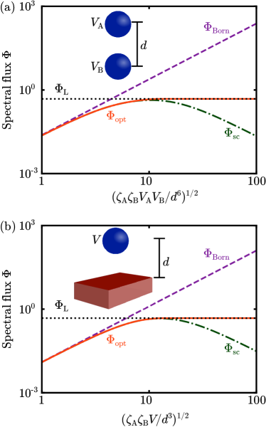
Figure 1: Comparison of $\Phi_{\mathrm{opt}}$ (solid orange) to $\Phi_{\mathrm{L}}$ (dotted black), $\Phi_{\mathrm{Born}}$ (dashed purple), and $\Phi_{\mathrm{sc}}$ (dot-dashed green) for a dipolar body separated by distance $d$ from (a) another dipolar body, in which case both dipolar volumes $V_{\mathrm{A}}$ and $V_{\mathrm{B}}$ are relevant, or (b) an extended structure, in which case only the single dipolar volume $V$ is relevant.

In both cases, the Born bound depends linearly on the product $\zeta_{\mathrm{A}}\zeta_{\mathrm{B}}$, which explains why for increasing material factors (assuming fixed volumes and separations) the bound eventually crosses the Landauer limits. By contrast, $\Phi_{\mathrm{opt}}$ will never cross or exceed either Landauer or Born bounds, while hugging the latter from below and increasing monotonically toward $\Phi_{\mathrm{L}}$ with increasing material factors (e.g. small dissipation). We note that whether the dipolar particle is near another or an extended structure, the smallest two singular values of $\mathbb{G}^{\mathrm{vac}}_{\mathrm{AB}}$ are equal to each other and correspond to the two axes perpendicular to the line of separation, while the largest singular value is larger than the smaller two by different factors depending on the particular case. This dependence therefore implies that for the Landauer bounds to be saturated, the optimal net response of each body cannot be isotropic, even though the underlying susceptibilities are assumed to be isotropic; the optimal dipole should instead arise for an oblate ellipsoidal shape whose aspect ratio is a function of $g_{\max}/g_{\min}$, while the optimal extended structure (assuming an isotropic particle) should be textured in order to break homogeneity. The scalar approximation in each case hugs $\Phi_{\mathrm{opt}}$ from below up until it smoothly reaches a peak, and then decays as a power law thereafter. The peak value of $\Phi_{\mathrm{sc}}$ is within 10% of the Landauer bound in each case, suggesting that for susceptibilities and frequencies chosen to give an appropriate value of $\zeta_{\mathrm{A}}\zeta_{\mathrm{B}}$, the limits can practically be reached by isotropic spherical dipoles and thick planar films; we note that the surface polariton condition is $\operatorname{Re}(1/\chi)=-1/2$ for a planar film, or $\operatorname{Re}(1/\chi)=-1/3$ for a dipolar sphere. However, the assumption of maximum isolated absorption implies that for $\zeta_{\mathrm{A}}\zeta_{\mathrm{B}}$ larger than the aforementioned threshold, $\Phi_{\mathrm{sc}}$ is a local minimum rather than maximum and starts decreasing with respect to $\zeta_{\mathrm{A}}\zeta_{\mathrm{B}}$ as multiple scattering becomes deleterious for such configurations; such is the price of approximating and restricting the response of the system to be uniform instead of allowing the response to vary per channel.

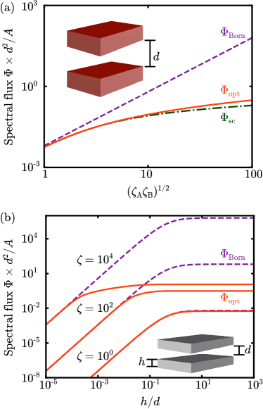
Figure 2: Comparison of $\Phi_{\mathrm{opt}}$ (solid orange) to $\Phi_{\mathrm{Born}}$ (dashed purple) and $\Phi_{\mathrm{sc}}$ (dot-dashed green) for two extended structures of infinite area $A$ and (a) infinite thickness or (b) finite thickness $h$ normalized to their mutual separation $d$. Both plots illustrate the behavior of $\Phi$ (normalized by $A/d^{2}$) with respect to material factors; $\Phi_{\mathrm{sc}}$ is not shown in (b) due to the near-overlap with $\Phi_{\mathrm{opt}}$.

Extended structures.— We now consider NFRHT between two extended structures of infinite area $A$ separated by a distance $d$. In this case, there is an infinite continuum of channels that may participate, labeled by the two-dimensional in-plane wavevector $\mathbf{k}$, and the sum over channels $i$ is written $\sum_{i}\to A\iint\frac{\mathrm{d}^{2}k}{(2\pi)^{2}}$. Furthermore, even after normalizing to the area, the Landauer bound $\Phi_{\mathrm{L}}/A=\iint\frac{1}{2\pi}\frac{d^{2}k}{(2\pi)^{2}}$ diverges, so we do not consider it further, and instead only consider $\Phi_{\mathrm{opt}}$, $\Phi_{\mathrm{Born}}$, and $\Phi_{\mathrm{sc}}$ after multiplying by a common factor of $\frac{d^{2}}{A}$, each of which only depend on the product of material factors $\sqrt{\zeta_{\mathrm{A}}\zeta_{\mathrm{B}}}$ and on no other length scales in the near-field.

As we show in the appendices, for two planar semi-infinite half-spaces constituting the bounding regions, these bounds take on particularly simple analytical forms, with

$$\Phi_{\mathrm{opt}}\times\frac{d^{2}}{A} =\frac{1}{4\pi^{2}}\ln\left(1+\frac{\zeta_{\mathrm{A}}\zeta_{\mathrm{B}}}{4}\right)\Theta(4-\zeta_{\mathrm{A}}\zeta_{\mathrm{B}})$$

$$+\frac{1}{8\pi^{2}}\left[\ln(\zeta_{\mathrm{A}}\zeta_{\mathrm{B}})+\ln^{2}\left(\frac{\zeta_{\mathrm{A}}\zeta_{\mathrm{B}}}{4}\right)^{1/2}\right]\Theta(\zeta_{\mathrm{A}}\zeta_{\mathrm{B}}-4),$$ (5)

while $\Phi_{\mathrm{sc}}\times\frac{d^{2}}{A}$ is given by the first term in (Fundamental limits to radiative heat transfer: the limited role of nanostructuring in the near-field) (without the Heaviside step function) and $\Phi_{\mathrm{Born}}\times\frac{d^{2}}{A}=\frac{\zeta_{\mathrm{A}}\zeta_{\mathrm{B}}}{16\pi^{2}}$. As observed in Fig. 2(a), all three bounds converge to one another for small $\zeta_{\mathrm{A}}\zeta_{\mathrm{B}}$, with $\Phi_{\mathrm{opt}}=\Phi_{\mathrm{sc}}$ for $\zeta_{\mathrm{A}}\zeta_{\mathrm{B}}\leq 4$. As $\zeta_{\mathrm{A}}\zeta_{\mathrm{B}}$ increases, the Born limits grossly overestimate the extent to which NFRHT can be optimized due to its simple linear dependence on $\zeta_{\mathrm{A}}\zeta_{\mathrm{B}}$, whereas the exact bound and scalar approximation grow with respect to $\zeta_{\mathrm{A}}\zeta_{\mathrm{B}}$ in a much slower logarithmic fashion. Strictly speaking, $\Phi_{\mathrm{opt}}$ grows faster than $\Phi_{\mathrm{sc}}$ as the latter grows as a logarithm while the former grows as the square of a logarithm, but in practice the difference is minute: $\sqrt{\zeta_{\mathrm{A}}\zeta_{\mathrm{B}}}$ would have to reach $10^{6}$ for the two quantities to differ even by a factor of 4. As a consequence, the bound can practically be reached by homogeneous isotropic planar bodies at the surface polariton resonance condition $\operatorname{Re}(1/\chi)=-1/2$, and the enhancement of $\Phi\times\frac{d^{2}}{A}$ relative to $\frac{1}{4\pi^{2}}$ will be $O(1)$ at best in practice regardless of the actual value of $\chi$ there. Thus, even more so than for dipolar bodies, there is very little room for improving $\Phi$ through nanostructuring compared to what can be achieved by planar polar-dielectric films.

We also evaluate $\Phi_{\mathrm{opt}}$ and $\Phi_{\mathrm{Born}}$ for planar films of finite thickness $h$ [Fig. 2(b)], and point out that each of these bounds only depends on $d$ and $h$ via the common term $\frac{A}{d^{2}}$ and via a function that depends only on $\zeta_{\mathrm{A}}\zeta_{\mathrm{B}}$ and the ratio $h/d$. In particular, we find that for thin films (compared to the separation), $\Phi_{\mathrm{opt}}$ converges to $\Phi_{\mathrm{Born}}$ for decreasing thickness at each value of $\zeta=\sqrt{\zeta_{\mathrm{A}}\zeta_{\mathrm{B}}}$, consistent with decreasing multiple scattering. However, as the thickness increases even to $h/d\approx 0.1$, each of these bounds quickly approaches its respective bulk asymptote in the limit $h/d\to\infty$. Moreover, the logarithmic scale on the plot makes clear that these asymptotic values of $\Phi_{\mathrm{Born}}$ grow linearly with $\zeta_{\mathrm{A}}\zeta_{\mathrm{B}}$, whereas the corresponding growth of $\Phi_{\mathrm{opt}}$ is logarithmic. We do not show $\Phi_{\mathrm{sc}}$ because it is so close to $\Phi_{\mathrm{opt}}$ in these regimes that the curves would be difficult to distinguish; this again suggests that while reaching the exact bounds for a given thickness $h$ would require nanoscale texturing, the bounds can be practically reached by planar films of the same thickness and appropriately chosen materials, in line with previous observations restricted to one-dimensionally periodic media Miller et al. (2014).

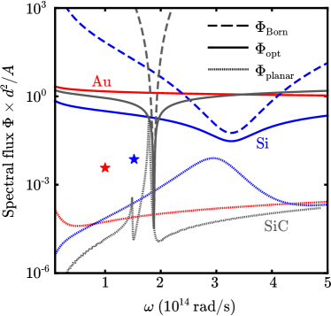
Figure 3: Comparison of $\Phi_{\mathrm{Born}}$ (dashed) and $\Phi_{\mathrm{opt}}$ (solid) for extended bodies to planar heat transfer $\Phi_{\mathrm{planar}}$ (dotted) at frequencies relevant to the Planck function at typical experimental temperatures, considering Au (red), doped Si (blue), and SiC (dark gray). Also shown are the maximum $\Phi$ of representative nanostructured Au (red star) Messina et al. (2017) and doped Si (blue star) Fernández-Hurtado et al. (2017) surfaces. $\Phi_{\mathrm{Born}}$ for Au is several orders of magnitude above the plotted range and thus not shown.

Finally, we compare the power spectrum $\Phi_{\mathrm{planar}}\times d^{2}/A$ associated with identical planar films Miller et al. (2015); Jin et al. (2017) to the exact and Born bounds in Fig. 3, specifically considering gold (Au), doped silicon (Si), and silicon carbide (SiC) as representative materials, as well as to the largest heat transfer observed in specific nanostructured Au Messina et al. (2017) and Si Fernández-Hurtado et al. (2017) surfaces studied in the past. (We employ Drude dispersions for Au Messina et al. (2017) and Si Fernández-Hurtado et al. (2017), and a phonon polaritonic dispersion for SiC Hong et al. (2018).) In particular, in the infrared where the Planck function is considerable (at typical experimental temperatures, $T\lesssim 1000\leavevmode\nobreak\ \mathrm{K}$), $\Phi_{\mathrm{Born}}$ for all of these materials is significantly larger than the corresponding $\Phi_{\mathrm{opt}}$ and is highly sensitive to material dispersion; as a specific example, the Born bound for Au lies significantly above the upper limits of the plot over the entire range of frequencies shown. By contrast, the logarithmic dependence of $\Phi_{\mathrm{opt}}$ on $\zeta_{p}$ means that it will generally be much less sensitive to changes in material dispersion except near polariton resonances; this is noticeable in the infrared for Si and more so for SiC, whereas Au does not feature material resonances except at much higher frequencies. We find that $\Phi_{\mathrm{planar}}$ is consistently much smaller than either $\Phi_{\mathrm{Born}}$ or $\Phi_{\mathrm{opt}}$ for Au owing to the lack of infrared resonances; the Au nanostructures of Messina et al. (2017) improve on the results for Au plates by two orders of magnitude, but still fall more than two orders of magnitude shy of $\Phi_{\mathrm{opt}}$ at that frequency. The outlook is more pessimistic for polar dielectrics like doped Si or SiC. Nanostructuring Si into a metasurface as in Fernández-Hurtado et al. (2017) barely improves $\Phi$ above the peak of the planar result, which never reaches its bound because the dispersion of Si prohibits the planar surface plasmon resonance condition $\operatorname{Re}(1/\chi)=-1/2$ from being reached; only the integrated NFRHT power $P$ increases substantially by virtue of the peak frequency being much smaller (i.e. escaping the exponential suppression of the Planck function). Meanwhile, SiC plates exhibit a power spectrum $\Phi$ that touches $\Phi_{\mathrm{opt}}$ at two points, the smaller of which is the material resonance where the losses become so large that the exact and Born limits coincide (as we have that shown multiple scattering becomes irrelevant for large dissipation), and the larger of which is a polaritonic resonance where $\Phi_{\mathrm{opt}}$ is nearly constant while $\Phi_{\mathrm{Born}}$ is larger by an unattainable factor of 50; we note that at those resonances, $\Phi_{\mathrm{planar}}=\Phi_{\mathrm{sc}}$.

Concluding remarks.— The results above suggest that apart from redshifting resonance frequencies to improve $P$ (especially useful for metals), nanostructuring of either dipolar or extended media cannot produce significantly better results for $\Phi$ than do spherical or planar objects, eventually saturating or exhibiting a logarithmic dependence on $\zeta=|\chi|^{2}/\operatorname{Im}(\chi)$ in each case. At first glance, this is a surprising contrast to the success of nanostructuring in enhancing the local density of states Miller et al. (2016). This dichotomy can be understood as a consequence of finite-size effects: a dipole radiator does not scatter fields and hence an infinite number of modes can participate in absorption, but this cannot hold for objects of finite size.

While we have focused on NFRHT at individual resonance frequencies, their narrow bandwidths $\Delta\omega\sim\omega\frac{\operatorname{Im}(\chi)}{|\chi|}$ permit approximate bounds on the integrated heat transfer Miller et al. (2015). For two bodies of the same susceptibility $\chi$, this yields:

$$P_{\mathrm{opt}}\approx\frac{\omega\operatorname{Im}(\chi)}{|\chi|}\Phi_{\mathrm{opt}}(\omega)[\Pi(\omega,T_{\mathrm{B}})-\Pi(\omega,T_{\mathrm{A}})].$$

For dipolar bodies, $\Phi_{\mathrm{opt}}$ reaches a maximum with respect to $\zeta$ and never diverges, while for extended structures the divergence is logarithmic. Hence, beyond a threshold, any increase in $\Phi_{\mathrm{opt}}$ from larger material response will be accompanied by a corresponding decrease in $\Delta\omega$; this suggests that regardless of object sizes, there exists an optimal $\zeta$ maximizing $P$.

Finally, we emphasize that the above analyses focused on the near-field, which can be justified for small enough separations, but $\Phi_{\mathrm{opt}}$ and $\Phi_{\mathrm{sc}}$ in general can be evaluated at every lengthscale, whereas the same cannot be said of $\Phi_{\mathrm{Born}}$. That said, as discussed in Molesky et al. (2019), our bounds do not explicitly include the effects of far-field radiative losses, which in conjunction with multiple scattering should provide even tighter bounds. Additionally, similar bounds could be derived for other problems in fluctuational electromagnetism, including fluorescence energy transfer Polimeridis et al. (2015) and Casimir forces Kenneth and Klich (2006), the subject of future work.

Acknowledgments.—The authors would like to thank Riccardo Messina and Pengning Chao for helpful discussions. This work was supported by the National Science Foundation under Grants No. DMR-1454836, DMR 1420541, DGE 1148900, the Cornell Center for Materials Research MRSEC (award no. DMR-1719875), and the Defense Advanced Research Projects Agency (DARPA) under agreement HR00111820046. The views, opinions and/or findings expressed are those of the authors and should not be interpreted as representing the official views or policies of the Department of Defense or the U.S. Government.

Appendix A Notation

We briefly discuss the notation used through the main text and the appendices. A vector field $\mathbf{v}(\mathbf{x})$ will be denoted as $|\mathbf{v}\rangle$. The conjugated inner product is $\langle\mathbf{u},\mathbf{v}\rangle=\int\leavevmode\nobreak\ \mathrm{d}^{3}x\leavevmode\nobreak\ \mathbf{u}^{\star}(\mathbf{x})\cdot\mathbf{v}(\mathbf{x})$. An operator $\mathbb{A}(\mathbf{x},\mathbf{x}^{\prime})$ will be denoted as $\mathbb{A}$, with $\int\leavevmode\nobreak\ \mathrm{d}^{3}x^{\prime}\leavevmode\nobreak\ \mathbb{A}(\mathbf{x},\mathbf{x}^{\prime})\cdot\mathbf{v}(\mathbf{x}^{\prime})$ denoted as $\mathbb{A}|\mathbf{v}\rangle$. The Hermitian conjugate $\mathbb{A}^{\dagger}$ is defined such that $\langle\mathbf{u},\mathbb{A}^{\dagger}\mathbf{v}\rangle=\langle\mathbb{A}\mathbf{u},\mathbf{v}\rangle$. The anti-Hermitian part of a square operator (whose domain and range are the same size) is defined as the operator $\operatorname{asym}(\mathbb{A})=(\mathbb{A}-\mathbb{A}^{\dagger})/(2i)$. Finally, the trace of an operator is $\operatorname{Tr}(\mathbb{A})=\int\leavevmode\nobreak\ \mathrm{d}^{3}x\leavevmode\nobreak\ \operatorname{Tr}(\mathbb{A}(\mathbf{x},\mathbf{x}))$. Through this paper, unless stated explicitly otherwise, all quantities implicitly depend on $\omega$, and such dependence will be notationally suppressed for brevity.

Appendix B Properties of $\Phi_{\mathrm{sc}}$

In this section, we show that the scalar approximation to the bound on NFRHT between two bodies A and B in vacuum exhibits a local stationary point when both bodies satisfy the optimal absorption condition in isolation. We also show that the scalar approximation in the near-field is domain monotonic, meaning that it can be evaluated for larger domains than the bodies in question given their material response factors. These results make use of the fact that in the absence of retardation, $\mathbb{G}^{\mathrm{vac}}_{\mathrm{BA}}=(\mathbb{G}^{\mathrm{vac}}_{\mathrm{AB}})^{\top}$ is a real-valued operator in position-space, so $\mathbb{G}^{\mathrm{vac}}_{\mathrm{BA}}\mathbb{G}^{\mathrm{vac}}_{\mathrm{AB}}$ is a Hermitian positive-semidefinite operator.

B.1 Stationarity of the scalar approximation

In this section, we prove that $\Phi_{\mathrm{sc}}$ in the near-field exhibits a local stationary point when the T-operators Molesky et al. (2019) of each body satisfy the condition of zero far-field scattering in isolation. Thus, if body A is fixed to be an isolated perfect absorber satisfying $\mathbb{T}_{\mathrm{A}}=i\zeta_{\mathrm{A}}\mathbb{I}_{\mathrm{A}}$, then any change to body B from perfect absorption, written as $\mathbb{T}_{\mathrm{B}}=\zeta_{\mathrm{B}}\left(i\mathbb{I}_{\mathrm{B}}+\zeta_{\mathrm{B}}^{-1}\mathbb{R}\right)$ for a small perturbation $\mathbb{R}$ (restricted to be real symmetric to preserve the condition of zero far-field scattering by $\mathbb{T}_{\mathrm{B}}$), produces no change in the NFRHT to first order. By reciprocity, the same arguments hold if A and B are exchanged.

Defining the real symmetric positive-semidefinite operator $\mathbb{K}=\zeta_{\mathrm{A}}\zeta_{\mathrm{B}}\mathbb{G}^{\mathrm{vac}}_{\mathrm{BA}}\mathbb{G}^{\mathrm{vac}}_{\mathrm{AB}}$ and replacing $\mathbb{I}_{\mathrm{B}}$ by $\mathbb{I}$ for notational convenience, NFRHT may be written as

$$\Phi=\frac{2}{\pi}\operatorname{Tr}\Bigg{[}\left(\mathbb{I}+\mathbb{K}+i\mathbb{K}\mathbb{R}\right)^{-1}\times\\ \left(\mathbb{I}_{\mathrm{B}}-(-i\mathbb{I}+\mathbb{R})\frac{\operatorname{Im}(\mathbb{G}^{\mathrm{vac}})}{\lambda_{\mathrm{B}}}(i\mathbb{I}+\mathbb{R})\right)\times\\ \left(\mathbb{I}+\mathbb{K}-i\mathbb{K}\mathbb{R}\right)^{-1}\mathbb{K}\Bigg{]}$$ (6)

where we have used the facts that $\mathbb{T}_{\mathrm{A}}\operatorname{Im}(\mathbb{V}_{\mathrm{A}}^{-1\star})\mathbb{T}_{\mathrm{A}}^{\star}=\zeta_{\mathrm{A}}\mathbb{I}_{\mathrm{A}}$ and that in general, $\mathbb{T}_{\mathrm{B}}^{\star}\operatorname{Im}(\mathbb{V}_{\mathrm{B}}^{-1\star})\mathbb{T}_{\mathrm{B}}=\operatorname{Im}(\mathbb{T}_{\mathrm{B}})-\mathbb{T}_{\mathrm{B}}^{\star}\operatorname{Im}(\mathbb{G}^{\mathrm{vac}})\mathbb{T}_{\mathrm{B}}$, after which point the definition of $\mathbb{T}_{\mathrm{B}}$ in terms of $\mathbb{R}$ may be substituted. This trace can be expanded order-by-order in $\mathbb{R}$, with $\Phi^{(n)}$ denoting the $n$th order term.

The lowest-order term is given by,

$$\Phi_{\mathrm{sc}}^{(0)}=\frac{2}{\pi}\operatorname{Tr}\Bigg{[}\left(\mathbb{I}+\mathbb{K}\right)^{-1}\left(\mathbb{I}_{\mathrm{B}}-\frac{\operatorname{Im}(\mathbb{G}^{\mathrm{vac}})}{\lambda_{\mathrm{B}}}\right)\left(\mathbb{I}+\mathbb{K}\right)^{-1}\mathbb{K}\Bigg{]}$$ (7)

which, upon undoing the substitution $\mathbb{T}_{\mathrm{B}}^{\star}\operatorname{Im}(\mathbb{V}_{\mathrm{B}}^{-1\star})\mathbb{T}_{\mathrm{B}}=\operatorname{Im}(\mathbb{T}_{\mathrm{B}})-\mathbb{T}_{\mathrm{B}}^{\star}\operatorname{Im}(\mathbb{G}^{\mathrm{vac}})\mathbb{T}_{\mathrm{B}}$ and the definition of $\mathbb{T}_{\mathrm{B}}$ in terms of $\mathbb{R}$, is identical to the result in the main text.

The first-order term is given by,

$$\Phi_{\mathrm{sc}}^{(1)}=\frac{2}{\pi}\operatorname{Tr}\Bigg{[}-\frac{i}{\lambda_{\mathrm{B}}}(\mathbb{I}+\mathbb{K})^{-1}\mathbb{R}\operatorname{Im}(\mathbb{G}^{\mathrm{vac}})(\mathbb{I}+\mathbb{K})^{-1}\mathbb{K}+\\ \frac{i}{\lambda_{\mathrm{B}}}(\mathbb{I}+\mathbb{K})^{-1}\operatorname{Im}(\mathbb{G}^{\mathrm{vac}})\mathbb{R}(\mathbb{I}+\mathbb{K})^{-1}\mathbb{K}-\\ i(\mathbb{I}+\mathbb{K})^{-1}\mathbb{R}\mathbb{K}(\mathbb{I}+\mathbb{K})^{-1}\left(\mathbb{I}-\frac{\operatorname{Im}(\mathbb{G}^{\mathrm{vac}})}{\lambda_{\mathrm{B}}}\right)(\mathbb{I}+\mathbb{K})^{-1}\mathbb{K}+\\ i(\mathbb{I}+\mathbb{K})^{-1}\left(\mathbb{I}-\frac{\operatorname{Im}(\mathbb{G}^{\mathrm{vac}})}{\lambda_{\mathrm{B}}}\right)(\mathbb{I}+\mathbb{K})^{-1}\mathbb{K}\mathbb{R}(\mathbb{I}+\mathbb{K})^{-1}\mathbb{K}\Bigg{]}$$ (8)

but by exploiting the invariance of the trace under cyclic permutation and transposition, and noting that $\mathbb{K}=\mathbb{K}^{\top}$ and $\mathbb{R}=\mathbb{R}^{\top}$, this trace actually vanishes. Therefore, each body satisfying perfect absorption in isolation produces a local stationary point in $\Phi_{\mathrm{sc}}$.

B.2 Domain monotonicity of $\Phi_{\mathrm{sc}}$

We now prove that the $\Phi_{\mathrm{sc}}$ factor is domain monotonic, meaning that it will always increase when the spatial domain (i.e. the volume of either body) increases; this has previously been proven for the scalar Laplace operator with Dirichlet boundaries Grebenkov and Nguyen (2013) but to our knowledge, not for $\frac{2}{\pi}\zeta_{\mathrm{A}}\zeta_{\mathrm{B}}\left\lVert(\mathbb{I}_{\mathrm{B}}+\zeta_{\mathrm{A}}\zeta_{\mathrm{B}}\mathbb{G}^{\mathrm{vac}}_{\mathrm{BA}}\mathbb{G}^{\mathrm{vac}}_{\mathrm{AB}})^{-1}\mathbb{G}^{\mathrm{vac}}_{\mathrm{BA}}\right\rVert_{\mathrm{F}}^{2}$. We allow bodies A and B to have different shapes, sizes, and material response factors $\zeta_{p}$ for $p\in\{\mathrm{A},\mathrm{B}\}$, and we assume only that $\zeta_{p}$ as well as the minimum separation $d$ are fixed throughout this proof. In particular, we assume a small enough perturbative increase to the volume of either object so that each object remains an optimal absorber even with the new volume, i.e. $\mathbb{T}_{p}=i\zeta_{p}\mathbb{I}_{p}$ is still true even with the new degrees of freedom. If body B undergoes a perturbative increase in volume while body A remains unchanged, the projection operator onto the original volume of B (comprising the actual material degrees of freedom, not the entire convex hull, which is relevant if the original volume of B has interior holes or surface concavities) will be denoted as $\mathbb{P}_{0}$, while the projection operator onto the added material volume in B will be denoted as $\mathbb{P}_{\Delta}$, with $\mathbb{P}_{0}\mathbb{P}_{\Delta}=\mathbb{P}_{\Delta}\mathbb{P}_{0}=0$ encoding the disjointness of the two spaces. Denoting $\mathbb{G}^{\mathrm{vac}}_{\mathrm{B}_{0}\mathrm{A}}=\mathbb{P}_{0}\mathbb{G}^{\mathrm{vac}}_{\mathrm{BA}}$, $\mathbb{G}^{\mathrm{vac}}_{\Delta\mathrm{BA}}=\mathbb{P}_{\Delta}\mathbb{G}^{\mathrm{vac}}_{\mathrm{BA}}$, $\mathbb{G}^{\mathrm{vac}}_{\mathrm{AB}_{0}}=(\mathbb{G}^{\mathrm{vac}}_{\mathrm{B}_{0}\mathrm{A}})^{\top}$, and $\mathbb{G}^{\mathrm{vac}}_{\mathrm{A}\Delta\mathrm{B}}=(\mathbb{G}^{\mathrm{vac}}_{\Delta\mathrm{BA}})^{\top}$, and defining

$$\begin{split}\mathbb{G}^{\mathrm{vac}}_{\mathrm{BA}}&=\begin{bmatrix}\mathbb{G}^{\mathrm{vac}}_{\mathrm{B}_{0}\mathrm{A}}\\ \mathbb{G}^{\mathrm{vac}}_{\Delta\mathrm{BA}}\end{bmatrix}\\ \mathbb{G}^{\mathrm{vac}}_{\mathrm{AB}}&=\begin{bmatrix}\mathbb{G}^{\mathrm{vac}}_{\mathrm{AB}_{0}}&\mathbb{G}^{\mathrm{vac}}_{\mathrm{A}\Delta\mathrm{B}}\end{bmatrix}\\ \mathbb{I}_{\mathrm{B}}&=\begin{bmatrix}\mathbb{P}_{0}&0\\ 0&\mathbb{P}_{\Delta}\end{bmatrix}\end{split}$$ (9)

allows for writing (in a slight abuse of notation)

$$\begin{split}\mathbb{G}^{\mathrm{vac}}_{\mathrm{BA}}\mathbb{G}^{\mathrm{vac}}_{\mathrm{AB}}&\equiv\mathbb{G}^{\mathrm{vac}}_{\mathrm{B}_{0}\mathrm{A}}\mathbb{G}^{\mathrm{vac}}_{\mathrm{AB}_{0}}+\Delta(\mathbb{G}^{\mathrm{vac}}_{\mathrm{BA}}\mathbb{G}^{\mathrm{vac}}_{\mathrm{AB}})\\ \mathbb{G}^{\mathrm{vac}}_{\mathrm{B}_{0}\mathrm{A}}\mathbb{G}^{\mathrm{vac}}_{\mathrm{AB}_{0}}&\equiv\begin{bmatrix}\mathbb{G}^{\mathrm{vac}}_{\mathrm{B}_{0}\mathrm{A}}\mathbb{G}^{\mathrm{vac}}_{\mathrm{AB}_{0}}&0\\ 0&0\end{bmatrix}\\ \Delta(\mathbb{G}^{\mathrm{vac}}_{\mathrm{BA}}\mathbb{G}^{\mathrm{vac}}_{\mathrm{AB}})&\equiv\begin{bmatrix}0&\mathbb{G}^{\mathrm{vac}}_{\mathrm{B}_{0}\mathrm{A}}\mathbb{G}^{\mathrm{vac}}_{\mathrm{A}\Delta\mathrm{B}}\\ \mathbb{G}^{\mathrm{vac}}_{\Delta\mathrm{BA}}\mathbb{G}^{\mathrm{vac}}_{\mathrm{AB}_{0}}&\mathbb{G}^{\mathrm{vac}}_{\Delta\mathrm{BA}}\mathbb{G}^{\mathrm{vac}}_{\mathrm{A}\Delta\mathrm{B}}\end{bmatrix}\end{split}$$ (10)

for this system. This in turn leads to the expression,

$$(\mathbb{I}_{\mathrm{B}}+\zeta_{\mathrm{A}}\zeta_{\mathrm{B}}\mathbb{G}^{\mathrm{vac}}_{\mathrm{BA}}\mathbb{G}^{\mathrm{vac}}_{\mathrm{AB}})^{-1}\\ =(\mathbb{I}_{\mathrm{B}}+\zeta_{\mathrm{A}}\zeta_{\mathrm{B}}\mathbb{G}^{\mathrm{vac}}_{\mathrm{B}_{0}\mathrm{A}}\mathbb{G}^{\mathrm{vac}}_{\mathrm{AB}_{0}})^{-1}\\ -\zeta_{\mathrm{A}}\zeta_{\mathrm{B}}(\mathbb{I}_{\mathrm{B}}+\zeta_{\mathrm{A}}\zeta_{\mathrm{B}}\mathbb{G}^{\mathrm{vac}}_{\mathrm{B}_{0}\mathrm{A}}\mathbb{G}^{\mathrm{vac}}_{\mathrm{AB}_{0}})^{-1}\\ \times\Delta(\mathbb{G}^{\mathrm{vac}}_{\mathrm{BA}}\mathbb{G}^{\mathrm{vac}}_{\mathrm{AB}})(\mathbb{I}_{\mathrm{B}}+\zeta_{\mathrm{A}}\zeta_{\mathrm{B}}\mathbb{G}^{\mathrm{vac}}_{\mathrm{B}_{0}\mathrm{A}}\mathbb{G}^{\mathrm{vac}}_{\mathrm{AB}_{0}})^{-1}\\ +O((\Delta(\mathbb{G}^{\mathrm{vac}}_{\mathrm{BA}}\mathbb{G}^{\mathrm{vac}}_{\mathrm{AB}}))^{2}),$$ (11)

to lowest order in the term $\Delta(\mathbb{G}^{\mathrm{vac}}_{\mathrm{BA}}\mathbb{G}^{\mathrm{vac}}_{\mathrm{AB}})$, which is small as the addition to the volume of B is small (perturbative). Plugging this into the expression for $\Phi_{\mathrm{sc}}$ and exploiting the cyclic property of the trace for notational convenience yields,

$$\operatorname{Tr}(\mathbb{G}^{\mathrm{vac}}_{\mathrm{BA}}\mathbb{G}^{\mathrm{vac}}_{\mathrm{AB}}(\mathbb{I}_{\mathrm{B}}+\zeta_{\mathrm{A}}\zeta_{\mathrm{B}}\mathbb{G}^{\mathrm{vac}}_{\mathrm{BA}}\mathbb{G}^{\mathrm{vac}}_{\mathrm{AB}})^{-2})=\\ \operatorname{Tr}(\mathbb{G}^{\mathrm{vac}}_{\mathrm{B}_{0}\mathrm{A}}\mathbb{G}^{\mathrm{vac}}_{\mathrm{AB}_{0}}(\mathbb{I}_{\mathrm{B}}+\zeta_{\mathrm{A}}\zeta_{\mathrm{B}}\mathbb{G}^{\mathrm{vac}}_{\mathrm{B}_{0}\mathrm{A}}\mathbb{G}^{\mathrm{vac}}_{\mathrm{AB}_{0}})^{-2})\\ +\operatorname{Tr}(\Delta(\mathbb{G}^{\mathrm{vac}}_{\mathrm{BA}}\mathbb{G}^{\mathrm{vac}}_{\mathrm{AB}})(\mathbb{I}_{\mathrm{B}}+\zeta_{\mathrm{A}}\zeta_{\mathrm{B}}\mathbb{G}^{\mathrm{vac}}_{\mathrm{B}_{0}\mathrm{A}}\mathbb{G}^{\mathrm{vac}}_{\mathrm{AB}_{0}})^{-2})\\ -2\zeta_{\mathrm{A}}\zeta_{\mathrm{B}}\operatorname{Tr}(\Delta(\mathbb{G}^{\mathrm{vac}}_{\mathrm{BA}}\mathbb{G}^{\mathrm{vac}}_{\mathrm{AB}})(\mathbb{I}_{\mathrm{B}}+\zeta_{\mathrm{A}}\zeta_{\mathrm{B}}\mathbb{G}^{\mathrm{vac}}_{\mathrm{B}_{0}\mathrm{A}}\mathbb{G}^{\mathrm{vac}}_{\mathrm{AB}_{0}})^{-3}\\ \times\mathbb{G}^{\mathrm{vac}}_{\mathrm{B}_{0}\mathrm{A}}\mathbb{G}^{\mathrm{vac}}_{\mathrm{AB}_{0}})+O((\Delta(\mathbb{G}^{\mathrm{vac}}_{\mathrm{BA}}\mathbb{G}^{\mathrm{vac}}_{\mathrm{AB}}))^{2})$$ (12)

to lowest order in the term $\Delta(\mathbb{G}^{\mathrm{vac}}_{\mathrm{BA}}\mathbb{G}^{\mathrm{vac}}_{\mathrm{AB}})$, for which each of the three terms may be analyzed individually. The first term is merely the unperturbed contribution to $\Phi_{\mathrm{sc}}$, so the perturbation to lowest order comprises the second and third terms. For the second term, the factor

$$(\mathbb{I}_{\mathrm{B}}+\zeta_{\mathrm{A}}\zeta_{\mathrm{B}}\mathbb{G}^{\mathrm{vac}}_{\mathrm{B}_{0}\mathrm{A}}\mathbb{G}^{\mathrm{vac}}_{\mathrm{AB}_{0}})^{-2}\\ =\begin{bmatrix}(\mathbb{P}_{0}+\zeta_{\mathrm{A}}\zeta_{\mathrm{B}}\mathbb{G}^{\mathrm{vac}}_{\mathrm{B}_{0}\mathrm{A}}\mathbb{G}^{\mathrm{vac}}_{\mathrm{AB}_{0}})^{-2}&0\\ 0&\mathbb{P}_{\Delta}\end{bmatrix}$$

leads to

$$\Delta(\mathbb{G}^{\mathrm{vac}}_{\mathrm{BA}}\mathbb{G}^{\mathrm{vac}}_{\mathrm{AB}})(\mathbb{I}_{\mathrm{B}}+\zeta_{\mathrm{A}}\zeta_{\mathrm{B}}\mathbb{G}^{\mathrm{vac}}_{\mathrm{B}_{0}\mathrm{A}}\mathbb{G}^{\mathrm{vac}}_{\mathrm{AB}_{0}})^{-2}\\ =\begin{bmatrix}0&\mathbb{G}^{\mathrm{vac}}_{\mathrm{B}_{0}\mathrm{A}}\mathbb{G}^{\mathrm{vac}}_{\mathrm{A}\Delta\mathrm{B}}\\ \mathbb{G}^{\mathrm{vac}}_{\Delta\mathrm{BA}}\mathbb{G}^{\mathrm{vac}}_{\mathrm{AB}_{0}}(\mathbb{P}_{0}+\zeta_{\mathrm{A}}\zeta_{\mathrm{B}}\mathbb{G}^{\mathrm{vac}}_{\mathrm{B}_{0}\mathrm{A}}\mathbb{G}^{\mathrm{vac}}_{\mathrm{AB}_{0}})^{-2}&\mathbb{G}^{\mathrm{vac}}_{\Delta\mathrm{BA}}\mathbb{G}^{\mathrm{vac}}_{\mathrm{A}\Delta\mathrm{B}}\end{bmatrix}$$

whose trace is simply $\operatorname{Tr}(\mathbb{G}^{\mathrm{vac}}_{\Delta\mathrm{BA}}\mathbb{G}^{\mathrm{vac}}_{\mathrm{A}\Delta\mathrm{B}})$. For the third term, the factor

$$(\mathbb{I}_{\mathrm{B}}+\zeta_{\mathrm{A}}\zeta_{\mathrm{B}}\mathbb{G}^{\mathrm{vac}}_{\mathrm{B}_{0}\mathrm{A}}\mathbb{G}^{\mathrm{vac}}_{\mathrm{AB}_{0}})^{-3}\mathbb{G}^{\mathrm{vac}}_{\mathrm{B}_{0}\mathrm{A}}\mathbb{G}^{\mathrm{vac}}_{\mathrm{AB}_{0}}\\ =\begin{bmatrix}(\mathbb{P}_{0}+\zeta_{\mathrm{A}}\zeta_{\mathrm{B}}\mathbb{G}^{\mathrm{vac}}_{\mathrm{B}_{0}\mathrm{A}}\mathbb{G}^{\mathrm{vac}}_{\mathrm{AB}_{0}})^{-3}\mathbb{G}^{\mathrm{vac}}_{\mathrm{B}_{0}\mathrm{A}}\mathbb{G}^{\mathrm{vac}}_{\mathrm{AB}_{0}}&0\\ 0&0\end{bmatrix}$$

leads to

$$\begin{split}&\Delta(\mathbb{G}^{\mathrm{vac}}_{\mathrm{BA}}\mathbb{G}^{\mathrm{vac}}_{\mathrm{AB}})(\mathbb{I}_{\mathrm{B}}+\zeta_{\mathrm{A}}\zeta_{\mathrm{B}}\mathbb{G}^{\mathrm{vac}}_{\mathrm{B}_{0}\mathrm{A}}\mathbb{G}^{\mathrm{vac}}_{\mathrm{AB}_{0}})^{-3}\mathbb{G}^{\mathrm{vac}}_{\mathrm{B}_{0}\mathrm{A}}\mathbb{G}^{\mathrm{vac}}_{\mathrm{AB}_{0}}=\\ &\begin{bmatrix}0&0\\ \mathbb{G}^{\mathrm{vac}}_{\Delta\mathrm{BA}}\mathbb{G}^{\mathrm{vac}}_{\mathrm{AB}_{0}}(\mathbb{P}_{0}+\zeta_{\mathrm{A}}\zeta_{\mathrm{B}}\mathbb{G}^{\mathrm{vac}}_{\mathrm{B}_{0}\mathrm{A}}\mathbb{G}^{\mathrm{vac}}_{\mathrm{AB}_{0}})^{-3}\mathbb{G}^{\mathrm{vac}}_{\mathrm{B}_{0}\mathrm{A}}\mathbb{G}^{\mathrm{vac}}_{\mathrm{AB}_{0}}&0\end{bmatrix}\end{split}$$

whose trace vanishes. Therefore, a perturbative increase in the volume of body B changes the contribution to $\Phi_{\mathrm{sc}}$ by an amount $\operatorname{Tr}(\mathbb{G}^{\mathrm{vac}}_{\Delta\mathrm{BA}}\mathbb{G}^{\mathrm{vac}}_{\mathrm{A}\Delta\mathrm{B}})$, independent of $\zeta_{p}$ for $p\in\{\mathrm{A},\mathrm{B}\}$; as $\mathbb{G}^{\mathrm{vac}}_{\Delta\mathrm{BA}}=(\mathbb{G}^{\mathrm{vac}}_{\mathrm{A}\Delta\mathrm{B}})^{\top}$ is real-valued in the near-field, then $\mathbb{G}^{\mathrm{vac}}_{\Delta\mathrm{BA}}\mathbb{G}^{\mathrm{vac}}_{\mathrm{A}\Delta\mathrm{B}}$ is real-symmetric positive-semidefinite, so its trace is nonnegative, and is exactly the pairwise additive contribution to $\left\lVert\mathbb{G}^{\mathrm{vac}}_{\mathrm{BA}}\right\rVert_{\mathrm{F}}^{2}$ (in the absence of multiple scattering) from the same perturbation. Reciprocity implies invariance of this contribution to $\Phi_{\mathrm{sc}}$ under interchange of bodies A and B, which means that the same arguments can be used to show that a perturbative increase in the volume of A (holding B fixed) increases the contribution to $\Phi_{\mathrm{sc}}$. As both of these statements are true regardless of the original geometries of A and B, they must remain true for any combination of increases in the volumes of A and B, even if the minimum separation $d$ does not change. As a result, for a given $d$ and $\zeta_{p}$ for $p\in\{\mathrm{A},\mathrm{B}\}$, the volume that maximizes the domain of the scattering operators (a planar semi-infinite half-space and its geometric mirror image, though $\zeta_{\mathrm{A}}$ and $\zeta_{\mathrm{B}}$ may differ), leads to their largest $\Phi_{\mathrm{sc}}$. For such restricted T-operators, nanostructuring will therefore always decrease $\Phi_{\mathrm{sc}}$ for fixed $d$ and material response factors.

Appendix C Singular values of $\mathbb{G}^{\mathrm{vac}}_{\mathrm{BA}}$ for dipolar particles

In this section, we derive analytical expressions for the singular values $g_{i}$ of $\mathbb{G}^{\mathrm{vac}}_{\mathrm{BA}}$ in the near-field, where body B is a dipolar nanoparticle and body A is either another dipolar nanoparticle or an extended object. We start with the case of two dipoles. This means for each body $p\in\{\mathrm{A},\mathrm{B}\}$, the relevant basis functions are $\mathbf{a}_{i}(\mathbf{x})=\sqrt{V_{\mathrm{A}}}\delta^{3}(\mathbf{x}-\mathbf{r}_{\mathrm{A}})\mathbf{e}_{i}$ and $\mathbf{b}_{i}(\mathbf{x})=\sqrt{V_{\mathrm{B}}}\delta^{3}(\mathbf{x}-\mathbf{r}_{\mathrm{B}})\mathbf{e}_{i}$. Without loss of generality, we take $\mathbf{r}_{\mathrm{A}}=0$ and $\mathbf{r}_{\mathrm{B}}=d\mathbf{e}_{z}$. This means that we write the near-field Green’s function tensor in position space as $\langle\mathbf{b}_{i},\mathbb{G}^{\mathrm{vac}}_{\mathrm{BA}}\mathbf{a}_{j}\rangle=\frac{\sqrt{V_{\mathrm{A}}V_{\mathrm{B}}}}{4\pi d^{3}}\left(3\delta_{i,3}\delta_{j,3}-\delta_{ij}\right)$. As a result, we may immediately read off the singular values $g_{1}=g_{2}=\frac{\sqrt{V_{\mathrm{A}}V_{\mathrm{B}}}}{4\pi d^{3}}$ and $g_{3}=2g_{1}=\frac{\sqrt{V_{\mathrm{A}}V_{\mathrm{B}}}}{2\pi d^{3}}$.

We now consider a situation in which body B remains dipolar but body A is replaced by an extended object enclosed by the semi-infinite half-space $z\leq 0$; for simplicity, we will denote $V_{\mathrm{B}}$ simply as $V$. Without loss of generality, we still take $\mathbf{r}_{\mathrm{B}}=d\mathbf{e}_{z}$ and $\mathbf{b}_{i}(\mathbf{x})=\sqrt{V_{\mathrm{B}}}\delta^{3}(\mathbf{x}-\mathbf{r}_{\mathrm{B}})\mathbf{e}_{i}$. Normalizable basis functions for body A are harder to define due to the semi-infinite domain. However, because the singular values of $\mathbb{G}^{\mathrm{vac}}_{\mathrm{BA}}$ are simply the eigenvalues of $\mathbb{G}^{\mathrm{vac}}_{\mathrm{BA}}\mathbb{G}_{\mathrm{AB}}^{\mathrm{vac}\star}$, and because $\mathbb{G}^{\mathrm{vac}}_{\mathrm{BA}}$ is real-valued in the near-field, we need only to evaluate the matrix elements $\langle\mathbf{b}_{i},\mathbb{G}^{\mathrm{vac}}_{\mathrm{BA}}\mathbb{G}^{\mathrm{vac}}_{\mathrm{AB}}\mathbf{b}_{j}\rangle$, where the operator product $\mathbb{G}^{\mathrm{vac}}_{\mathrm{BA}}\mathbb{G}^{\mathrm{vac}}_{\mathrm{AB}}$ can be evaluated in position space. This evaluation yields

$$\sum_{k}\int_{V_{\mathrm{A}}}G^{\mathrm{vac}}_{ik}(\mathbf{r}_{\mathrm{B}},\mathbf{x})\cdot G^{\mathrm{vac}}_{kj}(\mathbf{x},\mathbf{r}_{\mathrm{B}})\leavevmode\nobreak\ \mathrm{d}^{3}\mathbf{x}=\\ V\int_{-\infty}^{\infty}\int_{-\infty}^{\infty}\int_{-\infty}^{0}\frac{\mathrm{d}x\leavevmode\nobreak\ \mathrm{d}y\leavevmode\nobreak\ \mathrm{d}z}{16\pi^{2}|\mathbf{r}_{\mathrm{B}}-\mathbf{x}|^{6}}\left(\frac{3(d\delta_{i,3}-x_{i})(d\delta_{j,3}-x_{j})}{|\mathbf{r}_{\mathrm{B}}-\mathbf{x}|^{2}}+\delta_{ij}\right)$$

and this integral can be evaluated in cylindrical coordinates with $\mathbf{x}=\rho(\cos(\varphi)\mathbf{e}_{x}+\sin(\varphi)\mathbf{e}_{y})+z\mathbf{e}_{z}$, so $|\mathbf{r}_{\mathrm{B}}-\mathbf{x}|^{2}=\rho^{2}+(d-z)^{2}$. The term involving $\delta_{ij}$ can easily be evaluated due to independence from $\varphi$, yielding:

$$\frac{V\delta_{ij}}{8\pi}\int_{0}^{\infty}\int_{-\infty}^{0}\frac{1}{(\rho^{2}+(d-z)^{2})^{3}}\rho\leavevmode\nobreak\ \mathrm{d}z\leavevmode\nobreak\ \mathrm{d}\rho=\frac{V\delta_{ij}}{96\pi d^{3}}$$

by integrating over $\rho$ and then $z$. The term involving $(d\delta_{i,3}-x_{i})(d\delta_{j,3}-x_{j})$ requires evaluation of this outer product of vectors. In cylindrical coordinates, this evaluates as the tensor

$$(\mathbf{r}_{\mathrm{B}}-\mathbf{x})\otimes(\mathbf{r}_{\mathrm{B}}-\mathbf{x})=\\ \begin{bmatrix}\rho^{2}\cos^{2}(\varphi)&\rho^{2}\cos(\varphi)\sin(\varphi)&\rho\cos(\varphi)(d-z)\\ \rho^{2}\cos(\varphi)\sin(\varphi)&\rho^{2}\sin^{2}(\varphi)&\rho\sin(\varphi)(d-z)\\ \rho\cos(\varphi)(d-z)&\rho\sin(\varphi)(d-z)&(d-z)^{2}\end{bmatrix}$$

for which integration over $\varphi$ makes the off-diagonal elements vanish, while integration over the diagonal elements gives $\rho^{2}\int_{0}^{2\pi}\cos^{2}(\varphi)\leavevmode\nobreak\ \mathrm{d}\varphi=\rho^{2}\int_{0}^{2\pi}\sin^{2}(\varphi)\leavevmode\nobreak\ \mathrm{d}\varphi=\pi\rho^{2}$ for the $xx$- and $yy$-components or $(d-z)^{2}\int_{0}^{2\pi}\mathrm{d}\varphi=2\pi(d-z)^{2}$ for the $zz$-component. The integral over the $xx$- and $yy$-components therefore yield:

$$\frac{3V}{16\pi}\int_{0}^{\infty}\int_{-\infty}^{0}\frac{\rho^{3}\leavevmode\nobreak\ \mathrm{d}z\leavevmode\nobreak\ \mathrm{d}\rho}{(\rho^{2}+(d-z)^{2})^{4}}=\frac{V}{192\pi d^{3}}$$

while the integral over the $zz$-component yields

$$\frac{3V}{8\pi}\int_{0}^{\infty}\int_{-\infty}^{0}\frac{\rho(d-z)^{2}\leavevmode\nobreak\ \mathrm{d}z\leavevmode\nobreak\ \mathrm{d}\rho}{(\rho^{2}+(d-z)^{2})^{4}}=\frac{V}{48\pi d^{3}}.$$

Adding these contributions to the contributions from the prefactor of $\delta_{ij}$ yields:

$$\langle\mathbf{b}_{i},\mathbb{G}^{\mathrm{vac}}_{\mathrm{BA}}\mathbb{G}^{\mathrm{vac}}_{\mathrm{AB}}\mathbf{b}_{j}\rangle=\frac{V}{64\pi d^{3}}(\delta_{ij}+\delta_{i,3}\delta_{j,3})$$ (13)

from which it follows that the singular values are $g_{1}=g_{2}=\sqrt{\frac{V}{64\pi d^{3}}}$ and $g_{3}=\sqrt{2}g_{1}=\sqrt{\frac{V}{32\pi d^{3}}}$.

We note that while $\Phi_{\mathrm{opt}}$ is cumbersome to write analytically due to the presence of Heaviside step functions, it is relatively easier to write $\Phi_{\mathrm{Born}}$ and $\Phi_{\mathrm{sc}}$. For two dipolar bodies, we may write

$$\begin{split}\Phi_{\mathrm{Born}}&=\frac{3\zeta_{\mathrm{A}}\zeta_{\mathrm{B}}V_{\mathrm{A}}V_{\mathrm{B}}}{4\pi^{3}d^{6}}\\ \Phi_{\mathrm{sc}}&=\frac{\zeta_{\mathrm{A}}\zeta_{\mathrm{B}}V_{\mathrm{A}}V_{\mathrm{B}}}{4\pi^{3}d^{6}}\left[\frac{1}{\left(1+\frac{\zeta_{\mathrm{A}}\zeta_{\mathrm{B}}V_{\mathrm{A}}V_{\mathrm{B}}}{16\pi^{2}d^{6}}\right)^{2}}+\frac{2}{\left(1+\frac{\zeta_{\mathrm{A}}\zeta_{\mathrm{B}}V_{\mathrm{A}}V_{\mathrm{B}}}{4\pi^{2}d^{6}}\right)^{2}}\right]\end{split}$$ (14)

while for a dipolar body near an extended structure, we may write

$$\begin{split}\Phi_{\mathrm{Born}}&=\frac{\zeta_{\mathrm{A}}\zeta_{\mathrm{B}}V}{8\pi^{2}d^{3}}\\ \Phi_{\mathrm{sc}}&=\frac{\zeta_{\mathrm{A}}\zeta_{\mathrm{B}}V}{16\pi^{2}d^{3}}\left[\frac{1}{\left(1+\frac{\zeta_{\mathrm{A}}\zeta_{\mathrm{B}}V_{\mathrm{B}}}{64\pi d^{3}}\right)^{2}}+\frac{1}{\left(1+\frac{\zeta_{\mathrm{A}}\zeta_{\mathrm{B}}V_{\mathrm{B}}}{32\pi d^{3}}\right)^{2}}\right].\end{split}$$ (15)

Appendix D Singular values of $\mathbb{G}^{\mathrm{vac}}_{\mathrm{BA}}$ for extended structures

In this section, we derive the singular values $g_{i}$ of $\mathbb{G}^{\mathrm{vac}}_{\mathrm{BA}}$ for two extended structures of infinite area. Domain monotonicity of our bounds allows us to consider bounding volumes that are homogeneous in the $xy$-plane, so we will show that the discrete index $i$ may be replaced by a continuous index representing the wavevector $\mathbf{k}=k_{x}\mathbf{e}_{x}+k_{y}\mathbf{e}_{y}$ (i.e. $g_{i}\to g(\mathbf{k})$).

We first consider two extended (semi-infinite) homogeneous half-spaces separated by a distance $d$. Without loss of generality, we also assume the geometry to be mirror-symmetric about $z=0$, so that the bulk of bodies A and B are respectively defined for $z<-d/2$ and $z>d/2$. We further define the mirror flip operator $\mathbb{O}_{\mathrm{AB}}=(\mathbb{O}_{\mathrm{BA}})^{\top}=(\mathbb{O}_{\mathrm{BA}})^{\dagger}=(\mathbb{O}_{\mathrm{BA}})^{-1}$ to be the real-valued unitary operation that maps a vector field from B to its mirror image in A: reciprocity implies that $\mathbb{G}^{\mathrm{vac}}_{\mathrm{BA}}\mathbb{O}_{\mathrm{AB}}=\mathbb{O}_{\mathrm{BA}}\mathbb{G}^{\mathrm{vac}}_{\mathrm{AB}}$, so $\mathbb{G}^{\mathrm{vac}}_{\mathrm{AB}}=\mathbb{O}_{\mathrm{AB}}\mathbb{G}^{\mathrm{vac}}_{\mathrm{BA}}\mathbb{O}_{\mathrm{AB}}$. We define the operator $\mathbb{D}=\mathbb{G}^{\mathrm{vac}}_{\mathrm{BA}}\mathbb{O}_{\mathrm{AB}}$, so as $\mathbb{D}\mathbb{D}^{\dagger}=\mathbb{G}^{\mathrm{vac}}_{\mathrm{BA}}(\mathbb{G}^{\mathrm{vac}}_{\mathrm{BA}})^{\dagger}$ by the unitarity of $\mathbb{O}_{\mathrm{AB}}$, then the singular values of $\mathbb{G}^{\mathrm{vac}}_{\mathrm{BA}}$ are the same as those of $\mathbb{D}$.

The mirror symmetry of the problem implies that $\mathbb{D}$ is simply the negative of the scattering Green’s function in the volume of body B due to a perfect electrically conducting plane coinciding with the mirror plane, chosen here to be $z=0$. This allows for immediately writing

$$\mathbb{D}(\mathbf{k},\mathbf{k}^{\prime},z,z^{\prime})=-\frac{i\omega^{2}}{2c^{2}}(\mathbb{M}^{\mathrm{s}}+\mathbb{M}^{\mathrm{p}})e^{ik_{z}(z+z^{\prime})}\\ \times(2\pi)^{2}\delta^{2}(\mathbf{k}-\mathbf{k}^{\prime})\Theta(z-d/2)\Theta(z^{\prime}-d/2)$$ (16)

in terms of $\mathbf{k}=k_{x}\mathbf{e}_{x}+k_{y}\mathbf{e}_{y}$ and $k_{z}=\sqrt{\frac{\omega^{2}}{c^{2}}-|\mathbf{k}|^{2}}$, as well as the 3-by-3 Cartesian tensors $\mathbb{M}^{\mathrm{s}}$ and $\mathbb{M}^{\mathrm{p}}$ using the Fresnel reflection coefficients $r^{\mathrm{s}}=-1$ and $r^{\mathrm{p}}=1$ for the mirror plane; the lower boundary at $d/2$ encoded in the Heaviside step functions $\Theta$ arises from the definitions of the basis functions defining body B. Using the known expressions for $\mathbb{M}^{\mathrm{s}}$ and $\mathbb{M}^{\mathrm{p}}$ Nov (2006), we work in lowest order in $\omega/c$, with $|\mathbf{k}|\gg\omega/c$, so this means that the contributions from the s-polarization disappear, while those from the p-polarization do not, which is physically consistent with this near-field nonretarded (electrostatic) approximation; in particular, $k_{z}\to i|\mathbf{k}|$. This allows for writing

$$-\frac{i\omega^{2}}{2c^{2}}\mathbb{M}^{\mathrm{p}}=-\frac{1}{2}\begin{bmatrix}\frac{k_{x}^{2}}{|\mathbf{k}|}&\frac{k_{x}k_{y}}{|\mathbf{k}|}&-ik_{x}\\ \frac{k_{x}k_{y}}{|\mathbf{k}|}&\frac{k_{y}^{2}}{|\mathbf{k}|}&-ik_{y}\\ ik_{x}&ik_{y}&|\mathbf{k}|\end{bmatrix}$$ (17)

for which it can be derived that $-\frac{i\omega^{2}}{2c^{2}}\mathbb{M}^{\mathrm{p}}$ has two eigenvalues that are zero and one eigenvalue that is $-|\mathbf{k}|$; the corresponding eigenvector (normalized to 1 under the standard conjugated inner product) for the latter eigenvalue is $\frac{1}{\sqrt{2}|\mathbf{k}|}(-i\mathbf{k}+|\mathbf{k}|\mathbf{e}_{z})$. Meanwhile, the spatial part $e^{-|\mathbf{k}|(z+z^{\prime})}$ (having substituted $k_{z}=i|\mathbf{k}|$) can be rewritten as $\frac{e^{-|\mathbf{k}|d}}{2|\mathbf{k}|}(\sqrt{2|\mathbf{k}|}e^{-|\mathbf{k}|(z-d/2)})(\sqrt{2|\mathbf{k}|}e^{-|\mathbf{k}|(z^{\prime}-d/2)})$, which is an outer product of functions in the space of square-integrable functions on the interval $z\in(d/2,\infty)$, satisfying the normalization condition $\int_{d/2}^{\infty}(\sqrt{2|\mathbf{k}|}e^{-|\mathbf{k}|(z-d/2)})^{2}\leavevmode\nobreak\ \mathrm{d}z=1$. Putting all of this together allows for writing $\mathbb{D}$ as a rank-1 operator:

$$\mathbb{D}(\mathbf{k},\mathbf{k}^{\prime},z,z^{\prime})=-\frac{e^{-|\mathbf{k}|d}}{2}\mathbf{v}^{(0)}(\mathbf{k},z)\otimes\mathbf{v}^{(0)\star}(\mathbf{k},z^{\prime})\\ \times\Theta(z-d/2)\Theta(z^{\prime}-d/2)(2\pi)^{2}\delta^{2}(\mathbf{k}-\mathbf{k}^{\prime})$$ (18)

having defined the plane-wave eigenfunctions,

$$\mathbf{v}^{(0)}(\mathbf{k},z)=\frac{1}{\sqrt{|\mathbf{k}|}}(-i\mathbf{k}+|\mathbf{k}|\mathbf{e}_{z})e^{-|\mathbf{k}|(z-d/2)}$$ (19)

normalized such that $\int_{d/2}^{\infty}\mathbf{v}^{(0)\star}(\mathbf{k},z)\cdot\mathbf{v}^{(0)}(\mathbf{k},z)\leavevmode\nobreak\ \mathrm{d}z=1$, with corresponding eigenvalue $-e^{-|\mathbf{k}|d}/2$. As $\mathbb{D}$ is diagonal in this orthonormal basis, then its singular values are the magnitudes of the eigenvalues, so $g(\mathbf{k})=e^{-|\mathbf{k}|d}/2$. Slight care must be taken with respect to the orthogonality term $(2\pi)^{2}\delta^{2}(\mathbf{k}-\mathbf{k}^{\prime})$, as $(2\pi)^{2}\delta^{2}_{\mathbf{k}}(0)=\int_{-\infty}^{\infty}\int_{-\infty}^{\infty}\mathrm{d}x\leavevmode\nobreak\ \mathrm{d}y=A$. Knowing this, it can be seen that $\sum_{i}\to A\iint\frac{\mathrm{d}^{2}k}{(2\pi)^{2}}$, so plugging $g(\mathbf{k})$ into the various bounds gives the analytical expressions in the main text.

The derivation of the singular values of $\mathbb{G}^{\mathrm{vac}}_{\mathrm{BA}}$ for extended slabs of finite thickness is similar to that for semi-infinite thickness. In particular (dropping the $\mathbb{M}^{\mathrm{s}}$ term and evaluating all terms in the nonretarded approximation), the operator

$$\mathbb{D}(\mathbf{k},\mathbf{k}^{\prime},z,z^{\prime})=-\frac{i\omega^{2}}{2c^{2}}\mathbb{M}^{\mathrm{p}}e^{-|\mathbf{k}|(z+z^{\prime})}\times(2\pi)^{2}\delta^{2}(\mathbf{k}-\mathbf{k}^{\prime})\times\\ \Theta(z-d/2)\Theta(z^{\prime}-d/2)\Theta(h+d/2-z)\Theta(h+d/2-z^{\prime})$$ (20)

has a tensor term $-\frac{i\omega^{2}}{2c^{2}}\mathbb{M}^{\mathrm{p}}$ which can be written as the Cartesian outer product $-|\mathbf{k}|((-i\mathbf{k}+|\mathbf{k}|\mathbf{e}_{z})/(\sqrt{2}|\mathbf{k}|))\otimes((i\mathbf{k}+|\mathbf{k}|\mathbf{e}_{z})/(\sqrt{2}|\mathbf{k}|))$. The spatial term $e^{-|\mathbf{k}|(z+z^{\prime})}$ under the new spatial domain of finite thickness $h$ satisfies $\int_{d/2}^{d/2+h}e^{-|\mathbf{k}|(z+z^{\prime\prime})}e^{-|\mathbf{k}|(z^{\prime\prime}+z^{\prime})}\leavevmode\nobreak\ \mathrm{d}z^{\prime\prime}=((e^{-|\mathbf{k}|d}-e^{-|\mathbf{k}|(d+2h)})/(2|\mathbf{k}|))e^{-|\mathbf{k}|(z+z^{\prime})}$. Therefore, this operator may be written as the outer product,

$$\mathbb{D}(\mathbf{k},\mathbf{k}^{\prime},z,z^{\prime})=-\frac{e^{-|\mathbf{k}|d}(1-e^{-2|\mathbf{k}|h})}{2}\times\\ \mathbf{v}^{(0)}(\mathbf{k},z)\otimes\mathbf{v}^{(0)\star}(\mathbf{k},z^{\prime})\Theta(z-d/2)\Theta(z^{\prime}-d/2)\\ \Theta(h+d/2-z)\Theta(h+d/2-z^{\prime})(2\pi)^{2}\delta^{2}(\mathbf{k}-\mathbf{k}^{\prime})$$ (21)

having defined the new plane-wave eigenfunctions,

$$\mathbf{v}^{(0)}(\mathbf{k},z)=(|\mathbf{k}|(1-e^{-2|\mathbf{k}|h}))^{-1/2}(-i\mathbf{k}+|\mathbf{k}|\mathbf{e}_{z})e^{-|\mathbf{k}|(z-d/2)}$$ (22)

normalized such that $\int_{d/2}^{h+d/2}\mathbf{v}^{(0)\star}(\mathbf{k},z)\cdot\mathbf{v}^{(0)}(\mathbf{k},z)\leavevmode\nobreak\ \mathrm{d}z=1$, with corresponding eigenvalue $-e^{-|\mathbf{k}|d}(1-e^{-2|\mathbf{k}|h})/2$. The corresponding singular values are therefore,

$$g(\mathbf{k})=\frac{e^{-|\mathbf{k}|d}}{2}(1-e^{-2|\mathbf{k}|h}).$$

We note that when evaluating $\Phi_{\mathrm{opt}}$, the transition between the contributions that do or do not saturate the Landauer bound corresponds to the condition $\sqrt{\zeta_{\mathrm{A}}\zeta_{\mathrm{B}}}e^{-|\mathbf{k}|d}(1-e^{-2|\mathbf{k}|h})/2=1$, so the corresponding value of $|\mathbf{k}|$ must be determined by numerically solving this transcendental equation; such a solution will only exist for a given $\eta=h/d$ if $\sqrt{\zeta_{\mathrm{A}}\zeta_{\mathrm{B}}}>\eta^{-1}(1+2\eta)^{1+1/(2\eta)}$, and if this condition is violated, then the integrand $\frac{2}{\pi}\frac{\zeta_{\mathrm{A}}\zeta_{\mathrm{B}}(g(\mathbf{k}))^{2}}{(\zeta_{\mathrm{A}}\zeta_{\mathrm{B}}(g(\mathbf{k}))^{2})^{2}}$ must be used for all $\mathbf{k}$.

References

• Molesky et al. (2019) S. Molesky, P. S. Venkataram, W. Jin,  and A. W. Rodriguez, “Fundamental limits to radiative heat transfer: theory,”   (2019), arXiv:1907.03000 .
• Volokitin and Persson (2001) A. I. Volokitin and B. N. J. Persson, “Radiative heat transfer between nanostructures,” Phys. Rev. B 63, 205404 (2001).
• Domingues et al. (2005) G. Domingues, S. Volz, K. Joulain,  and J.-J. Greffet, “Heat transfer between two nanoparticles through near field interaction,” Phys. Rev. Lett. 94, 085901 (2005).
• Volokitin and Persson (2007) A. I. Volokitin and B. N. J. Persson, “Near-field radiative heat transfer and noncontact friction,” Rev. Mod. Phys. 79, 1291–1329 (2007).
• Song et al. (2015) B. Song, Y. Ganjeh, S. Sadat, D. Thompson, A. Fiorino, V. Fernández-Hurtado, J. Feist, F. J. Garcia-Vidal, J. C. Cuevas, P. Reddy, et al., “Enhancement of near-field radiative heat transfer using polar dielectric thin films,” Nature nanotechnology 10, 253–258 (2015).
• Jin et al. (2017) W. Jin, R. Messina,  and A. W. Rodriguez, “Overcoming limits to near-field radiative heat transfer in uniform planar media through multilayer optimization,” Opt. Express 25, 14746–14759 (2017).
• Fernández-Hurtado et al. (2017) V. Fernández-Hurtado, F. J. García-Vidal, S. Fan,  and J. C. Cuevas, “Enhancing near-field radiative heat transfer with si-based metasurfaces,” Phys. Rev. Lett. 118, 203901 (2017).
• Pendry (1999) J. B. Pendry, “Radiative exchange of heat between nanostructures,” Journal of Physics: Condensed Matter 11, 6621–6633 (1999).
• Bimonte (2009) G. Bimonte, “Scattering approach to casimir forces and radiative heat transfer for nanostructured surfaces out of thermal equilibrium,” Phys. Rev. A 80, 042102 (2009).
• Biehs et al. (2010) S.-A. Biehs, E. Rousseau,  and J.-J. Greffet, “Mesoscopic description of radiative heat transfer at the nanoscale,” Phys. Rev. Lett. 105, 234301 (2010).
• Ben-Abdallah and Joulain (2010) P. Ben-Abdallah and K. Joulain, “Fundamental limits for noncontact transfers between two bodies,” Phys. Rev. B 82, 121419 (2010).
• Miller et al. (2015) O. D. Miller, S. G. Johnson,  and A. W. Rodriguez, “Shape-independent limits to near-field radiative heat transfer,” Phys. Rev. Lett. 115, 204302 (2015).
• Datta (1995) S. Datta, Electronic Transport in Mesoscopic Systems, Cambridge Studies in Semiconductor Physics and Microelectronic Engineering (Cambridge University Press, 1995).
• Klöckner et al. (2016) J. C. Klöckner, M. Bürkle, J. C. Cuevas,  and F. Pauly, “Length dependence of the thermal conductance of alkane-based single-molecule junctions: An ab initio study,” Phys. Rev. B 94, 205425 (2016).
• Miller et al. (2014) O. D. Miller, S. G. Johnson,  and A. W. Rodriguez, “Effectiveness of thin films in lieu of hyperbolic metamaterials in the near field,” Phys. Rev. Lett. 112, 157402 (2014).
• Messina et al. (2017) R. Messina, A. Noto, B. Guizal,  and M. Antezza, “Radiative heat transfer between metallic gratings using fourier modal method with adaptive spatial resolution,” Phys. Rev. B 95, 125404 (2017).
• Hong et al. (2018) X.-J. Hong, T.-B. Wang, D.-J. Zhang, W.-X. Liu, T.-B. Yu, Q.-H. Liao,  and N.-H. Liu, “The near-field radiative heat transfer between graphene/SiC/hBN multilayer structures,” Materials Research Express 5, 075002 (2018).
• Miller et al. (2016) O. D. Miller, A. G. Polimeridis, M. T. H. Reid, C. W. Hsu, B. G. DeLacy, J. D. Joannopoulos, M. Soljačić,  and S. G. Johnson, “Fundamental limits to optical response in absorptive systems,” Opt. Express 24, 3329–3364 (2016).
• Polimeridis et al. (2015) A. G. Polimeridis, M. T. H. Reid, W. Jin, S. G. Johnson, J. K. White,  and A. W. Rodriguez, “Fluctuating volume-current formulation of electromagnetic fluctuations in inhomogeneous media: Incandescence and luminescence in arbitrary geometries,” Phys. Rev. B 92, 134202 (2015).
• Kenneth and Klich (2006) O. Kenneth and I. Klich, “Opposites attract: A theorem about the casimir force,” Phys. Rev. Lett. 97, 160401 (2006).
• Grebenkov and Nguyen (2013) D. Grebenkov and B. Nguyen, “Geometrical structure of laplacian eigenfunctions,” SIAM Review 55, 601–667 (2013)https://doi.org/10.1137/120880173 .
• Nov (2006) in Principles of Nano-Optics (Cambridge University Press, 2006) pp. 335–362.