Upward Book Embeddings of st-Graphs

Abstract

We study $k$-page upward book embeddings ($k$UBEs) of $st$-graphs, that is, book embeddings of single-source single-sink directed acyclic graphs on $k$ pages with the additional requirement that the vertices of the graph appear in a topological ordering along the spine of the book. We show that testing whether a graph admits a $k$UBE is NP-complete for $k\geq 3$. A hardness result for this problem was previously known only for $k=6$ [Heath and Pemmaraju, 1999]. Motivated by this negative result, we focus our attention on $k=2$. On the algorithmic side, we present polynomial-time algorithms for testing the existence of $2$UBEs of planar $st$-graphs with branchwidth $\beta$ and of plane $st$-graphs whose faces have a special structure. These algorithms run in $O(f(\beta)\cdot n+n^{3})$ time and $O(n)$ time, respectively, where $f$ is a singly-exponential function on $\beta$. Moreover, on the combinatorial side, we present two notable families of plane $st$-graphs that always admit an embedding-preserving $2$UBE.

1 Introduction

A $k$-page book embedding $\langle\pi,\sigma\rangle$ of an undirected graph $G=(V,E)$ consists of a vertex ordering $\pi:V\leftrightarrow\{1,2,\dots,|V|\}$ and of an assignment $\sigma:E\rightarrow\{1,\dots,k\}$ of the edges of $G$ to one of $k$ sets, called pages, so that for any two edges $(a,b)$ and $(c,d)$ in the same page, with $\pi(a)<\pi(b)$ and $\pi(c)<\pi(d)$, we have neither $\pi(a)<\pi(c)$ $<\pi(b)<\pi(d)$ nor $\pi(c)<\pi(a)$ $<\pi(d)<\pi(b)$. From a geometric perspective, a $k$-page book embedding can be associated with a canonical drawing $\Gamma(\pi,\sigma)$ of $G$ where the $k$ pages correspond to $k$ half-planes sharing a vertical line, called the spine. Each vertex $v$ is a point on the spine with $y$-coordinate $\pi(v)$; each edge $e$ is a circular arc on the $\sigma(e)$-th page, and the edges in the same page do not cross.

For $k$-page book embeddings of directed graphs (digraphs), a typical requirement is that all the edges are oriented in the upward direction. This implies that $G$ is acyclic and that all the vertices appear along the spine in a topological ordering. This type of book embedding for digraphs is called an upward $k$-page book embedding of $G$ (for short, $k$UBE). Note that, when $k=2$ and the two pages are coplanar, drawing $\Gamma(\pi,\sigma)$ is an upward planar drawing of $G$, i.e., a planar drawing where all the edges monotonically increase in the upward direction. The study of upward planar drawings is a most prolific topic in the theory of graph visualization [ADD⁺18, ADDF17, BDD02, BDMT98, BD16, Bra14, CCC⁺17, DDF⁺18, DT88, DTT92, GT01, RH17].

The page number of a (di)graph $G$ (also called book thickness) is the minimum number $k$ such that $G$ admits a (upward) $k$-page book embedding. Computing the page number of directed and undirected graphs is a widely studied problem, which finds applications in a variety of domains, including VLSI design, fault-tolerant processing, parallel process scheduling, sorting networks, parallel matrix computations [CLR87, HLR92, Pem92], computational origami [ADHL17], and graph drawing [BSWW99, DDLW06, GLM⁺15, Woo01]. See [DW04] for additional references.

Book embeddings of undirected graphs.

Seminal results on book embeddings of undirected graphs are described in the paper of Bernhart and Kainen [BK79]. They prove that the graphs with page number one are exactly the outerplanar graphs, while graphs with page number two are the sub-Hamiltonian graphs. This second result implies that it is NP-complete to decide whether a graph admits a 2-page book embedding [Wig82]. Yannakakis [Yan89] proved that every planar graph has a 4-page book embedding, while the fascinating question whether the page number of planar graphs can be reduced to three is still open. The aforementioned works have inspired several papers about the page number of specific families of undirected graphs (e.g., [BBKR17, BGR16, CLR87, ENO97]) and about the relationship between the page number and other graph parameters (e.g., [DW05, GH01, Mal94a, Mal94b]). Different authors studied constrained versions of $k$-page book embeddings where either the vertex ordering $\pi$ is (partially) fixed [ADD⁺17, Cim06, MNKF90, Ung88, Ung92] or the page assignment $\sigma$ for the edges is given [ADD12, ADN15, ADF⁺12, HN18]. Relaxed versions of book embeddings where edge crossings are allowed (called $k$-page drawings) or where edges can cross the spine (called topological book embeddings) have also been considered (e.g., [ÁAF⁺12, BE14, BDHL18, CHK⁺18, DDLW05, EM99, EMO99]). Finally, 2-page (topological) book embeddings find applications to point-set embedding and universal point set (e.g., [AEF⁺14, BDL08, DLT06, DLT10, ELLW10, LT15]).

Book embeddings of directed graphs.

As for undirected graphs, there are many papers devoted to the study of upper and lower bounds on the page number of directed graphs. Heath et al. [HPT99] show that directed trees and unicyclic digraphs have page number one and two, respectively. Alzohairi and Rival [AR96], and later Di Giacomo et al. [DDLW06] with an improved linear-time construction, show that series-parallel digraphs have page number two. Mchedlidze and Symvonis [MS09] generalize this result and prove that $N$-free upward planar digraphs, which contain series-parallel digraphs, also have page number two (a digraph is upward planar if it admits an upward planar drawing). Frati et al. [FFR13] give several conditions under which upward planar triangulations have bounded page number. Overall, the question asked by Nowakowski and Parker [NP89] almost 30 years ago, of whether the page number of upward planar digraphs is bounded, remains open. Several works study the page number of acyclic digraphs in terms of posets, i.e., the page number of their Hasse diagram (e.g., [AJZ15, NP89]).

About the lower bounds, Nowakowski and Parker [NP89] give an example of a planar $st$-graph that requires three pages for an upward book embedding (see Fig. 9(a)). A planar $st$-graph is an upward planar digraph with a single source $s$ and a single sink $t$. Hung [Hun89] shows an upward planar digraph with page number four, while Heath and Pemmaraju [HP97] describe an acyclic planar digraph (which is not upward planar) requiring $\lfloor n/2\rfloor$ pages. Syslo [Sys89] provides a lower bound on the page number of a poset in terms of its bump number.

Besides the study of upper and lower bounds on the page number of digraphs, several papers concentrate on the design of testing algorithms for the existence of $k$UBEs. The problem is NP-complete for $k=6$ [HP99]. For $k=2$, Mchedlidze and Symvonis [MS11] give linear-time testing algorithms for outerplanar and planar triangulated $st$-graphs. An $O(w^{2}n^{w})$-time testing algorithm for $2$UBEs of planar $st$-graphs whose width is $w$ is given in [MS09], where the width is the minimum number of directed paths that cover all the vertices. Heath and Pemmaraju [HP99] describe a linear-time algorithm to recognize digraphs that admit $1$UBEs.

Finally, as for the undirected case, constrained or relaxed variants of $k$UBEs for digraphs are studied [ADHL17, DGL11, GLM⁺15], as well as applications to the point-set embedding problem [DDLW06, GLM⁺15].

Contribution.

Our paper is motivated by the gap present in the literature about the computation of upward book embeddings of digraphs: Polynomial-time algorithms are known only for one page or for two pages and subclasses of planar digraphs, while NP-completeness is known only for exactly $6$ pages. We shrink this gap and address the research direction proposed by Heath and Pemmaraju [HP99]: Identification of graph classes for which the existence of $k$UBEs can be solved efficiently. Our results are as follows:

• We prove that testing whether a digraph $G$ admits a $k$UBE is NP-complete for every $k\geq 3$, even if $G$ is an $st$-graph (Section 3). An analogous result was previously known only for the constrained version in which the page assignment is given [ADHL17].

• We describe another meaningful subclass of upward planar digraphs that admit a $2$UBE (Section 4). This class is structurally different from the $N$-free upward planar digraphs, the largest class of upward $2$-page book embeddable digraphs previously known.

• We give algorithms to test the existence of a $2$UBE for notable families of planar $st$-graphs. First, we give a linear-time algorithm for plane $st$-graphs whose faces have a special structure (Section 5). Then, we describe an $O(f(\operatorname{\beta})\cdot n+n^{3})$-time algorithm for $n$-vertex planar $st$-graphs of branchwidth $\operatorname{\beta}$, where $f$ is a singly-exponential function (Section 6). The algorithm works for both variable and fixed embedding. This result also implies a sub-exponential-time algorithm for general planar $st$-graphs.

Full details for omitted or sketched proofs can be found in the Appendix.

2 Preliminaries

We assume familiarity with basic definitions on graph connectivity and planarity (see, e.g., [BETT99] and Appendix 0.A). We only consider (di)graphs without loops and multiple edges, and we denote by $V(G)$ and $E(G)$ the sets of vertices and edges of a (di)graph $G$.

A digraph $G$ is a planar $st$-graph if and only if: (i) it is acyclic; (ii) it has a single source $s$ and a single sink $t$; and (iii) it admits a planar embedding $\mathcal{E}$ with $s$ and $t$ on the outer face. A graph $G$ together with $\mathcal{E}$ is a planar embedded $st$-graph, also called a plane $st$-graph.

Let $G$ be a plane $st$-graph and let $e=(u,v)$ be an edge of $G$. The left face (resp. right face) of $e$ is the face to the left (resp. right) of $e$ while moving from $u$ to $v$. The boundary of every face $f$ of $G$ consists of two directed paths $p_{l}$ and $p_{r}$ from a common source $s_{f}$ to a common sink $t_{f}$. The paths $p_{l}$ and $p_{r}$ are the left path and the right path of $f$, respectively. The vertices $s_{f}$ and $t_{f}$ are the source and the sink of $f$, respectively. If $f$ is the outer face, $p_{l}$ (resp. $p_{r}$) consists of the edges for which $f$ is the left face (resp. right face); in this case $p_{l}$ and $p_{r}$ are also called the left boundary and the right boundary of $G$, respectively. If $f$ is an internal face, $p_{l}$ (resp. $p_{r}$) consists of the edges for which $f$ is the right face (resp. left face).

The dual graph $G^{*}$ of a plane $st$-graph $G$ is a plane $st$-graph (possibly with multiple edges) such that: (i) $G^{*}$has a vertex associated with each internal face of $G$ and two vertices $s^{*}$ and $t^{*}$ associated with the outer face of $G$, that are the source and the sink of $G^{*}$, respectively; (ii) for each internal edge $e$ of $G$, $G^{*}$ has a dual edge from the left to the right face of $e$; (iii) for each edge $e$ in the left boundary of $G$, there is an edge from $s^{*}$ to the right face of $e$; (v) for each edge $e$ in the right boundary of $G$, there is an edge from the left face of $e$ to $t^{*}$.

Consider a planar $st$-graph $G$ and let $\overline{G}$ be a planar $st$-graph obtained by augmenting $G$ with directed edges in such a way that it contains a directed Hamiltonian $st$-path $P_{\overline{G}}$. The graph $\overline{G}$ is an HP-completion of $G$. Consider now a plane $st$-graph $G$ and let $\mathcal{E}$ be a planar embedding of $G$. Let $\overline{G}$ be an embedded HP-completion of $G$ whose embedding $\overline{\mathcal{E}}$ is such that its restriction to $G$ is $\mathcal{E}$. We say that $\overline{G}$ is an embedding-preserving HP-completion of $G$.

Bernhart and Kainen [BK79] prove that an undirected planar graph admits a $2$-page book embedding if and only if it is sub-Hamiltonian, i.e., it can be made Hamiltonian by adding edges while preserving its planarity. Theorem 1 is an immediate consequence of the result in [BK79] for planar digraphs (see also Fig. 1); when we say that a $2$UBE $\langle\pi,\sigma\rangle$ is embedding-preserving we mean that the drawing $\Gamma(\pi,\sigma)$ preserves the planar embedding of $G$.

Theorem 1.

A planar (plane) $st$-graph $G$ admits a (embedding-preserving) $2$UBE $\langle\pi,\sigma\rangle$ if and only if $G$ admits a (embedding-preserving) HP-completion $\overline{G}$. Also, the order $\pi$ coincides with the order of the vertices along $P_{\overline{G}}$.

(a)

(b)

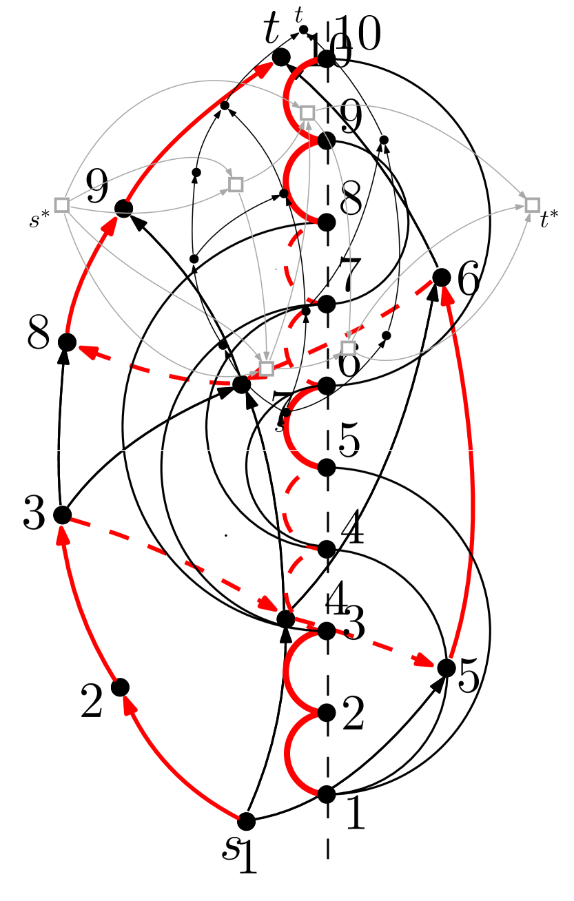
(c)

(d)

Figure 1: (a) A plane $st$-graph $G$. (b) The dual of $G$ is shown in gray. (c) An embedding-preserving HP-completion of $G$. (d) An embedding-preserving $2$UBE $\Gamma$ of $G$ corresponding to (c).

3 NP-Completeness for $\mathbf{k}$UBE ($\mathbf{k\geq 3}$)

We prove that the $k$UBE Testing problem of deciding whether a digraph $G$ admits an upward $k$-page book embedding is NP-complete for each fixed $k\geq 3$. The proof uses a reduction from the Betweenness problem [Opa79].

Betweenness

Instance: A finite set $S$ of elements and a set $R\subseteq S\times S\times S$ of triplets.

Question: Does there exist an ordering $\tau:S\rightarrow\mathbb{N}$ of the elements of $S$ such that for any element $(a,b,c)\in R$ either $\tau(a)<\tau(b)<\tau(c)$ or $\tau(c)<\tau(b)<\tau(a)$?

We incrementally define a set of families of digraphs and prove some properties of these digraphs. Then, we use the digraphs of these families to reduce a generic instance of Betweenness to an instance of 3UBE Testing, thus proving the hardness result for $k=3$. We then explain how the proof can be easily adapted to work for $k>3$.

For a digraph $G$, we denote by $u\leadsto v$ a directed path from a vertex $u$ to a vertex $v$ in $G$. Let $\gamma=\langle\pi,\sigma\rangle$ be a 3UBE of $G$. Two edges $(u,v)$ and $(w,z)$ of $G$ conflict if either $\pi(u)<\pi(w)<\pi(v)<\pi(z)$ or $\pi(w)<\pi(u)<\pi(z)<\pi(v)$. Two conflicting edges cannot be assigned to the same page. The next property will be used in the following; it is immediate from the definition of book embedding and from the pigeonhole principle.

Property 1.

In a 3UBE there cannot exist $4$ edges that mutually conflict.

Shell digraphs.

The first family that we define are the shell digraphs, recursively defined as follows. Digraph $G_{0}$, depicted in Fig. 2(a), consists of a directed path $P$ with $8$ vertices denoted as $s_{0}$, $q_{0}$, $p_{-1}$, $t_{-1}$, $s^{\prime}_{0}$, $q^{\prime}_{0}$, $t^{\prime}_{0}$, and $p_{0}$ in the order they appear along $P$. Besides the edges of $P$, the following directed edges exists in $G_{0}$: $(s_{0},s^{\prime}_{0})$, $(q_{0},q^{\prime}_{0})$, $(t_{-1},p_{0})$. Finally, there is a vertex $t_{0}$ connected to $P$ by means of the two directed edges $(p_{-1},t_{0})$ and $(t^{\prime}_{0},t_{0})$. Graph $G_{h}$ is obtained from $G_{h-1}$ with additional vertices and edges as shown in Fig. 2(b). A new directed path of two vertices $s_{h}$ and $q_{h}$ is connected to $G_{h-1}$ with the edge $(q_{h},s_{h-1})$; a second path of four vertices $s^{\prime}_{h}$, $q^{\prime}_{h}$, $t^{\prime}_{h}$, and $p_{h}$ is connected to $G_{h}$ with the edge $(t_{h-1},s^{\prime}_{h})$. The following edges exist between these new vertices: $(s_{h},s^{\prime}_{h})$, $(q_{h},q^{\prime}_{h})$, $(t_{h-1},p_{h})$. Finally, there is a vertex $t_{h}$ connected to the other vertices by means of the two directed edges $(p_{h-1},t_{h})$ and $(t^{\prime}_{h},t_{h})$. For any $h\geq 0$, the edges $(s_{h},s^{\prime}_{h})$ and $(q_{h},q^{\prime}_{h})$ are called the forcing edges of $G_{h}$; the edges $(p_{h-1},t_{h})$ and $(t_{h-1},p_{h})$ are the channel edges of $G_{h}$; the edge $(t^{\prime}_{h},t_{h})$ is the closing edge of $G_{h}$. The vertices and edges of $G_{h}\setminus G_{h-1}$ are the exclusive vertices and edges of $G_{h}$. The following lemma establishes some basic properties of the shell digraphs.

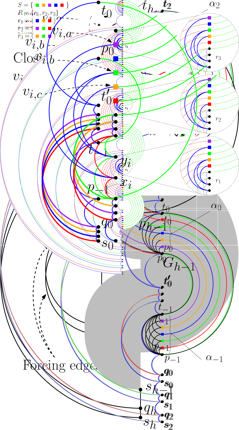
(a) $G_{0}$

(b) $G_{k}$

Figure 2: Definition of shell digraphs. Edges are oriented from bottom to top.

Lemma 1.

Every shell digraph $G_{h}$ for $h\geq 0$ admits a 3UBE. In any 3UBE $\gamma=\langle\pi,\sigma\rangle$ of $G_{h}$ the following conditions hold for every $i=0,1,\dots,h$:

1. all vertices of $G_{i}$ are between $s_{i}$ and $t_{i}$ in $\pi$;

2. the channel edges of $G_{i}$ are in the same page;

3. if $i>0$, the channel edges of $G_{i}$ and those of $G_{i-1}$ are in different pages.

Note that Condition S1 uniquely defines the vertex ordering of $G_{h}$ in every 3UBE. Namely, the path $s_{h}\leadsto p_{0}$ precedes each path $t_{i-1}\leadsto p_{i}$ (for $i=1,\dots,h$), and each path $t_{i-1}\leadsto p_{i}$ precedes the path $t_{i}\leadsto p_{i+1}$ (for $i=1,\dots,h-1$) (see Fig. 3(a) for an example with $h=2$).

(a)

(b)

Figure 3: (a) A 3UBE of the shell digraph $G_{2}$; the colors of the edges represent the pages. (b) Definition of $H_{h,s}$ for $h=2$ and $s=5$. In both figures edges are oriented from bottom to top.

Filled shell digraphs.

Let $G_{h}$ be a shell digraph. A filled shell digraph $H_{h,s}$ (for $h\geq 0$ and $s\geq 1$) is obtained from $G_{h}$ by adding $h+2$ groups $\alpha_{-1},\alpha_{0},\dots,\alpha_{h}$ of $s$ vertices each; see Fig. 3(b) for an illustration. The vertices of group $\alpha_{i}$ are denoted as $v_{i,1},v_{i,2},\dots v_{i,s}$. These vertices will be used to map the elements of the set $S$ of an instance of Betweenness to an instance of 3UBE Testing. For each vertex $v_{-1,j}$ of the set $\alpha_{-1}$ there is a directed edge $(p_{-1},v_{-1,j})$ and a directed edge $(v_{-1,j},t_{-1})$. For each vertex $v_{i,j}$ of the set $\alpha_{i}$ with $i\geq 0$ and $i$ even, there is a directed edge $(p_{i},v_{i,j})$. Finally, for each vertex $v_{i,j}$ of the set $\alpha_{i}$ with $i\geq 0$, there is a directed edge $(v_{i-1,j},v_{i,j})$.

Lemma 2.

Every filled shell digraph $H_{h,s}$ for $s>0$ and even $h\geq 0$ admits a 3UBE. In any 3UBE $\gamma=\langle\pi,\sigma\rangle$ of $H_{h,s}$ the following conditions hold for every $i=-1,0,1,\dots,h$:

1. the vertices of the group $\alpha_{i}$ are between $p_{i}$ and $t_{i}$ in $\pi$;

2. if $i\geq 0$ the vertices of $\alpha_{i}$ are in reverse order with respect to those of $\alpha_{i-1}$ in $\pi$;

3. if $i\geq 0$ each edge $(v_{i-1,j},v_{i,j})$ is in the page of the channel edges of $G_{i}$ (for $j=1,\dots,s$).

Observe that, by Condition F2, all groups $\alpha_{i}$ with even index have the same ordering in $\pi$ and all groups with odd index have the opposite order. As mentioned above the vertices in the groups $\alpha_{i}$ will correspond to the elements of the set $S$ of an instance of Betweenness in the reduced instance of 3UBE Testing. If the reduced instance admits a 3UBE, the order of the groups in $\pi$ will give the desired order for the instance of Betweenness.

$\mathbf{\Lambda}$-filled shell digraphs and hardness proof.

Starting from a filled shell digraph $H_{h,s}$, a $\Lambda$-filled shell digraph $\widehat{H}_{h,s}$ is obtained by replacing some edges with a gadget that has two possible configurations in any 3UBE of $\widehat{H}_{h,s}$. More precisely, we replace each edge $(t^{\prime}_{i},p_{i})$ of $H_{h,s}$ for $i$ odd with the gadget shown in Fig. 4(a). The gadget replacing $(t^{\prime}_{i},p_{i})$ will be denoted as $\Lambda_{i}$. Notice that, this replacement preserves Conditions F1–F3 of Lemma 2.

(a)

(b)

Figure 4: (a) A gadget $\Lambda_{i}$ (black edges). (b) The triplet edges of $G_{i}$ (bold edges).

Lemma 3.

Every $\Lambda$-filled shell digraph $\widehat{H}_{h,s}$ for $s>0$ and even $h\geq 0$ admits a 3UBE. In any 3UBE $\gamma=\langle\pi,\sigma\rangle$ of $\widehat{H}_{h,s}$ the following conditions hold for every $i=1,3,\dots,h-1$:

1. the vertices of the gadget $\Lambda_{i}$ are between $t^{\prime}_{i}$ and $p_{i}$ in $\pi$;

2. the vertices $x_{i}$ and $y_{i}$ are between $w_{i}$ and $z_{i}$ in $\pi$ and there exists a 3UBE $\gamma^{\prime}=\langle\pi^{\prime},\sigma^{\prime}\rangle$ of $\widehat{H}_{h,s}$ where the order of $x_{i}$ and $y_{i}$ is exchanged in $\pi^{\prime}$.

Figure 5: A 3UBE of the $st$-graph $G_{I}$ reduced from a positive instance $I=\langle S,R\rangle$ of Betweenness; the edge colors represent the corresponding pages. Edges are oriented from bottom to top.

Theorem 1.

3UBE Testing is NP-complete even for $st$-graphs.

sketch.

3UBE Testing is clearly in NP. To prove the hardness we describe a reduction from Betweenness. From an instance $I=\langle S,R\rangle$ of Betweenness we construct an instance $G_{I}$ of 3UBE Testing that is an $st$-graph; we start from the $\Lambda$-filled shell digraph $\widehat{H}_{h,s}$ with $h=2|R|$ and $s=|S|$. Let $v_{1},v_{2},\dots,v_{s}$ be the elements of $S$. They are represented in $\widehat{H}_{h,s}$ by the vertices $v_{i,1},v_{i,2},\dots,v_{i,s}$ of the groups $\alpha_{i}$, for $i=-1,0,1,\dots,h$. In the reduction each group $\alpha_{i}$ with odd index is used to encode one triplet and, in a 3UBE of $G_{I}$, the order of the vertices in these groups (which is the same by Condition F2) corresponds to the desired order of the elements of $S$ for the instance $I$. Number the triplets of $R$ from $1$ to $|R|$ and let $(v_{a},v_{b},v_{c})$ be the $j$-th triplet. We use the group $\alpha_{i}$ and the gadget $\Lambda_{i}$ with $i=2j-1$ to encode the triplet $(v_{a},v_{b},v_{c})$. More precisely, we add to $\widehat{H}_{h,s}$ the edges $(x_{i},v_{i,a})$, $(x_{i},v_{i,b})$, $(y_{i},v_{i,b})$, and $(y_{i},v_{i,c})$ (see Fig. 4(b)). These edges are called triplet edges and are denoted as $T_{i}$. In any 3UBE of $G_{I}$ the triplet edges are forced to be in the same page and this is possible if and only if the constraints defined by the triplets in $R$ are respected. The digraph obtained by the addition of the triplet edges is not an $st$-graph because the vertices of the last group $\alpha_{h}$ are all sinks. The desired instance $G_{I}$ of 3UBE Testing is the $st$-graph obtained by adding the edges $(v_{h,j},t_{h})$ (for $j=1,2,\dots,s$). Fig. 5 shows a 3UBE of the $st$-graph $G_{I}$ reduced from a positive instance $I$ of Betweenness.  

For $k>3$, the reduction from an instance $I$ of Betweenness to an instance $G_{I}$ of $k$UBE Testing is similar. In the shell digraph every pair of forcing edges is replaced by a bundle of $k-1$ edges that mutually conflict (see Fig. 6(a)). The edges in each such bundle require $k-1$ pages and force all edges that conflict with them to use the $k$-th page. Analogously, the two edges $(u_{i},z_{i})$ and $(w_{i},p_{i})$ of the gadget $\Lambda_{i}$ are replaced by a bundle of $k-1$ edges that mutually conflict (see Fig. 6(b)); this forces the triplet edges to be in the $k$-th page.

Corollary 1.

$k$UBE Testing is NP-complete for every $k\geq 3$, even for $st$-graphs.

(a)

(b)

Figure 6: Reduction for $k$UBE Testing (example with $k=5$). (a) Replacement of the forcing edges. (b) Replacement of the gadget $\Lambda_{i}$. In both figures colors represent the pages.

4 Existential Results for 2UBE

Let $f$ be an internal face of a plane $st$-graph, and let $p_{l}$ and $p_{r}$ be the left and the right path of $f$; $f$ is a generalized triangle if either $p_{l}$ or $p_{r}$ is a single edge (i.e., a transitive edge), and it is a rhombus if each of $p_{l}$ and $p_{r}$ consists of exactly two edges (see Figs. 7(a) and 7(b)).

Let $G$ be a plane $st$-graph. A forbidden configuration of $G$ consists of a transitive edge $e=(u,v)$ shared by two internal faces $f$ and $g$ such that $s_{f}=s_{g}=u$ and $t_{f}=t_{g}=v$ (i.e., two generalized triangles sharing the transitive edge); see Fig. 7(c). The absence of forbidden configurations is a necessary condition for the existence of an embedding-preserving $2$UBE. If $G$ is triangulated, the absence of forbidden configurations is also a sufficient condition [MS11].

(a)

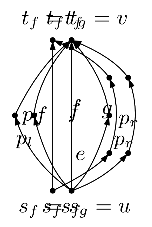
(b)

(c)

Figure 7: (a) A generalized triangle $G$. (b) A rhombus (c) A forbidden configuration.

Theorem 1.

Any plane $st$-graph such that the left and the right path of every internal face contain at least two and three edges, respectively, admits an embedding-preserving $2$UBE.

sketch.

We prove how to construct an embedding-preserving HP-completion. The idea is to construct $\overline{G}$ by adding a face of $G$ per time from left to right, according to a topological ordering of the dual graph of $G$. When a face $f$ is added, its right path is attached to the right boundary of the current digraph. We maintain the invariant that at least one edge $e$ in the left path of $f$ belongs to the Hamiltonian path of the current digraph. The Hamiltonian path is extended by replacing $e$ with a path that traverses the vertices of the right path of $f$. To this aim, dummy edges are suitably inserted inside $f$. When all faces are added, the resulting graph is an HP-completion $\overline{G}$ of $G$. The idea is illustrated in Fig. 8. 

(a)

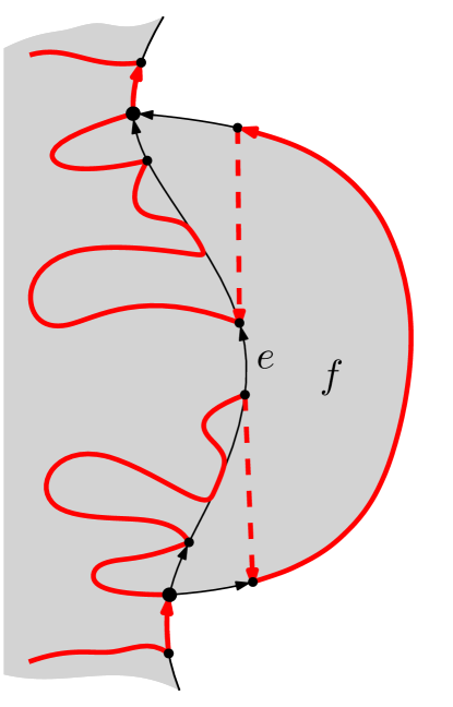
(b)

Figure 8: Idea of the construction in the proof of Theorem 1. Dummy edges are dashed.

The next theorem is proved with a construction similar to that of Theorem 1.

Theorem 2.

Let $G$ be a plane $st$-graph such that every internal face of $G$ is a rhombus. Then $G$ admits an embedding-preserving $2$UBE.

5 Testing 2UBE for Plane Graphs with Special Faces

By Theorem 1, if all internal faces of a plane $st$-graph $G$ are such that their left and right path contain at least two and at least three edges, respectively, $G$ admits an embedding-preserving $2$UBE. If these conditions do not hold, an embedding-preserving $2$UBE may not exist (see Fig. 9(a)). We now describe an efficient testing algorithm for a plane $st$-graph $G=(V,E)$ whose internal faces are generalized triangles or rhombi (see Fig. 9(b)). We construct a mixed graph $G_{M}=(V,E\cup E_{U})$, where $E_{U}$ is a set of undirected edges and $(u,v)\in E_{U}$ if $u$ and $v$ are the two vertices of a rhombus face $f$ distinct from $s_{f}$ and $t_{f}$ (red edges in Fig. 9(c)). For a rhombus face $f$, the graph obtained from $G$ by adding the directed edge $(u,v)$ inside $f$ is still a plane $st$-graph (see, e.g. [BDD⁺18, DETT98]). Since there is only one edge of $E_{U}$ inside each rhombus face of $G$, this implies the following property.

Property 2.

Every orientation of the edges in $E_{U}$ transforms $G_{M}$ into an acyclic digraph.

(a)

(b)

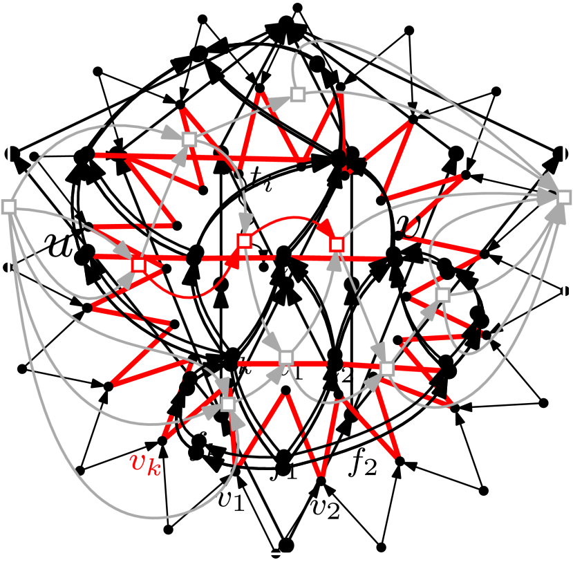
(c)

Figure 9: (a) A plane $st$-graph that does not admit a $2$UBE [NP89]. (b) A plane $st$-graph $G$ whose faces are generalized triangles or rhombi. (b) The mixed graph $G_{M}=(V,E,E_{U})$.

Theorem 1.

Let $G$ be a plane $st$-graph such that every internal face of $G$ is either a generalized triangle or a rhombus. There is an $O(n)$-time algorithm that decides whether $G$ admits an embedding-preserving $2$UBE, and which computes it in the positive case.

Proof.

The edges of $E_{U}$ are the only edges that can be used to construct an embedding-preserving HP-completion of $G$. This, together with Theorem 1, implies that $G$ admits a $2$UBE if and only if the undirected edges of $G_{M}$ can be oriented so that the resulting digraph $\overrightarrow{G_{M}}$ has a directed Hamiltonian path from $s$ to $t$. By Property 2, any orientation of the undirected edges of $G_{M}$ gives rise to an acyclic digraph. On the other hand an acyclic digraph is Hamiltonian if and only if it is unilateral (see, e.g. [ABD⁺18, Theorem 4]); we recall that a digraph is unilateral if each pair of vertices is connected by a directed path (in at least one of the two directions) [MS10]. Testing whether the undirected edges of $G_{M}$ can be oriented so that the resulting digraph $\overrightarrow{G_{M}}$ is unilateral, and computing such an orientation if it exists, can be done in time $O(|V|+|E|+|E_{U}|)=O(n)$ [MS10, Theorem 4]. A Hamiltonian path of $\overrightarrow{G_{M}}$ is given by a topological ordering of its vertices.  

6 Testing Algorithms for 2UBE Parameterized by the Branchwidth

In this section, we show that the $2$UBE Testing problem is fixed-parameter tractable with respect to the branchwidth of the input $st$-graph both in the fixed and in the variable embedding setting. Since the treewidth $tw(G)$ and the branchwidth $bw(G)$ of a graph $G$ are within a constant factor from each other (i.e., $bw(G)-1\leq tw(G)\leq\lfloor\frac{3}{2}bw(G)\rfloor-1$ [RS91]), our FPT algorithm also extends to graphs of bounded treewidth. Previously, the complexity of this problem was settled only for graphs of treewidth at most $2$ in the variable embedding setting [DDLW06].

We use the SPQR-tree data structure [DT96] to efficiently handle the planar embeddings of the input digraphs and sphere-cut decompositions [ST94] to develop a dynamic-programming approach on the skeletons of the rigid components. For the definition of the SPQR-tree $\mathcal{T}$ of a biconnected graph and the related concepts of skeleton $\operatorname{skel}(\mu)$ and pertinent graph $\operatorname{pert}(\mu)$ of a node $\mu$ of $\mathcal{T}$, types of the nodes of $\mathcal{T}$ (namely, S-,P-,Q-, and R-nodes), and virtual edges of a skeleton, see Appendix 0.A. To ease the description, we can assume that each S-node has exactly two children [DGL09] and that the skeleton of each node $\mu$ does not contain the virtual edge representing the parent of $\mu$. In particular, we will exploit the following property of $\mathcal{T}$ when $G$ is an $st$-graph containing the edge $e=(s,t)$ and $\mathcal{T}$ is rooted at the Q-node of $e$.

Property 3 ([DT96]).

Let $\mu\in\mathcal{T}$ with poles $u$ and $v$. Without loss of generality, assume that the directed paths connecting $u$ and $v$ in $G$ are oriented from $u$ to $v$. Then, $\operatorname{pert}(\mu)$ is a $uv$-graph.

For the definition of branchwidth and sphere-cut decomposition, and for the related concepts of middle set $\operatorname{mid}(e)$ and noose $\mathcal{O}_{e}$ of an arc $e$ of the decomposition, and length of a noose, see Appendix 0.A. We denote a sphere-cut decomposition of a plane graph $G=(V,E)$ by the triple $\langle T,\xi,\Pi=\bigcup_{a\in E(T)}\pi_{a}\rangle$, where $T$ is a ternary tree whose leaves are in a one-to-one correspondence with the edges of $G$, which is defined by a bijection $\xi:\mathcal{L}(T)\leftrightarrow E(G)$ between the leaf set $\mathcal{L}(T)$ of $T$ and the edge set $E$, and where $\pi_{a}$ is a circular order of $\operatorname{mid}(a)$, for each arc $a$ of $T$. In particular, we will exploit the property that each of the two subgraphs that lie in the interior and in the exterior of a noose is connected and that the set of nooses forms a laminar set family, that is, any two nooses are either disjoint or nested.

Without loss of generality, we assume that the input $st$-graph $G$ contains the edge $(s,t)$, which guarantees that $G$ is biconnected. In fact, in any $2$UBE of $G$ vertices $s$ and $t$ have to be the first and the last vertex of the spine, respectively. Thus, either $(s,t)$ is an edge of $G$ or it can be added to any of the two pages of the spine of a $2$UBE of $G$ to obtain a $2$UBE $\langle\pi,\sigma\rangle$ of $G\cup(s,t)$. Clearly, the edge $(s,t)$ will be incident to the outer face of $\Gamma(\pi,\sigma)$.

Overview.

Our approach leverages on the classification of the embeddings of each triconnected component of the biconnected graph $G$. Intuitively, such classification is based on the visibility of the spine that the embedding “leaves” on its outer face. We show that the planar embeddings of a triconnected component that yield a $2$UBE of the component can be partitioned into a finite number of equivalence classes, called embedding types. By visiting the SPQR-tree $\mathcal{T}$ of $G$ bottom-up, we describe how to compute all the realizable embedding types of each triconnected component, that is, those embedding types that are allowed by some embedding of the component. To this aim we will exploit the realizable embedding types of its child components. If the root of $\mathcal{T}$, which represents the whole $st$-graph $G$, admits at least one planar embedding belonging to some embedding type, then $G$ admits a $2$UBE. The most challenging part of this approach is handling the triconnected components that correspond to the P-nodes, where the problem is reduced to a maximum flow problem on a capacitated flow network with edge demands, and to the R-nodes, where a sphere-cut decomposition of bounded width is used to efficiently compute the feasible embedding types.

Embedding Types.

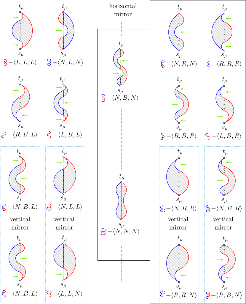
Figure 10: Illustrations of the possible embedding types of a node $\mu$ with poles $s_{\mu}$ and $t_{\mu}$; the portion of the spine that is visible from the left or from the right is green. Pairs of embedding types in the same dotted box are one the vertically-mirrored copy of the other. Embedding types on the top are the horizontally-mirrored copy of the ones on the bottom. Embedding types  -$\langle N,B,N\rangle$ and  -$\langle N,N,N\rangle$ are the horizontal and vertical mirrored copies of themselves.

Given a $2$UBE $\langle\pi,\sigma\rangle$, the two pages will be called the left page (the one to the left of the spine) and the right page (the one to the right of the spine), respectively. We write $\sigma(e)=L$ (resp. $\sigma(e)=R$) if the edge $e$ is assigned to the left page (resp. right page). A point $p$ of the spine is visible from the left (right) page if it is possible to shoot a horizontal ray originating from $p$ and directed leftward (rightward) without intersecting any edge in $\Gamma(\pi,\sigma)$. Let $\mu$ be a node of the SPQR-tree $\cal T$ of $G$ rooted at $(s,t)$. Recall that, by Property 3, since $\cal T$ has been rooted at $(s,t)$, the pertinent graph $\operatorname{pert}(\mu)$ and the skeleton $\operatorname{skel}(\mu)$ of $\mu$ are $s^{\prime}t^{\prime}$-graphs, where $s^{\prime}$ and $t^{\prime}$ are the poles of $\mu$ . We denote by $s_{\mu}$ (by $t_{\mu}$) the pole of $\mu$ that is the source (the sink) of $\operatorname{pert}(\mu)$ and of $\operatorname{skel}(\mu)$. Let $\langle\pi_{\mu},\sigma_{\mu}\rangle$ be a $2$UBE of $\operatorname{pert}(\mu)$ and let $\mathcal{E}_{\mu}$ be the embedding of $\Gamma(\pi_{\mu},\sigma_{\mu})$. We say that $\mathcal{E}_{\mu}$ has embedding type (or is of Type) $\langle s\_{vis},spine\_{vis},t\_{vis}\rangle$ with $s\_{vis},t\_{vis}\in\{L,R,N\}$ and $spine\_{vis}\in\{L,R,B,N\}$ where:

1. $s\_{vis}$ is $L$ (resp., $R$) if in $\mathcal{E}_{\mu}$ there is a portion of the spine incident to $s$ and between $s$ and $t$ that is visible from the left page (resp., from the right page); otherwise, $s\_{vis}$ is $N$.

2. $t\_{vis}$ is $L$ (resp., $R$) if in $\mathcal{E}_{\mu}$ there is a portion of the spine incident to $t$ and between $s$ and $t$ that is visible from the left page (resp., from the right page); otherwise, $t\_{vis}$ is $N$.

3. $spine\_{vis}$ is $L$ (resp., $R$) if in $\mathcal{E}_{\mu}$ there is a portion of the spine between $s$ and $t$ that is visible from the left page (resp., from the right page); $spine\_{vis}$ is $B$ if in $\mathcal{E}_{\mu}$ there is a portion of the spine between $s$ and $t$ that is visible from the left page, and a portion of the spine between $s$ and $t$ that is visible from the right page; otherwise, $spine\_{vis}$ is $N$.

We also say that a node $\mu$ and $\operatorname{pert}(\mu)$ admits Type $\langle x,y,z\rangle$ if $\operatorname{pert}(\mu)$ admits an embedding of Type $\langle x,y,z\rangle$. We have the following lemma.

Lemma 4.

Let $\mu$ be a node of $\cal T$, let $\langle\pi_{\mu},\sigma_{\mu}\rangle$ be a $2$UBE of $\operatorname{pert}(\mu)$ and let $\mathcal{E}_{\mu}$ be a planar embedding of $\Gamma(\pi_{\mu},\sigma_{\mu})$. Then $\mathcal{E}_{\mu}$ has exactly one embedding type, where the possibile embedding types are the $18$ depicted in Fig. 10.

Let $\langle\pi,\sigma\rangle$ be a $2$UBE of $G$, let $\mu$ a node of $\mathcal{T}$, and let $\langle\pi_{\mu},\sigma_{\mu}\rangle$ be the restriction of $\langle\pi,\sigma\rangle$ to $\operatorname{pert}(\mu)$. Further, let $\langle\pi^{\prime}_{\mu},\sigma^{\prime}_{\mu}\rangle\neq\langle\pi_{\mu},\sigma_{\mu}\rangle$ be a $2$UBE of $\operatorname{pert}(\mu)$.

Lemma 5.

If $\langle\pi^{\prime}_{\mu},\sigma^{\prime}_{\mu}\rangle$ and $\langle\pi_{\mu},\sigma_{\mu}\rangle$ have the same embedding type, then $G$ admits a $2$UBE whose restriction to $\operatorname{pert}(\mu)$ is $\langle\pi^{\prime}_{\mu},\sigma^{\prime}_{\mu}\rangle$.

(a) Drawing
$\Gamma(\pi,\sigma)$ of $G$

(b) Drawing
$\Gamma(\pi^{\prime}_{\mu},\sigma^{\prime}_{\mu})$ of $\operatorname{pert}(\mu)$

(c) Drawing $\Gamma^{*}$ of
$G_{\overline{\mu}}\cup\operatorname{pert}(\mu)$

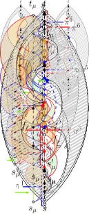
(d) Drawing
$\Gamma^{\prime}$ of $G$

Figure 11: Illustrations for Lemma 5. The $2$UBEs of $\operatorname{pert}(\mu)$ are of Type  -$\langle L,B,N\rangle$.

sketch.

First, insert a possibly squeezed copy of $\Gamma(\pi^{\prime}_{\mu},\sigma^{\prime}_{\mu})$ (Fig. 11(b)) inside $\Gamma(\pi,\sigma)$ (Fig. 11(a)) in the interior of the face $f_{\mu}$ of the plane digraph $G_{\overline{\mu}}$ resulting from removing $\operatorname{pert}(\mu)$ (except its poles) from $\Gamma(\pi,\sigma)$. Second, suitably move parts of the boundary of $f_{\mu}$ along portions of the spine incident to the inserted drawing of $\operatorname{pert}(\mu)$ (Fig. 11(c)). Then, continuously move the copies of the poles of $\mu$ inside $f_{\mu}$ towards their copies in $\Gamma(\pi,\sigma)$, without intersecting any edge, to obtain a drawing $\Gamma^{\prime}$ of $G$ (Fig. 11(d)). 

Recall that, for each node $\mu$ of $\mathcal{T}$, $\operatorname{pert}(\mu)$ may have exponentially many embeddings, given by the permutations of the children of the P-nodes and by the flips of the R-nodes. Lemma 5 is the reason why we only need to compute a single embedding for each embedding type realizable by $\operatorname{pert}(\mu)$, i.e., a constant number of embeddings instead of an exponential number.

We first describe an algorithm to decide if $G$ admits a $2$UBE and its running time. The same procedure can be easily refined to actually compute a $2$UBE of $G$, with no additional cost, by decorating each node $\mu\in\mathcal{T}$ with the embedding choices performed at $\mu$, for each of its $O(1)$ possible embedding types.

Testing Algorithm.

The algorithm is based on computing, for each non-root node $\mu$ of $\mathcal{T}$, the set of embedding types realizable by $\operatorname{pert}(\mu)$, based on whether $\mu$ is an S-, P-, Q-, or an R-node. Since, by Lemmas 4 and 5, $G$ admits a $2$UBE if and only if the pertinent graph of the unique child of the root Q-node admits an embedding of at least one of the $18$ possible embedding types, this approach allows us to solve the $2$UBE Testing problem for $G$.

Recall that the only possible embedding choices for $G$ happen at P- and R-nodes. While the treatment of Q- and S-nodes does not require any modification when considering the variable and the fixed embedding settings, for P- and R-nodes we will discuss how to compute the embedding types that are realizable by $\operatorname{pert}(\mu)$ in both such settings. In particular, in the fixed embedding scenario the above characterization needs to additionally satisfy the constraints imposed by the fixed embedding on the skeletons of the P- and R-nodes in $\mathcal{T}$.

Note that a leaf Q-node only admits embeddings of type  -$\langle L,L,L\rangle$ or  -$\langle R,R,R\rangle$. Also, combining $2$UBEs of the two children of an S-node $\mu$ always yields a $2$UBE of $\operatorname{pert}(\mu)$, whose embedding type can be easily computed. In Section 0.D.1, we prove the following.

Lemma 6.

Let $\mu$ be an S-node. The set of embedding types realizable by $\operatorname{pert}(\mu)$ can be computed in $O(1)$ time, both in the fixed and in the variable embedding setting.

P-nodes.

Let $\mu$ be a P-node with poles $s_{\mu}$ and $t_{\mu}$. Recall that an embedding for a P-node is obtained by choosing a permutation for its children and an embedding type for each child. Our approach to compute the realizable types of $\operatorname{pert}(\mu)$ consists of considering one type at a time for $\mu$. For each embedding type, we check whether the children of $\mu$, together with their realizable embedding types, can be arranged in a finite number of families of permutations (which we prove to be a constant number) so to yield an embedding of the considered type. In order to ease the following description, consider that the arrangements of the children for obtaining some embedding types can be easily derived from the arrangements to obtain the (horizontally) symmetric ones by (i) reversing the left-to-right sequence of the children in the construction and (ii) by taking, for each child, the horizontally-mirrored embedding type; for instance, the arrangements to construct an embedding of Type  -$\langle L,L,N\rangle$ can be obtained from the ones to construct an embedding of Type  -$\langle R,R,N\rangle$, and vice versa. Moreover, two embedding types, namely Type  -$\langle N,B,N\rangle$ and Type  -$\langle N,N,N\rangle$, are (horizontally) self-symmetric. As a consequence, in order to consider all the embedding types that are realizable by $\operatorname{pert}(\mu)$ we describe how to obtain only $10$ “relevant” embedding types (enclosed by a solid polygon in Fig. 10):  -$\langle R,R,R\rangle$,  -$\langle N,R,N\rangle$,  -$\langle R,B,R\rangle$,  -$\langle L,B,R\rangle$,  -$\langle N,R,R\rangle$,  -$\langle N,B,R\rangle$,  -$\langle R,R,N\rangle$,  -$\langle R,B,N\rangle$,  -$\langle N,B,N\rangle$, and  -$\langle N,N,N\rangle$.

Next, we give necessary and sufficient conditions under which the pertinent graph of a P-node admits an embedding of Type  -$\langle N,R,R\rangle$. Then, we show how to test these conditions efficiently by exploiting a suitably defined flow network. The conditions for the remaining types, given in Section 0.D.3, can be tested with the same algorithmic strategy.

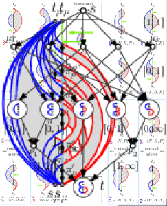
(a)  -$\langle N,R,R\rangle$; Case 1

(b)  -$\langle N,R,R\rangle$; Case 2

(c) Network $\mathcal{N}$ for Case 2

Figure 12: Case 1 (a) and Case 2 (b) of Lemma 7 for a P-nodes $\mu$ of Type  -$\langle N,R,R\rangle$. The spine is colored either green, blue, or black. The green part is the portion of the spine that is visible from the right, the black parts correspond to the bottom-to-top sequences of the internal vertices of $\operatorname{pert}(\mu)$ inherited from the $2$UBEs of the children of $\mu$, the blue parts join sequences inherited from different children. (c) Capacitated flow network $\mathcal{N}$ with edge demands corresponding to (b).

Lemma 7 (Type  -$\langle N,R,R\rangle$).

Let $\mu$ be a P-node. Type  -$\langle N,R,R\rangle$ is admitted by $\mu$ in the variable embedding setting if and only if at least one of two cases occurs. (Case 1) The children of $\mu$ can be partitioned into two parts: The first part consists either of a Type- -$\langle R,R,R\rangle$ Q-node child, or of a Type- -$\langle N,R,R\rangle$ child, or both. The second part consists of any number, even zero, of Type- -$\langle L,B,R\rangle$ children. (Case 2) The children of $\mu$ can be partitioned into three parts: The first part consists either of a Type- -$\langle R,R,R\rangle$ Q-node child, or of a non-Q-node Type- -$\langle R,R,R\rangle$ child, or both. The second part consists of any number, even zero, of Type- -$\langle R,B,R\rangle$ children. The third part consists of any positive number of Type- -$\langle N,B,R\rangle$ or Type- -$\langle L,B,R\rangle$ children, with at most one Type- -$\langle N,B,R\rangle$ child.

Regarding the time complexity of testing the existence of a Type- -$\langle N,R,R\rangle$ embedding of $\operatorname{pert}(\mu)$, we show that deciding if one of (Case 1) or (Case 2) of Lemma 7 applies can be reduced to a network flow problem on a network $\mathcal{N}$ with edge demands. The network for (Case 2) is depicted in Fig. 12(c). The details of this construction are given in Section 0.D.3, where the next lemma is proven.

Lemma 8.

Let $\mu$ be a P-node with $k$ children. The set of embedding types realizable by $\operatorname{pert}(\mu)$ can be computed in $O(k^{2})$ time in the variable embedding setting.

The fixed embedding scenario for a P-node $\mu$ can be addressed by processing the children of $\mu$ in the left-to-right order defined by the given embedding of $G$. The details of such an approach are given in Section 0.D.2, where the following is proven.

Lemma 9.

Let $\mu$ be a P-node with $k$ children. The set of embedding types realizable by $\operatorname{pert}(\mu)$ can be computed in $O(k)$ time in the fixed embedding setting.

Lemmas 6 and 9 yield a counterpart, in the fixed embedding setting, of the linear-time algorithm by Di Giacomo et al. [DDLW06] to compute $2$UBEs of series-parallel graphs.

Theorem 1.

There exists an $O(n)$-time algorithm to decide whether an $n$-vertex series-parallel $st$-graph admits an embedding-preserving $2$UBE.

(a) A sphere-decomposition of $\operatorname{skel}(\mu)\cup(s_{\mu},t_{\mu})$

(b) Outer faces of $\operatorname{skel}_{a_{1}}$ and $\operatorname{skel}_{a_{2}}$

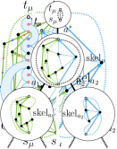
(c) Directed paths of $\operatorname{skel}_{a_{1}}$ and $\operatorname{skel}_{a_{2}}$

(d) Graph $A=A_{1}\cup A_{2}$

Figure 13: Illustrations for the R-node case. (a) A partial sphere-cut decomposition of the graph $\operatorname{skel}(\mu)\cup(s_{\mu},t_{\mu})$ rooted at the edge $(s_{\mu},t_{\mu})$, where $\mu$ is an R-node. The nooses are dotted curves. (b) Outer faces of graphs $\operatorname{skel}_{a_{1}}$ and $\operatorname{skel}_{a_{2}}$. (c) The graphs defined by the directed paths on the outer face of $\operatorname{skel}_{a_{1}}$ and $\operatorname{skel}_{a_{2}}$. (d) The auxiliary graph $A$ for $\operatorname{skel}_{a}$.

R-nodes.

Let $\mu$ be an R-node and $(T,\xi,\Pi)$ be a sphere-cut decomposition of $\operatorname{skel}(\mu)\cup(s_{\mu},t_{\mu})$ of width $\operatorname{\beta}$, rooted at the node $\rho$ with $\xi(\rho)=(s_{\mu},t_{\mu})$; refer to Fig. 13(a). Each arc $a$ of $T$ is associated with a subgraph $\operatorname{skel}_{a}$ of $\operatorname{skel}(\mu)$ and with a subgraph $\operatorname{pert}_{a}$ of $\operatorname{pert}(\mu)$, both bounded by the noose of $a$. Let $a_{1}$ and $a_{2}$ be the two arcs leading to $a$ from the bottom of $T$. Intuitively, our strategy to compute the embedding types of $\operatorname{pert}(\mu)$ is to visit $T$ bottom-up maintaining a succinct description of size $O(\operatorname{\beta})$ of the properties of the $2$UBEs of $\operatorname{pert}_{a}$. To this aim, we construct cycles composed of directed edges that are in one-to-one correspondence with maximal directed paths along the outer face of $\operatorname{skel}_{a_{1}}$ and $\operatorname{skel}_{a_{2}}$ (Figs. 13(b) and 13(c)), which we use to define an auxiliary graph $A$ whose $2$UBEs concisely represent the possible $2$UBEs of $\operatorname{pert}_{a}$ obtained by combining the $2$UBEs of $\operatorname{pert}_{a_{1}}$ and $\operatorname{pert}_{a_{2}}$ (Fig. 13(d)). When we reach the arc $a^{*}$ incident to $\rho$ with $\operatorname{skel}_{a^{*}}=\operatorname{skel}(\mu)$, we use the computed properties to determine the embedding types realizable by $\operatorname{pert}(\mu)$. We provide full details in Section 0.D.4.

Lemma 10.

Let $\mu$ be an R-node whose skeleton $\operatorname{skel}(\mu)$ has $k$ children and branchwidth $\operatorname{\beta}$. The set of embedding types realizable by $\operatorname{pert}(\mu)$ can be computed in $O(2^{O(\operatorname{\beta}\log{\operatorname{\beta}})}\cdot k)$ time, both in the fixed and in the variable embedding setting, provided that a sphere-cut decomposition $\langle T_{\mu},\xi_{\mu},\Pi_{\mu}\rangle$ of width $\beta$ of $\operatorname{skel}^{+}(\mu)$ is given.

By Lemmas 6, 9, 8 and 10 and since $\mathcal{T}$ has $O(|G|)$ size [DT96, DGL09], we get the following.

Theorem 2.

There exists an $O(2^{O(\operatorname{\beta}\log{\operatorname{\beta}})}\cdot n+n^{2}+g(n))$-time algorithm to decide if an $n$-vertex planar (plane) $st$-graph of branchwidth $\operatorname{\beta}$ admits a (embedding-preserving) $2$UBE, where $g(n)$ is the computation time of a sphere-cut decomposition of an $n$-vertex plane graph.

Observe that $g(n)$ is $O(n^{3})$ by the result in [ST94]. Thus, we get the following.

Corollary 2.

There exists an $O(2^{O(\operatorname{\beta}\log{\operatorname{\beta}})}\cdot n+n^{3})$-time algorithm to decide whether an $n$-vertex planar (plane) $st$-graph of branchwidth $\operatorname{\beta}$ admits a (embedding-preserving) $2$UBE.

Since the branchwidth of a planar graph $G$ is at most $2.122\sqrt{n}$ [FT06], Corollary 2 immediately implies that the $2$UBE Testing problem can be solved in sub-exponential time.

Corollary 3.

There exists an $O(2^{O(\sqrt{n}\log{\sqrt{n}})}+n^{3})$-time algorithm to decide whether an $n$-vertex planar (plane) $st$-graph admits a (embedding-preserving) $2$UBE.

7 Conclusion and Open Problems

Our results provide significant advances on the complexity of the $k$UBE Testing problem. We showed NP-hardness for $k\geq 3$; we gave FPT- and polynomial-time algorithms for relevant families of planar $st$-graphs when $k=2$. We point out that our FPT-algorithm can be refined to run in $O(n^{2})$ time for $st$-graphs of treewidth at most $3$, by constructing in linear time a sphere-cut decomposition of their rigid components. We conclude with some open problems.

• The main open question is about the complexity of the $2$UBE Testing problem, which has been conjectured to be NP-complete in the general case [HP99].

• The digraphs in our NP-completeness proof are not upward planar. Since there are upward planar digraphs that do not admit a $3$UBE [Hun89], it would be interesting to study whether the problem remains NP-complete for three pages and upward planar digraphs.

• Finally, it is natural to investigate other families of planar digraphs for which a $2$UBE always exists or polynomial-time testing algorithms can be devised.

Acknowledgments.

This research began at the Bertinoro Workshop on Graph Drawing 2018.

Appendix 0.A Additional Material for Section 2

Connectivity and Planarity.

A graph $G$ is $1$-connected, or simply-connected, if there is a path between any two vertices. $G$ is $k$-connected, for $k\geq 2$, if the removal of $k-1$ vertices leaves the graph $1$-connected. A $2$-connected ($3$-connected) graph is also called biconnected (triconnected).

A planar drawing of $G$ is a geometric representation in the plane such that: $(i)$ each vertex $v\in V(G)$ is drawn as a distinct point $p_{v}$; $(ii)$ each edge $e=(u,v)\in E(G)$ is drawn as a simple curve connecting $p_{u}$ and $p_{v}$; $(iii)$ no two edges intersect in $\Gamma$ except at their common end-vertices (if they are adjacent). A graph is planar if it admits a planar drawing. A planar drawing $\Gamma$ of $G$ divides the plane into topologically connected regions, called faces. The external face of $\Gamma$ is the region of unbounded size; the other faces are internal. A planar embedding of $G$ is an equivalence class of planar drawings that define the same set of (internal and external) faces, and it can be described by the clockwise sequence of vertices and edges on the boundary of each face plus the choice of the external face. Graph $G$ together a given planar embedding is an embedded planar graph, or simply a plane graph: If $\Gamma$ is a planar drawing of $G$ whose set of faces is that described by the planar embedding of $G$, we say that $\Gamma$ preserves this embedding, or also that $\Gamma$ is an embedding-preserving drawing of $G$.

Sphere-cut decomposition.

A branch decomposition $\langle T,\xi\rangle$ of a graph $G=(V,E)$ consists of an unrooted ternary tree $T$ (each node of $T$ has degree one or three) and of a bijection $\xi:\mathcal{L}(T)\leftrightarrow E(G)$ from the leaf set $\mathcal{L}(T)$ of $T$ to the edge set $E(G)$ of $G$. For each arc $a$ of $T$, let $T_{1}$ and $T_{2}$ be the two connected components of $T-a$, and, for $i=1,2$, let $G_{i}$ be the subgraph of $G$ that consists of the edges corresponding to the leaves of $T_{i}$, i.e., the edge set $\{\xi(\mu):\mu\in\mathcal{L}(T)\cap V(T_{i})\}$. The middle set $\operatorname{mid}(a)\subseteq V(G)$ is the intersection of the vertex sets of $G_{1}$ and $G_{2}$, i.e., $\operatorname{mid}(a):=V(G_{1})\cap V(G_{2})$. The width $\operatorname{\beta}(\langle T,\xi\rangle)$ of $\langle T,\xi\rangle$ is the maximum size of the middle sets over all arcs of $T$, i.e., $\operatorname{\beta}(\langle T,\xi\rangle):=max\{|\operatorname{mid}(a)|:a\in T\}$. An optimal branch decomposition of $G$ is a branch decomposition with minimum width; this width is called the branchwidth $\operatorname{\beta}(G)$ of $G$. An optimal branch decomposition of a given planar graph with $n$ vertices can be constructed in $O(n^{3})$ time [ST94].

Let $\Sigma$ be a sphere. A $\Sigma$-plane graph $G$ is a planar graph $G$ embedded (i.e., topologically drawn) on $\Sigma$. A noose of a $\Sigma$-plane graph $G$ is a closed simple curve on $\Sigma$ that (i) intersects $G$ only at vertices and (ii) traverses each face at most once. The length of a noose $O$ is the number of vertices it intersects. Every noose $O$ bounds two closed discs $\Delta_{1}$, $\Delta_{2}$ in $\Sigma$, i.e., $\Delta_{1}\cap\Delta_{2}=O$ and $\Delta_{1}\cup\Delta_{2}=\Sigma$. For a $\Sigma$-plane graph $G$, a sphere-cut decomposition $\langle T,\xi,\Pi=\bigcup_{a\in E(T)}\pi_{a}\rangle$ of $G$ is a branch decomposition $\langle T,\xi\rangle$ of $G$ together with a set $\Pi$ of circular orders $\pi_{a}$ of $\operatorname{mid}(a)$, for each arc $a$ of $T$, such that there exists a noose $O_{a}$ whose closed discs $\Delta_{1}$ and $\Delta_{2}$ enclose the drawing of $G_{1}$ and of $G_{2}$, respectively, for each arc $a$ of $T$. Observe that, $O_{a}$ intersect $G$ exactly at $\operatorname{mid}(a)$ and its length is $|\operatorname{mid}(a)|$. Also, Condition ii of the definition of noose implies that graphs $G_{1}$ and $G_{2}$ are both connected and that the set of nooses forms a laminar set family, that is, any two nooses are either disjoint or nested. A clockwise traversal of $O_{a}$ in the drawing of $G$ defines the cyclic ordering $\pi_{a}$ of $\operatorname{mid}(a)$. We always assume that the vertices of every middle set $\operatorname{mid}(a)=V(G_{1})\cap V(G_{2})$ are enumerated according to $\pi_{a}$. We will exploit the following main result of Dorn et al [DPBF10].

Theorem 1 ([DPBF10],Theorem 1).

Let $G$ be a connected $n$-vertex $\Sigma$-plane graph having branchwidth $\operatorname{\beta}$ and no vertex of degree one. There exists a sphere-cut decomposition of $G$ having width $\operatorname{\beta}$ which can be constructed in $O(n^{3})$ time.

SPQR-trees of Planar $\mathbf{st}$-Graphs.

Let $G$ be a biconnected graph. An SPQR-tree $\mathcal{T}$ of $G$ is a tree-like data structure that represents the decomposition of $G$ into its triconnected components and can be computed in linear time [DT96, GM00, HT73]. See Fig. 14 for an illustration. Each node $\mu$ of $\mathcal{T}$ corresponds to a triconnected component of $G$ with two special vertices, called poles; the triconnected component corresponding to a node $\mu$ is described by a multigraph $\operatorname{skel}(\mu)$ called the skeleton of $\mu$. Let $\operatorname{skel}^{+}(\mu)=\operatorname{skel}(\mu)\cup(u,v)$, where $u$ and $v$ are the poles of $\mu$.ì A node $\mu$ of $\mathcal{T}$ is of one the following types: (i) R-node, if $\operatorname{skel}^{+}(\mu)$ is triconnected; (ii) S-node, if $\operatorname{skel}^{+}(\mu)$ is a cycle of length at least three; (iii) P-node, if $\operatorname{skel}^{+}(\mu)$ is a bundle of at least three parallel edges; and (iv) Q-nodes, if it is a leaf of $\mathcal{T}$; in this case the node represents a single edge of the graph and $\operatorname{skel}^{+}(\mu)$ consists of two parallel edges. A virtual edge in $\operatorname{skel}(\mu)$ corresponds to a tree node $\nu$ adjacent to $\mu$ in $\mathcal{T}$. The edge of $G$ corresponding to the root $\rho$ of $\mathcal{T}$ is the reference edge of $G$, and $\mathcal{T}$ is the SPQR-tree of $G$ with respect to $e$. For every node $\mu\neq\rho$ of $\mathcal{T}$, the subtree $T_{\mu}$ rooted at $\mu$ induces a subgraph $\operatorname{pert}(\mu)$ of $G$ called the pertinent graph of $\mu$, which is described by $T_{\mu}$ in the decomposition: The edges of $\operatorname{pert}(\mu)$ correspond to the Q-nodes (leaves) of $T_{\mu}$.

If $G$ is planar, the SPQR-tree $\mathcal{T}$ of $G$ rooted at a Q-node $\rho$ representing edge $e$ implicitly describes all planar embeddings of $G$ in which $e$ is incident to the outer face. All such embeddings are obtained by combining the different planar embeddings of the skeletons of P- and R-nodes: For a P-node $\mu$, the different embeddings of $\operatorname{skel}(\mu)$ are the different permutations of its edges. If $\mu$ is an R-node, $\operatorname{skel}(\mu)$ has two possible planar embeddings, obtained by flipping $\operatorname{skel}(\mu)$ at its poles. Let $\mu$ be a node of $\mathcal{T}$, let $\mathcal{E}$ be an embedding of $G$, let $\mathcal{E}_{\mu}$ be the embedding $\operatorname{pert}(\mu)$ in $\mathcal{E}$, and let $f^{O}_{\mu}$ be the outer face of $\mathcal{E}_{\mu}$. The path along $f^{O}_{\mu}$ between $s_{\mu}$ and $t_{\mu}$ that leaves $f^{O}_{\mu}$ to its left (resp. to its right) when traversing the boundary of $f^{O}_{\mu}$ from $s_{\mu}$ to $t_{\mu}$ to its the left outer path (resp. the right outer path) of $\mathcal{E}_{\mu}$. The left (resp., right) outer face of $\mathcal{E}_{\mu}$ is the face of $\mathcal{E}$ that is incident to the left (resp., to the right) outer path of $\mathcal{E}_{\mu}$. In Fig. 14(a), the left outer face and the right outer face of the S-node whose poles are the nodes labeled $8$ and $13$ are yellow and green, respectively.

(a)

(b)

Figure 14: (a) A biconnected planar $st$-graph $G$. (b) SPQR-tree of $G$ rooted at the edge $(s,t)$.

Appendix 0.B Additional Material for Section 3

See 1

Proof.

The proof is by induction on $h$.

Base case $h=0$. We describe how to define a 3UBE $\gamma=\langle\pi,\sigma\rangle$ of $G_{0}$. The eight vertices of the directed path $s_{0}\leadsto p_{0}$ must appear in $\pi$ in the same order they appear along the path. Consider now $t_{0}$. Because of the closing edge $(t^{\prime}_{0},t_{0})$, we have $\pi(t^{\prime}_{0})<\pi(t_{0})$. If we put $t_{0}$ between $t^{\prime}_{0}$ and $p_{0}$, the channel edges $(p_{-1},t_{0})$ and $(t_{-1},p_{0})$ and the forcing edges $(s_{0},s^{\prime}_{0})$ and $(q_{0},q^{\prime}_{0})$ would mutually conflict. But then a 3UBE would not exist by Property 1. Thus, the only possibility is that $t_{0}$ is the last vertex in $\pi$. This uniquely defines the order $\pi$ and implies condition S1. As for the page assignment $\sigma$, the two forcing edges must be in different pages because they conflict. Since each of the two channel edges conflict with both forcing edges, the channel edges cannot be assigned to the pages used for the forcing edges. Thus, they must be in the same page, which is possible because the two channel edges do not conflict (this proves condition S2). Finally, the closing edge conflicts with the channel edge $(t_{-1},p_{0})$ and thus it cannot be in the same page as the channel edges; since however it does not conflict with any other edge it can be assigned to one of the pages used for the forcing edges. This concludes the proof that a 3UBE of $G_{0}$ exists and that it must satisfy conditions S1 and S2. Condition S3 does not apply in this case.

Inductive case $h>0$. By induction, $G_{h-1}$ admits a 3UBE $\gamma^{\prime}=\langle\pi^{\prime},\sigma^{\prime}\rangle$ that satisfies S1–S3. We extend $\gamma^{\prime}$ to a 3UBE $\gamma=\langle\pi,\sigma\rangle$ of $G_{h}$ as follows. Since $\gamma^{\prime}$ satisfies S1, $s_{h-1}$ is the first vertex in $\pi^{\prime}$ and $t_{h-1}$ is the last one. The vertices of path $s_{h}\leadsto s_{h-1}$ must appear in $\pi$ in the same order they appear along the path. Analogously, the vertices of $t_{h-1}\leadsto p_{h}$ must appear in $\pi$ in the order they have along the path. Because of the closing edge $(t^{\prime}_{h},t_{h})$, we have $\pi(t^{\prime}_{h})<\pi(t_{h})$. Therefore, $s_{h}$ must be the first vertex along $\pi$. Consider now $t_{h}$. If we put $t_{h}$ between $t^{\prime}_{h}$ and $p_{h}$, the channel edges $(p_{h-1},t_{h})$ and $(t_{h-1},p_{h})$ and the forcing edges $(s_{h},s^{\prime}_{h})$ and $(q_{h},q^{\prime}_{h})$ would mutually conflict. But then a 3UBE would not exist by Property 1. Thus, $t_{h}$ must be the last vertex in $\pi$. This uniquely defines the order $\pi$ and implies condition S1 for $G_{h}$. As for the page assignment $\sigma$, observe that the only exclusive edge of $G_{h}$ that conflicts with some edge of $G_{h-1}$ is the edge $(p_{h-1},t_{h})$, which only conflicts with the channel edge $(p_{h-2},t_{h-1})$ of $G_{h-1}$. This implies that $(p_{h-1},t_{h})$ must be in a page different from the one of $(p_{h-2},t_{h-1})$. The two forcing edges of $G_{h}$ must be in a page different from the channel edge $(p_{h-1},t_{h})$ and since they conflict, they must be in different pages. The channel edge $(t_{h-1},p_{h})$ conflicts with the forcing edges but not with the other channel edge $(p_{h-1},t_{h})$. Thus, the channel edges must be in the same page (which proves condition S2). The fact that the page of $(p_{h-1},t_{h})$ must be different from that of $(p_{h-2},t_{h-1})$, implies condition S3. Finally, the closing edge conflicts with the channel edge $(t_{h-1},p_{h})$ and thus it cannot be in the same page as the channel edges; since however it does not conflict with any other edge, it can be assigned to one of the pages used for the forcing edges. This concludes the proof that a 3UBE of $G_{h}$ exists and that it satisfies conditions S1, S2, and S3.  

See 2

Proof.

The proof is by induction on $h$.

Base case $h=0$. We describe how to define a 3UBE $\gamma=\langle\pi,\sigma\rangle$ of $H_{0,s}$. The subgraph $G_{0}$ of $H_{0,s}$ admits a 3UBE that satisfies conditions S1–S3 by Lemma 1. Let $v_{-1,j}$ (with $1\leq j\leq s$) be a vertex of $\alpha_{-1}$. The edges $(p_{-1},v_{-1,j})$ and $(v_{-1,j},t_{-1})$ imply $\pi(p_{-1})<\pi(v_{-1,j})$ and $\pi(v_{-1,j})<\pi(t_{-1})$, which proves condition F1 for $\alpha_{-1}$. Consider now the group $\alpha_{0}$; the edge $(p_{0},v_{0,j})$ implies $\pi(p_{0})<\pi(v_{0,j})$. On the other hand, if we put $v_{0,j}$ after $t_{0}$, the edge $(v_{-1,j},v_{0,j})$, the channel edge $(p_{-1},t_{0})$, and the two forcing edges $(s_{0},s^{\prime}_{0})$ and $(q_{0},q^{\prime}_{0})$ would mutually conflict. But then a 3UBE would not exist by Property 1. Thus, each vertex of group $\alpha_{0}$ must be between $p_{0}$ and $t_{0}$ in $\pi$, which implies condition F1 for the group $\alpha_{0}$. As for the page assignment $\sigma$, each $(v_{-1,j},v_{0,j})$ conflicts with each forcing edge of $G_{0}$, and thus it must be in the page of the channel edges of $G_{0}$. This implies condition F3. The edges $(v_{-1,j},v_{0,j})$ can be assigned to the same page only if the vertices of $\alpha_{-1}$ appear in reverse order with respect to those of $\alpha_{0}$ in $\pi$. Thus, condition F2 holds and a 3UBE of $H_{0,s}$ can be defined by choosing an arbitrary order for the vertices of $\alpha_{-1}$ and the reverse order for the vertices of $\alpha_{0}$.

Inductive case $h>0$. Consider the subgraph $H^{\prime}_{h,s}$ of $H_{h,s}$ consisting of $H_{h-2,s}$ plus the exclusive vertices and edges of $G_{h}$. By induction and by Lemma 1, $H^{\prime}_{h,s}$ admits a 3UBE $\gamma^{\prime}=\langle\pi^{\prime},\sigma^{\prime}\rangle$ that satisfies conditions F1–F3 and conditions S1–S3. We extend $\gamma^{\prime}$ to a 3UBE $\gamma=\langle\pi,\sigma\rangle$ of $H_{h,s}$ as follows. By condition F1 of $\gamma^{\prime}$, each vertex $v_{h-2,j}$ is before $t_{h-2}$ in $\pi^{\prime}$; on the other hand, because of the edges $(p_{h},v_{h,j})$, each vertex $v_{h,j}$ must follow $p_{h}$ in $\pi$. This implies that each $v_{h-1,j}$ is between $p_{h-1}$ and $t_{h-1}$ in $\pi$. Indeed, if $v_{h-1,j}$ was before $p_{h-1}$ in $\pi$, the edge $(v_{h-1,j},v_{h,j})$, the channel edges $(p_{h-1},t_{h})$ and the two forcing edges of $G_{h}$ would mutually conflict and therefore a 3UBE would not exist by Property 1. On the other hand, if $v_{h-1,j}$ was after $t_{h-1}$, the edge $(v_{h-2,j},v_{h-1,j})$, the channel edges $(p_{h-2},t_{h-1})$ and the two forcing edges of $G_{h-1}$ would mutually conflict and again a 3UBE would not exist by Property 1. Thus, each vertex of group $\alpha_{h-1}$ must be between $p_{h-1}$ and $t_{h-1}$, which proves condition F1 for the group $\alpha_{h-1}$. Consider now a vertex $v_{h,j}$. If it was after $t_{h}$ in $\pi$, then the edge $(v_{h-1,j},v_{h,j})$, the channel edge $(p_{h-1},t_{h})$ and the two forcing edges of $G_{h}$ would mutually conflict – again a 3UBE would not exist by Property 1. Hence, each vertex of $\alpha_{h}$ is between $p_{h}$ and $t_{h}$, which proves condition F1 also for $\alpha_{h}$.

As for the page assignment $\sigma$, each $(v_{h-2,j},v_{h-1,j})$ conflicts with each forcing edge of $G_{h-1}$ and hence it must be in the page of the channel edges of $G_{h-1}$. The same argument applies to the edges $(v_{h-1,j},v_{h,j})$ with respect to the forcing edges of $G_{h}$. Thus the edges $(v_{h-1,j},v_{h,j})$ must be in the page of the channel edges of $G_{h}$, which proves condition F3.

The edges $(v_{h-2,j},v_{h-1,j})$ can be assigned to the same page only if the vertices of $\alpha_{h-2}$ appear in reverse order with respect to those of $\alpha_{h-1}$ in $\pi$. Analogously, the edges $(v_{h-1,j},v_{h,j})$ can be assigned to the same page only if the vertices of $\alpha_{h-1}$ appear in reverse order with respect to those of $\alpha_{h}$ in $\pi$. Thus, condition F2 holds and a 3UBE of $H_{h,s}$ can be defined by ordering the vertices of $\alpha_{h-1}$ in reverse order with respect to those of $\alpha_{h-2}$ and the vertices of $\alpha_{h}$ with the same order as those of $\alpha_{h-2}$.  

See 3

Proof.

By Lemma 2 $H_{h,s}$ admits a 3UBE $\gamma^{\prime}=\langle\pi^{\prime},\sigma^{\prime}\rangle$ where $t^{\prime}_{i}$ and $p_{i}$ are consecutive in $\pi^{\prime}$ for each $i=0,1,\dots,h$. Notice that the gadget $\Lambda_{i}$ admits a 3UBE (actually a 2UBE) $\gamma_{i}$. If we replace the edge $(t^{\prime}_{i},p_{i})$ with $\gamma_{i}$, we do not create any conflict between the edges of $\Lambda_{i}$ and the other edges of $H_{h,s}$. This proves that $\widehat{H}_{h,s}$ has a 3UBE. About condition G1, observe that since any vertex of the gadget $\Lambda_{i}$ belongs to a directed path from $t^{\prime}_{i}$ to $p_{i}$, then the vertices of $\Lambda_{i}$ must be between $t^{\prime}_{i}$ and $p_{i}$. Analogously, $x_{i}$ and $y_{i}$ both appear in a directed path from $w_{i}$ to $z_{i}$ and therefore they must be between $w_{i}$ and $z_{i}$. Suppose that $\pi(x_{i})<\pi(y_{i})$ (the other case is symmetric). If we exchange the order of $x_{i}$ and $y_{i}$ in $\pi^{\prime}$ we introduce a conflict between $(w_{i},x_{i})$ and $(y_{i},z_{i})$, which do not conflict with any other edges. If they are in the same page in $\gamma$ it is sufficient to change the page of one of them in $\gamma^{\prime}$.  

See 1

Proof.

3UBE Testing is clearly in NP. To prove the hardness we describe a reduction from Betweenness. From an instance $I=\langle S,R\rangle$ of Betweenness we construct an instance $G_{I}$ of 3UBE Testing that is an $st$-graph; we start from the $\Lambda$-filled shell digraph $\widehat{H}_{h,s}$ with $h=2|R|$ and $s=|S|$. Let $v_{1},v_{2},\dots,v_{s}$ be the elements of $S$. They are represented in $\widehat{H}_{h,s}$ by the vertices $v_{i,1},v_{i,2},\dots,v_{i,s}$ of the groups $\alpha_{i}$, for $i=-1,0,1,\dots,h$. In the reduction each group $\alpha_{i}$ with odd index is used to encode one triplet and, in a 3UBE of $G_{I}$, the order of the vertices in these groups (which is the same by condition F2) corresponds to the desired order of the elements of $S$ for the instance $I$. Number the triplets of $R$ from $1$ to $|R|$ and let $(v_{a},v_{b},v_{c})$ be the $j$-th triplet. We use the group $\alpha_{i}$ and the gadget $\Lambda_{i}$ with $i=2j-1$ to encode the triplet $(v_{a},v_{b},v_{c})$. More precisely, we add to $\widehat{H}_{h,s}$ the edges $(x_{i},v_{i,a})$, $(x_{i},v_{i,b})$, $(y_{i},v_{i,b})$, and $(y_{i},v_{i,c})$ (see Fig. 4(b)). These edges are called triplet edges and are denoted as $T_{i}$. In any 3UBE of $G_{I}$ the triplet edges are forced to be in the same page and this is possible if and only if the constraints defined by the triplets in $R$ are respected. The digraph obtained by the addition of the triplet edges is not an $st$-graph because the vertices of the last group $\alpha_{h}$ are all sinks. The desired instance $G_{I}$ of 3UBE Testing is the $st$-graph obtained by adding the edges $(v_{h,j},t_{h})$ (for $j=1,2,\dots,s$). Fig. 5 shows a 3UBE of the $st$-graph $G_{I}$ reduced from a positive instance $I$ of Betweenness.

We now show that $I$ is a positive instance of Betweenness if and only if the $st$-graph $G_{I}$ constructed as described above admits a 3UBE. Suppose first that $I$ is a positive instance of Betweenness, i.e., there exists an ordering $\tau$ of $S$ that satisfies all triplets in $R$. The subgraph $\widehat{H}_{h,s}$ of $G_{I}$ admits a 3UBE that satisfies conditions S1–S3, F1–F3, and G1–G2 by Lemmas 1, LABEL:, 2, LABEL: and 3. Observe that the order of the vertices of the groups $\alpha_{i}$ can be arbitrarily chosen (provided that all groups with even index have the same order and the groups with odd index have the reverse order). Thus we can choose the order of the groups with odd index to be equal to $\tau$. Let $\gamma=\langle\pi,\sigma\rangle$ be the resulting 3UBE of $\widehat{H}_{h,s}$. We now show that if we add the triplet edges to $\gamma$, these edges do not conflict. Let $(v_{a},v_{b},v_{c})$ be the triplet encoded by the triplet edges $T_{i}$ and suppose that $\tau(v_{a})<\tau(v_{b})<\tau(v_{c})$ (the other case is symmetric). Since the vertices of the groups with odd index are ordered in $\pi$ as in $\tau$, we have $\pi(v_{i,a})<\pi(v_{i,b})<\pi(v_{i,c})$. If $\pi(x_{i})<\pi(y_{i})$ then the edges $T_{i}$ do not conflict. If otherwise $\pi(y_{i})<\pi(x_{i})$, by condition G2 we can exchange the order of $x_{i}$ and $y_{i}$, thus guaranteeing again that the triplet edges $T_{i}$ do not conflict. On the other hand, the triplet edges $T_{i}$ conflict with the edges $E^{\Lambda}_{i}$ of $\Lambda_{i}$, with the channel edges $E^{ch}_{i}$ of $G_{i}$, and with all the edges $E^{\alpha}_{i}$ connecting group $\alpha_{i-1}$ to group $\alpha_{i}$. All the edges in $E^{\Lambda}_{i}\cup E^{ch}_{i}\cup E^{\alpha}_{i}$ can be assigned to only two pages. Indeed, the edges $E^{\Lambda}_{i}$ require two pages, while one page is enough for the edges of $E^{ch}_{i}\cup E^{\alpha}_{i}$. Also, since the edges of $E^{\Lambda}_{i}$ do not conflict with those in $E^{ch}_{i}\cup E^{\alpha}_{i}$, two pages suffice for all of them. Hence, the triplet edges $T_{i}$ can all be assigned to the third page. Since this is true for all the triplet edges, $G_{I}$ admits a 3UBE.

Suppose now that $G_{I}$ admits a 3UBE $\gamma=\langle\pi,\sigma\rangle$. By Lemmas 1, LABEL:, 2, LABEL: and 3 $\gamma$ satisfies conditions S1–S3, F1–F3, and G1–G2 . By condition F2 the order of the vertices of the groups $\alpha_{i}$ with odd index is the same for all groups. We claim that all triplets in $R$ are satisfied if this order is used as the order $\tau$ for the elements of $S$. Let $(v_{a},v_{b},v_{c})$ be the triplet encoded by the triplet edges $T_{i}$. By condition G2, the vertices $x_{i}$ and $y_{i}$ of the gadget $\Lambda_{i}$ are between $w_{i}$ and $z_{i}$ in $\pi$. Thus the triplet edges $T_{i}$ conflict with the edges $(u_{i},z_{i})$ and $(w_{i},p_{i})$. These two edges must be in two different pages because they conflict. It follows that the triplet edges $T_{i}$ must all be in the same page, i.e., the third one. Since the three edges of $T_{i}$ are in the same page we have either $\pi(x_{i})<\pi(y_{i})$ and $\pi(v_{i,a})<\pi(v_{i,b})<\pi(v_{i,c})$ or $\pi(y_{i})<\pi(x_{i})$ and $\pi(v_{i,c})<\pi(v_{i,b})<\pi(v_{i,a})$ (any other order would cause a crossing between the edges of $T_{i}$). In both cases vertex $v_{i,b}$ is between $v_{i,a}$ and $v_{i,c}$, i.e., $v_{b}$ is between $v_{a}$ and $v_{c}$ in $\tau$. Since this is true for all triplets, $I$ is a positive instance of Betweenness.  

Appendix 0.C Additional Material for Section 4

See 1

Proof.

We prove how to construct an HP-completion. The idea is to construct $\overline{G}$ by adding a face of $G$ per time from left to right. Namely, the faces of $G$ are added according to a topological ordering of the dual graph of $G$. When a face $f$ is added, its right path is attached to the right boundary of the current digraph. We maintain the invariant that at least one edge $e$ in the left path of $f$ belongs to the Hamiltonian path of the current digraph. The Hamiltonian path is extended by replacing $e$ with a path that traverses the vertices of the right path of $f$. To this aim, dummy edges are suitably inserted inside $f$. When all faces are added, the resulting graph is an HP-completion $\overline{G}$ of $G$.

More precisely, let $G^{*}$ be the dual graph of $G$. Let $s^{*}=f_{0},f_{1},\dots,f_{N},f_{N+1}=t^{*}$ be a topological sorting of $G^{*}$. Denote by $G_{0}$ the left boundary of $G$ and by $G_{i}$, for $i=1,2,\dots,N$, the subgraph of $G$ consisting of the faces $f_{1},f_{2},\dots,f_{i}$. $G_{i}$ can be obtained by adding the right path $p^{i}_{r}$ of face $f_{i}$ to $G_{i-1}$. We construct a sequence $\overline{G}_{0},\overline{G}_{1},\dots,\overline{G}_{N}$ of $st$-graphs such that $\overline{G}_{i}$ is an HP-completion of $G_{i}$. Clearly, $\overline{G}_{N}$ will be an HP-completion of $G$. While constructing the sequence, we maintain the following invariant: given any two consecutive edges along the right boundary of $\overline{G}_{i}$, at least one of them belongs to the Hamiltonian path $P_{\overline{G}_{i}}$ of $\overline{G}_{i}$. $\overline{G}_{0}$ coincides with $G_{0}$ and all its edges are in $P_{\overline{G}_{0}}$, so the invariant holds. Suppose then that $\overline{G}_{i-1}$, with $i>1$, satisfies the invariant. To construct $\overline{G}_{i}$ we must add the right path $p^{i}_{r}$ of $f_{i}$ plus possibly some dummy edges inside $f_{i}$. Let $s_{f}=v_{0},v_{1},v_{2},\dots,v_{k-1},t_{f}=v_{k}$ be the right path $p^{i}_{r}$ of $f_{i}$ and let $s_{f}=u_{0},u_{1},u_{2},\dots,u_{h-1},t_{f}=u_{h}$ be the left path $p^{i}_{l}$ of $f_{i}$. By hypothesis $p^{i}_{r}$ has at least three edges, and therefore $k\geq 3$; moreover, since $G$ has no transitive edge, $h\geq 2$. Notice that $p^{i}_{l}$ is a subpath of the right boundary of $\overline{G}_{i-1}$ and that the right boundary of $\overline{G}_{i}$ is obtained from the right boundary of $\overline{G}_{i-1}$ by replacing $p^{i}_{l}$ with $p^{i}_{r}$. Let $(u_{-1},s_{f})$ be the edge along the right boundary of $\overline{G}_{i-1}$ entering $s_{f}$ and let $(t_{f},u_{h+1})$ be the edge along the right boundary of $\overline{G}_{i-1}$ exiting $t_{f}$. We have different cases depending on whether $(u_{-1},s_{f})$ and $(t_{f},u_{h+1})$ belong to $P_{\overline{G}_{i-1}}$ or not.

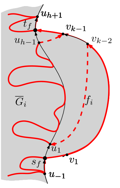
(a)

(b)

Figure 15: Illustration for the proof of Theorem 1: Case 1.

Case 1: both $(u_{-1},s_{f})$ and $(t_{f},u_{h+1})$ belong to $P_{\overline{G}_{i-1}}$. See Fig. 15 for an illustration. By the invariant there is an edge $(u_{j},u_{j+1})$ with $0\leq j\leq h-1$ between $s_{f}$ and $t_{f}$ that belongs to $P_{\overline{G}_{i-1}}$. We add the two dummy edges $(u_{j},v_{1})$ and $(v_{k-1},u_{j+1})$, thus “extending” $P_{\overline{G}_{i-1}}$ to a Hamiltonian path $P_{\overline{G}_{i}}$ of $\overline{G}_{i}$; namely, the edge $(u_{j},u_{j+1})$ is bypassed by the path $u_{j},v_{1},v_{2},\dots,v_{k-1},u_{j+1}$. The only edges of $p^{i}_{r}$ that do not belong to $P_{\overline{G}_{i}}$ are $(s_{f},v_{1})$ and $(v_{k-1},t_{f})$. Since $(u_{-1},s_{f})$ and $(t_{f},u_{h+1})$ belong to $P_{\overline{G}_{i-1}}$ they also belong to $P_{\overline{G}_{i}}$ and thus the invariant is preserved.

(a)

(b)

Figure 16: Illustration for the proof of Theorem 1: Case 2.

Case 2: $(u_{-1},s_{f})$ belongs to $P_{\overline{G}_{i-1}}$, while $(t_{f},u_{h+1})$ does not. See Fig. 16 for an illustration. By the invariant the edge $(u_{h-1},t_{f})$ belongs to $P_{\overline{G}_{i-1}}$. We add the dummy edge $(u_{h-1},v_{1})$. This“extends” $P_{\overline{G}_{i-1}}$ to $P_{\overline{G}_{i}}$ of $\overline{G}_{i}$ bypassing the edge $(u_{h-1},t_{f})$ with the path $u_{h-1},v_{1},v_{2},\dots,v_{k-1},t_{f}$. The only edge of $p^{i}_{r}$ that does not belong to $P_{\overline{G}_{i}}$ is $(s_{f},v_{1})$. Since $(u_{-1},s_{f})$ belong to $P_{\overline{G}_{i-1}}$ it also belongs to $P_{\overline{G}_{i}}$ and thus the invariant is preserved.

Case 3: $(u_{-1},s_{f})$ does not belongs to $P_{\overline{G}_{i-1}}$, while $(t_{f},u_{h+1})$ does. This case is symmetric to the previous one.

(a)

(b)

Figure 17: Illustration for the proof of Theorem 1: Case 4.

Case 4: neither $(u_{-1},s_{f})$ nor $(t_{f},u_{h+1})$ belong to $P_{\overline{G}_{i-1}}$. See Fig. 17 for an illustration. By the invariant the edges $(s_{f},u_{1})$ $(u_{h-1},t_{f})$ belong to $P_{\overline{G}_{i-1}}$. We add the two dummy edges $(v_{k-2},u_{1})$ and $(u_{h-1},v_{k-1})$. In this case we “extend” $P_{\overline{G}_{i-1}}$ to $P_{\overline{G}_{i}}$ bypassing $(s_{f},u_{1})$ with the path $s_{f},v_{1},\dots,v_{k-2}$ and bypassing the edge $(u_{h-1},t_{f})$ with the path $u_{h-1},v_{k-1},t_{f}$. The only edge of $p^{i}_{r}$ that does not belong to $P_{\overline{G}_{i}}$ is $(v_{k-2},v_{k-1})$; moreover, the two edges $(s_{f},v_{1})$ and $(v_{k-1},t_{f})$ belong to $P_{\overline{G}_{i}}$. Thus the invariant is preserved.  

See 2

Proof.

The statement can be proved using the same technique as in the proof of Theorem 1. If all faces are rhombi, when we construct $\overline{G}_{i}$ from $\overline{G}_{i-1}$, we have that $p^{i}_{l}$ is a path $s_{f},u_{1},t_{f}$ and $p^{i}_{r}$ is a path $s_{f},v_{1},t_{f}$. One between $(s_{f},u_{1})$ and $(u_{1},t_{f})$ belongs to $P_{\overline{G}_{i-1}}$. If $(s_{f},u_{1})$ belongs to $P_{\overline{G}_{i-1}}$ we add the dummy edge $(v_{1},u_{1})$. In this case we bypass the edge $(s_{f},u_{1})$ with the path $s_{f},v_{1},u_{1}$. If $(u_{1},t_{f})$ belongs to $P_{\overline{G}_{i-1}}$ we add the dummy edge $(u_{1},v_{1})$. In this case we bypass the edge $(u_{1},t_{f})$ with the path $u_{1},v_{1},t_{f}$. In both cases it is easy to see that the invariant is maintained.  

Appendix 0.D Additional Material for Section 6

See 4

Proof.

The first statement follows from the definition of embedding type. To see that the number of embedding types allowed by $\operatorname{pert}(\mu)$ is at most $18$ it suffices to consider the following facts. First, the number of different embedding types allowed by $\operatorname{pert}(\mu)$ is at most $36$. Further, some combinations are “impossible”, in the sense that not all combinations of values for $s\_{vis}$, $spine\_{vis}$, and $t\_{vis}$ appear in a $2$UBE. In particular, we have that following values for $spine\_{vis}$ are forbidden: (a) $spine\_{vis}$cannot be $L$, if either $s\_{vis}=R$ or $t\_{vis}=R$; (b) $spine\_{vis}$cannot be $R$, if either $s\_{vis}=L$ or $t\_{vis}=L$; (c) $spine\_{vis}$cannot be $N$, if either $s\_{vis}$ or $t\_{vis}$ is different from $N$. Condition a rules out $5$ combinations; Condition b and Condition c rule out $5$ and $8$ more combinations, respectively. This leaves us with $18$ embedding types; see Fig. 10.  

See 5

Proof.

We show how to construct a $2$UBE $\langle\pi^{\prime},\sigma^{\prime}\rangle$ of $G$ whose restriction to $\operatorname{pert}(\mu)$ is $\langle\pi^{\prime}_{\mu},\sigma^{\prime}_{\mu}\rangle$. For the ease of description we actually show how to construct an upward planar drawing $\Gamma^{\prime}$ of $G$ in which each vertex $v$ lies along the spine in the same bottom-to-top order determined by $\pi^{\prime}$ and each edge is drawn on the page assigned by $\sigma^{\prime}$. Clearly, such a drawing implies the existence of $\langle\pi^{\prime},\sigma^{\prime}\rangle$.

Consider the canonical drawing $\Gamma(\pi,\sigma)$ of $G$; refer to Fig. 11(a). Consider the drawing $\Gamma_{\overline{\mu}}$ of $G_{\overline{\mu}}$ obtained by restricting $\Gamma(\pi,\sigma)$ to the edges of $G$ not in $\operatorname{pert}(\mu)$ and to their endpoints. Denote by $\pi_{\overline{\mu}}$ the bottom-to-top order of the vertices of $G_{\overline{\mu}}$ in $\Gamma_{\overline{\mu}}$. Let $\pi_{1},\pi_{2},\dots,\pi_{k}$ be the maximal subsequences of $\pi_{\overline{\mu}}$ between $s_{\mu}$ and $t_{\mu}$ and composed of consecutive vertices in $\pi_{\overline{\mu}}$ that are also consecutive in $\pi$ (refer to Fig. 11(a)). Observe that sequences $\pi_{i}$, $i=1,\dots,k$, may be formed by a single vertex or by multiple vertices. Also, the first sequence $\pi_{1}$ includes $s_{\mu}$ and the last sequence $\pi_{k}$ includes $t_{\mu}$. Further, unless $\operatorname{pert}(\mu)$ is an edge, for which the statement is trivial, we have that $k\geq 3$.

Drawing $\Gamma_{\overline{\mu}}$ contains a face $f_{\mu}$ that is incident to $s_{\mu}$, $t_{\mu}$, and all the starting and ending vertices of the sequences $\pi_{i}$, with $i=2,\dots,k-1$. In particular, some starting and ending vertices of the sequences $\pi_{i}$ are encountered when traversing $f_{\mu}$ clockwise from $s_{\mu}$ to $t_{\mu}$ (left vertices of $f_{\mu}$) and some of them are encountered when traversing $f_{\mu}$ counter-clockwise from $s_{\mu}$ to $t_{\mu}$ (right vertices of $f_{\mu}$).

We show how to insert into face $f_{\mu}$ the drawing $\Gamma(\pi^{\prime}_{\mu},\sigma^{\prime}_{\mu})$ of $\operatorname{pert}(\mu)$, producing the promised drawing $\Gamma^{\prime}$ of the $2$UBE $\langle\pi^{\prime},\sigma^{\prime}\rangle$ of $G$.

First, consider the drawing $\Gamma(\pi^{\prime}_{\mu},\sigma^{\prime}_{\mu})$ of $\operatorname{pert}(\mu)$ (see Fig. 11(b)) and insert it, possibly after squeezing it, into $f_{\mu}$ in such a way that its spine lays entirely on the line of the spine of $\Gamma_{\overline{\mu}}$ and in such a way that the vertices of $\mu$ do not fall in between the vertices of any maximal sequence $\pi_{i}$, $i=1,\dots,k$. This is always possible since $k\geq 3$ and, therefore, there exists a portion of the spine of $\Gamma_{\overline{\mu}}$ which is in the interior of $f_{\mu}$. Observe that this implies that $s_{\mu}$ and $t_{\mu}$ have now a double representation, since the drawing of the source $s^{\prime}_{\mu}$ and sink $t^{\prime}_{\mu}$ of $\Gamma(\pi^{\prime}_{\mu},\sigma^{\prime}_{\mu})$ do not coincide with the drawing of $s_{\mu}$ and $t_{\mu}$ in $\Gamma_{\overline{\mu}}$. Denote by $\Gamma^{*}$ the resulting drawing.

Suppose $\langle\pi_{\mu},\sigma_{\mu}\rangle$ (and, hence, also $\langle\pi^{\prime}_{\mu},\sigma^{\prime}_{\mu}\rangle$) has Type $\langle x,y,z\rangle$. Observe that if $y\in\{N,R\}$ then there are no left vertices of $f_{\mu}$. Otherwise, if $y\in\{L,B\}$, then it is possibile to identify two vertices $v_{\ell,b}$ and $v_{\ell,t}$ of $\Gamma(\pi^{\prime}_{\mu},\sigma^{\prime}_{\mu})$ such that a portion of the spine is visible from the left between $v_{\ell,b}$ and $v_{\ell,t}$. Move between $v_{\ell,b}$ and $v_{\ell,t}$ on the spine in $\Gamma^{*}$ all the vertices of the sequences $\pi_{i}$ whose starting and ending vertices are left vertices of $f_{\mu}$, preserving their relative order. Analogously, observe that if $y\in\{N,L\}$, then there are no right vertices of $f_{\mu}$. Otherwise, if $y\in\{R,B\}$, then it is possibile to identify two vertices $v_{r,b}$ and $v_{r,t}$ of $\Gamma(\pi^{\prime}_{\mu},\sigma^{\prime}_{\mu})$ such that a portion of the spine is visible from the left between $v_{r,b}$ and $v_{r,t}$. Move between $v_{r,b}$ and $v_{r,t}$ on the spine in $\Gamma^{*}$ all the vertices of the sequences $\pi_{i}$ whose starting and ending vertices are right vertices of $f_{\mu}$, preserving their relative order. Refer to Fig. 11(c).

Observe that in $\Gamma^{*}$ the edges of $G$ lie in the pages prescribed by $\sigma^{\prime}$ by construction. Also, in $\Gamma^{*}$ the bottom-to-top order of the vertices is the same as $\pi^{\prime}$ with the exception of the two duplicates vertices $s^{\prime}_{\mu}$ and $t^{\prime}_{\mu}$. Thus, by identifying $s_{\mu}$ with $s^{\prime}_{\mu}$ and $t_{\mu}$ with $t^{\prime}_{\mu}$, we obtain the promised upward drawing $\Gamma^{\prime}$ of $G$ in which each vertex $v$ lies along the spine in the same bottom-to-top order determined by $\pi^{\prime}$ and each edge is drawn as a $y$-monotone curve on the page assigned by $\sigma^{\prime}$. To complete the proof we argue about the planarity of $\Gamma^{\prime}$. Clearly, identifying $s_{\mu}$ with $s^{\prime}_{\mu}$ ($t_{\mu}$ with $t^{\prime}_{\mu}$) does not introduce crossings when $s_{\mu}$ with $s^{\prime}_{\mu}$ ($t_{\mu}$ with $t^{\prime}_{\mu}$) are consecutive along the spine in $\Gamma^{*}$ (see $t^{\prime}_{\mu}$ and $t_{\mu}$ in Fig. 11(c)). In the case in which $s_{\mu}$ and $s^{\prime}_{\mu}$ ($t_{\mu}$ and $t^{\prime}_{\mu}$) are not consecutive along the spine in $\Gamma^{*}$, necessarily $x\in\{L,R\}$ ($z\in\{L,R\}$). Suppose $x=L$ ($z=L$), the case when $x=R$ ($z=R$) being analogous. There cannot exist in $\Gamma_{\overline{\mu}}$ an edge $e=(a,b)$ such that $\pi(a)<\pi(s_{\mu})<\pi(b)$ and such that $\sigma(e)=R$. Therefore, we can continuously move $s^{\prime}_{\mu}$, together with its incident edges, toward $s_{\mu}$, remaining inside the region bounded by $f_{\mu}$ without intersecting any edge of $G_{\overline{\mu}}$ (see Fig. 11(d)). This concludes the proof.  

0.D.1 S-nodes

See 6

Proof.

Let $\mu$ be an S-node with poles $s_{\mu}$ and $t_{\mu}$. Let $\mu^{\prime}$ and $\mu^{\prime\prime}$ be the two children of $\mu$ with poles $s_{\mu^{\prime}}$, $t_{\mu^{\prime}}$ and $s_{\mu^{\prime\prime}}$, $t_{\mu^{\prime\prime}}$, respectively, where $s_{\mu^{\prime}}=s_{\mu}$, $t_{\mu^{\prime}}=s_{\mu^{\prime\prime}}$, and $t_{\mu^{\prime\prime}}=t_{\mu}$. Clearly, combining each pair of $2$UBEs of the two children of $\mu$ always yields a $2$UBE of $\operatorname{pert}(\mu)$. Let $\langle x^{\prime},y^{\prime},x^{\prime}\rangle$ and $\langle x^{\prime\prime},y^{\prime\prime},z^{\prime\prime}\rangle$ be the embedding types of $2$UBEs of $\operatorname{pert}(\mu^{\prime})$ and $\operatorname{pert}(\mu^{\prime\prime})$, respectively. The embedding type $\langle x,y,z\rangle$ of the $2$UBE of $\operatorname{pert}(\mu)$ resulting from combining such $2$UBEs can be computed as follows. We have $x=x^{\prime}$ and $z=z^{\prime}$. As for $y$, we have that: (i) $y=N$iff $y^{\prime}=y^{\prime\prime}=N$; (ii) $y=L$if either $y^{\prime}=L$ and $y^{\prime\prime}\in\{L,N\}$ or $y^{\prime\prime}=L$ and $y^{\prime}\in\{L,N\}$; (iii) $y=R$if either $y^{\prime}=R$ and $y^{\prime\prime}\in\{R,N\}$ or $y^{\prime\prime}=R$ and $y^{\prime}\in\{R,N\}$; (iv) $y=B$if at least one of $y^{\prime}$ and $y^{\prime\prime}$ is $B$ or one of them is $L$ and the other is $R$.  Since the number of embedding types realizable by the two children of $\mu$ is constant, the statement follows.  

0.D.2 P-nodes: Fixed Embedding

Let $\mu$ be a P-node with poles $s_{\mu}$ and $t_{\mu}$ and let $\mu_{1},\mu_{2},\dots,\mu_{k}$ be the children of $\mu$ in the left-to-right order defined by the given embedding of $G$.

Let $\operatorname{skel}^{i}(\mu)$ and $\operatorname{pert}^{i}(\mu)$ be the subgraphs of $\operatorname{skel}(\mu)$ and of $\operatorname{pert}(\mu)$, respectively, determined by children $\mu_{1},\mu_{2},\dots,\mu_{i}$ of $\mu$. Clearly, the embedding types that are realizable by $\operatorname{pert}^{1}(\mu)$ are those that are realizable by $\operatorname{pert}(\mu_{1})$. For $i=2,\dots,k$, we can compute the set $X_{i}$ of embedding types that are realizable by $\operatorname{pert}^{i}(\mu)$ as follows. We consider each embedding type $\langle x,y,z\rangle\in X_{i-1}$ and each embedding type $\langle a,b,c\rangle$ that is realizable by $\operatorname{pert}(\mu_{i})$, and we either determine that no embedding type can be obtained by composing the pair $\langle x,y,z\rangle$ and $\langle a,b,c\rangle$ or compute an embedding type $\langle p,q,w\rangle$ for $\operatorname{pert}^{i}(\mu)$, which we add to $X_{i}$, as follows.

Rejection:

If $x\in\{N,L\}$ and $a\in\{N,R\}$, then we reject the pair. Similarly, if $z\in\{N,L\}$ and $c\in\{N,R\}$, then we reject the pair. If $y=L$, then we reject the instance, as $\operatorname{pert}(\mu_{i})$ contains at least an internal vertex that has to be placed on the spine to the left of $\operatorname{pert}^{i-1}(\mu_{i})$ and between $s_{\mu}$ and $t_{\mu}$.

Embedding Types for $\operatorname{pert}^{i}{\mu}$:

If $x=a$, then $p=x$, and if $x=N$ or $a=N$, then $p=N$. Similarly, if $z=c$, then $w=z$, and if $z=N$ or $c=N$, then $w=N$. If $y=L$ and $b\in\{R,B\}$, then $q=B$; also, if $y=L$ and $b=L$, then $q=L$. Similarly, if $y=R$ and $b\in\{L,B\}$, then $q=B$; also, if $y=R$ and $b=R$, then $q=R$. Finally, if $y=B$ and $b\in\{R,B\}$, then $q=B$; if $y=B$ and $b=L$, then $q=L$.

Since the set of rules above defines the set $X_{k}$ of embedding types realizable by $\operatorname{pert}(\mu)$ and the above computations can easily be performed in time linear in the number of children of $\mu$, we obtain Lemma 9.

0.D.3 P-nodes: Variable Embedding

In this section, we give necessary and sufficient conditions under which a P-node $\mu$ admits one of the relevant embedding types (enclosed by a solid polygon in Fig. 10) in the variable embedding setting. We start with the conditions for Type  -$\langle N,R,R\rangle$ and discuss the time complexity of testing such conditions.

See 7

Proof.

The necessity can be argued by considering that all children must be of Type $\langle\cdot,\cdot,R\rangle$ and at most one child can be of Type $\langle N,\cdot,\cdot\rangle$.

For the sufficiency, we consider the two cases separately. In (Case 1) we order the children of $\mu$ so that from left to right we have the possible Q-node child, if any, followed by the unique Type- -$\langle N,R,R\rangle$ child, followed by the Type- -$\langle L,B,R\rangle$ children in any order; see Fig. 12(a). In (Case 2) we order the children of $\mu$ so that from left to right we have the possible Type- -$\langle R,R,R\rangle$ Q-node child, if any, followed by the possible non-Q-node Type- -$\langle R,R,R\rangle$ child, followed by the Type- -$\langle R,B,R\rangle$ children in any order, followed by the possible Type- -$\langle N,B,R\rangle$, if any, followed by the Type- -$\langle L,B,R\rangle$ children in any order, if any; see Fig. 12(b).

We show that the ordering $\mu_{1},\mu_{2},\dots,\mu_{k}$ of the children of $\mu$ described in the two cases above determines a $2$UBE of $\operatorname{pert}(\mu)$.

Denote with $\langle\pi_{i},\sigma_{i}\rangle$ the $2$UBE of $\operatorname{pert}(\mu_{i})$, where $\pi_{i}$ is the bottom-to-top ordering of the internal vertices of $\operatorname{pert}(\mu_{i})$ in the $2$UBE and where $\sigma_{i}:E(\operatorname{pert}(\mu_{i}))\rightarrow\{R,L\}$ is the assignment of the edges of $\operatorname{pert}(\mu_{i})$ to the two pages of the $2$UBE. In (Case 1) we construct a $2$UBE $\langle\pi,\sigma\rangle$ of $\operatorname{pert}(\mu)$ as follows: see Fig. 12(a) for an example. The bottom-to-top ordering $\pi$ of the vertices of $\operatorname{pert}(\mu)$ is $s_{\mu},\pi_{1},\pi_{2},\dots,\pi_{k},t_{\mu}$. The assignment $\sigma$ of the edges of $\operatorname{pert}(\mu)$ to the two pages is the one determined by the $\sigma_{i}$‘s, that is, $\sigma(e)=\sigma_{i}(e)$ if $e\in\operatorname{pert}(\mu_{i})$. Further, if edge $(s_{\mu},t_{\mu})$ exists, then $\sigma\big{(}(s_{\mu},t_{\mu})\big{)}=L$. Clearly, $\langle\pi,\sigma\rangle$ is of a $2$UBE of $\operatorname{pert}(\mu)$ of Type  -$\langle N,R,R\rangle$. In (Case 2) we construct a $2$UBE $\langle\pi,\sigma\rangle$ of $\operatorname{pert}(\mu)$ as follows: see Fig. 12(b) for an example. Observe that the children of $\mu$ of Type  -$\langle R,B,R\rangle$ or Type  -$\langle N,B,R\rangle$ determine a consecutive subsequence $\mu_{p},\dots,\mu_{q}$ of the left-to-right sequence of the children of $\mu$, with $2\leq p\leq q\leq k$. For each child $\mu_{i}$, $i=p,\dots,q$, by the definition of Type  -$\langle R,B,R\rangle$ and Type  -$\langle N,B,R\rangle$, there exist two consecutive vertices $v^{\prime}$ and $v^{\prime\prime}$ in $\pi_{i}$ such that portion of the spine between them is visible from the left. Therefore, we can split $\pi_{i}$ into two subsequences $\pi^{\prime}_{i}$ and $\pi^{\prime\prime}_{i}$ where $v^{\prime}\in\pi^{\prime}_{i}$ and $v^{\prime\prime}\in\pi^{\prime\prime}_{i}$. We construct $\langle\pi,\sigma\rangle$ as follows. Let $\mu^{*}$ be the possible Type- -$\langle R,R,R\rangle$ child of $\mu$. The bottom-to-top ordering $\sigma$ of the vertices of $\operatorname{pert}(\mu)$ in the $2$UBE is $s_{\mu},\pi^{\prime}_{p},\pi^{\prime}_{p+1},\dots,\pi^{\prime}_{q},\pi^{*},$ $\pi^{\prime\prime}_{q},\pi^{\prime\prime}_{q-1},\dots,\pi^{\prime\prime}_{p},\pi_{q+1},\dots\pi_{k},t_{\mu}$, where $\pi^{*}=\emptyset$ if $\mu^{*}$ does not exist. The assignment $\sigma$ of the edges of $\operatorname{pert}(\mu)$ to the pages of the $2$UBE is the one determined by the $\sigma_{i}$‘s. Further, if edge $(s_{\mu},t_{\mu})$ exists, then $\sigma\big{(}(s_{\mu},t_{\mu})\big{)}=L$. Clearly, $\langle\pi,\sigma\rangle$ is of a $2$UBE of $\operatorname{pert}(\mu)$ of Type  -$\langle N,R,R\rangle$.  

Regarding the computational complexity of deciding if one of (Case 1) or (Case 2) of Lemma 7 applies, we show that such a task can be reduced to a network flow problem on a network $\mathcal{N}$ with edge demands.

We describe the construction of $\mathcal{N}$ for (Case 2) (refer to Figs. 12(b) and 12(c)); the construction for (Case 1) being similar. Network $\mathcal{N}$ is a capacitated flow network where each arc $e$ has a label $[l,u]$, where $l$ is a lower bound and $u$ is an upper bound on the flow traversing $e$ in a feasible flow. In particular, $\mathcal{N}$ contains a source $s$; a sink $t$; a node $\mu_{i}$ for each child $\mu_{i}$ of $\mu$; a node $t\in\{\mbox{\raisebox{-2.0pt}{\includegraphics[page=19,height=10.0pt,width=5.0pt]{icons.pdf}}\hskip 1.0pt-$\langle R,R,R\rangle$},\mbox{\raisebox{-2.0pt}{\includegraphics[page=5,height=10.0pt,width=5.0pt]{icons.pdf}}\hskip 1.0pt-$\langle R,R,R\rangle$},\mbox{\raisebox{-2.0pt}{\includegraphics[page=3,height=10.0pt,width=7.0pt]{icons.pdf}}\hskip 1.0pt-$\langle R,B,R\rangle$},\mbox{\raisebox{-2.0pt}{\includegraphics[page=7,height=10.0pt,width=7.0pt]{icons.pdf}}\hskip 1.0pt-$\langle N,B,R\rangle$},\mbox{\raisebox{-2.0pt}{\includegraphics[page=1,height=10.0pt,width=7.0pt]{icons.pdf}}\hskip 1.0pt-$\langle L,B,R\rangle$}\}$, representing each embedding type used in constructing the sequence of (Case 2); and two special nodes $\nu_{1}$ and $\nu_{2}$. Network $\mathcal{N}$ contains the following arcs: $(s,\mu_{i})$ with label $[1,1]$, for $i=1,\dots,k$; an arc $(\mu_{i},t)$ with label $[0,1]$, for each type $t$ for which $\operatorname{pert}(\mu_{i})$ admits a Type-$t$ $2$UBE; an arc $(\mbox{\raisebox{-2.0pt}{\includegraphics[page=19,height=10.0pt,width=5.0pt]{icons.pdf}}\hskip 1.0pt-$\langle R,R,R\rangle$},\nu_{1})$ with label $[0,1]$; an arc $(\mbox{\raisebox{-2.0pt}{\includegraphics[page=5,height=10.0pt,width=5.0pt]{icons.pdf}}\hskip 1.0pt-$\langle R,R,R\rangle$},\nu_{1})$ with label $[0,1]$; an arc $(\nu_{1},t)$ with label $[1,2]$; an arc $(\mbox{\raisebox{-2.0pt}{\includegraphics[page=3,height=10.0pt,width=7.0pt]{icons.pdf}}\hskip 1.0pt-$\langle R,B,R\rangle$},t)$ with label $[0,\infty]$; an arc $(\mbox{\raisebox{-2.0pt}{\includegraphics[page=3,height=10.0pt,width=7.0pt]{icons.pdf}}\hskip 1.0pt-$\langle R,B,R\rangle$},\nu_{2})$ with label $[0,1]$; an arc $(\mbox{\raisebox{-2.0pt}{\includegraphics[page=1,height=10.0pt,width=7.0pt]{icons.pdf}}\hskip 1.0pt-$\langle L,B,R\rangle$},\nu_{2})$ with label $[0,\infty]$; and an arc $(\nu_{2},t)$ with label $[1,\infty]$. Observe that $\mathcal{N}$ has size linear in the number $k$ of children of $\mu$ due to the fact that the outdegree of $\mu_{i}$ nodes is bounded by the number of embedding types, $s$ has outdegree $k$, and the remaining nodes have outdegree at most $1$.

Clearly, a sequence corresponding to (Case 2) exists if and only if the network $\mathcal{N}$ admits a feasible flow, which has value $k$. Testing the existence of a feasible flow can be reduced in linear time to a maxflow problem in a suitable capacitated network $\mathcal{N}^{\prime}$ [KT06]. We obtain a solution by applying the standard max-flow algorithm by Ford–Fulkerson, which runs in $O(|E(\mathcal{N})|\times f)$, where $f$ is the value of the maximum flow.

Next, we give the conditions for the remaining relevant embedding types  -$\langle R,R,R\rangle$,  -$\langle N,R,N\rangle$,  -$\langle R,B,R\rangle$,  -$\langle L,B,R\rangle$,  -$\langle N,B,R\rangle$,  -$\langle R,R,N\rangle$,  -$\langle R,B,N\rangle$,  -$\langle N,B,N\rangle$, and  -$\langle N,N,N\rangle$, whose testing can be carried out with the same algorithmic strategy as for Type  -$\langle N,R,R\rangle$. Altogether, we obtain Lemma 8.

Lemma 11 (Type  -$\langle L,B,R\rangle$).

Let $\mu$ be a P-node. Type  -$\langle L,B,R\rangle$ is admitted by $\mu$ in the variable embedding setting if and only if all of its children admit Type  -$\langle L,B,R\rangle$.

Proof.

For the necessity, consider any $2$UBE $\mathcal{E}$ of $\operatorname{pert}(\mu)$ of Type  -$\langle L,B,R\rangle$. Let $\mu^{*}$ be any child of $\mu$ and let $\mathcal{E}^{*}$ be the $2$UBE of $\operatorname{pert}(\mu^{*})$ obtained by restricting $\mathcal{E}$ to $\operatorname{pert}(\mu^{*})$. It is immediate that there exist a portion of the spine incident to $s_{\mu}$ and between $s_{\mu}$ and $t_{\mu}$ that is visible from the left page and a portion of the spine incident to $t_{\mu}$ and between $s_{\mu}$ and $t_{\mu}$ that is visible from the right page. Thus, $\mu$ admits Type  -$\langle L,B,R\rangle$. For the sufficiency, we order the children of $\mu$ arbitrarily; see Fig. 18(a) for an example. Clearly, the resulting embedding of $\operatorname{pert}(\mu)$ is of Type  -$\langle L,B,R\rangle$.

(a)  -$\langle L,B,R\rangle$

(b)  -$\langle R,B,R\rangle$

(c)  -$\langle R,R,R\rangle$; Case 1

(d)  -$\langle R,R,R\rangle$; Case 2

Figure 18: Constructions for P-nodes of Type  -$\langle L,B,R\rangle$,  -$\langle R,B,R\rangle$, and  -$\langle R,R,R\rangle$.

Lemma 12 (Type  -$\langle R,B,R\rangle$).

Let $\mu$ be a P-node. Type  -$\langle R,B,R\rangle$ is admitted by $\mu$ in the variable embedding setting if and only if all of its children admit Type  -$\langle R,B,R\rangle$.

Proof.

Both the necessity and sufficiency proofs follow the same line as the proofs for Lemma 11; see Fig. 18(b) for an example.  

Lemma 13 (Type  -$\langle R,R,R\rangle$).

Let $\mu$ be a P-node. Type  -$\langle R,R,R\rangle$ is admitted by $\mu$ in the variable embedding setting if and only if one of these two cases occurs: (Case 1) There exists a Q-node $\omega$ corresponding to edge $(s_{\mu},t_{\mu})$ between the poles of $\mu$, all the other children of $\mu$ except for at most one node $\xi$ admit Type  -$\langle R,B,R\rangle$, and $\xi$, if it exists, admits Type  -$\langle R,R,R\rangle$. (Case 2) Edge $(s_{\mu},t_{\mu})$ between the poles of $\mu$ does not exist, there exists a child $\xi$ of $\mu$ admitting Type  -$\langle R,R,R\rangle$, and all the other children of $\mu$, if any, admit Type  -$\langle R,B,R\rangle$.

Proof.

It is easy to see that these conditions are necessary: in fact, for any child $\mu_{i}$ of $\mu$, the restriction of a Type- -$\langle R,R,R\rangle$ embedding of $\operatorname{pert}(\mu)$ to $\operatorname{pert}(\mu_{i})$ is clearly of Type $\langle R,X,R\rangle$, with $X\in\{R,B\}$. Also, an embedding of Type  -$\langle R,R,R\rangle$ for $\operatorname{pert}(\mu)$ is incompatible with more than one embedding of Type  -$\langle R,R,R\rangle$ for its children unless one of them is a single edge. If no child has embedding of Type  -$\langle R,R,R\rangle$, then $\mu$ would have Type  -$\langle R,B,R\rangle$. For the sufficiency, we consider the two cases separately. Let $\mu_{1},\dots,\mu_{k}$ be the non-Q-node children of $\mu$. In (Case 1) we order the children of $\mu$ so that from left to right we have node $\omega$, followed by $\xi$, if any, followed by the remaining children of $\mu$; see Fig. 18(c). In (Case 2) we order the children of $\mu$ so that from left to right we have node $\xi$ followed by the remaining children of $\mu$; see Fig. 18(d).  

Lemma 14 (Type  -$\langle N,B,R\rangle$).

Let $\mu$ be a P-node. Type  -$\langle N,B,R\rangle$ is admitted by $\mu$ in the variable embedding setting if and only if at least one of these two cases occurs: (Case 1) All children admit either Type  -$\langle L,B,R\rangle$ or Type  -$\langle R,B,R\rangle$, and there exists at least a Type- -$\langle L,B,R\rangle$ child and a Type- -$\langle R,B,R\rangle$ child. (Case 2) There exists a Type- -$\langle N,B,R\rangle$ child and all other children admit either Type  -$\langle L,B,R\rangle$ or Type  -$\langle R,B,R\rangle$.

Proof.

It is easy to see that these conditions are necessary. In fact, for any child $\mu_{i}$ of $\mu$, the restriction of a Type- -$\langle N,B,R\rangle$ embedding of $\operatorname{pert}(\mu)$ to $\operatorname{pert}(\mu_{i})$ is clearly of Type $\langle X,Y,R\rangle$, with $X\in\{R,L,N\}$ and $Y=B$ since an embedding of $\mu$ with $pocket_{side}=B$ implies an embedding of all its children with $pocket_{side}=B$.

For the sufficiency, in both cases we order the children from left to right in such a way that Type- -$\langle R,B,R\rangle$ children precede all the Type- -$\langle L,B,R\rangle$ children; see Figs. 19(a) and 19(b). In (Case 2) the  -$\langle N,B,R\rangle$ child is placed between the last Type- -$\langle R,B,R\rangle$ child e the first Type- -$\langle L,B,R\rangle$ child; see Fig. 19(b).

(a)  -$\langle N,B,R\rangle$; Case 1

(b)  -$\langle N,B,R\rangle$; Case 2

Figure 19: Constructions for P-nodes of Type  -$\langle N,B,R\rangle$.

Lemma 15 (Type  -$\langle R,B,N\rangle$).

Let $\mu$ be a P-node. Type  -$\langle R,B,N\rangle$ is admitted by $\mu$ in the variable embedding setting if and only if at least one of two cases occurs, which can be obtained from (Case 1) and (Case 2) discussed for Type  -$\langle N,B,R\rangle$ (Lemma 14) by considering the types of its children after a vertical flip, i.e., we replace each Type-$\langle X,Y,Z\rangle$ child with a Type-$\langle Z,Y,X\rangle$ child.

Proof.

The necessity and sufficiency proofs are symmetric to those presented in Lemma 14.  

Lemma 16 (Type  -$\langle N,B,N\rangle$).

Let $\mu$ be a P-node. Type  -$\langle N,B,N\rangle$ is admitted by $\mu$ in the variable embedding setting if and only if at least one of six cases occur. Since Type  -$\langle N,B,N\rangle$ is self-symmetric, we have that, for each case, we can obtain a symmetric one by reversing the left-to-right sequence of the children in the construction and by taking, for each child, the horizontally-mirrored embedding Type. Thus, for each pair of symmetric cases, we only describe one. (Case 1) There exists a child that admits Type  -$\langle N,B,N\rangle$ and the other children admit either Type  -$\langle R,B,R\rangle$ or Type  -$\langle L,B,L\rangle$. (Case 2) It is possible to partition the children of $\mu$ into three parts as follows. The first part consists of any positive number of Type- -$\langle R,B,R\rangle$ or Type- -$\langle N,B,R\rangle$ children, with at most one Type- -$\langle N,B,R\rangle$ child. The second part consists of any number, even zero, of Type- -$\langle L,B,R\rangle$ children. The third part consists of any positive number of Type- -$\langle L,B,N\rangle$ or Type- -$\langle L,B,L\rangle$ children, with at most one Type- -$\langle L,B,N\rangle$ child. (Case 3) This case is obtained from Case 2 by considering the types of its children after a vertical flip.

Proof.

For the sufficiency, we consider the three cases separately. In (Case 1) we order the children of $\mu$ so that from left to right we have the Type- -$\langle R,B,R\rangle$ children, if any, in any order, followed by the unique Type- -$\langle N,B,N\rangle$ child, followed by the Type- -$\langle L,B,L\rangle$ children, if any, in any order; see Fig. 20(a). In (Case 2) we order the children of $\mu$ so that from left to right we have the possible Type- -$\langle R,B,R\rangle$ children, if any, in any order, followed by the possible Type- -$\langle N,B,R\rangle$ child, if any, followed by the possible Type- -$\langle L,B,R\rangle$, if any, in any order, followed by the possible Type- -$\langle L,B,N\rangle$ child, if any, followed by the possible Type- -$\langle L,B,L\rangle$ children, if any, in any order (see Fig. 20(b)). In (Case 3) we proceed as in (Case 2) by considering the types after a vertical flip. Clearly, these orderings allow for a $2$UBE of $\operatorname{pert}(\mu)$.

The necessity can be argued by considering that at most one child can be of Type $\langle N,\cdot,\cdot\rangle$, at most one child can be of Type $\langle\cdot,\cdot,N\rangle$, and any child must be of Type $\langle\cdot,B,\cdot\rangle$.

(a)  -$\langle N,B,N\rangle$; Case 1

(b)  -$\langle N,B,N\rangle$; Case 2

Figure 20: Constructions for P-nodes of Type  -$\langle N,B,N\rangle$.

Lemma 17 (Type  -$\langle R,R,N\rangle$).

Let $\mu$ be a P-node. Type  -$\langle R,R,N\rangle$ is admitted by $\mu$ in the variable embedding setting if and only if at least one of two cases occurs, which can be obtained from (Case 1) and (Case 2) discussed for Type  -$\langle N,R,R\rangle$ (Lemma 7) by considering the types of its children after a vertical flip.

Proof.

The necessity and sufficiency proofs are symmetric to those presented in Lemma 7.  

Lemma 18 (Type  -$\langle N,R,N\rangle$).

Let $\mu$ be a P-node. Type  -$\langle N,R,N\rangle$ is admitted by $\mu$ in the variable embedding setting if and only if at least one of these six cases occurs: (Case 1) There exists a child that admits Type  -$\langle N,R,N\rangle$ and the other non-Q-node children admit Type  -$\langle L,B,L\rangle$. (Case 2) It is possible to partition the children of $\mu$ into three parts as follows. The first part consists of at least one child of Type  -$\langle R,R,R\rangle$ of which at most one is not a Q-node. The second part consists of any number, even zero, of Type- -$\langle R,B,R\rangle$ children. The third part consists of any positive number of Type- -$\langle N,B,N\rangle$ or Type- -$\langle L,B,L\rangle$ children, with at most one Type- -$\langle N,B,N\rangle$ child. (Case 3) It is possible to partition the children of $\mu$ into three parts as follows. The first part consists of at least one and at most two children of distinct types, namely, a Type- -$\langle R,R,R\rangle$ Q-node and a Type- -$\langle R,R,N\rangle$ child. The second part consists of any number, even zero, of Type- -$\langle R,B,L\rangle$ children. The third part consists of any positive number of Type- -$\langle N,B,L\rangle$ or Type- -$\langle L,B,L\rangle$ children, with at most one Type- -$\langle N,B,L\rangle$ child. (Case 4) This case is obtained from the previous one by considering the types of the children of $\mu$ after a vertical flip. (Case 5) It is possible to partition the children of $\mu$ into three parts as follows. The first part consists of at least one child of Type  -$\langle R,R,R\rangle$ of which at most one is not a Q-node. The second part consists of any number, even zero, of children of Type  -$\langle R,B,N\rangle$ or Type  -$\langle R,B,L\rangle$, with at most one Type- -$\langle R,B,N\rangle$ child. The third part consists of any positive number of Type- -$\langle N,B,L\rangle$ or Type- -$\langle L,B,L\rangle$ children, with at most one Type- -$\langle N,B,L\rangle$ child. (Case 6) This case is obtained from the previous one by considering the types of the children of $\mu$ after a vertical flip.

Proof.

For the sufficiency, we consider the six cases separately. In (Case 1) we order the children of $\mu$ so that from left to right we have the Type- -$\langle R,R,R\rangle$ Q-node child, if any, followed by the unique Type- -$\langle N,R,N\rangle$ child, followed by the Type- -$\langle L,B,L\rangle$ children, if any, in any order; see Fig. 21(a). In (Case 2) we order the children of $\mu$ so that from left to right we have the Type- -$\langle R,R,R\rangle$ Q-node child, if any, followed by the Type- -$\langle R,R,R\rangle$ non-Q-node child, if any, followed by the Type  -$\langle R,B,R\rangle$ children, if any, in any order, followed by the unique Type- -$\langle N,B,N\rangle$ child, if any, followed by the Type- -$\langle L,B,L\rangle$ children, if any, in any order; see Fig. 21(b). In (Case 3) we order the children of $\mu$ so that from left to right we have the Type- -$\langle R,R,R\rangle$ Q-node child, if any, followed by the Type- -$\langle R,R,N\rangle$ child, if any, followed by the Type  -$\langle R,B,L\rangle$ children, if any, in any order, followed by the unique Type- -$\langle N,B,L\rangle$ child, if any, followed by the Type- -$\langle L,B,L\rangle$ children, if any, in any order; see Fig. 21(c). In (Case 4) we proceed as in (Case 3) by considering the types after a vertical flip. In (Case 5) we order the children of $\mu$ so that from left to right we have the Type- -$\langle R,R,R\rangle$ Q-node child, if any, followed by the Type- -$\langle R,R,R\rangle$ non-Q-node child, if any, followed by the Type- -$\langle R,B,N\rangle$ child, if any, followed by the Type  -$\langle R,B,L\rangle$ children, if any, in any order, followed by the unique Type- -$\langle N,B,L\rangle$ child, if any, followed by the Type- -$\langle L,B,L\rangle$ children, if any, in any order; see Fig. 21(d). In (Case 6) we proceed as in (Case 5) by considering the types after a vertical flip.

The necessity can be argued by considering that at most one child can be of Type $\langle N,\cdot,\cdot\rangle$, at most one child can be of Type $\langle\cdot,\cdot,N\rangle$, and that any child must be of Type $\langle\cdot,R,\cdot\rangle$ or of Type $\langle\cdot,B,\cdot\rangle$. However, not all the children of $\mu$ may be of Type $\langle\cdot,B,\cdot\rangle$ as otherwise the resulting embeddings would be of Type $\langle\cdot,B,\cdot\rangle$.

(a)  -$\langle N,R,N\rangle$; Case 1

(b)  -$\langle N,R,N\rangle$; Case 2

(c)  -$\langle N,R,N\rangle$; Case 3

(d)  -$\langle N,R,N\rangle$; Case 5

Figure 21: Constructions for P-nodes of Type  -$\langle N,R,N\rangle$.

Lemma 19 (Type  -$\langle N,N,N\rangle$).

Let $\mu$ be a P-node. Type  -$\langle N,N,N\rangle$ is admitted by $\mu$ in the variable embedding setting if and only if at least one of $26$ cases occurs. Since Type  -$\langle N,N,N\rangle$ is self-symmetric, for each pair of symmetric cases, we only describe one. Further, we assume that Case $i$ applies only if Case $1$, Case $2$, …, Case $i-1$ do not apply. (Case 1) There exist exactly two children, one of which is a Type- -$\langle R,R,R\rangle$ Q-node and the other is a Type- -$\langle N,N,N\rangle$ node. (Case 2) There exists exactly one Type- -$\langle N,R,N\rangle$ child, at least one and at most two Type- -$\langle R,R,R\rangle$ children of which at most one is a non-Q-node child, and all the remaining children are of Type  -$\langle L,B,L\rangle$. (Case 3) It is possible to partition the children of $\mu$ into five parts as follows. The first part consists of at least one and at most two Type- -$\langle R,R,R\rangle$ children of which at most one is a non-Q-node child. The second part consists of any number of Type- -$\langle R,B,R\rangle$ children. The third part consists of exactly one Type- -$\langle N,B,N\rangle$ child. The fourth part consists of any number of Type- -$\langle L,B,L\rangle$ children. The fifth part consists of at least one and at most two Type- -$\langle L,L,L\rangle$ children of which at most one is a non-Q-node child. (Case 4) There exists exactly one Type- -$\langle R,R,N\rangle$ child, any number of Type- -$\langle R,B,L\rangle$ and Type- -$\langle L,B,L\rangle$ children, at most one Type- -$\langle N,B,L\rangle$ child, and at least one and at most two Type- -$\langle L,L,L\rangle$ children of which at most one is a non-Q-node child. (Case 5) This case is obtained from the previous one by considering the types of the children of $\mu$ after a vertical flip. (Case 6) There exists exactly one Type- -$\langle R,R,N\rangle$ child, any number of Type- -$\langle R,B,L\rangle$ children, at most one Type- -$\langle N,L,L\rangle$ child, and at least one child that is either a Type- -$\langle N,L,L\rangle$ child or it is a Q-node Type- -$\langle L,L,L\rangle$ child. (Case 7) This case is obtained from the previous one by considering the types of the children of $\mu$ after a vertical flip. (Case 8) There exists exactly one Type- -$\langle R,B,N\rangle$ child, at most one Type- -$\langle N,B,L\rangle$ child, any number of Type- -$\langle R,B,R\rangle$, Type- -$\langle R,B,L\rangle$, and Type- -$\langle L,B,L\rangle$ children. Further, there exist at least one and at most two non-Q-node children of distinct types between Type  -$\langle R,R,R\rangle$ and Type  -$\langle L,L,L\rangle$, where if only one of such children exists then $\mu$ has also a Q-node child. (Case 9) This case is obtained from the previous one by considering the types of the children of $\mu$ after a vertical flip. (Case 10) There exists exactly one Type- -$\langle R,B,N\rangle$ child, any number of Type- -$\langle R,B,R\rangle$ and Type- -$\langle R,B,L\rangle$ children. Further, there exist at least one and at most two non-Q-node children of distinct types between Type  -$\langle R,R,R\rangle$ and Type  -$\langle N,L,L\rangle$, where if only one of such children exists then $\mu$ has also a Q-node child. (Case 11) This case is obtained from the previous one by considering the types of the children of $\mu$ after a vertical flip. (Case 12) There exists exactly one non-Q-node Type- -$\langle R,R,R\rangle$ child, any number of Type- -$\langle R,B,R\rangle$ and Type- -$\langle L,B,R\rangle$ children, and at least one and at most two Type- -$\langle L,L,L\rangle$ children of which at most one is a non-Q-node child. (Case 13) This case is obtained from the previous one by considering the types of the children of $\mu$ after a vertical flip.

Proof.

(a)  -$\langle N,N,N\rangle$; Case 1

(b)  -$\langle N,N,N\rangle$; Case 2

(c)  -$\langle N,N,N\rangle$; Case 3

(d)  -$\langle N,N,N\rangle$; Case 3

Figure 22: Constructions for P-nodes of Type  -$\langle N,N,N\rangle$. Subfigures (c) and (d) show the constructions for Case 3 when there exists no Type- -$\langle R,R,R\rangle$ non-Q-node child and when there exists such a child, respectively.

We consider the three cases separately. In (Case 1) we order the children of $\mu$ so that from left to right we have the Type- -$\langle R,R,R\rangle$ Q-node child followed by the Type- -$\langle N,N,N\rangle$ child; see Fig. 22(a). In (Case 2) we order the children of $\mu$ so that from left to right we have the Type- -$\langle N,R,N\rangle$ child, followed by the Type- -$\langle L,B,L\rangle$ children, if any, in any order, followed by the Type- -$\langle L,L,L\rangle$ non-Q-node child, if any, followed by the Type- -$\langle L,L,L\rangle$ Q-node child, if any; see Fig. 22(b). In (Case 3) we proceed as follows. If there exists no Type- -$\langle R,R,R\rangle$ non-Q-node child, we order the children of $\mu$ so that from left to right we have the Type- -$\langle R,R,R\rangle$ Q-node child (which exists by the conditions of the case), followed by the Type- -$\langle R,B,R\rangle$ children, if any, in any order, followed by the Type- -$\langle N,B,N\rangle$ child, followed by the Type- -$\langle L,B,L\rangle$ children, if any, in any order, followed by the Type- -$\langle L,L,L\rangle$ non-Q-node child (which exists by the conditions of the case); see Fig. 22(c). Otherwise, we order the children of $\mu$ so that from left to right we have the Type- -$\langle R,R,R\rangle$ non-Q-node child, followed by the Type- -$\langle R,B,R\rangle$ children, if any, in any order, followed by the Type- -$\langle N,B,N\rangle$ child, followed by the Type- -$\langle L,B,L\rangle$ children, if any, in any order, followed by the Type- -$\langle L,L,L\rangle$ non-Q-node child, if any, followed by the Type- -$\langle L,L,L\rangle$ Q-node child, if any; see Fig. 22(d). In (Case 4) we order the children of $\mu$ so that from left to right we have the Type- -$\langle R,R,N\rangle$ child, followed by the Type- -$\langle R,B,L\rangle$ children, if any, in any order, followed by the Type- -$\langle N,B,L\rangle$ child, if any, followed by the Type- -$\langle L,B,L\rangle$ children, if any, in any order, followed by the Type- -$\langle L,L,L\rangle$ non-Q-node child, if any, followed by the Type- -$\langle L,L,L\rangle$ Q-node child, if any; see Fig. 23(a).

(a)  -$\langle N,N,N\rangle$; Case 4

(b)  -$\langle N,N,N\rangle$; Case 6

(c)  -$\langle N,N,N\rangle$; Case 8

(d)  -$\langle N,N,N\rangle$; Case 8

Figure 23: Constructions for P-nodes of Type  -$\langle N,N,N\rangle$. Subfigures (c) and (d) show the constructions for Case 8 when there exists no Type- -$\langle R,R,R\rangle$ non-Q-node child and when there exists such a child, respectively.

In (Case 5) we proceed as in (Case 4) by considering the types after a vertical flip. In (Case 6) we order the children of $\mu$ so that from left to right we have the Type- -$\langle R,R,N\rangle$ child, followed by any number of Type- -$\langle R,B,L\rangle$ children, followed by the Type- -$\langle N,L,L\rangle$ child, if any, followed by the Type- -$\langle L,L,L\rangle$ Q-node child, if any; see Fig. 23(b). In (Case 7) we proceed as in (Case 6) by considering the types after a vertical flip. In (Case 8) we proceed as follows. If there exists no Type- -$\langle R,R,R\rangle$ non-Q-node child, we order the children of $\mu$ so that from left to right we have the Type- -$\langle R,R,R\rangle$ Q-node child (which exists by the conditions of the case), followed by the Type- -$\langle R,B,R\rangle$ children, if any, in any order, followed by the Type- -$\langle R,B,N\rangle$ child, followed by the Type- -$\langle R,B,L\rangle$ children, if any, in any order, followed by the Type- -$\langle N,B,L\rangle$ child, if any, followed by the Type- -$\langle L,B,L\rangle$ children, if any, in any order, followed by the Type- -$\langle L,L,L\rangle$ non-Q-node child (which exists by the conditions of the case); see Fig. 23(c). Otherwise, we order the children of $\mu$ so that from left to right we have the Type- -$\langle R,R,R\rangle$ non-Q-node child, followed by the Type- -$\langle R,B,R\rangle$ children, if any, in any order, followed by the Type- -$\langle R,B,N\rangle$ child, followed by the Type- -$\langle R,B,L\rangle$ children, if any, in any order, followed by the Type- -$\langle N,B,L\rangle$ child, if any, followed by the Type- -$\langle L,B,L\rangle$ children, if any, in any order, followed by the Type- -$\langle L,L,L\rangle$ non-Q-node child, if any, followed by the Type- -$\langle L,L,L\rangle$ Q-node child, if any; see Fig. 23(d). In (Case 9) we proceed as in (Case 8) by considering the types after a vertical flip.

(a)  -$\langle N,N,N\rangle$; Case 10

(b)  -$\langle N,N,N\rangle$; Case 10

(c)  -$\langle N,N,N\rangle$; Case 12

Figure 24: Constructions for P-nodes of Type  -$\langle N,N,N\rangle$. Subfigures (a) and (b) show the constructions for Case 10 when there exists no Type- -$\langle R,R,R\rangle$ non-Q-node child and when there exists such a child, respectively.

In (Case 10) we proceed as follows. If there exists no Type- -$\langle R,R,R\rangle$ non-Q-node child, we order the children of $\mu$ so that from left to right we have the Type- -$\langle R,R,R\rangle$ Q-node child (which exists by the conditions of the case), followed by the Type- -$\langle R,B,R\rangle$ children, if any, in any order, followed by the Type- -$\langle R,B,N\rangle$ child, followed by the Type- -$\langle R,B,L\rangle$ children, if any, in any order, followed by the Type- -$\langle N,L,L\rangle$ child (which exists by the conditions of the case); see Fig. 24(a). Otherwise, we order the children of $\mu$ so that from left to right we have the Type- -$\langle R,R,R\rangle$ non-Q-node child, followed by the Type- -$\langle R,B,R\rangle$ children, if any, in any order, followed by the Type- -$\langle R,B,N\rangle$ child, followed by the Type- -$\langle R,B,L\rangle$ children, if any, in any order, followed by the Type- -$\langle N,L,L\rangle$ child, if any, followed by the Type- -$\langle L,L,L\rangle$ Q-node child, if any; see Fig. 24(b). In (Case 11) we proceed as in (Case 10) by considering the types after a vertical flip. In (Case 12) we order the children of $\mu$ so that from left to right we have the non-Q-node Type- -$\langle R,R,R\rangle$ child, followed by the Type- -$\langle R,B,R\rangle$ children, if any, in any order, followed by the Type- -$\langle L,B,R\rangle$ children, if any, in any order, followed by the Type- -$\langle L,L,L\rangle$ non-Q-node child, if any, followed by the Type- -$\langle L,L,L\rangle$ Q-node child, if any; see Fig. 24(c). In (Case 13) we proceed as in (Case 12) by considering the types after a vertical flip.  

0.D.4 R-nodes

Let $\mu$ be an R-node with poles $s_{\mu}$ and $t_{\mu}$. We consider the graph $\operatorname{skel}^{+}(\mu)=\operatorname{skel}(\mu)\cup(s_{\mu},t_{\mu})$. Note that $\operatorname{skel}^{+}(\mu)$ is a triconnected planar graph. Let $\mathcal{E}_{\mu}$ be an embedding of $\operatorname{skel}^{+}(\mu)$ with $(s_{\mu},t_{\mu})$ on the outer face, let $\operatorname{\beta}$ be the branchwidth of $G$, and let $\langle T,\xi,\Pi\rangle$ be a sphere-cut decomposition of $\operatorname{skel}^{+}(\mu)$ with embedding $\mathcal{E}_{\mu}$ of width smaller than or equal to $\operatorname{\beta}$. We root $T$ to the leaf $\rho$ of $T$ such that $\xi(\rho)=(s_{\mu},t_{\mu})$. Each arc $a=(p_{a},c_{a})$ of $T$, connecting the parent node $p_{a}$ with the child node $c_{a}$ in $T$, is associated with the subgraph $\operatorname{skel}_{a}$ of $\operatorname{skel}^{+}(\mu)$ lying in the interior of the noose $O_{a}$. We denote by $\operatorname{pert}_{a}$ the subgraph of $G$ obtained by replacing each virtual edges $e$ of $\operatorname{skel}_{a}$ with the pertinent graph of the node corresponding to $e$ in the SPQR-tree $\mathcal{T}$ of $G$; refer to Fig. 13.

Intuitively, our strategy to compute the embedding types of $\operatorname{pert}(\mu)$ is to visit $T$ bottom-up maintaining a succinct description of size $O(\operatorname{\beta})$ of the properties of the noose $O_{a}$ of the current $\operatorname{skel}_{a}$ in a $2$UBE of $\operatorname{pert}_{a}$. When we reach the arc $a^{*}$ that connects $\rho$ to the node of $T$ whose graph $\operatorname{skel}_{a^{*}}$ coincides with $\operatorname{skel}(\mu)$, we use the computed properties to determine which embedding types are realizable by $\operatorname{pert}(\mu)$; refer to Fig. 13(a).

The fixed and the variable embedding setting are treated analogously. In the fixed embedding setting, we only consider the embedding of $\operatorname{skel}^{+}(\mu)$ in which the embedding of $\operatorname{skel}(\mu)$ is inherited by the (fixed) embedding of $G$. In the variable embedding setting, instead, we consider each of the two embeddings of $\operatorname{skel}^{+}(\mu)$ obtained by flipping the embedding of $\operatorname{skel}(\mu)$ at its poles.

Let $a$ be an arc of $T$ and let $p_{0},p_{1},\dots,p_{k}$ be the sequence of maximal (upward or downward) directed paths traversed in a clockwise visit of the outer face of $\operatorname{skel}_{a}$. The next lemma show that $k\in O(\beta)$.

Lemma 20.

For each arc $a\in T$, by clockwise visiting the outer face of $\operatorname{skel}_{a}$, we traverse at most $O(\operatorname{\beta})$ maximal (upward or downward) directed paths.

Proof.

Let $p_{u,v}$ be the path along the outer face of $\operatorname{skel}_{a}$ connecting two vertices of $\operatorname{mid}(a)$ that are clockwise consecutive in the circular ordering $\pi_{a}\in\Pi$ of $\operatorname{mid}(a)$. Since, by Property 3, $\operatorname{pert}(\mu)$ is an $s_{\mu}t_{\mu}$-graph, and thus its faces have a single source and a single sink, we have that $p_{u,v}$ is composed of at most three maximal (upward or downward) directed paths. The statement then follows from the fact that $|\operatorname{mid}(a)|\leq\operatorname{\beta}$.  

Let $u$ and $v$ be two clockwise consecutive vertices along the outer face of $\operatorname{skel}_{a}$ that are connected by an (upward or downward) directed path $p_{i}$. Given a $2$UBE $\langle\pi_{a},\sigma_{a}\rangle$ of $\operatorname{pert}_{a}$, we associate with $p_{i}$ an outer-visibility triple $t_{i}=\langle u\_{vis},spine\_{vis},v\_{vis}\rangle$ of $p_{i}$ in $\langle\pi_{a},\sigma_{a}\rangle$, for $i=1,\dots,k$, which encodes the information about the visibility of the spine between $u$ and $v$ from the outer face of $\Gamma(\pi_{a},\sigma_{a})$. In particular, we have:

• $\mathbf{u\_{vis}=true}$ if and only there is a portion of the spine incident to $u$ and between $u$ and $v$ that is visible from the outer face of $\Gamma(\pi_{a},\sigma_{a})$.

• $\mathbf{v\_{vis}=true}$ if and only if there is a portion of the spine incident to $v$ and between $u$ and $v$ that is visible from the outer face of $\Gamma(\pi_{a},\sigma_{a})$.

• $\mathbf{spine\_{vis}=true}$ if and only if there is a portion of the spine between $u$ and $v$ that is visible from the outer face of $\Gamma(\pi_{a},\sigma_{a})$.

Observe that when $u\_{vis}=true$ or $v\_{vis}=true$, then necessarily $spine\_{vis}=true$. Hence, there are five possible types for the outer-visibility triples $\langle u\_{vis},spine\_{vis},v\_{vis}\rangle$.

We denote by $X_{a}$ the set of all the endpoints of the paths $p_{1},\dots,p_{k}$.

Let $\langle\pi_{\mu},\sigma_{\mu}\rangle$ be a $2$UBE of $\operatorname{pert}(\mu)$, let $a$ be an arc of $T$, and let $\langle\pi_{a},\sigma_{a}\rangle$ be the restriction of $\langle\pi_{\mu},\sigma_{\mu}\rangle$ to $\operatorname{pert}_{a}$. Further, let $\langle\pi^{\prime}_{a},\sigma^{\prime}_{a}\rangle\neq\langle\pi_{a},\sigma_{a}\rangle$ be a $2$UBE of $\operatorname{pert}_{a}$. The next lemma can be proved with the same strategy as in the proof of Lemma 5.

Lemma 21.

Graph $\operatorname{pert}(\mu)$ admits a $2$UBE $\langle\pi^{\prime}_{\mu},\sigma^{\prime}_{\mu}\rangle$ whose restriction to $\operatorname{pert}_{a}$ is $\langle\pi^{\prime}_{a},\sigma^{\prime}_{a}\rangle$ if the following two conditions hold: 1. the bottom-to-top order of the vertices in $X_{a}$ is the same in $\pi_{a}$ as in $\pi^{\prime}_{a}$, and 2. for each $i=1,\dots,k$, the outer-visibility triple of $p_{i}$ in $\Gamma(\pi^{\prime}_{a},\sigma^{\prime}_{a})$ is the same as the outer-visibility triple of $p_{i}$ in $\Gamma(\pi_{a},\sigma_{a})$.

When visiting $T$ bottom-up, we compute and store in each arc $a$ of $T$ those pairs $(\pi_{a},\langle t_{1},t_{2},\dots,t_{k}\rangle)$, called outer-shape pairs, where $\pi_{a}$ is a bottom-to-top order of the vertices in $X_{a}$ and $t_{i}$ is an outer-visibility triple for path $p_{i}$, for $i=1,\dots,k$, such that there exists a $2$UBE $\langle\pi,\sigma\rangle$ of $\operatorname{pert}_{a}$ satisfying the following properties: 1. ordering $\pi_{a}$ is the restriction of $\pi$ to $X_{a}$ and 2. $t_{i}$is the outer-visibility triple determined by $\langle\pi,\sigma\rangle$ when clockwise traversing the outer face of $\Gamma(\pi,\sigma)$ between the endpoints of $p_{i}$. By Lemma 21, this information is enough to succinctly describe all the relevant properties of the $2$UBEs of $\operatorname{pert}_{a}$. Moreover, since $\operatorname{skel}_{a^{*}}=\operatorname{skel}(\mu)$ is bounded by two directed paths $p_{1}$ and $p_{2}$ whose end-vertices are $s_{\mu}$ and $t_{\mu}$, when we reach the arc $a^{*}$, all the embedding types that are realizable by $\operatorname{pert}(\mu)$ can be computed by inspecting the outer-visibility triples $t_{1}$ and $t_{2}$, over all outer-shape pairs $(\pi_{a},\langle t_{1},t_{2},\dots,t_{k}\rangle)$ stored in $a^{*}$.

We show how to compute all outer-shape pairs $(\pi_{a},\langle t_{1},t_{2},\dots,t_{k}\rangle)$, for each arc $a\in T$.

Suppose $a$ leads to a leaf $\ell$ of $T$ such that $\xi(\ell)=(u,v)$. Assume that $\operatorname{pert}_{a}$ is oriented from $u$ to $v$ and that the clockwise boundary of $\operatorname{skel}_{a}$ is composed by the upward path $p_{1}=u,v$ and the downward path $p_{2}=v,u$, the other cases being analogous. Then, all the outer-shape pairs $(\pi_{a},\langle t_{1},t_{2}\rangle)$ for $a$ are such that $\pi_{a}=u,v$, since $\operatorname{pert}(\mu_{\ell})$ is an $uv$-graph. We compute the pairs of outer-visibility triples $t_{1}=\langle\alpha,\beta,\gamma\rangle$ and $t_{2}=\langle\alpha^{\prime},\beta^{\prime},\gamma^{\prime}\rangle$ for $p_{1}$ and $p_{2}$, respectively, as follows. For each embedding type $\langle s\_{vis},spine\_{vis},t\_{vis}\rangle$ of the node $\mu_{\ell}$ of $\mathcal{T}$ represented by edge $\ell$ we define $t_{1}$ and $t_{2}$ as follows. If $s\_{vis}=L$, we set $\alpha=true$ and $\alpha^{\prime}=false$. If $s\_{vis}=R$ we set $\alpha=false$ and $\alpha^{\prime}=true$. If $s\_{vis}=N$ we set both $\alpha=\alpha^{\prime}=false$. Analogously, we set $\beta$ and $\beta^{\prime}$ according to the value of $t\_{vis}$. We set $\gamma=true$ if $spine\_{vis}=B$ or $spine\_{vis}=L$. Otherwise, we set $\gamma=false$. Finally, we set $\gamma^{\prime}=true$ if $spine\_{vis}=B$ or $spine\_{vis}=R$. Otherwise, we set $\gamma^{\prime}=false$.

Suppose now that $a$ leads to a non-leaf node $\lambda$ of $T$. Then, $\lambda$ has two children $\lambda_{1}$ and $\lambda_{2}$, reached by two arcs $a_{1}$ and $a_{2}$ of $T$, for which we have already computed all the outer-shape pairs. We are going to use the following observation, which follows from the planarity of $\operatorname{skel}(\mu)$ and from the fact that the nooses form a laminar set.

Observation 1.

Let $\langle\pi_{\mu},\sigma_{\mu}\rangle$ be a $2$UBE of $\operatorname{skel}(\mu)$ and let $\langle\pi_{a_{1}},\sigma_{a_{1}}\rangle$ and $\langle\pi_{a_{2}},\sigma_{a_{2}}\rangle$ be the $2$UBEs of $\operatorname{skel}_{a_{1}}$ and $\operatorname{skel}_{a_{2}}$, respectively, determined by $\langle\pi_{\mu},\sigma_{\mu}\rangle$. The following two properties hold: 1. the edges of $\operatorname{skel}_{a_{1}}$ lie in the outer face of the drawing obtained by restricting $\Gamma(\pi_{\mu},\sigma_{\mu})$ to $\operatorname{skel}_{a_{2}}$, and vice versa, and 2. the edges of $\operatorname{skel}_{a_{1}}$ and $\operatorname{skel}_{a_{2}}$ do not interleave around a vertex in $\Gamma(\pi_{\mu},\sigma_{\mu})$.

For $i=1,2$, let $A_{i}=(V_{i},E_{i})$ be the auxiliary (multi)-graph of $\operatorname{pert}_{a_{i}}$ defined as follows. Initialize $V_{i}=X_{a_{i}}$ and add to $E_{i}$ a directed edge $(u,v)$ for each path $p$ directed from $u$ to $v$ traversed when clockwise visiting the outer face of $\operatorname{skel}_{a_{i}}$; see Fig. 13(c). Then, replace each directed edge $(u,v)$ with a directed path $(u,x^{\prime},x^{\prime\prime},v)$, unless $(u,v)$ is an edge in $G$. Clearly, graph $A_{i}$ is connected. Note that, there exists a one-to-one correspondence between the directed paths along the outer face of $\operatorname{skel}_{a_{i}}$ (see Fig. 13(b)) and the directed paths along the outer face of $A_{i}$ (see Fig. 13(c)). We have that each $2$UBE of $A_{i}$ defines a set $\langle t_{1},\dots,t_{k_{i}}\rangle$, where $t_{i}$ is an outer-visibility triple describing the visibility of each directed path along the outer face of $A_{i}$ in the $2$UBE. We define a new graph $A$ as the union of $A_{1}$ and $A_{2}$; see Fig. 13(d). The purpose of graph $A$ is that of representing the visibility of the spine on the outer face of $\operatorname{pert}_{a}$ between pairs of vertices in $X_{a}$ in a $2$UBE of $\operatorname{pert}_{a}$. In particular, by assigning to the faces of the book embedding the three edges that replace each directed path $p_{i}$ along the outer face of $\operatorname{pert}_{a}$, we are able to model the outer-visibility triples of paths $p_{1},\dots,p_{k}$. We compute all outer-shape pairs $\langle\pi_{a},\langle t_{1},\dots,t_{k}\rangle\rangle$ for $a$ using Algorithm 1.

Step 1

Construct, by brute force, the set $\mathcal{U}$ of all the $2$UBEs $\langle\pi_{A},\sigma_{A}\rangle$ of $A$.

Step 2

Let $\mathcal{U}^{*}$ be the subset of the $2$UBEs $\langle\pi_{A},\sigma_{A}\rangle\in\mathcal{U}$ such that the drawing of $A_{1}$ lies in the outer face of the drawing of $A_{2}$ in $\Gamma(\pi_{A},\sigma_{A})$, and vice versa, and the edges of these graphs do not interleave around a vertex.

Step 3

For each $2$UBE $\langle\pi_{A},\sigma_{A}\rangle\in\mathcal{U}^{*}$ of $A$, perform the following operations:   

      

 

Step 3.a

Let $\langle\pi_{A_{i}},\sigma_{A_{i}}\rangle$ be the $2$UBE of $A_{i}$ obtained by restricting $\langle\pi_{A},\sigma_{A}\rangle$ to $A_{i}$. Clockwise visit the outer face of $\Gamma(\pi_{A_{i}},\sigma_{A_{i}})$ of $A_{i}$ to compute the sequence $\langle t^{i}_{1},\dots,t^{i}_{k_{i}}\rangle$ of the outer-visibility triples of the maximal directed paths between the vertices in $X_{a_{i}}$.

 

Step 3.b

Verify whether the set of outer-shape pairs stored in $a_{1}$ contains $\langle\pi_{a_{1}},\langle t^{1}_{1},\dots,t^{1}_{k_{1}}\rangle\rangle$ and whether the set of outer-shape pairs stored in $a_{2}$ contains $\langle\pi_{a_{2}},\langle t^{2}_{1},\dots,t^{2}_{k_{2}}\rangle\rangle$.

Step 3.c

If the pairs $\langle\pi_{a_{1}},\langle t^{1}_{1},\dots,t^{1}_{k_{1}}\rangle\rangle$ and $\langle\pi_{a_{2}},\langle t^{2}_{1},\dots,t^{2}_{k_{2}}\rangle\rangle$ pass the above test, then compute a pair $\langle\pi_{a},\langle t_{1},\dots,t_{k}\rangle\rangle$ for $a$ as follows:

1. Set $\pi_{a}$ as the restriction of $\pi_{A}$ to the vertices in $X_{a}\subseteq V(A)$;

2.  

   Clockwise visit the outer face of $\Gamma(\pi_{A},\sigma_{A})$ to compute the sequence $\langle t^{i}_{1},\dots,t^{i}_{k_{i}}\rangle$ of the outer-visibility triples of the maximal directed paths between

      the vertices in $X_{a}$.

Algorithm 1 Procedure to compute the outer-shape pairs of an arc $a\in T$.

We have the following main lemma.

See 10

Proof.

We exploit Algorithm 1 on the arcs of $T_{\mu}$ to compute their outer-shape pairs. As already observed, this allows us to compute the embedding types realizable by $\operatorname{pert}(\mu)$ from the outer-shape pairs of the arc $a^{*}$ incident to the leaf $\nu$ of $T_{\mu}$ such that $\xi_{\mu}(\nu)=(s_{\mu},t_{\mu})$. The correctness of Algorithm 1 descends from Lemma 4 and Observation 1.

We argue about the running time of Algorithm 1 for a given arc $a$ of $T_{\mu}$. Note that, the auxiliary graph $A$ corresponding to $a$ contains $O(\beta)$ vertices, by Lemma 20, and $O(\beta)$ edges, since it is planar. First, the running time of Step 1 is bounded by the number of possible $2$UBEs of $A$. By enumerating all the $|V(A)|!\in O(\beta!)\in 2^{O(\beta\log{\beta})}$ linear orders of $V(A)$ and all the $2^{|E(A)|}\in 2^{O(\beta)}$ edge assignments for $E(A)$, we may construct $2^{O(\beta\log{\beta})}$ $2$UBEs of $A$. Step 2 is also bounded by the numbers of $2$UBEs of $A$, as testing whether the conditions of Observation 1 are satisfied by each such a $2$UBE can be performed in time linear in the size of $A$, i.e., $O(\beta)$ time. It is clear that, for each of the $2$UBEs of $A$ considered at Step 3, the remaining steps of Algorithm 1 can also be performed in $O(\beta)$ time. Thus, Algorithm 1 runs in $2^{O(\beta\log{\beta})}$ time.

The overall running time for computing the embedding types of an R-node $\mu$ follows from the fact that tree $T_{\mu}$ contains $O(k)$ nodes and arcs, since it is a ternary tree whose leaves are the $O(k)$ virtual edges of $\operatorname{skel}(\mu)$, and from the time spent to compute the outer-shape pairs for each arc of $T_{\mu}$, i.e., the running time of Algorithm 1.

References

- [ÁAF+12] Bernardo M. Ábrego, Oswin Aichholzer, Silvia Fernández-Merchant, Pedro Ramos, and Gelasio Salazar. The 2-page crossing number of . In Tamal K. Dey and Sue Whitesides, editors, Symposium on Computational Geometry 2012, SoCG ’12, pages 397–404. ACM, 2012.
- [ABD+18] Patrizio Angelini, Michael A. Bekos, Walter Didimo, Luca Grilli, Philipp Kindermann, Tamara Mchedlidze, Roman Prutkin, Antonios Symvonis, and Alessandra Tappini. Greedy rectilinear drawings. In Therese Biedl and Andreas Kerren, editors, GD 2018, volume 11282 of LNCS. Springer, 2018.
- [ADD12] Patrizio Angelini, Marco Di Bartolomeo, and Giuseppe Di Battista. Implementing a partitioned 2-page book embedding testing algorithm. In Graph Drawing, volume 7704 of LNCS, pages 79–89. Springer, 2012.
- [ADD+17] Patrizio Angelini, Giordano Da Lozzo, Giuseppe Di Battista, Fabrizio Frati, Maurizio Patrignani, and Ignaz Rutter. Intersection-link representations of graphs. J. Graph Algorithms Appl., 21(4):731–755, 2017.
- [ADD+18] Patrizio Angelini, Giordano Da Lozzo, Giuseppe Di Battista, Valentino Di Donato, Philipp Kindermann, Günter Rote, and Ignaz Rutter. Windrose planarity: Embedding graphs with direction-constrained edges. ACM Trans. Algorithms, 14(4):54:1–54:24, 2018.
- [ADDF17] Patrizio Angelini, Giordano Da Lozzo, Giuseppe Di Battista, and Fabrizio Frati. Strip planarity testing for embedded planar graphs. Algorithmica, 77(4):1022–1059, 2017.
- [ADF+12] Patrizio Angelini, Giuseppe Di Battista, Fabrizio Frati, Maurizio Patrignani, and Ignaz Rutter. Testing the simultaneous embeddability of two graphs whose intersection is a biconnected or a connected graph. J. Discrete Algorithms, 14:150–172, 2012.
- [ADHL17] Hugo A. Akitaya, Erik D. Demaine, Adam Hesterberg, and Quanquan C. Liu. Upward partitioned book embeddings. In Fabrizio Frati and Kwan-Liu Ma, editors, GD 2017, volume 10692 of LNCS, pages 210–223. Springer, 2017.
- [ADN15] Patrizio Angelini, Giordano Da Lozzo, and Daniel Neuwirth. Advancements on SEFE and partitioned book embedding problems. Theor. Comput. Sci., 575:71–89, 2015.
- [AEF+14] Patrizio Angelini, David Eppstein, Fabrizio Frati, Michael Kaufmann, Sylvain Lazard, Tamara Mchedlidze, Monique Teillaud, and Alexander Wolff. Universal point sets for drawing planar graphs with circular arcs. J. Graph Algorithms Appl., 18(3):313–324, 2014.
- [AJZ15] Mustafa Alhashem, Guy-Vincent Jourdan, and Nejib Zaguia. On the book embedding of ordered sets. Ars Combinatoria, 119:47–64, 2015.
- [AR96] Mohammad Alzohairi and Ivan Rival. Series-parallel planar ordered sets have pagenumber two. In Stephen C. North, editor, Graph Drawing, GD ’96, volume 1190 of LNCS, pages 11–24. Springer, 1996.
- [BBKR17] Michael A. Bekos, Till Bruckdorfer, Michael Kaufmann, and Chrysanthi N. Raftopoulou. The book thickness of 1-planar graphs is constant. Algorithmica, 79(2):444–465, 2017.
- [BD16] Carla Binucci and Walter Didimo. Computing quasi-upward planar drawings of mixed graphs. Comput. J., 59(1):133–150, 2016.
- [BDD02] Paola Bertolazzi, Giuseppe Di Battista, and Walter Didimo. Quasi-upward planarity. Algorithmica, 32(3):474–506, 2002.
- [BDD+18] Michael A. Bekos, Emilio Di Giacomo, Walter Didimo, Giuseppe Liotta, Fabrizio Montecchiani, and Chrysanthi N. Raftopoulou. Edge partitions of optimal 2-plane and 3-plane graphs. In Andreas Brandstädt, Ekkehard Köhler, and Klaus Meer, editors, Graph-Theoretic Concepts in Computer Science, WG 2018, volume 11159 of LNCS, pages 27–39. Springer, 2018.
- [BDHL18] Carla Binucci, Emilio Di Giacomo, Md. Iqbal Hossain, and Giuseppe Liotta. 1-page and 2-page drawings with bounded number of crossings per edge. Eur. J. Comb., 68:24–37, 2018.
- [BDL08] Melanie Badent, Emilio Di Giacomo, and Giuseppe Liotta. Drawing colored graphs on colored points. Theor. Comput. Sci., 408(2-3):129–142, 2008.
- [BDMT98] Paola Bertolazzi, Giuseppe Di Battista, Carlo Mannino, and Roberto Tamassia. Optimal upward planarity testing of single-source digraphs. SIAM J. Comput., 27(1):132–169, 1998.
- [BE14] Michael J. Bannister and David Eppstein. Crossing minimization for 1-page and 2-page drawings of graphs with bounded treewidth. In Christian A. Duncan and Antonios Symvonis, editors, GD 2014, volume 8871 of LNCS, pages 210–221. Springer, 2014.
- [BETT99] Giuseppe Di Battista, Peter Eades, Roberto Tamassia, and Ioannis G. Tollis. Graph Drawing: Algorithms for the Visualization of Graphs. Prentice-Hall, 1999.
- [BGR16] Michael A. Bekos, Martin Gronemann, and Chrysanthi N. Raftopoulou. Two-page book embeddings of 4-planar graphs. Algorithmica, 75(1):158–185, 2016.
- [BK79] Frank Bernhart and Paul C Kainen. The book thickness of a graph. Journal of Combinatorial Theory, Series B, 27(3):320 – 331, 1979.
- [Bra14] Franz-Josef Brandenburg. Upward planar drawings on the standing and the rolling cylinders. Comput. Geom., 47(1):25–41, 2014.
- [BSWW99] Therese C. Biedl, Thomas C. Shermer, Sue Whitesides, and Stephen K. Wismath. Bounds for orthogonal 3-d graph drawing. J. Graph Algorithms Appl., 3(4):63–79, 1999.
- [CCC+17] Steven Chaplick, Markus Chimani, Sabine Cornelsen, Giordano Da Lozzo, Martin Nöllenburg, Maurizio Patrignani, Ioannis G. Tollis, and Alexander Wolff. Planar L-drawings of directed graphs. In Fabrizio Frati and Kwan-Liu Ma, editors, GD 2017, volume 10692 of LNCS, pages 465–478. Springer, 2017.
- [CHK+18] Jean Cardinal, Michael Hoffmann, Vincent Kusters, Csaba D. Tóth, and Manuel Wettstein. Arc diagrams, flip distances, and hamiltonian triangulations. Comput. Geom., 68:206–225, 2018.
- [Cim06] Robert J. Cimikowski. An analysis of some linear graph layout heuristics. J. Heuristics, 12(3):143–153, 2006.
- [CLR87] Fan R. K. Chung, Frank Thomson Leighton, and Arnold L. Rosenberg. Embedding graphs in books: A layout problem with applications to VLSI design. SIAM Journal on Algebraic Discrete Methods, 8(1):33–58, 1987.
- [DDF+18] Giordano Da Lozzo, Giuseppe Di Battista, Fabrizio Frati, Maurizio Patrignani, and Vincenzo Roselli. Upward planar morphs. In Therese C. Biedl and Andreas Kerren, editors, GD 2018, volume 11282 of LNCS, pages 92–105. Springer, 2018.
- [DDLW05] Emilio Di Giacomo, Walter Didimo, Giuseppe Liotta, and Stephen K. Wismath. Curve-constrained drawings of planar graphs. Comput. Geom., 30(1):1–23, 2005.
- [DDLW06] Emilio Di Giacomo, Walter Didimo, Giuseppe Liotta, and Stephen K. Wismath. Book embeddability of series-parallel digraphs. Algorithmica, 45(4):531–547, 2006.
- [DETT98] Giuseppe Di Battista, Peter Eades, Roberto Tamassia, and Ioannis G. Tollis. Graph Drawing: Algorithms for the Visualization of Graphs. Prentice Hall PTR, Upper Saddle River, NJ, USA, 1998.
- [DGL09] Walter Didimo, Francesco Giordano, and Giuseppe Liotta. Upward spirality and upward planarity testing. SIAM J. Discrete Math., 23(4):1842–1899, 2009.
- [DGL11] Emilio Di Giacomo, Francesco Giordano, and Giuseppe Liotta. Upward topological book embeddings of dags. SIAM Journal on Discrete Mathematics, 25(2):479–489, 2011.
- [DLT06] Emilio Di Giacomo, Giuseppe Liotta, and Francesco Trotta. On embedding a graph on two sets of points. Int. J. Found. Comput. Sci., 17(5):1071–1094, 2006.
- [DLT10] Emilio Di Giacomo, Giuseppe Liotta, and Francesco Trotta. Drawing colored graphs with constrained vertex positions and few bends per edge. Algorithmica, 57(4):796–818, 2010.
- [DPBF10] Frederic Dorn, Eelko Penninkx, Hans L. Bodlaender, and Fedor V. Fomin. Efficient exact algorithms on planar graphs: Exploiting sphere cut decompositions. Algorithmica, 58(3):790–810, 2010.
- [DT88] Giuseppe Di Battista and Roberto Tamassia. Algorithms for plane representations of acyclic digraphs. Theor. Comput. Sci., 61:175–198, 1988.
- [DT96] Giuseppe Di Battista and Roberto Tamassia. On-line planarity testing. SIAM Journal on Computing, 25(5):956–997, 1996.
- [DTT92] Giuseppe Di Battista, Roberto Tamassia, and Ioannis G. Tollis. Area requirement and symmetry display of planar upward drawings. Discrete & Computational Geometry, 7:381–401, 1992.
- [DW04] Vida Dujmović and David R. Wood. On linear layouts of graphs. Discrete Mathematics & Theoretical Computer Science, 6(2):339–358, 2004.
- [DW05] Vida Dujmović and David R. Wood. Stacks, queues and tracks: Layouts of graph subdivisions. Discrete Mathematics & Theoretical Computer Science, 7(1):155–202, 2005.
- [ELLW10] Hazel Everett, Sylvain Lazard, Giuseppe Liotta, and Stephen K. Wismath. Universal sets of points for one-bend drawings of planar graphs with vertices. Discrete & Computational Geometry, 43(2):272–288, 2010.
- [EM99] H. Enomoto and M. S. Miyauchi. Embedding graphs into a three page book with crossings of edges over the spine. SIAM J. Discrete Math., 12(3):337–341, 1999.
- [EMO99] H. Enomoto, M. S. Miyauchi, and K. Ota. Lower bounds for the number of edge-crossings over the spine in a topological book embedding of a graph. Discrete Applied Mathematics, 92(2-3):149–155, 1999.
- [ENO97] Hikoe Enomoto, Tomoki Nakamigawa, and Katsuhiro Ota. On the pagenumber of complete bipartite graphs. Journal of Combinatorial Theory, Series B, 71(1):111–120, 1997.
- [FFR13] Fabrizio Frati, Radoslav Fulek, and Andres J. Ruiz-Vargas. On the page number of upward planar directed acyclic graphs. Journal of Graph Algorithms and Applications, 17(3):221–244, 2013.
- [FT06] Fedor V. Fomin and Dimitrios M. Thilikos. New upper bounds on the decomposability of planar graphs. Journal of Graph Theory, 51(1):53–81, 2006.
- [GH01] Joseph L. Ganley and Lenwood S. Heath. The pagenumber of -trees is . Discrete Applied Mathematics, 109(3):215–221, 2001.
- [GLM+15] Francesco Giordano, Giuseppe Liotta, Tamara Mchedlidze, Antonios Symvonis, and Sue Whitesides. Computing upward topological book embeddings of upward planar digraphs. Journal of Discrete Algorithms, 30:45–69, 2015.
- [GM00] Carsten Gutwenger and Petra Mutzel. A linear time implementation of SPQR-trees. In Joe Marks, editor, Graph Drawing, GD 2000, volume 1984 of LNCS, pages 77–90. Springer, 2000.
- [GT01] Ashim Garg and Roberto Tamassia. On the computational complexity of upward and rectilinear planarity testing. SIAM J. Comput., 31(2):601–625, 2001.
- [HLR92] L. Heath, F. Leighton, and A. Rosenberg. Comparing queues and stacks as mechanisms for laying out graphs. SIAM Journal on Discrete Mathematics, 5(3):398–412, 1992.
- [HN18] Seok-Hee Hong and Hiroshi Nagamochi. Simpler algorithms for testing two-page book embedding of partitioned graphs. Theor. Comput. Sci., 725:79–98, 2018.
- [HP97] Lenwood S. Heath and Sriram V. Pemmaraju. Stack and queue layouts of posets. SIAM Journal on Discrete Mathematics, 10(4):599–625, 1997.
- [HP99] Lenwood S. Heath and Sriram V. Pemmaraju. Stack and queue layouts of directed acyclic graphs: Part II. SIAM Journal on Computing, 28(5):1588–1626, 1999.
- [HPT99] Lenwood S. Heath, Sriram V. Pemmaraju, and Ann N. Trenk. Stack and queue layouts of directed acyclic graphs: Part I. SIAM Journal on Computing, 28(4):1510–1539, 1999.
- [HT73] John E. Hopcroft and Robert Endre Tarjan. Dividing a graph into triconnected components. SIAM Journal on Computing, 2(3):135–158, 1973.
- [Hun89] L. T. Q. Hung. A Planar Poset which Requires 4 Pages. PhD thesis, Institute of Computer Science, University of Wrocław, 1989.
- [KT06] Jon M. Kleinberg and Éva Tardos. Algorithm design. Addison-Wesley, 2006.
- [LT15] Maarten Löffler and Csaba D. Tóth. Linear-size universal point sets for one-bend drawings. In Graph Drawing, volume 9411 of LNCS, pages 423–429. Springer, 2015.
- [Mal94a] Seth M. Malitz. Genus graphs have pagenumber . J. Algorithms, 17(1):85–109, 1994.
- [Mal94b] Seth M. Malitz. Graphs with edges have pagenumber . J. Algorithms, 17(1):71–84, 1994.
- [MNKF90] Sumio Masuda, Kazuo Nakajima, Toshinobu Kashiwabara, and Toshio Fujisawa. Crossing minimization in linear embeddings of graphs. IEEE Trans. Computers, 39(1):124–127, 1990.
- [MS09] Tamara Mchedlidze and Antonios Symvonis. Crossing-free acyclic hamiltonian path completion for planar st-digraphs. In Yingfei Dong, Ding-Zhu Du, and Oscar H. Ibarra, editors, Algorithms and Computation, ISAAC 2009, volume 5878 of LNCS, pages 882–891. Springer, 2009.
- [MS10] Tamara Mchedlidze and Antonios Symvonis. Unilateral orientation of mixed graphs. In SOFSEM 2010, volume 5901 of LNCS, pages 588–599. Springer, 2010.
- [MS11] Tamara Mchedlidze and Antonios Symvonis. Crossing-optimal acyclic HP-completion for outerplanar st-digraphs. Journal of Graph Algorithms and Applications, 15(3):373–415, 2011.
- [NP89] Richard Nowakowski and Andrew Parker. Ordered sets, pagenumbers and planarity. Order, 6(3):209–218, 1989.
- [Opa79] J. Opatrny. Total ordering problem. SIAM Journal on Computing, 8(1):111–114, 1979.
- [Pem92] Sriram V. Pemmaraju. Exploring the Powers of Stacks and Queues via Graph Layouts. PhD thesis, Virginia Polytechnic Institute and State University at Blacksburg, Virginia, 1992.
- [RH17] Aimal Rextin and Patrick Healy. Dynamic upward planarity testing of single source embedded digraphs. Comput. J., 60(1):45–59, 2017.
- [RS91] Neil Robertson and Paul D. Seymour. Graph minors. X. Obstructions to tree-decomposition. Journal of Combinatorial Theory, Series B, 52(2):153–190, 1991.
- [ST94] Paul D. Seymour and Robin Thomas. Call routing and the ratcatcher. Combinatorica, 14(2):217–241, 1994.
- [Sys89] Maciej M. Syslo. Bounds to the page number of partially ordered sets. In Manfred Nagl, editor, Graph-Theoretic Concepts in Computer Science, WG ’89, volume 411 of LNCS, pages 181–195. Springer, 1989.
- [Ung88] Walter Unger. On the -colouring of circle-graphs. In Robert Cori and Martin Wirsing, editors, STACS 88, volume 294 of LNCS, pages 61–72. Springer, 1988.
- [Ung92] Walter Unger. The complexity of colouring circle graphs (extended abstract). In Alain Finkel and Matthias Jantzen, editors, STACS 92, volume 577 of LNCS, pages 389–400. Springer, 1992.
- [Wig82] Avi Wigderson. The complexity of the Hamiltonian circuit problem for maximal planar graphs. Technical report, 298, EECS Department, Princeton University, 1982.
- [Woo01] David R. Wood. Bounded degree book embeddings and three-dimensional orthogonal graph drawing. In Graph Drawing, volume 2265 of LNCS, pages 312–327. Springer, 2001.
- [Yan89] Mihalis Yannakakis. Embedding planar graphs in four pages. Journal of Computer and System Sciences, 38(1):36–67, 1989.