Optimal reduced model algorithms for data-based state estimation

Abstract

Reduced model spaces, such as reduced basis and polynomial chaos, are linear spaces $V_{n}$ of finite dimension $n$ which are designed for the efficient approximation of certain families of parametrized PDEs in a Hilbert space $V$. The manifold ${\cal M}$ that gathers the solutions of the PDE for all admissible parameter values is globally approximated by the space $V_{n}$ with some controlled accuracy $\varepsilon_{n}$, which is typically much smaller than when using standard approximation spaces of the same dimension such as finite elements. Reduced model spaces have also been proposed in [19] as a vehicle to design a simple linear recovery algorithm of the state $u\in{\cal M}$ corresponding to a particular solution instance when the values of parameters are unknown but a set of data is given by $m$ linear measurements of the state. The measurements are of the form $\ell_{j}(u)$, $j=1,\dots,m$, where the $\ell_{j}$ are linear functionals on $V$. The analysis of this approach in [3] shows that the recovery error is bounded by $\mu_{n}\varepsilon_{n}$, where $\mu_{n}=\mu(V_{n},W)$ is the inverse of an inf-sup constant that describe the angle between $V_{n}$ and the space $W$ spanned by the Riesz representers of $(\ell_{1},\dots,\ell_{m})$. A reduced model space which is efficient for approximation might thus be ineffective for recovery if $\mu_{n}$ is large or infinite. In this paper, we discuss the existence and effective construction of an optimal reduced model space for this recovery method. We extend our search to affine spaces which are better adapted than linear spaces for various purposes. Our basic observation is that this problem is equivalent to the search of an optimal affine algorithm for the recovery of ${\cal M}$ in the worst case error sense. This allows us to peform our search by a convex optimization procedure. Numerical tests illustrate that the reduced model spaces constructed from our approach perform better than the classical reduced basis spaces.

1 Introduction

1.1 Background and context

State estimation refers to the general problem of approximately recovering the true state of a physical system of interest from incomplete data. This task is ubiquitous in applied sciences and engineering. One can draw a distinction between two different application scenarios:

1. The physical properties of the states, sometimes referred to as background information, are approximately modeled by a nonlinear dynamical system which by itself is neither sufficiently accurate nor stable to warrant reliable predictions. This is typically the case in weather prediction, climatology, or generally in atmospheric research. One therefore utilizes observational data to correct the model-based predictions, ideally in real time. Such correction mechanisms are often based on statistical hypotheses such as Gaussianity of error distributions. One important approach is ensemble Kalman filtering which can be viewed as a recursive Bayesian estimation based on Monte Carlo approximations to the first and second moments of the error distributions [17]. A second class of methods are so called variational data assimilation schemes like 3D-VAR or 4D-VAR [18]. The state predicted by the model is then corrected by minimizing a quadratic cost functional involving inverses covariance matrices for the background model error and observation error. In this first scenario, the error bounds between the exact and estimated state are typically expressed in an average sense, based on the accepted simplified statistical model assumptions.

2. The physical states of interest are reliably described in terms of a parameter dependent family of PDEs which for each parameter instance can be computed within a desired target accuracy. The states are therefore elements of the associated solution manifold that consists of all solutions to the PDE as parameters vary. The task is then to estimate a state in (or near to) the solution manifold from only a finite number of measurements generated through a fixed number of sensors. A classical example is to estimate a pressure field of a porous media flow from a finite number of pressure head measurements. The parametric model then could arise from a Karhunen-Loève expansion of a random field of permeability coefficients in Darcy’s law, and may thus involve a large or even infinite number of parameters. Problems of this type have been investigated over the past decade in the context of Uncertainty Quantification. Again, a prominent approach is Bayesian inversion where prior information is given in terms of a probability distribution for the parameter, inducing a probability distribution for the state [24]. The objective is then to approximate the posterior probability distribution of states given the data. High dimensionality renders such methods computationally expensive. Alternatively, state estimation can be formulated as a constrained optimization problem. For instance, one could minimize the deviation of state measurements over the solution manifold asking for probabilistic or deterministic error bounds. In practice, one typically chooses first a sufficiently fine discretization of the high fidelity continuum model which then gives rise to a large scale (discrete) constrained non-convex optimization problem that needs to be solved for each instance of data. Ill-posedness of the inversion task necessitates adding regularization terms which introduce a further ambiguous bias. Reduced models are used to alleviate the possibly prohibitive cost of the numerous forward simulations that are needed in the descent method. A central issue is then to judiciously switch between the high fidelty model, given in terms of the fine scale discretization, and the low fidelity reduced model, see [26].

In this article, we consider scenario (ii) but pursue a different approach taking up on recent work in [3, 19]. Although it can be formulated without any reference to a statistical model, it has conceptual similarities with the 3D and 4D-Var variational approach invoked for scenario (i), see [16] and [25] for such connexions. In contrast to Bayesian inversion, this approach yields deterministic error bounds expressed in a worst case sense over the solution manifold, which is the primary interest in this paper. Specifically, we follow [3] and formulate state estimation as an optimal recovery problem, see e.g. [20]. This allows us to formulate optimality benchmarks that steer our development of recovery algorithms.

1.2 Mathematical formulation of the state estimation problem

The sensing or recovery problem studied in this paper are formulated in a Hilbert space $V$ equiped with some norm $\|\cdot\|$ and inner product $\langle\cdot,\cdot\rangle$: we want to recover an approximation to an unknown function $u\in V$ from data given by $m$ linear measurements

$$\ell_{i}(u),\quad i=1,\dots,m,$$ (1.1)

where the $\ell_{i}$ are $m$ linearly independent linear functionals over $V$. This problem appears in many different settings. The particular one that motivates our work is the case where $u=u(y)$ represents the state of a physical system described as a solution to a parametric PDE

$${\cal P}(u,y)=0$$ (1.2)

for some unknown finite or infinite dimensional parameter vector $y=(y_{j})_{j\geq 1}$ picked from some admissible set $Y$. The $\ell_{i}$ are a mathematical model for sensors that capture some partial information on the unknown solution $u(y)\in V$.

Denoting by $\omega_{i}\in V$ the Riesz representers of the $\ell_{i}$, such that $\ell_{i}(v)=\langle\omega_{i},v\rangle$ for all $v\in V$, and defining

$$W:={\rm span}\{\omega_{1},\dots,\omega_{m}\},$$ (1.3)

the measurements are equivalently represented by

$$w=P_{W}u.$$ (1.4)

where $P_{W}$ is the orthogonal projection from $V$ onto $W$. A recovery algorithm is a computable map

$$A:W\to V$$ (1.5)

and the approximation to $u$ obtained by this algorithm is

$$u^{*}=A(w)=A(P_{W}u).$$ (1.6)

The construction of $A$ should be based on the available prior information that describes the properties of the unknown $u$, and the evaluation of its performance needs to be defined in some precise sense. Two distinct approaches are usually followed:

• In the deterministic setting, the sole prior information is that $u$ belongs to the set

  $${\cal M}:=\{u(y)\;:\;y\in Y\},$$ (1.7)

  of all possible solutions. The set ${\cal M}$ is sometimes called the solution manifold. The performance of an algorithm $A$ over the class ${\cal M}$ is usually measured by the “worst case” reconstruction error

  $$E_{{\rm wc}}(A,{\cal M})=\sup\{\|u-A(P_{W}u)\|\;:\;u\in{\cal M}\}.$$ (1.8)

  The problem of finding an algorithm that minimizes $E_{{\rm wc}}(A)$ is called optimal recovery. It has been extensively studied for convex sets ${\cal M}$ that are balls of smoothness classes [5, 20, 21], which is not the case for (1.7).

• In the stochastic setting, the prior information on $u$ is described by a probability distribution $p$ on $V$, which is supported on ${\cal M}$, typically induced by a probability distribution on $Y$ that is assumed to be known. It is then natural to measure the performance of an algorithm in an averaged sense, for example through the mean-square error

  $$E_{{\rm ms}}(A,p)=\mathbb{E}(\|u-A(P_{W}u)\|^{2})=\intop\limits_{V}\|u-A(P_{W}u)\|^{2}dp(u).$$ (1.9)

  This stochastic setting is the starting point for Bayesian estimation methods [12]. Let us observe that for any algorithm $A$ one has $E_{{\rm ms}}(A,p)\leq E_{{\rm wc}}(A,{\cal M})^{2}$.

1.3 Optimal algorithms

The present paper concentrates on the deterministic setting according to the above distinction, although some remarks will be given on the analogies with the stochastic setting. In this setting, the benchmark for the performance of recovery algorithms is given by

$$E^{*}_{{\rm wc}}({\cal M})=\inf_{A}E_{{\rm wc}}(A,{\cal M}),$$

where the infimum is taken over all possible maps $A$.

There is a simple mathematical description of an optimal map that meets this benchmark. For any bounded set $S\subset V$ we define its Chebychev ball as the smallest closed ball that contains $S$. The Chebychev radius and center denoted by ${\rm rad}(S)$ and ${\rm cen}(S)$ are the radius and center of this ball. Since the information that we have on $u$ is that it belongs to the set

$${\cal M}_{w}:={\cal M}\cap V_{w},\quad V_{w}:=\{v\in V\;:\;P_{W}v=w\}=w+W^{\bot},$$ (1.10)

where $W^{\perp}$ is the orthogonal complement of $W$ in $V$, it follows that an optimal reconstruction map $A^{*}_{\rm wc}$ for the worst case error is given by

$$A^{*}_{\rm wc}(w)={\rm cen}({\cal M}_{w}),$$ (1.11)

because the Chebychev center of ${\cal M}_{w}$ minimizes the quantity $\sup\{\|u-v\|\,:\,u\in{\cal M}_{w}\}$ among all $v\in V$. The worst case error is therefore given by

$$E_{\rm wc}^{*}({\cal M})=E_{\rm wc}(A^{*}_{\rm wc},{\cal M})=\sup\{\mathop{\rm rad}({\cal M}_{w})\,:\,w\in P_{W}({\cal M})\}.$$ (1.12)

Note that the map $A^{*}_{\rm wc}$ is also optimal among all algorithms for each ${\cal M}_{w}$, $w\in P_{W}({\cal M})$, since

$$E_{\rm wc}(A^{*}_{\rm wc},{\cal M}_{w})=\min_{A}E_{\rm wc}(A,{\cal M}_{w})=\mathop{\rm rad}({\cal M}_{w}),\quad w\in P_{W}({\cal M}).$$ (1.13)

However, there may exist other maps $A$ such that $E_{\rm wc}(A,{\cal M})=E_{\rm wc}^{*}({\cal M})$, since we also supremize over $w\in P_{W}({\cal M})$.

1.4 Linear and affine algorithms based on reduced models

In practice the above map $A^{*}_{\rm wc}$ cannot be easily constructed due to the fact that the solution manifold ${\cal M}$ is a high-dimensional and geometrically complex object. One is therefore interested in designing “sub-optimal yet good” recovery algorithms and analyze their performance.

One vehicle for constructing linear recovery mappings $A$ is to use reduced modeling. Generally speaking, reduced models consist of linear spaces $(V_{n})_{n\geq 0}$ with increasing dimension $\dim(V_{n})=n$ which uniformly approximate the solution manifold in the sense that

$$\mathop{\rm dist}({\cal M},V_{n}):=\max_{u\in{\cal M}}\min_{v\in V_{n}}\|u-v\|\leq\varepsilon_{n},$$ (1.14)

where

$$\varepsilon_{0}\geq\varepsilon_{1}\geq\cdots\geq\varepsilon_{n}\geq\cdots\geq 0,$$ (1.15)

are known tolerances. Instances of reduced models for parametrized families of PDEs with provable accuracy are provided by polynomial approximations in the $y$ variable [9, 10] or reduced bases [6, 23, 22]. The construction of a reduced model is typically done offline, using a large training set of instances of $u\in{\cal M}$ called snapshots. The offline stage potentially has a high computational cost. Once this is done, the online cost of recovering $u^{*}=A(w)$ from any data $w$ using this reduced model should in contrast be moderate.

In [19], a simple reduced-model based recovery algorithm was proposed, in terms of the map

$$A_{n}(w):={\rm argmin}\{\mathop{\rm dist}(v,V_{n})\;:\;v\in V_{w}\},$$ (1.16)

which is well defined provided that $V_{n}\cap W^{\perp}=\{0\}$. It turns out that $A_{n}$ is a linear mapping and so these algorithms are linear. This approach is called the Parametrized-Background Data-Weak (PBDW) method, however, we follow the terminology introduced in [3], refering to an algorithm of the form $A_{n}$ as one-space-algorithm. In the latter, it was shown that $A_{n}$ has a simple interpretation in terms of the cylinder

$${\cal K}_{n}:=\{v\in V\;:\>{\rm dist}(v,V_{n})\leq\varepsilon_{n}\},$$ (1.17)

that contains the solution manifold ${\cal M}$. Namely, the algorithm $A_{n}$ is also given by

$$A_{n}(w)={\rm cen}({\cal K}_{n,w}),\quad{\cal K}_{n,w}:={\cal K}_{n}\cap V_{w},$$ (1.18)

and the map is shown to be the optimal when ${\cal M}$ is replaced by the simpler containement set ${\cal K}_{n}$, that is

$$A_{n}=\mathop{\rm argmin}_{A:W\to V}E_{{\rm wc}}(A,{\cal K}_{n}).$$

The substantial advantage of this approach is that, in contrast to $A^{*}_{\rm wc}$, the map $A_{n}$ can be easily computed by solving simple least-squares minimization problems which amount to finite linear systems. In turn $A_{n}$ is a linear map from $W$ to $V$. This map depends on $V_{n}$ and $W$, but not on $\varepsilon_{n}$ in view of (1.16). We refer to $A_{n}$ as the one-space-algorithm based on the space $V_{n}$.

This algorithm satisfies the performance bound

$$\|u-A_{n}(P_{W}u)\|\leq\mu_{n}{\rm dist}(u,V_{n}\oplus(V_{n}^{\perp}\cap W))\leq\mu_{n}{\rm dist}(u,V_{n})\leq\mu_{n}\varepsilon_{n},$$ (1.19)

where the last inequality holds when $u\in{\cal M}$. Here

$$\mu_{n}=\mu(V_{n},W):=\max_{v\in V_{n}}\frac{\|v\|}{\|P_{W}v\|},$$ (1.20)

is the inverse of the inf-sup constant $\beta_{n}:=\min_{v\in V_{n}}\max_{w\in W}\frac{\langle v,w\rangle}{\|v\|\,\|w\|}$ which describes the angle between $V_{n}$ and $W$. In particular $\mu_{n}=\infty$ in the event where $V_{n}\cap W^{\perp}$ is non-trivial.

An important observation is that the one-space algorithm (1.16) has a simple extension to the setting where $V_{n}$ is an affine space rather than a linear space, namely, when

$$V_{n}=\overline{u}+\widetilde{V}_{n},$$ (1.21)

with $\widetilde{V}_{n}$ a linear space of dimension $n$ and $\overline{u}$ a given offset that is known to us.

At a first sight, affine spaces do not bring any significant improvement in terms of approximating the solution manifold, due to the following elementary observation: if ${\cal M}$ is approximated with accuracy $\varepsilon$ by an $n$-dimensional affine space $V_{n}$ given by (1.21), it is also approximated with accuracy $\widetilde{\varepsilon}\leq\varepsilon$ by the $n+1$-dimensional linear space

$$\widetilde{V}_{n+1}:=V_{n}\oplus\mathbb{R}\overline{u}.$$ (1.22)

However, the choice of an affine reduced model may significantly improve the performance of the one-space algorithm in the case where the parametric solution $u(y)$ is a “small perturbation” of a nominal solution $\overline{u}=u(\overline{y})$ for some $\overline{y}\in Y$, in the sense that

$${\rm diam}({\cal M})\ll\|u\|.$$ (1.23)

Indeed, suppose in addition that $\overline{u}$ is badly aligned with respect to the measurement space $W$ in the sense that

$$\|P_{W}\overline{u}\|\ll\|u\|.$$ (1.24)

In such a case, any linear space $V_{n}$ that is well tailored to approximating the solution manifold (for example a reduced basis space) will contain a direction close to that of $\overline{u}$ and thus, we will have that $\mu_{n}\gg 1$, rendering the reconstruction by the linear one-space method much less accurate than the approximation error by $V_{n}$. The use of the affine mapping (1.21) has the advantage of elimitating the bad direction $\overline{u}$ since $\mu_{n}$ will now be computed with respect to the linear part $\widetilde{V}_{n}$.

A further perspective, currently under investigation, is to agglomerate local affine models in order to generate nonlinear reduced model. This can be executed, for example, by decomposing the parameter domain $Y$ into $K$ subdomains $Y_{k}$ and using different affine reduced models for approximating the resulting subsets ${\cal M}_{k}=u(Y_{k})$.

1.5 Objective and outline

The standard constructions of reduced models are targeted at making the spaces $V_{n}$ as efficient as possible for approximating ${\cal M}$, that is, making $\varepsilon_{n}$ as small as possible for each given $n$. For example, for the reduced basis spaces, it is known [2, 11] that a certain greedy selection of snapshots generates spaces $V_{n}$ such that $\mathop{\rm dist}({\cal M},V_{n})$ decays at the same rate (polynomial or exponential) as the Kolmogorov $n$-width

$$\delta_{n}({\cal M}):=\inf\{\mathop{\rm dist}({\cal M},E)\;:\;\dim(E)=n\}.$$ (1.25)

However these constructions do not ensure the control of $\mu_{n}$ and therefore these reduced spaces may be much less efficient when using the one-space algorithm for the recovery problem.

In view of the above observations, the objective of this paper is to discuss the construction of reduced models (both linear and affine) that are better targeted towards the recovery task. In other words, we want to build the spaces $V_{n}$ to make the recovery algorithm $A_{n}$ as efficient as possible, given the measurement space $W$. Note that a different problem is, given ${\cal M}$, to optimize the choice of the measurement functionals $\ell_{i}$ picked from some admissible dictionary, which amounts to optimizing the space $W$, as discussed for example in [4]. Here, we consider our measurement system to be imposed on us, and therefore $W$ to be fixed once and for all.

The rest of our paper is organized as follows. In §2, we detail the affine map $A_{n}$ associated to $V_{n}$, that can be computed in a similar way as in the linear case. Conversely, we show that any affine recovery map may be interpreted as a one-space algorithm for a certain affine reduced model $V_{n}$. For a general set ${\cal M}$, the existence and construction of an optimal affine recovery map $A^{*}_{\rm wca}$ for the worst case error is therefore equivalent to the existence and construction of an optimal reduced space for the recovery problem. We then draw a short comparison with the stochastic setting in which the optimal affine map $A^{*}_{\rm msa}$ for the mean-square error (1.9) is derived explicitely from the second order statistics of $u$.

In §3, we compute an approximation of $A^{*}_{\rm wca}$ by convex optimization, based on a training set of snapshots. Two algorithms are considered: subgradient descent and primal-dual proximal splitting. Our numerical results illustrate the superiority of the latter for this problem. The optimal affine map $A^{*}_{\rm wca}$ significantly outperforms the one-space algorithm $A_{n^{*}}$ when standard reduced basis spaces $V_{n}$ are used and an optimal value $n^{*}$ is selected using the training set. It also outperforms the affine map $A_{\rm msa}^{*}$ computed from second order statistics of the training set. All three maps significanly outperform the minimal $V$-norm recovery given by $A(w)=w=P_{W}u$.

2 Affine one-space recovery

In this section, we show that any linear recovery algorithm is given by a one-space algorithm and that a similar result holds for any affine algorithm. We then go on to describe the optimal one-space algorithms by exploiting this fact.

2.1 The one-space algorithm

We begin by discussing in more detail the one-space algorithm for a linear space $V_{n}$ of dimension $n\leq m$. As shown in [3], the map $A_{n}$ associated to $V_{n}$ has a simple expression after a proper choice of favorable bases has been made for $W$ and $V_{n}$ through an SVD applied to the cross-gramian of an initial pair of orthonormal bases. The resulting favorable bases $\{\psi_{1},\dots,\psi_{m}\}$ for $W$ and $\{\varphi_{1},\dots,\varphi_{n}\}$ for $V_{n}$ satisfy the equations

$$\langle\psi_{i},\varphi_{j}\rangle=s_{i}\delta_{i,j},$$ (2.1)

where

$$1\geq s_{1}\geq s_{2}\geq\dots\geq s_{n}>0,$$ (2.2)

are the singular values of the cross-gramian. Then, if $w$ is in $W$, we can write $w=\sum_{j=1}^{m}w_{j}\psi_{j}$ in the favorable basis, and find that

$$A_{n}(w)=\sum_{j=1}^{n}s_{j}^{-1}w_{j}\varphi_{j}+\sum_{j=n+1}^{m}w_{j}\psi_{j}.$$ (2.3)

Let us observe that the functions $\psi_{j}$ in the second sum span the space $V_{n}^{\perp}\cap W$ while the first sum is the solution of the least squares problem $\min_{v\in V_{n}}\|w-P_{W}v\|$ corrected by the second sum so as to fit the data.

Now consider any linear recovery algorithm $A:W\to V$. Since we are given the measurement observation $w$, any algorithm $A$ which is a candidate to optimality must satisfy $P_{W}(A(w))=w$ (otherwise the reconstruction error would not be minimized). Thus $A$ should have the form

$$A(w)=w+B(w),$$ (2.4)

where $B:W\to W^{\perp}$ with $W^{\perp}$ the orthogonal complement of $W$ in $V$. Note that in Functional Analysis the mappings $A$ of the form (2.4) are called liftings.

Therefore, in going further in this paper, we always require that $A$ has the form (2.4) and concentrate on the construction of good linear maps $B$. Our next observation is that any algorithm $A$ of this form can always be interpreted as a one-space algorithm $A_{n}$ for a certain space $V_{n}$ with $n\leq m$.

Proposition 2.1

Let $A$ be any linear map of the form (2.4). Then, there exists a space $V_{n}$ of dimension $n\leq m$ such that $A$ coincides with the one-space algorithm (2.3) for $V_{n}$.

Proof: By considering the SVD of the linear transform $B$, there exists an orthonormal basis $\{\psi_{1},\dots,\psi_{m}\}$ of $W$ and an orthonormal system $\{\omega_{1},\dots,\omega_{m}\}$ in $W^{\perp}$ such that, with $w=\sum_{j=1}^{m}w_{j}\psi_{j}$,

$$Bw=\sum_{j=1}^{m}\alpha_{j}w_{j}\omega_{j},\quad w\in W,$$ (2.5)

for some numbers $\alpha_{1}\geq\alpha_{2}\geq\cdots\geq\alpha_{m}\geq 0$. Defining the functions

$$\varphi_{j}=s_{j}(\psi_{j}+\alpha_{j}\omega_{j}),\quad s_{j}=(1+\alpha_{j}^{2})^{-1/2},$$ (2.6)

and defining $V_{n}$ as the span of those $\varphi_{j}$ for which $\alpha_{j}\neq 0$, we recover the exact form (2.3) of the one-space algorithm expressed in favorable bases. $\Box$

These results can be readily extended to the case where $V_{n}$ is an affine space given by (1.21) for some given $n$-dimensional linear space $\widetilde{V}_{n}$ and offset $\overline{u}$. In what follows, we systematically use the notation

$$\widetilde{u}=u-\overline{u},$$ (2.7)

for the recentered state, and likewise $\widetilde{w}=w-\overline{w}$ with $\overline{w}=P_{W}\overline{u}$ for the recentered observation. The one-space algorithm associated to $V_{n}$ has the form

$$A_{n}(w)=\overline{u}+\widetilde{A}_{n}(\widetilde{w}),$$ (2.8)

where $\widetilde{A}_{n}$ is the one-space linear algorithm associated to $\widetilde{V}_{n}$.

Performances bounds similar to those of the linear are derived in the same way as in [3]: the reconstruction satisfies

$$\|u-A_{n}(P_{W}u)\|\leq\mu_{n}{\rm dist}(u,\overline{u}+\widetilde{V}_{n}\oplus(\widetilde{V}_{n}^{\perp}\cap W))\leq\mu_{n}{\rm dist}(u,V_{n}),$$ (2.9)

where

$$\mu_{n}=\mu(\widetilde{V}_{n},W)=\max_{v\in\widetilde{V}_{n}}\frac{\|v\|}{\|P_{W}v\|}=s_{n}^{-1}<\infty.$$ (2.10)

The map $A_{n}$ is optimal for the cylinders of the form

$${\cal K}_{n}=\{u\in V\;:\;{\rm dist}(u,V_{n})\leq\varepsilon_{n}\},$$ (2.11)

since it coincides with the Chebychev center of ${\cal K}_{n,w}={\cal K}_{n}\cap V_{w}$. In particular, one has

$$E^{*}_{\rm wc}({\cal K}_{n})=E_{\rm wc}(A_{n},{\cal K}_{n})=\mu_{n}\varepsilon_{n}.$$ (2.12)

For a solution manifold ${\cal M}$ contained in ${\cal K}_{n}$, one has

$$E^{*}_{\rm wc}({\cal M})\leq E_{\rm wc}(A_{n},{\cal M})\leq\mu_{n}{\rm dist}({\cal M},\widetilde{V}_{n}\oplus(\widetilde{V}_{n}^{\perp}\cap W))\leq\mu_{n}{\rm dist}({\cal M},V_{n})\leq\mu_{n}\varepsilon_{n},$$ (2.13)

and these inequalities are generally strict.

In view of (2.8) the map $A_{n}$ is affine. A general affine recovery map takes form

$$A(w)=w+Bw+c,$$ (2.14)

where $B:W\to W^{\perp}$ is linear and $c=A(0)\in W^{\perp}$. The following result is a direct consequence of Proposition 2.1.

Corollary 2.2

Let $A$ be an affine map of the form (2.14). Then, there exists an affine space $V_{n}=\overline{u}+\widetilde{V}_{n}$ such that $A$ coincides with the one-space algorithm (2.8).

2.2 The best affine map

In view of this result, the search for an affine reduced model $V_{n}$ that is best tailored to the recovery problem is equivalent to the search of an optimal affine map. Our next result is that such a map always exist when ${\cal M}$ is a bounded set.

Theorem 2.3

Let ${\cal M}$ be a bounded set. Then there exists a map $A^{*}_{\rm wca}$ that minimizes $E_{\rm wc}(A,{\cal M})$ among all affine maps $A$.

Proof: We consider any affine map $A$ of the form (2.14), so that the error is given by

$$E_{\rm wc}(A,{\cal M})=\sup\{u\in{\cal M}\;:\;\|P_{W^{\perp}}u-c-BP_{W}u\|\}=:F(c,B).$$ (2.15)

We begin by remarking that for each $(c,B)\in W^{\perp}\times{\cal L}(W,W^{\perp})$, the map $u\mapsto\|P_{W^{\perp}}u-c-BP_{W}u\|$ is uniformly bounded on the bounded set ${\cal M}$. Its supremum $F(c,B)$ is thus a finite positive number, which we may write as

$$F(c,B)=\sup_{u\in{\cal M}}F_{u}(c,B),$$ (2.16)

where $F_{u}(c,B)=\|P_{W^{\perp}}u-c-BP_{W}u\|$. Each $F_{u}$ is convex and satisfies the Lipschitz bound

$$|F_{u}(c,B)-F_{u}(c^{\prime},B^{\prime})|\leq\|c-c^{\prime}\|+M\|B-B^{\prime}\|_{S},$$ (2.17)

with

$$\|B\|_{S}=\max\{\|Bv\|\;:\;v\in W,\;\|v\|=1\},$$ (2.18)

the spectral norm and $M:=\sup\{\|P_{W}u\|\;:\;u\in{\cal M}\}<\infty$. This implies that the function $F$ is convex and satisfies the same Lipschitz bound.

We note that the linear maps of ${\cal L}(W,W^{\perp})$ are of rank at most $m$ and therefore, given any orthonormal basis $(e_{1},\dots,e_{m})$ of $W$, we can equip ${\cal L}(W,W^{\perp})$ with the Hilbert-Schmidt norm

$$\|B\|_{HS}:=\Bigl{(}\sum_{i=1}^{m}\|Be_{i}\|^{2}\Bigr{)}^{1/2},$$ (2.19)

which is equivalent to the spectral norm since

$$\|B\|_{S}\leq\|B\|_{HS}\leq\sqrt{m}\|B\|_{S},\quad B\in{\cal L}(W,W^{\perp}).$$ (2.20)

In particular $F$ is continuous with respect to the Hilbertian norm

$$\|(c,B)\|_{H}:=\Bigl{(}\|c\|^{2}+\sum_{i=1}^{m}\|Be_{i}\|^{2}\Bigr{)}^{1/2}.$$ (2.21)

The function $F$ may not be infinite at infinity: this happens if there exists a non-trivial pair $(c,B)$ such that

$$c+BP_{W}u=0,\quad u\in{\cal M}.$$

In order to fix this problem, we define the subspace

$$S_{0}:=\Big{\{}(c,B)\in W^{\perp}\times{\cal L}(W,W^{\perp})\;:\;c+BP_{W}u=0,\;u\in{\cal M}\Big{\}}.$$ (2.22)

and we denote by $S_{1}$ its orthogonal complement in $W^{\perp}\times{\cal L}(W,W^{\perp})$ for the inner product associated to the above Hilbertian norm $\|\cdot\|_{H}$. The function $F$ is constant in the direction of $S_{0}$ and therefore we are left to prove the existence of the minimum of $F$ on $S_{1}$. For any $(c,B)\in S_{1}$, there exists $u\in{\cal M}$ such that $c+BP_{W}u\neq 0$. This implies that

$$\lim_{|t|\to+\infty}\|P_{W^{\perp}}u-tc-tBP_{W}u\|=+\infty,$$ (2.23)

and therefore that $\lim_{|t|\to+\infty}F_{u}(t(c,B))=+\infty$. This shows that $F$ is infinite at infinity when restricted to $S_{1}$. Any convex and continuous function in a Hilbert space is weakly lower semi-continuous, and admits a minimum when it is infinite at infinity. We thus conclude in the existence of a minimizer $(c^{*},B^{*})$ of $F$ and therefore

$$A^{*}_{\rm wca}(w)=w+c^{*}+B^{*}w,$$ (2.24)

is an optimal affine recovery map. $\Box$

2.3 The best affine map in the stochastic setting

In the stochastic setting, assuming that $u$ has finite second order moments, the optimal map that minimizes the mean square error (1.9) is given by the conditional expectation

$$A^{*}_{\rm ms}(w)=\mathbb{E}(u\;|\;P_{W}u=w),$$ (2.25)

that is, the expectation of posterior distribution $p_{w}$ of $u$ conditioned to the observation of $w$. Various sampling strategies have been developed in order to approximate the posterior and its expectation, see [12] for a survey. These approaches come at a significant computational cost since they require a specific sampling for each instance $w$ of observed data. In the parametric PDE setting, each sample requires one solve of the forward problem.

On the other hand, it is well known that an optimal affine map $A^{*}_{\rm msa}$ for the mean square error can be explicitely derived from the first and second order statistics of $u$. We briefly recall this derivation by using an arbitrary orthonormal basis $(e_{1},\dots,e_{m})$ of $W$ that we complement into an orthonormal basis $(e_{j})_{j\geq 1}$ of $V$. We write

$$u=\sum_{j\geq 1}w_{j}e_{j}\quad{\rm and}\quad\overline{u}=\mathbb{E}(u)=\sum_{j\geq 1}\overline{w}_{j}e_{j},\quad\overline{w}_{j}:=\mathbb{E}(w_{j}),$$ (2.26)

as well as

$$\widetilde{u}=u-\overline{u}=\sum_{j\geq 1}\widetilde{w}_{j}e_{j},\quad\widetilde{w}_{j}:=w_{j}-\overline{w}_{j}.$$ (2.27)

An affine recovery map of the form (2.14) leaves the coordinates $w_{1},\dots,w_{m}$ unchanged and recovers for each $i\geq 1$

$$w_{m+i}^{*}=c_{i}+\sum_{j=1}^{m}b_{i,j}w_{j},$$ (2.28)

which can be rewritten as

$$w_{m+i}^{*}=\overline{w}_{m+i}+d_{i}+\sum_{j=1}^{m}b_{i,j}\widetilde{w}_{j}.$$ (2.29)

Since $E_{\rm ms}(A)=\sum_{i\geq 1}\mathbb{E}(|w_{m+i}^{*}-w_{m+i}|^{2})$, the numbers $d_{i}$ and $b_{i,j}$ are found by separately minimizing each term. By Pythagoras theorem one has

$$\mathbb{E}(|w_{m+i}^{*}-w_{m+i}|^{2})=|d_{i}|^{2}+\mathbb{E}\Bigl{(}|\sum_{j=1}^{m}b_{i,j}\widetilde{w}_{j}-\widetilde{w}_{m+i}|^{2}\Bigr{)},$$ (2.30)

which shows that we should take $d_{i}=0$. Minimizing the second term leads to the orthogonal projection equations

$$\sum_{j=1}^{m}b_{i,j}t_{j,l}=t_{m+j,l},\quad l=1,\dots,m.$$ (2.31)

which involve the entries of the covariance matrix

$${\bf S}:=(t_{i,j}),\quad t_{i,j}:=\mathbb{E}(\widetilde{w}_{i}\widetilde{w}_{j}).$$ (2.32)

Therefore, with the block decomposition

$${\bf S}=\left(\begin{array}[]{cc}{\bf S}_{1,1}&{\bf S}_{1,2}\\ {\bf S}_{2,1}&{\bf S}_{2,2}\end{array}\right),$$ (2.33)

corresponding to the splitting of rows and columns from $\{1,\dots,m\}$ and $\{m+1,m+2,\dots\}$, one obtains that the matrix ${\bf B}=(b_{i,j})$ that defines the optimal affine map satisfies ${\bf S}_{1,1}{\bf B}^{\rm T}={\bf S}_{1,2}$ and therefore,

$${\bf B}={\bf S}_{2,1}{\bf S}_{1,1}^{-1}$$ (2.34)

where we have used the symmetry of ${\bf S}$. In other words,

$$A^{*}_{\rm msa}(w)=w+P_{W^{\perp}}\overline{u}+B\tilde{w},$$ (2.35)

where the linear transform $B\in{\cal L}(W,W^{\perp})$ is represented by the matrix ${\bf B}$ in the basis $(e_{j})_{j\geq 1}$.

The optimal affine recovery map $A^{*}_{\rm msa}$ agrees with the optimal map $A^{*}_{\rm ms}$ in the particular case where $u$ has Gaussian distribution, therefore entirely characterized by its average $\overline{u}$ and covariance matrix ${\bf S}$. To see this, assume for simplicity that $V$ is finite dimensional. The distribution of ${\bf u}=(w_{j})_{j\geq 1}$ has density proportional to $\mathop{\rm exp}(-\frac{1}{2}\langle{\bf T}\widetilde{\bf u},\widetilde{\bf u}\rangle)$ where ${\bf T}={\bf S}^{-1}$. We expand the quadratic form into

$$\frac{1}{2}\langle{\bf T}\widetilde{\bf u},\widetilde{\bf u}\rangle=\frac{1}{2}\langle{\bf T}_{1,1}\widetilde{\bf w},\widetilde{\bf w}\rangle+\langle{\bf T}_{2,1}\widetilde{\bf w},\widetilde{\bf w}_{\perp}\rangle+\frac{1}{2}\langle{\bf T}_{2,2}\widetilde{\bf w}_{\perp},\widetilde{\bf w}_{\perp}\rangle,$$ (2.36)

where $\widetilde{\bf w}_{\perp}=(\widetilde{w}_{m+j})_{j\geq 1}$ and $\widetilde{\bf w}=(\widetilde{w}_{j})_{j=1,\dots,m}$, and where

$${\bf T}=\left(\begin{array}[]{cc}{\bf T}_{1,1}&{\bf T}_{1,2}\\ {\bf T}_{2,1}&{\bf T}_{2,2}\end{array}\right),$$ (2.37)

is a block decomposition similar to that of ${\bf S}$. The distribution of the vector $\widetilde{\bf w}_{\perp}$ conditional to the observation of $\widetilde{\bf w}$ is also gaussian and its expectation coincides with the minimum of the quadratic form

$$Q_{{\bf w}}(\widetilde{\bf w}_{\perp})=\frac{1}{2}\langle{\bf T}_{2,2}\widetilde{\bf w}_{\perp},\widetilde{\bf w}_{\perp}\rangle+\langle{\bf T}_{2,1}\widetilde{\bf w},\widetilde{\bf w}_{\perp}\rangle.$$ (2.38)

Therefore

$$\mathbb{E}(\widetilde{\bf w}_{\perp}\,|\,\widetilde{\bf w})=-{\bf T}_{2,2}^{-1}{\bf T}_{2,1}\widetilde{\bf w}={\bf S}_{2,1}{\bf S}_{1,1}^{-1}\widetilde{\bf w}={\bf B}\widetilde{\bf w},$$ (2.39)

which shows that

$$A^{*}_{\rm ms}(w)=\mathbb{E}(u\,|\,P_{W}u=w)=A_{\rm msa}^{*}(w).$$ (2.40)

One main interest of the above discussed stochastic setting is that the best affine map is now explicitely given by the second order statistics, in view of (2.34). This contrasts with the deterministic setting in which the optimal affine map is obtained by minimization of the convex functional $F$ from (2.16) and does not generally have a simple explicit expression. Algorithms for solving this minimization problem are the object of the next section.

Only for particular cases where ${\cal M}$ has a simple geometry, the best affine map $A^{*}_{\rm wca}$ in the deterministic setting has a simple expression. One typical example is when ${\cal M}$ is an ellipsoid described by an equation of the form

$$\langle{\bf T}\widetilde{\bf u},\widetilde{\bf u}\rangle\leq 1,$$ (2.41)

for a symmetric positive matrix ${\bf T}$. Then, the set ${\cal M}_{w}={\cal M}\cap V_{w}$ is also an ellipsoid associated with the above quadratic form $Q_{\bf w}$. The coordinates of its center are therefore given by the equation $\widetilde{\bf w}_{\perp}=-{\bf T}_{2,2}^{-1}{\bf T}_{2,1}\widetilde{\bf w}$, which is the same as that defining the conditional expectation in (2.39) This shows that, in the particular case of an ellipsoid, (i) the optimal map $A^{*}_{\rm wc}$ agrees with the optimal affine recovery map $A^{*}_{\rm wca}$ for the worst case error, and (ii) it has an explicit expression which agrees with the optimal map $A^{*}_{\rm msa}$ for the mean square error when the prior is a Gaussian with ${\bf T}$ as inverse covariance matrix.

3 Algorithms for optimal affine recovery

3.1 Discretization and truncation

We have seen that the optimal affine recovery map is obtained by minimizing the convex function

$$F(c,B)=\sup_{u\in{\cal M}}\|P_{W^{\perp}}u-c-BP_{W}u\|,$$ (3.1)

over $W^{\perp}\times{\cal L}(W,W^{\perp})$. This optimization problem cannot be solved exactly for two reasons:

1. The sets $W^{\perp}$ as well as ${\cal L}(W,W^{\perp})$ are infinite dimensional when $V$ is infinite dimensional.

2. One single evaluation of $F(c,B)$ requires in principle to explore the entire manifold ${\cal M}$.

The first difficulty is solved by replacing $V$ by a subspace $Z_{N}$ of finite dimension $\dim(Z_{N})=N$ that approximates the solution manifold ${\cal M}$ with an accuracy of smaller order than that expected for the recovery error. One possibility is to use a finite element space $Z_{N}=V_{h}$ of sufficiently small mesh size $h$. However its resulting dimension $N=N(h)$ needed to reach the accuracy could still be quite large. An alternative is to use reduced model spaces $Z_{N}$ which are more efficient for the approximation of ${\cal M}$, as we discuss further.

We therefore minimize $F(c,B)$ over $\widetilde{W}^{\perp}\times{\cal L}(W,\widetilde{W}^{\perp})$, where $\widetilde{W}^{\perp}$ is the orthogonal complement of $W$ in the space $W+Z_{N}$, and obtain an affine map $\widetilde{A}_{\rm wca}$ defined by

$$\tilde{A}_{\rm wca}(w)=w+\overline{c}+\overline{B}w,\quad(\overline{c},\overline{B}):=\mathop{\rm argmin}\{F(c,B):\ c\in\widetilde{W}^{\perp},B\in{\cal L}(W,\widetilde{W}^{\perp})\}.$$ (3.2)

In order to compare its performance with that of $A^{*}_{\rm wca}$, we first observe that

$$\|P_{W^{\perp}}u-P_{\widetilde{W}^{\perp}}u\|\leq\varepsilon_{N}:=\sup_{u\in{\cal M}}{\rm dist}(u,Z_{N}).$$ (3.3)

For any $(c,B)\in W^{\perp}\times{\cal L}(W,W^{\perp})$, we define $(\widetilde{c},\widetilde{B})\in\widetilde{W}^{\perp}\times{\cal L}(W,\widetilde{W}^{\perp})$ by $\widetilde{c}=P_{\widetilde{W}^{\perp}}c$ and $\widetilde{B}=P_{\widetilde{W}^{\perp}}\circ B$. Then, for any $u\in{\cal M}$,

$$\begin{array}[]{ll}\|P_{W^{\perp}}u-\widetilde{c}-\widetilde{B}u\|&\leq\|P_{\widetilde{W}^{\perp}}(P_{W^{\perp}}u-c-BP_{W}u)\|+\|P_{W^{\perp}}u-P_{\widetilde{W}^{\perp}}u\|\\ &\leq\|P_{W^{\perp}}u-c-BP_{W}u\|+\varepsilon_{N}.\end{array}$$

It follows that we have the framing

$$E(A^{*}_{\rm wca},{\cal M})\leq E(\widetilde{A}_{\rm wca},{\cal M})\leq E(A_{\rm wca}^{*},{\cal M})+\varepsilon_{N},$$ (3.4)

which shows that the loss in the recovery error is at most of the order $\varepsilon_{N}$.

To understand how large $N$ should be, let us observe that a recovery map $A$ of the form (2.14) takes it value in the linear space

$$F_{m+1}=\mathbb{R}c+{\rm ran}(B),$$ (3.5)

which has dimension $m+1$. It follows that the recovery error is always larger than the approximation error by such a space. Therefore

$$E_{wc}(A^{*}_{\rm wca},{\cal M})\geq\delta_{m+1}({\cal M}),$$ (3.6)

where $\delta_{m+1}({\cal M})$ is the Kolmogorov $n$-width defined by (1.25) for $n=m+1$. Therefore, if we could use the space $Z_{n}:=E_{n}$ that exactly achieve the infimum in (1.25), we would be ensured that, with $N=m+1$, the additional error $\varepsilon_{N}=\delta_{m+1}({\cal M})$ in (3.4) is of smaller order than $E_{wc}(A^{*}_{\rm wca},{\cal M})$. As a result we would obtain the framing

$$E(A^{*}_{\rm wca},{\cal M})\leq E(\widetilde{A}_{\rm wca},{\cal M})\leq 2E(A_{\rm wca}^{*},{\cal M}),$$ (3.7)

In practice, since we do not have access to the $n$-width spaces, we use instead the reduced basis spaces $Z_{n}:=V_{n}$ which are expected to have comparable approximation performances in view of the results from [2, 11]. We take $N$ larger than $m$ but of comparable order.

The second difficulty is solved by replacing the set ${\cal M}$ in the supremum that defines $F(c,B)$ by a discrete training set $\widetilde{\cal M}$, which corresponds to a discretization $\widetilde{Y}$ of the parameter domain $Y$, that is

$$\widetilde{\cal M}:=\{u(y)\,:\,y\in\widetilde{Y}\},$$ (3.8)

with finite cardinality.

We therefore minimize over $\widetilde{W}^{\perp}\times{\cal L}(W,\widetilde{W}^{\perp})$ the function

$$\widetilde{F}(c,B)=\sup_{u\in\widetilde{\cal M}}\|P_{W^{\perp}}u-c-BP_{W}u\|,$$ (3.9)

which is computable. The additional error resulting from this discretization can be controlled from the resolution of the discretization. Namely, let $\varepsilon>0$ be the smallest value such that $\widetilde{\cal M}$ is an $\varepsilon$-approximation net of ${\cal M}$, that is, ${\cal M}$ is covered by the $V$-balls $B(u,\varepsilon)$ for $u\in\widetilde{\cal M}$. Then, we find that

$$\widetilde{F}(c,B)\leq F(c,B)\leq\widetilde{F}(c,B)+\varepsilon\|B\|_{{\cal L}(W,\widetilde{W}^{\perp})},$$ (3.10)

which shows that the additional recovery error will be of the order of $\varepsilon$ amplified by the norm of the linear part of the optimal recovery map.

One difficulty is that the cardinality of $\varepsilon$-approximation nets become potentially untractable for small $\varepsilon$ as the parameter dimension becomes large, due to the curse of dimensionality. This difficulty also occurs when constructing reduced basis by a greedy selection process which also needs to be performed in a sufficiently dense discretized sets. Recent results obtained in [8] show that in certain relevant instances $\varepsilon$ approximation nets can be replaced by random training sets of smaller cardinality. One interesting direction for further research is to apply similar ideas in the context of the present paper.

3.2 Optimization algorithms

As already brought up in the previous section, the practical computation of $\widetilde{A}_{{\rm wc}}$ consists in solving

$$\min_{(c,B)\in\widetilde{W}^{\perp}\times{\cal L}(W,\widetilde{W}^{\perp})}\sup_{u\in\widetilde{\cal M}}\|P_{W^{\perp}}u-c-BP_{W}u\|^{2},$$ (3.11)

The numerical solution of this problem is challenging due to its lack of smoothness (the objective function is convex but non differentiable) and its high dimensionality (for a given target accuracy $\varepsilon_{N}$, the cardinality of $\widetilde{\cal M}$ might be large). One could use classical subgradient methods, which are simple to implement. However these schemes only guarantee a very slow $O(k^{-1/2})$ convergence rate of the objective function, where $k$ is the number of iterations. This approach did not give satisfactory results in our case: due to the slow convergence, the solution update of one iteration falls below machine precision before approaching the minimum close enough, see Figure 3.1. This has motivated the use of a primal-dual splitting method which is known to ensure a $O(1/k)$ convergence rate on the partial duality gap. We next describe this method, but only briefly, as a detailed analysis would make us deviate too far from the main topic of this paper. A complete analysis with further examples of application will be presented in a forthcoming work [13].

We assume without loss of generality that $\dim(W+V_{N})=m+N$ and that $\dim\widetilde{W}^{\perp}=N$. Let $\{\psi_{i}\}_{i=1}^{m+N}$ be an orthonormal basis of $W+V_{N}$ such that $W={\rm span}\{\psi_{1},\dots,\psi_{m}\}$. Since for any $u\in V$,

$$P_{W+V_{N}}u=\sum_{i=1}^{m+N}u_{i}\psi_{i},$$

the components of $u$ in $W$ can be given in terms of the vector ${\bf w}=(u_{i})_{i=1}^{m}$ and the ones in $\widetilde{W}^{\perp}$ with ${\bf u}=(u_{i+m})_{i=1}^{N}$.

We now consider the finite training set

$$\widetilde{\cal M}:=\{u^{1},\dots,u^{J}\},\quad J:=\#(\widetilde{\cal M})<\infty,$$ (3.12)

and denote by ${\bf w}^{j}$ and ${\bf u}^{j}$ the vectors associated to the snapshot functions $u^{j}$ for $j=1,\dots,J$. One may express the problem (3.11) as the search for

$$\min_{\begin{subarray}{c}({\bf R},{\bf b})\in\\ \mathbb{R}^{N\times m}\times\mathbb{R}^{N}\end{subarray}}\max_{j=1,\dots,J}\|{\bf u}^{j}-{\bf R}{\bf w}^{j}-{\bf b}\|^{2}_{2}.$$ (3.13)

Concatenating the matrix and vector variables $({\bf R},{\bf b})$ into a single ${\bf x}\in\mathbb{R}^{m(N+1)}$, we rewrite the above problem as

$$\min_{{\bf x}\in\mathbb{R}^{m(N+1)}}\max_{j=1,\dots,J}f_{j}({\bf Q}_{j}{\bf x}),$$ (3.14)

where ${\bf Q}_{j}\in\mathbb{R}^{N\times m(N+1)}$ is a sparse matrix built using the coefficients of ${\bf w}^{j}$ and $f_{j}({\bf y}):=\|{\bf u}^{j}-{\bf y}\|^{2}_{2}$.

The key observation to build our algorithm is that problem (3.14) can be equivalently written as a minimization problem on the epigraphs, i.e.,

$$\min_{({\bf x},t)\in\mathbb{R}^{m(N+1)}\times\mathbb{R}^{+}}t\quad\text{subject to}\quad f_{j}({\bf Q}_{j}{\bf x})\leq t,\quad j=1,\dots,J$$ (3.15)

$$\iff \min_{({\bf x},t)\in\mathbb{R}^{m(N+1)}\times\mathbb{R}^{+}}t\quad\text{subject to}\quad({\bf Q}_{j}{\bf x},t)\in\text{epi}_{f_{j}},\quad j=1,\dots,J,$$

or, in a more compact (and implicit) form,

$$\min_{({\bf x},t)\in\mathbb{R}^{m(N+1)}\times\mathbb{R}^{+}}t+\sum_{j=1}^{J}\iota_{\text{epi}_{f_{j}}}\left({\bf Q}_{j}{\bf x},t\right). \mathrm{P_{epi}}$$ ()

where, for any non-empty set $S$ the indicator function $\iota_{S}$ has value $0$ on $S$ and $+\infty$ on $S^{c}$.

This problem takes the following canonical expression, which is amenable to a primal-dual proximal splitting algorithm

$$\min_{({\bf x},t)\in\mathbb{R}^{m(N+1)}\times\mathbb{R}}G({\bf x},t)+F\circ L({\bf x},t).$$ (3.16)

Here, $G$ is the projection map for the second variable

$$G({\bf x},t)=t,$$ (3.17)

the linear operator $L$ is defined by

$$L({\bf x},t):=\left(({\bf Q}_{1}{\bf x},t),({\bf Q}_{2}{\bf x},t),\cdots,({\bf Q}_{J}{\bf x},t)\right)$$ (3.18)

and acts from $\mathbb{R}^{m(N+1)}\times\mathbb{R}$ to $\times_{j=1}^{J}(\mathbb{R}^{N}\times\mathbb{R})$ and the function $F$ acting from $\times_{j=1}^{J}(\mathbb{R}^{N}\times\mathbb{R})$ to $\mathbb{R}$ is defined by

$$F\Bigl{(}({\bf v}_{1},t_{1}),\cdots,({\bf v}_{J},t_{J})\Bigr{)}:=\sum_{j=1}^{J}\iota_{\text{epi}_{f_{j}}}\left({\bf v}_{j},t_{j}\right).$$ (3.19)

Note that $F$ is the indicator function of the cartesian product of epigraphs.

Before introducing the primal-dual algorithm, some remarks are in order:

1. We recall that if $\phi$ is a proper closed convex function on $\mathbb{R}^{d}$, its proximal mapping $\mathrm{prox}_{\phi}$ is defined by

   $$\mathrm{prox}_{\phi}(y)={\rm argmin}_{\mathbb{R}^{d}}\Bigl{(}\phi(x)+\frac{1}{2}\|x-y\|_{2}^{2}\Bigr{)}.$$ (3.20)

2. The adjoint operator $L^{*}$ is given by

   $$L^{*}\Bigl{(}({\bf v}_{1},t_{1}),\cdots,({\bf v}_{J},t_{J})\Bigr{)}:=\left(\sum_{j=1}^{J}{\bf Q}_{j}^{T}{\bf v}_{j},\sum_{j=1}^{J}t_{j}\right).$$ (3.21)

   It can be easily shown that the operator norm of $L$ satisfies $\left\|L\right\|^{2}\leq J+\sum_{j=1}^{J}\left\|{\bf Q}_{j}\right\|^{2}$.

3. Both $G$ and $F$ are simple functions in the sense that their proximal mappings, $\mathrm{prox}_{G}$ and $\mathrm{prox}_{F}$, can be computed in closed form. See [13] for details.

The iterations of our primal-dual splitting method read for $k\geq 0$,

$$({\bf x},t)^{k+1} =\mathrm{prox}_{\gamma_{G}G}\Bigl{(}({\bf x},t)^{k}-\gamma_{G}L^{*}\Bigl{(}\Bigl{(}({\bf v}_{1},\xi_{1}),\dots,({\bf v}_{J},\xi_{J})\Bigr{)}^{k}\Bigr{)}\Bigr{)},$$ (3.22)

$$(\bar{\bf x},\bar{t})^{k+1} =({\bf x},t)^{k+1}+\theta\Bigl{(}({\bf x},t)^{k+1}-({\bf x},t)^{k}\Bigr{)},$$

$$\Bigl{(}({\bf v}_{1},\xi_{1}),\dots,({\bf v}_{J},\xi_{J})\Bigr{)}^{k+1} =\mathrm{prox}_{\gamma_{F}\hat{F}}\Bigl{(}\Bigl{(}({\bf v}_{1},\xi_{1}),\dots,({\bf v}_{J},\xi_{J})\Bigr{)}^{k}+\gamma_{F}L(\bar{\bf x},\bar{t})^{k+1}\Bigr{)},$$

where $\hat{F}$ is the Fenchel-Legendre transform of $F$, $\gamma_{G}>0$ and $\gamma_{F}>0$ are such that $\gamma_{G}\gamma_{F}<1/\left\|L\right\|^{2}$, and $\theta\in[-1,+\infty[$ (it is generally set to $\theta=1$ as in [7]).

Algorithm 1 gives some guidelines and summarizes in an informal pseudo-code style the main steps of the primal-dual approach (the implementation of the routine “BuildQ” is left to the reader).

Algorithm 1 Primal-dual algorithm: ${\bf R},{\bf b}=\textsc{PD}(\widetilde{\cal M},{\cal M}_{\text{greedy}},W,K_{\max})$

1:Input:

• training manifold $\widetilde{\cal M}$ for primal dual iterations

• training manifold ${\cal M}_{\text{greedy}}$ for greedy algorithm

• basis $\{\omega_{i}\}_{i=1}^{m}$ of measurement space $W$

• maximum number of iteration $K_{\max}$

2:Generate basis $\{v_{i}\}_{i=1}^{N}$ of $V_{N}$ // e.g. with a greedy algorithm over ${\cal M}_{\text{greedy}}$, see (3.27)

3:Build orthonormal basis $\{\psi_{i}\}_{i=1}^{m+N}$ of $W+V_{N}$ with a Gram-Schmidt procedure over $\{w_{1},\dots,w_{m},v_{1},\dots,v_{N}\}$. In this way, $\widetilde{W}^{\perp}={\rm span}\{\psi_{m+1},\dots,\psi_{m+N}\}$.

4:Qlist, wlist, ulist = []

5:for all $u\in\widetilde{\cal M}$ do // Build matrices ${\bf Q}^{j}$ of (3.14)

6:   ${\bf w}=\{\langle u,\psi_{i}\rangle\}_{i=1}^{m}$, ${\bf u}=\{\langle u,\psi_{i}\rangle\}_{i=m+1}^{N+m}$, ${\bf Q}=\mathrm{BuildQ}({\bf w})$

7:   Qlist.append(${\bf Q}$), wlist.append(w), ulist.append(u)

8:end for

9:Estimate $\|L\|$ // e.g. with power method

10:Set $\gamma_{G}$ and $\gamma_{F}$ such that $\gamma_{G}\gamma_{F}<1/\|L\|^{2}$

11:$\bar{\bf x}={\bf x}=$ zeros($m(N+1)$) // starting guess for $A:W\to V$ set to $A(w)=w$.

12:$t=1$ // starting guess for $t>0$.

13:$\Bigl{(}({\bf v}_{1},\xi_{1}),\dots,({\bf v}_{J},\xi_{J})\Bigr{)}=L({\bf x},t)$ // starting guess dual variables.

14:for $k$ in $[0,K_{\max}]$ do // primal-dual iterations

15:   $({\bf x}_{\text{old}},t_{\text{old}})=({\bf x},t)$

16:   $\Bigl{(}({\bf v}_{1},\xi_{1}),\dots,({\bf v}_{J},\xi_{J})\Bigr{)}=\mathrm{prox}_{\gamma_{F}\hat{F}}\Bigl{(}\Bigl{(}({\bf v}_{1},\xi_{1}),\dots,({\bf v}_{J},\xi_{J})\Bigr{)}+\gamma_{F}L(\bar{\bf x},\bar{t})\Bigr{)}$

17:   $({\bf x},t)=\mathrm{prox}_{\gamma_{G}G}\Bigl{(}({\bf x},t)-\gamma_{G}L^{*}\Bigl{(}\Bigl{(}({\bf v}_{1},\xi_{1}),\dots,({\bf v}_{J},\xi_{J})\Bigr{)}\Bigr{)}\Bigr{)}$

18:   $(\bar{\bf x},\bar{t})=({\bf x},t)+\theta\Bigl{(}({\bf x},t)-({\bf x}_{\text{old}},t_{\text{old}})\Bigr{)}$

19:end for

20:Retrieve ${\bf R},{\bf c}$ by appropriately reshaping x

21:Output: ${\bf R},{\bf c}$

To illustrate the relevance of this algorithm for our purposes, we compare its performance with a standard subgradient method. Figure 3.1 plots the convergence history of the objective function across the iterations of both optimization methods in the example described in the next section ($m=40$, $N=110$ and $J=10^{3}$). Two different reconstruction maps have been considered as starting guesses: the minimal $V$-norm recovery map given by $A(w)=w=P_{W}u$, and the one-space algorithm $A_{n^{*}}$ based on reduced basis spaces $V_{n}$ with an optimal choice $n^{*}$ for $n$. The convergence plot shows the superiority of the primal-dual method which converges to the same minimal value of the objective function after $10^{5}$ iterations regardless of the intialization, while the subgradient method fails to reach it since its increments fall below machine precision.

For the same numerical example described next, we vary $m$ and consider $m=10,\,20,\,30,\,40,\,50$. Figure 3.2 gives the convergence of the reconstruction error over the training set $\widetilde{\cal M}$ across the primal-dual iterations (for simplicity, we took $P_{W_{m}}$ as the starting guess for $A^{(m)}_{{\rm wca}}$). To make sure that we reach convergence, we perform $10^{6}$ iterations for each case. As expected, we observe in this figure that the final value of the objective function decreases as we increase the value of $m$ (the reconstruction error decreases as we increase the number of measurements).

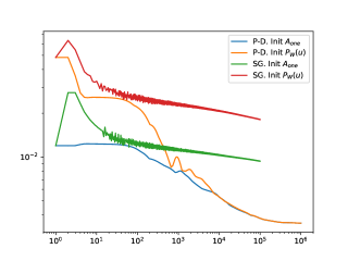
Figure 3.1: Convergence of the objective function for two different optimization algorithms and starting guesses. P.D. = Primal-Dual splitting. S.G.=Subgradient. Here, $m=40$.

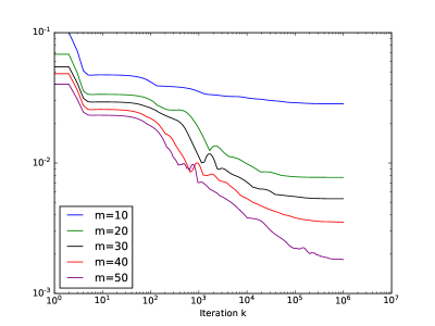
Figure 3.2: Convergence of the objective function in the primal-dual iterations for $m=10,\,20,\,30,\,40,\,50$.

3.3 Numerical tests

We present some numerical experiments, aiming primarily at comparing in terms of the maximum reconstruction error the three above discussed recovery maps: the one-space affine map $A_{n}$, the best affine map $A^{*}_{{\rm msa}}$ for the mean-square error, and the best affine map $A^{*}_{{\rm wca}}$. for the worst case error. In addition, we also consider the mimimum $V$ norm reconstruction map $A(w)=w=P_{W}u$. The results highlight the superiority of the best affine algorithm with respect to the reconstruction error. This comes however at the cost of a computationally intensive training phase as previously described.

We consider the elliptic problem

$$\begin{cases}-{\rm div}\Bigl{(}a(y)\nabla u\Bigr{)}&=f,\quad x\in D\\ \hfill u(x)&=0,\quad x\in\partial D\end{cases}$$ (3.23)

on the unit square $D=]0,1[^{2}$, with a certain parameter dependence in the field $a$. More precisely, for a given $p\geq 1$, we consider “checkerboard” random fields where $a(y)$ is piecewise constant on a $p\times p$ subdivision of the unit-square.

$$D=\bigcup_{i,j=0}^{p-1}S_{i,j},$$

with

$$S_{i,j}:=\Big{[}\frac{i}{p}\,,\frac{i+1}{p}\Big{[}\,\times\,\Big{[}\frac{j}{p}\,,\frac{j+1}{p}\Big{[},\qquad i,j\in 0,\ldots,p-1.$$

The random field is defined as

$$a(y)=1+\frac{1}{2}\sum_{i,j=0}^{p-1}\raise 1.29167pt\hbox{\large$\chi$}_{S_{i,j}}y_{i,j},$$ (3.24)

where $\raise 1.29167pt\hbox{\large$\chi$}_{S}$ denotes the characteristic function of a set $S$, and the $y_{i,j}$ are random coefficients that are independent, each with identical uniform distribution on $[-1,1]$. Thus, our vector of parameters is

$${\bf y}=(y_{i,j})_{i,j=0}^{p-1}\in\mathbb{R}^{p\times p}.$$

In our numerical tests, we take $p=4$, that is $16$ parameters, and work in the ambient space $V=H^{1}_{0}(D)$. All the sets of snapshots used for training and validating the reconstruction algorithms have been computed by first generating a certain number $J$ of random parameters ${\bf y}^{1},\ldots,{\bf y}^{J}$, with each ${\bf y}^{i}\in[-1,1]^{p\times p}$, and then solving the variational form of (3.23) in $V=H^{1}_{0}(D)$ using $\mathbb{P}_{1}$ finite elements on a regular grid of mesh size $h=2^{-7}$. This gives the corresponding solutions $u_{h}^{i}=u_{h}({\bf y}^{i})$ that are used in the computations. To ease the reading, in the following we drop the dependence on $h$ in the notation.

The sensor measurements are modelled with linear functionals that are local averages of the form

$$\ell_{{\bf x},\tau}(u)=\intop\limits_{D}u({\bf r})\varphi_{\tau}({\bf r}-{\bf x})\,\rm{d}{\bf r},$$ (3.25)

where

$$\varphi_{\tau}({\bf r})\propto\mathop{\rm exp}(-|{\bf r}|/2\tau^{2})$$ (3.26)

is a radial function such that $\intop\limits\varphi_{\tau}=1$. The parameter $\tau>0$ represents the spread around the center ${\bf x}$. For the observation space $W$ of our example, we randomly select $m=50$ centers ${\bf x}_{i}\in[0.1,0.9]^{2}$ and spreads $\tau_{i}\in[0.05,0.1]$, and compute the Riesz representers $\omega_{{\bf x}_{i},\tau}$ of $\ell_{{\bf x}_{i},\tau}$ in $H^{1}_{0}(D)$. We then set

$$W\coloneqq\{\omega_{{\bf x}_{i},\tau}\}_{i=1}^{M}$$

which is a space of dimension $m=50$. Figure 3.3 shows the $m$ centers ${\bf x}_{i}$. As an example, the figure also plots the function $\omega_{{\bf x}_{i},\tau}$ for $i=10$, which has center ${\bf x}_{i}=(0.23,0.75)$ and spread $\tau_{i}=0.06$.

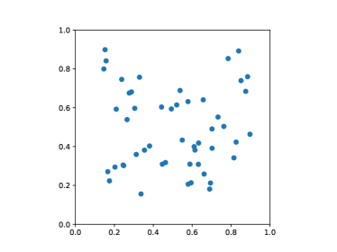
Figure 3.3: Sensor locations and the function $\omega_{{\bf x}_{i},\tau_{i}}$ for $i=10$ (${\bf x}_{i}=(0.23,0.75)$ and $\tau_{i}=0.06$).

As explained in section 3.1, the first step to compute the best algorithm in practice consists in replacing $V=H^{1}_{0}(D)$ by a finite dimensional space that approximates the solution manifold ${\cal M}$ at an accuracy smaller than the one expected for the recovery error. Here, we replace $V$ by $W+V_{N}$ where $V_{N}$ is a reduced basis of dimension $N=110$ that has been generated by running the classical greedy algorithm from [6] over a training set ${\cal M}_{\text{greedy}}$ of $10^{3}$ snapshots. We recall that an idealized version is defined for $n\geq 1$ as

$$u_{n}\in\mathop{\rm argmax}_{u\in{\cal M}_{\text{greedy}}}\|u-P_{V_{n-1}}u\|,\quad V_{n}\coloneqq V_{n-1}\oplus\mathbb{R}u_{n}={\rm span}\{u_{1},\dots,u_{n}\},$$ (3.27)

with the convention $V_{0}\coloneqq\{0\}$. Figure 3.4 gives the decay of the error

$$e_{n}^{\text{(greedy)}}=\max_{u\in{\cal M}_{\text{greedy}}}\|u-P_{V_{n}}u\|$$

across the greedy iterations.

Figure 3.4: Greedy algorithm: decay of the error $e_{n}^{\text{(greedy)}}=\max_{u\in{\cal M}_{\text{greedy}}}||u-P_{V_{n}}u||$.

We next estimate the truncation accuracy $\varepsilon_{N}$ defined in (3.3). This has been done by computing the maximum of the error $\|u-P_{V_{N}}u\|$ over the training set ${\cal M}_{\text{greedy}}$ supplemented by a test set ${\cal M}_{\text{test}}$, also of $10^{3}$ snapshots. We obtain the estimate

$$\max_{u\in{\cal M}_{\text{greedy}}\cup{\cal M}_{\text{test}}}\|u-P_{V_{N}}u\|\leq\varepsilon_{N}=5.10^{-5}.$$

In the comparison of the three different reconstruction algorithms, we want to illustrate the impact of the number of measurements that are used. To do this, we consider the nested subspaces

$$W_{m}=\mathop{\rm span}\{\omega_{{\bf x}_{i},\tau_{i}}\}_{i=1}^{m}\subset W$$

for $m=10,\,20,\,30,\,40,\,50$ so that $W_{50}=W$.

For the computation of the best affine algorithm, we generate a new training set $\widetilde{\cal M}$ of $10^{3}$ snapshots which we project into $W+V_{N}$. This projected set, which we denote by $P_{W+V_{N}}\widetilde{\cal M}$ with a slight abuse of notation, is used to compute

$$\widetilde{A}^{(m)}_{{\rm wca}}(u)=\widetilde{c}^{(m)}+\widetilde{B}^{(m)}P_{W_{m}}u,\quad m=10,\,20,\dots,\,50,$$

by running the primal-dual algorithm of section 3.2. We have added the indices $m$ to stress that the algorithm depends on it.

For the comparison with the three other reconstruction algorithms, we evaluate

$$e_{{\rm wca}}^{(m)}=\max_{u\in{\cal M}_{\text{test}}}||u-\widetilde{A}^{(m)}_{{\rm wca}}(P_{W_{m}}u)||,\quad m=10,\,20,\dots,\,50.$$

We stress on the fact that the three sets ${\cal M}_{\text{greedy}},\ \widetilde{\cal M}$ and ${\cal M}_{\text{test}}$ are different. We compare this value with the performance of a straightforward reconstruction with the minimal $V$-norm recovery map,

$$e_{{\rm mvn}}^{(m)}=\max_{u\in{\cal M}_{\text{test}}}||u-P_{W_{m}}u||,\quad m=10,\,20,\dots,\,50,$$

with the mean square approach,

$$e_{{\rm msa}}^{(m)}=\max_{u\in{\cal M}_{\text{test}}}||u-\widetilde{A}^{(m)}_{{\rm msa}}(P_{W_{m}}u)||,\quad m=10,\,20,\dots,\,50,$$

and with the best one-space affine algorithm,

$$e_{\mathop{\rm one}}^{(m)}=\min_{1\leq n\leq m}e_{\mathop{\rm one}}^{(m,n)},$$

where

$$e_{\mathop{\rm one}}^{(m,n)}=\max_{u\in{\cal M}_{\text{test}}}||u-A^{(m)}_{n}(P_{W_{m}}u)||,\quad m=10,\,20,\dots,\,50.$$ (3.28)

Some remarks on the computation of the one-space algorithm are in order. First of all, we have used the average

$$\bar{u}:=\frac{1}{\#{\cal M}_{\text{greedy}}}\sum_{u\in{\cal M}_{\text{greedy}}}u$$

as our offset. For $m\leq M$ and $n\leq m$ given, the one-space affine algorithm $A^{(m)}_{n}$ is the one involving the spaces $W_{m}$ and $\widetilde{V}_{n}=\bar{u}+V_{n}$, where $V_{n}={\rm span}\{u_{1},\dots,u_{n}\}$. Its performance is given by $e_{\mathop{\rm one}}^{(m,n)}$ in formula (3.28). Figure 5(a) shows $e_{\mathop{\rm one}}^{(m,n)}$ as a function of $n$ and $m$. Note that, for a fixed $m$, the error $e_{\mathop{\rm one}}^{(m,n)}$ reaches a minimal value $e_{\mathop{\rm one}}^{m}=e_{\mathop{\rm one}}^{(m,n^{*})}$ for a certain dimension $n^{*}=n^{*}(m)$ of the reduced model, given by a thick dot in the figure. This behavior is due to the trade-off between the increase of the approximation properties of $\widetilde{V}_{n}$ as $n$ grows and the degradation of the stability of the algorithm, given by the increase of $\mu(\widetilde{V}_{n},W_{m})$ with $n$. For our comparison purpose, we use $A^{(m)}_{\mathop{\rm one}}=A_{n^{*}(m)}^{(m)}$, that is, the best possible one-space algorithm based on the reduced basis spaces.

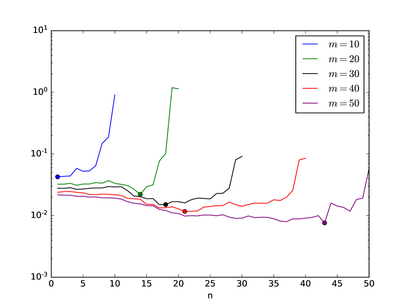
(a) $e_{\mathop{\rm one}}^{(m,n)}$: reconstruction error with $A^{(m)}_{n}$.

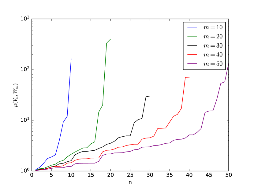
(b) Stability factor $\mu(\widetilde{V}_{n},W_{m})$.

Figure 3.5: one-space algorithm.

Figure 3.6 shows the reconstruction errors $e_{{\rm wca}}^{(m)}$, $e_{{\rm mvn}}^{(m)}$, $e_{{\rm msa}}^{(m)}$ and $e_{\mathop{\rm one}}^{(m)}$ of the four different approaches for $m=10,\,20,\dots,\,50$. We also append a table with the values. We observe that a straightforward reconstruction with the minimal $V$-norm algorithm performs poorly in terms of approximation error and its quality improves only very mildly as we increase the number $m$ of measurements. This justifies considering our three other, more sophisticated, reconstruction algorithms. In this respect, the results confirm first of all that $\widetilde{A}^{(m)}_{{\rm wca}}$ is the best reconstruction algorithm. The mean square approach appears to be slightly superior to the one-space algorithm but still worse than the best affine algorithm. Note that the accuracy improvement between the best affine algorithm and the one-space and mean square algorithms is of about a half order of magnitude for each $m$.

Last but not least, we give some illustrations on the reconstruction algorithms applied to a particular snapshot function $u$ from the test set ${\cal M}_{\text{test}}$. The target function is given in Figure 3.7 and Figures 3.8 and 3.9 show the resulting reconstructions of $u$ from $P_{W_{m}}u$ with our four different algorithms and for $m=20$ and $40$. Visually, the reconstructed functions look very similar. However, the difference in quality can be better appreciated in the plots of the spatial errors $|u({\bf x})-A^{(m)}(u)({\bf x})|$ as well as in the derivatives and their corresponding spatial errors.

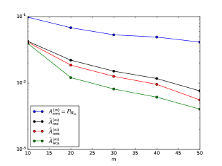
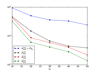
Figure 3.6: Comparison of the reconstruction errors (left: $H^{1}_{0}(D)$ norm; right: $L^{2}(D)$ norm).

Figure 3.7: Function $u$ (left) and $\partial u/\partial x$ (right). The reconstruction of this function is given in Figures 3.8 and 3.9.

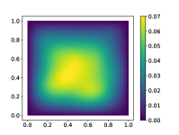
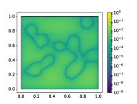
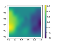
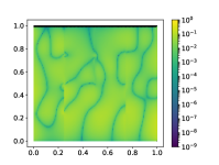
(a) Minimal $V$-norm: $P_{W_{20}}(u)$.

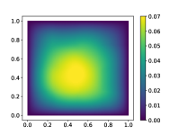
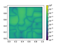
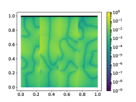
(b) one-space affine: $A^{(20)}_{\mathop{\rm one}}\Bigl{(}P_{W_{20}}(u)\Bigr{)}$

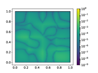
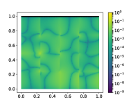
(c) Mean Square Algorithm: $\widetilde{A}^{(20)}_{{\rm msa}}\Bigl{(}P_{W_{20}}(u)\Bigr{)}$

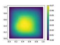
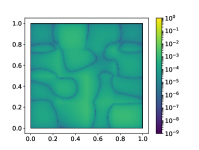
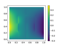
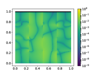
(d) Best affine: $\widetilde{A}^{(20)}_{{\rm wca}}\Bigl{(}P_{W_{20}}(u)\Bigr{)}$

Figure 3.8: Reconstruction of the given function $u$ $(m=20)$. For each reconstruction strategy: (i) the two first figures are $A^{(m)}(u)({\bf x})$ and the spatial errors $|u({\bf x})-A^{(m)}(u)({\bf x})|$, (ii) the two last figures are $\frac{\partial A^{(m)}(u)}{\partial x}({\bf x})$ and the spatial errors $|\frac{\partial u}{\partial x}({\bf x})-\frac{\partial A^{(m)}(u)}{\partial x}({\bf x})|$.

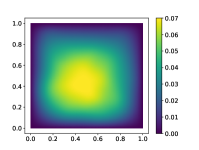
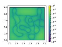
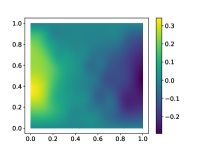
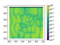
(a) Minimal $V$-norm: $P_{W_{40}}(u)$.

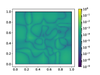
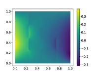
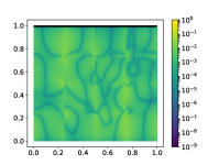
(b) one-space affine: $A^{(40)}_{\mathop{\rm one}}\Bigl{(}P_{W_{40}}(u)\Bigr{)}$

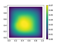
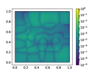
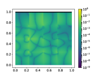
(c) Mean Square Algorithm: $\widetilde{A}^{(40)}_{{\rm msa}}\Bigl{(}P_{W_{40}}(u)\Bigr{)}$

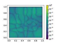
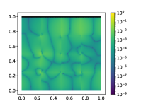
(d) Best affine: $\widetilde{A}^{(40)}_{{\rm wca}}\Bigl{(}P_{W_{40}}(u)\Bigr{)}$

Figure 3.9: Reconstruction of the given function $u$ $(m=40)$. For each reconstruction strategy: (i) the two first figures are $A^{(m)}(u)({\bf x})$ and the spatial errors $|u({\bf x})-A^{(m)}(u)({\bf x})|$, (ii) the two last figures are $\frac{\partial A^{(m)}(u)}{\partial x}({\bf x})$ and the spatial errors $|\frac{\partial u}{\partial x}({\bf x})-\frac{\partial A^{(m)}(u)}{\partial x}({\bf x})|$.

Let us briefly discuss the complexity of the primal-dual algorithm. At each iteration of the algorithm, the main bottleneck is the computation of $L^{*}$ (equation (3.21)). It requires to do $J$ matrix-vector products with the matrices $Q_{j}\in\mathbb{R}^{N\times m(N+1)}$ and then do a summation of the resulting vectors. The cost of these operations thus increases linearly with $J$ in terms of computational time and memory ressources. In fact, the limitation in memory was the main reason to fix $J=10^{3}$ and not work with a larger number of training snapshots. Let us make a quick count on the cost in terms of the number of elements to store at each iteration. The matrices $Q_{j}$ are sparse. For each row, there are $m+1$ nonnegative coefficients. Therefore we need to store $N(m+1)$ coefficients for each matrix, therefore a total number of $JN(m+1)$ coefficients. In our case, $N=110$ was carefully fixed to guarantee that

$$\max_{u\in{\cal M}_{\text{greedy}}\cup{\cal M}_{\text{test}}}\|u-P_{V_{N}}u\|\leq\varepsilon_{N}=5.10^{-5}.$$

We have $m$ ranging between $10$ and $50$. Thus the number of nonnegative elements that we have to store for each $Q_{j}$ ranges between $1210$ and $5610$. Therefore, taking $J=10^{3}$ as in our computation, we need to handle a total number of coefficients ranging between $1.21.10^{6}$ and $5.61.10^{6}$.

4 Conclusions

In this paper, we have studied the notion of a best affine recovery map for a general state estimation problem, that is, the map $A^{*}_{\rm wca}$ that minimizes the worst case error $E_{{\rm wc}}(A,{\cal M})$ among all affine maps. This map is the solution to a convex optimization problem. Up to the additional perturbation induced from replacing ${\cal M}$ by a discrete training set $\widetilde{\cal M}$, it can be efficiently computed by a primal-dual optimization algorithm. Since any affine recovery map is associated with a reduced basis $V_{n}$ plus an offset $\bar{u}$, the optimal affine map amounts to applying the one-space method from [19] using an affine reduced model space $\bar{u}+V_{n}$ which is optimal for the reconstruction task. Our numerical tests confirm that this choice outperforms standard reduced basis spaces, which are not specifically constructed for the recovery problem, but rather for the approximation of ${\cal M}$.

Our approach is readily applicable to any type of parametric PDEs, ranging from linear PDEs with affine parameter dependence to non-linear PDEs with non-affine parameter dependence. We outline its main limitations:

• The first essential limitation lies in its confinement to linear or affine recovery algorithms. Let us stress that state estimation is a linear inverse problem in the sense that the observed data $w$ is generated from $u$ by a linear projection, optimal recovery among all possible maps, due to the complex nonlinear geometry of the solution manifold ${\cal M}$ that constitutes the prior. Therefore, going beyond the results provided by our method requires the development of nonlinear recovery strategies. One possible approach, currently under investigation, is to (i) consider a collection affine reduced model spaces $\{\bar{u}_{k}+V^{k}\,:\,k=1,\dots K\}$, each of them of dimension $n_{k}\leq m$, (ii) use the observed data $w$ to properly select a particular space from this collection and (iii) apply the affine recovery algorithm using this particular data-dependent space. One standard way to obtain such local reduced model spaces is by splitting the parameter domain and searching for local reduced bases or POD, as for example proposed in [1] for forward modeling or in [14] for state estimation. However, the optimal affine recovery approach discussed in the present paper could also be used in order to improve on such constructions.

• The developed approach implicitly assumes that the parametric PDE model is perfect although, in full generality, the true physical state may not belong to ${\cal M}$. It is also assumed that measurements are noiseless. One way to readily extend this approach to the search of optimal affine maps that take into account model bias and measurement noise is as follows: suppose that the model bias is of size $\delta>0$ in the sense that the real physical state $u$ belongs to the offset

  $${\cal M}_{\delta}:=\{v\in V\,:\,\exists y\in Y\text{ s.t. }\|v-u(y)\|\leq\delta\}.$$

  Suppose further that measurements are given with some deterministic noise, that is, we are given $P_{W}u+\eta$ such that $\|\eta\|\leq\sigma$ for some noise level $\sigma$. Then, the optimal affine map is given by

  $$\min_{A\text{ affine}}\;\max_{\begin{subarray}{c}u\in{\cal M}_{\delta},\\ \|\eta\|\leq\sigma\end{subarray}}\|u-A(P_{W}u+\eta)\|$$

  Once again we may emulate this optimization by introducing a discrete training set. Let us stress that such an optimization problem requires the knowledge of the size of the model bias $\delta$ and the noise level $\sigma$. While $\sigma$ may be known for some applications, $\delta$ is very hard to estimate in practice.

An assessment of the obtained estimation accuracy relies, however, on the availability of computable bounds for the distance of the reduced spaces from the solution manifold which may depend on the type of the PDE model.

References

- [1] D. Amsallem, C. Farhat and M.J. Zahr, Nonlinear model order reduction based on local reduced order bases, International Journal for Numerical Methods in Engineering 92, 891-916, 2012.
- [2] P. Binev, A. Cohen, W. Dahmen, R. DeVore, G. Petrova, and P. Wojtaszczyk, Convergence Rates for Greedy Algorithms in Reduced Basis Methods, SIAM Journal of Mathematical Analysis 43, 1457-1472, 2011.
- [3] P. Binev, A. Cohen, W. Dahmen, R. DeVore, G. Petrova, and P. Wojtaszczyk, Data assimilation in reduced modeling, SIAM Journal on Uncertainty Quantification, 5, 1–29, 2017.
- [4] P. Binev, A. Cohen, O. Mula and J. Nichols, Greedy algorithms for optimal measurements selection in state estimation using reduced models, SIAM Journal on Uncertainty Quantification 43, 1101-1126, 2018.
- [5] B. Bojanov, Optimal recovery of functions and integrals. First European Congress of Mathematics, Vol. I (Paris, 1992), 371-390, Progr. Math., 119, Birkhauser, Basel, 1994.
- [6] A. Buffa, Y. Maday, A.T. Patera, C. Prud’homme, and G. Turinici, A Priori convergence of the greedy algorithm for the parameterized reduced basis, ESAIM M2AN 46, 595-603, 2012.
- [7] A. Chambolle and T. Pock, A first-order primal-dual algorithm for convex problems with applications to imaging, Journal of Mathematical Imaging and Vision, 40, 120-145, 2011.
- [8] A. Cohen, W. Dahmen and R. DeVore, Reduced basis greedy selection using random training sets, submitted, 2018.
- [9] A. Cohen and R. DeVore, Approximation of high dimensional parametric pdes, Acta Numerica 24, 1-159, 2015.
- [10] A. Cohen, R. DeVore and C. Schwab, Analytic Regularity and Polynomial Approximation of Parametric Stochastic Elliptic PDEs, Analysis and Applications 9, 11-47, 2011.
- [11] R. DeVore, G. Petrova, and P. Wojtaszczyk, Greedy algorithms for reduced bases in Banach spaces, Constructive Approximation, 37, 455-466, 2013.
- [12] M. Dashti and A.M. Stuart, The Bayesian Approach to Inverse Problems, Handbook of Uncertainty Quantification, Editors R. Ghanem, D. Higdon and H. Owhadi, Springer, 2015.
- [13] J. Fadili and O. Mula, Primal-dual splitting for the max of convex functions, in progress.
- [14] F. Galarce, J.-F. Gerbeau, D. Lombardi and O. Mula, State estimation with nonlinear reduced models - Application to the reconstruction of blood flows with doppler ultrasound images, submitted 2019.
- [15] P.L.Houtekamer, H.L. Mitchell, Ensemble Kalman filtering, Q. J. R. Meteorol. Soc. 131, 3269–3289, 2005.
- [16] M. Kärcher, S. Boyaval, M.A. Grepl and K. Veroy, Reduced basis approximation and a-posteriori error bounds for 4D-Var data assimilation, J. Optimization and Engineering 19, 663-695, 2018.
- [17] K. Law, A. Stuart, and K. Zygalakis, Data Assimilation, A Mathematical Introduction, Text in Applied Mathematics, Springer-Verlag, 2015.
- [18] A.C. Lorenc, A global three-dimensional multivariate statistical interpolation scheme, Monthly Weather Review 109, 701-721, 1981.
- [19] Y. Maday, A.T. Patera, J.D. Penn and M. Yano, A parametrized-background data-weak approach to variational data assimilation: Formulation, analysis, and application to acoustics, Int. J. Numer. Meth. Eng.102, 933-965, 2015.
- [20] C.A. Micchelli, T.J. Rivlin, Lectures on optimal recovery. Numerical analysis, Lancaster 1984 (Lancaster, 1984), 21-93, Lecture Notes in Math., 1129, Springer, Berlin, 1985.
- [21] E. Novak and H. Wozniakowski, Tractability of Multivariate Problems, Volume I: Linear Information, EMS Tracts in Mathematics, Vol. 6 Eur. Math. Soc. Publ. House, Zurich 2008
- [22] G. Rozza, D.B.P. Huynh, and A.T. Patera, Reduced basis approximation and a posteriori error estimation for affinely parametrized elliptic coercive partial differential equations Ñ application to transport and continuum mechanics, Archive of Computational Methods in Engineering 15, 229–275, 2008.
- [23] S. Sen, Reduced-basis approximation and a posteriori error estimation for many-parameter heat conduction problems, Numerical Heat Transfer B-Fund 54, 369–389, 2008.
- [24] A. M. Stuart, Inverse problems: A Bayesian perspective, Acta Numerica 19, 451-559, 2010.
- [25] T. Taddei, An adaptive parametrized-background data-weak approach to variational data assimilation, ESAIM M2AN 51, 1827-1858, 2017.
- [26] B. Peherstorfer, K. Willcox, M. Gunzburger, Survey of multifidelity methods in uncertainty propagation, inference, and optimization, SIAM Review, Vol. 60, No. 3, pp. 550–591, 2018.