The Hall effect in ballistic flow of two-dimensional interacting particles

Abstract

In high-quality solid-state systems at low temperatures, the hydrodynamic or the ballistic regimes of heat and charge transport are realized in the electron and the phonon systems. In these regimes, the thermal and the electric conductance of the sample can reach abnormally large magnitudes. In this paper, we study the Hall effect in a system of interacting two-dimensional charged particles in a ballistic regime. We demonstrated that the Hall electric field is caused by a change in the densities of particles due to the effect of external fields on their free motions between the sample edges. In one-component (electron or hole) systems the Hall coefficient turns out to one half compared with the one in conventional disordered Ohmic samples. This result is consistent with the recent experiment on measuring of the Hall resistance in ultra-high-mobility GaAs quantum wells. In two-component electron-hole systems the Hall electric field depends linearly on the difference between the concentrations of electrons and holes near the charge neutrality point (the equilibrium electron and hole densities coincide) and saturates to the Hall field of a one-component system far from the charge neutrality point. We also studied the corrections to magnetoresistance and the Hall electric field due to inter-particle scattering being a precursor of forming a viscous flow. For the samples shorter than the inter-particle scattering length, the obtained corrections govern the dependencies of magnetoresistance and the Hall field on temperature.

I Introduction

In novel high-quality nanostructures and bulk materials extremely small densities of defects can be achieved. At low temperatures the electron mean free paths relative to scattering on disorder and on phonons in such material become very long. In this connection, the hydrodynamic and the ballistic regimes of transport can be realized in mesoscopic or even macroscopic samples. In 1960-1970s the theory of the hydrodynamic regime of electron heat and charge transport was developed for bulk metals by R. N. Gurzhi and coauthors Gurzhi_rev . The ballistic electron transport of 2D electrons in semiconductor quantum wells was extensively studied theoretically and experimentally in 1980-1990s in several groups rev_bal . In recent decade the bright evidences of realization of the hydrodynamic and the ballistic regimes of transport were discovered in several novel materials: high-mobility GaAs quantum wells, single-layer graphene, 3D Weyl semimetals exp_hydgr_1 ; exp_hydgr_1_2 ; exp_hydgr_1_3 ; exp_hydgr_1_4 ; exp_hydgr_1_ov ; exp_hydgr_2 ; exp_hydgr_3 ; exp_hydgr_4 ; exp_hydgr_4_2 ; gr_neg_MR ; Gusev_1 ; Gusev_2 ; Gusev_3 ; exp_gr_1 ; exp_gr_2 ; exp_gr_3 ; exp_gr_4 . Theory of hydrodynamic and ballistic transport in solids has been developed in the last years in many different directions: both aimed for explaining recent experiments as well as in areas not directly related to recent experiments hydr_tr_th_2 ; hydr_tr_th_3 ; hydr_tr_th_4 ; hydr_tr_th_5 ; hydr_tr_th_6 ; hydr_tr_th_7 ; hydr_tr_th_8 ; hydr_tr_th_9 ; hydr_tr_th_10 ; hydr_tr_th_10_2 ; hydr_tr_th_11 ; hydr_tr_th_11_2 ; hydr_tr_th_11_3 ; hydr_tr_th_12 ; we_hd ; we_hd_2 ; we_hd_3 ; we_hd_4 ; we_hd_5 ; we_hd_5_2 ; th_therm_gr_hydr_1 ; th_therm_gr_hydr_2 ; paper_mail ; paper_rec_1 ; Hall_visc ; ours_bal ; Kiselev ; recentest ; recentest2 ; recentest3 ; new ; new_2 .

The giant negative magnetoresistance effect is considered to be one of the main evidences of realization of the hydrodynamic regime of charge transport. It was observed in high-mobility GaAs quantum wells, in the 3D Weyl semimetal WP₂, and, very recently, in single-layer graphene exp_hydgr_1 ; exp_hydgr_1_2 ; exp_hydgr_1_3 ; exp_hydgr_1_4 ; exp_hydgr_1_ov ; exp_hydgr_2 ; exp_hydgr_3 ; gr_neg_MR ; Gusev_1 . The giant negative magnetoresistance often consists of a temperature-dependent wide peak with a large amplitude and of a temperature-independent small narrow peak. The temperature-dependent part of the giant negative magnetoresistance was explained as the result of forming the viscous electron fluid and the magnetic field dependence of the electron viscosity hydr_tr_th_9 . An explanation of the temperature-independent part was proposed in Ref. ours_bal within the model of ballistic transport of 2D interacting electrons. In was noted in Ref. ours_bal that a small external magnetic field leads to the increase of the average free path of ballistic electrons in a long sample. This fact results in a small negative magnetoresistance, which can be temperature-independent for not very long samples, where the maximum length of ballistic trajectories is restricted by the sample size.

For identification of the ballistic and the hydrodynamic regimes of electron transport, are important not only measurements of magnetoresistance and the size dependencies of resistance in zero magnetic field. Studies of the Hall effect are also of great importance gr_neg_MR ; Gusev_3 ; Hall_visc ; new ; new_2 . In Refs. gr_neg_MR ; Gusev_3 the Hall resistance in best-quality graphene and ultra-high mobility GaAs quantum wells was measured at the conditions when the hydrodynamic and the ballistic regime were apparently realized. Substantial deviations of the Hall resistance from its usual value for a long Ohmic disordered sample were observed. In Ref. Hall_visc the crossover between the hydrodynamic and the ballistic regimes of transport, in particular, evolution of the longitudinal and the Hall resistances, were studied for 2D electrons in a long sample by numerical solution of the kinetic equation. However, in that work the specific mechanisms of the Hall effect in the ballistic regime and the role of the electron-electron scattering in this regime were not clarified.

In Refs. new ; new_2 the Hall effect was theoretically studied for a system of a 2D interacting electrons in a weak disorder. The main attention was paid to the regime of moderate magnetic field corresponding to the cyclotron radius of the order of the sample width. It was demonstrated that the curvature of the Hall electric field in the center of the sample can be used to distinguish the Ohmic, ballistic and hydrodynamic regimes new . In Ref. new_2 a method of experimental measurements of a generalized Hall viscosity were proposed at the crossover between the ballistic and the hydrodynamic regime of transport in the Hall and Corbino samples.

In this paper we develop a theory of the Hall effect in one-component and two-component conduction systems of interacting particles in ballistic samples at small magnetic fields rep . We study the Hall effect for low magnetic field when the magnetic field term in the kinetic equation can be treated as a perturbation. Due to the kinematic effect of the external fields on the ballistic trajectories, the electron and hole densities become inhomogeneous and not equal one to another that leads to arising the Hall electric field. The resulting Hall coefficient turns out to be one half of the Hall coefficient $R_{H}^{0}$ of the conventional Ohmic bulk conductor at zero temperature. We demonstrate that the obtained result is consistent with the experimental data Gusev_3 .

For two-component electron-hole systems, we studied the Hall effect in the simplest case of a structure with a metallic gate and at high temperature. The Hall electric field is strongly suppressed as compared with the case of one-component systems if the equilibrium electron and hole densities are close to each other and rapidly saturates to the result for a one-component system if the equilibrium electron and hole densities becomes substantially different.

We also studied the hydrodynamic corrections to the Hall effect and magnetoresistance in the ballistic regime, resulted from the arrival terms of the inter-particle collisions integrals. The hydrodynamic corrections, being a precursor of formation a viscous flow, arise due to electron-electron and hole-hole collisions conserving momentum and protecting a particle from the loss of its momentum at scattering on the sample edges.

II One-component systems

II.1 Model

We consider a flow of 2D charged particles (electrons or holes) in a long sample with the width $W$ and the length $L\gg W$ [see Fig. 1(a)]. We seek a linear response on a homogeneous generalized external field ${\bm{E}}_{0}||x$ in the presence of a magnetic field ${\bm{B}}$ perpendicular to the sample plane. The amplitude of the field $E_{0}$ is proportional to a gradient of temperature for the problem of heat transport and coincides with an external electric field for the problem of charge transport. If the mean free path relative to the inter-particle collisions, $l$, is much larger than the sample width $W$, $l\gg W$, the collisions with the longitudinal sample edges are the most frequent type of scattering events and the ballistic regime of heat or charged transport is realized.

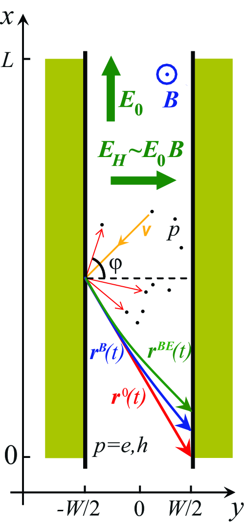
Figure 1: A schematic illustration of a ballistic sample with particles $p$ and rough edges in external electric and magnetic fields $E_{0}$ and $B$.

In the current study we consider the sample to be enough clean and thus neglect particle scattering on disorder. We assume the particle dispersion law to be quadratic.

The linear response of particles to the external field $E_{0}$ is described by the inequilibrium part of the distribution function

$$\delta f(y,\mathbf{p})=-f_{F}^{\prime}(\varepsilon)f(y,\varphi,\varepsilon)\sim E_{0}\>,$$ (1)

where $f_{F}(\varepsilon)$ is the Fermi distribution function, $\varepsilon$ is the particle energy, $\varphi$ is the angle of the particle velocity $\mathbf{v}=v(\varepsilon)[\,\cos\varphi,\,\sin\varphi\,]$, $\mathbf{p}=m\mathbf{v}$ is the particle momentum, and $m$ is the particle mass. see Fig. 1. The dependence of $\delta f$ on the coordinate $x$ is absent due to the relation $L\gg W$.

For simplicity, we use the rough approximation in which the energy dependencies in the absolute value of the particle velocity $v(\varepsilon)$ and in the factor $f(y,\varphi,\varepsilon)$ of the inequilibrium part of distribution function $\delta f(y,\mathbf{p})$ are omitted.

We use the system of units in which the characteristic particle velocity $v(\varepsilon)\equiv v$ is equal to unity and coordinates, time, and the reciprocal force from the generalized external field, $1/(eE_{0})$, are measured in the same units. Here we introduce the dimensionless particle charge $e=\pm 1$ in the expression for the external force $eE_{0}$ in order to be able to specify the sign of the charge of particles for the problem of electric transport.

The kinetic equation for the truncated distribution function $f(y,\varphi)$ takes the form (see Ref. ours_bal and Fig. 1):

$$\cos\varphi\,\frac{\partial f}{\partial y}-\sin\varphi\,eE_{0}-\cos\varphi\,eE_{H}+\omega_{c}\,\frac{\partial f}{\partial\varphi}=\mathrm{St}[f]\>,$$ (2)

where the collision integral $\mathrm{St}$ describes the inter-particle scattering conserving momentum, $\omega_{c}\sim eB$ is the cyclotron frequency, and $E_{H}$ is the Hall electric field arising due to the presence of the magnetic field and related to redistribution of the 2D charged particles. In Eq. (2) we neglect scattering processes which do not conserve momentum. Following Ref. book__gas__the_method and Refs. hydr_tr_th_10 ; hydr_tr_th_10_2 ; hydr_tr_th_11 ; hydr_tr_th_11_2 ; hydr_tr_th_11_3 , we use the simplified form of the collision integral $\mathrm{St}$ :

$$\begin{array}[]{c}\displaystyle\mathrm{St}[f]=-\gamma\,(f-P[f])\>,\end{array}$$ (3)

where $\gamma$ is the scattering rate, while $P$ is the projector of distribution function $f(\varphi)$ on the subspaces consisting of the basis functions $\{1,e^{\pm i\varphi}\}$. The operator $\mathrm{St}$ conserves the perturbations of the distribution function corresponding to a nonzero homogeneous flow and to a non-equilibrium concentration.

We assume the longitudinal sample edges being rough and the scattering of particles on them being fully diffusive. Thus the boundary conditions on the distribution function are as follows: $f(-W/2,\varphi)=c_{l}$ on the interval $-\pi/2<\varphi<\pi/2$ at the left sample edge, $y=-W/2$ (see Fig. 1), and $f(W/2,\varphi)=c_{r}$ on the interval $\pi/2<\varphi<3\pi/2$ at the right edge. Here the quantities $c_{l}$ and $c_{r}$ are the values of the distribution function $f$ averaged over the angles of the particles trajectories reflected from the edges $y=\mp W/2$ rev_bal :

$$\begin{array}[]{c}\displaystyle c_{l}=-\frac{1}{2}\int_{\pi/2}^{3\pi/2}d\varphi^{\prime}\>f(-W/2,\varphi^{\prime})\cos\varphi^{\prime}\>,\\ \\ \displaystyle c_{r}=\frac{1}{2}\int_{-\pi/2}^{\pi/2}d\varphi^{\prime}\>f(W/2,\varphi^{\prime})\cos\varphi^{\prime}\>.\end{array}$$ (4)

Such boundary conditions just express the fact that the $y$ component of the particle flow $j_{y}(y)$ vanishes at the edges (and thus everywhere in the sample due to the continuity equation $\mathrm{div}\,\mathbf{j}=0$).

The kinetic equation (2) can be rewritten as:

$$\Big{[}\cos\varphi\,\frac{\partial}{\partial y}+\gamma\Big{]}\widetilde{f}-\sin\varphi\,eE_{0}=\gamma P[\widetilde{f}\,]-\omega_{c}\,\frac{\partial\widetilde{f}}{\partial\varphi}\>,$$ (5)

where we introduced the function

$$\widetilde{f}(y,\varphi)=f(y,\varphi)+e\phi(y)\>,$$ (6)

in which $\phi$ is the electrostatic potential of the Hall electric field: $E_{H}=-\phi^{\prime}$.

In Ref. ours_bal we analyzed this kinetic equation in limiting regimes $\gamma W\gg 1$ and $\gamma W\ll 1$ for the case of zero magnetic field, $\omega_{c}=0$. We demonstrated that in the hydrodynamic regime, $\gamma W\gg 1$, the left and the right parts of Eq. (5) are of the same order of magnitude and Eq. (5) transforms into the Navier-Stocks equation for the density of the particle (or heat) flow $j(y)\equiv j_{x}(y)$:

$$j(y)=\frac{n_{0}}{\pi m}\int_{0}^{2\pi}d\varphi\>\sin\varphi\,f(y,\varphi)\>,$$ (7)

while in the ballistic regime, $\gamma W\ll 1$, each term in the left part of (5) is much larger than the right part term $\gamma P[\widetilde{f}]$. In Eq. (7) $n_{0}$ is the equilibrium density of particles (or particle energy) and $m$ is the particle mass. Note that the exact form of Eq. (7) is due to the quadratic energy spectrum of the particles.

For the case of the a nonzero magnetic field, one can again prove that the arrival term $\gamma P[\widetilde{f}\,]$ in the ballistic regime, $\gamma W\ll 1$, can be treated as a perturbation if the magnetic field is enough small [the term $\omega_{c}\,\partial\widetilde{f}/\partial\varphi$ is smaller than all other terms in the left part of Eq. (5)]. In particular, this is the true for the first-order by $\omega_{c}$ contribution to the particle distribution function $f_{1}\sim\omega_{c}$, which describes the Hall effect.

For brevity, further we will omit the tilde in designation of $\widetilde{f}$ and just imply $f\equiv\widetilde{f}$.

II.2 Transport in zero magnetic field

The solution of the kinetic equation (5) with the zero right part and the boundary conditions (4) has the form ours_bal : $f(y,\varphi)=f_{+}(y,\varphi)$ at $-\pi/2<\varphi<\pi/2$ and $f(y,\varphi)=f_{-}(y,\varphi)$ at $\pi/2<\varphi<3\pi/2$, where

$$f_{\pm}(y,\varphi)=eE_{0}\,\frac{\sin\varphi}{\gamma}\Big{[}1-\exp\Big{(}\displaystyle-\gamma\,\frac{y\pm W/2}{\cos\varphi}\Big{)}\Big{]}\>.$$ (8)

For a long sample, $L\gg 1/\gamma$, the flow density corresponding to Eq. (8) at $\gamma W\ll 1$ in the main order by the logarithm $\ln\left[1/(\gamma W\right)]$ is homogeneous:

$$j(y)=j_{0}=\frac{2en_{0}E_{0}W}{\pi m}\ln\Big{(}\frac{1}{\gamma W}\Big{)}\>.$$ (9)

For the total electric current

$$I_{0}=e\int_{-W/2}^{W/2}dy\,j(y)$$ (10)

we obtain:

$$I_{0}=\frac{2e^{2}n_{0}E_{0}W^{2}}{\pi m}\ln\Big{(}\frac{1}{\gamma W}\Big{)}\>.$$ (11)

It is seen from Eq. (8) that the logarithmic divergence in $j_{0}$ is related to the particles with the velocity angles $\varphi$ in the diapason $||\varphi|-\pi/2|\lesssim\delta_{m}$, where $\delta_{m}=\gamma W\ll 1$ is the characteristic value of the difference $|\pi/2-|\varphi||$ corresponding to the particles giving the main contribution to the current. Such particles are moving almost parallel to the sample direction. A particle on such “special” trajectories spends a longer time between scattering events on the opposite edges as compared to the particles moving along the “regular” trajectories with $\varphi\sim 1$ and, thus, acquires a larger velocity correction due to acceleration by the field $E_{0}$.

A more exact solution of Eq. (5) with taking into account the arrival term in the collision integral, $\gamma P[f]$, provides a hydrodynamic correction $\delta I_{h}$ to the current $I_{0}$ ours_bal . Such correction is related to the inter-particle collisions conserving momentum, which protect particles from a loss of their momentum in scattering on edges. In order to calculate the hydrodynamic correction in the ballistic limit, $\gamma W\ll 1$, we present the distribution function in the form $f=f_{0}+f_{1}$, where $f_{0}$ is the function (8) and $f_{1}$ is a correction to $f_{0}$ corresponding to the non-zero right part of Eq. (5), $\gamma P[f]$. The equation for $f_{1}$ takes the form:

$$\Big{[}\cos\varphi\,\frac{\partial}{\partial y}+\gamma\Big{]}f_{1}=\gamma P_{\sin}[f_{0}]\>,$$ (12)

where $P_{\sin}$ is the projector on the function $\sin\varphi$.

Action of the operator $P_{\sin}$ on the zero-order distribution function $f_{0}$ yields a value proportional to the current density: $P_{\sin}[f_{0}]=j(y)\sin\varphi/(n_{0}/m)$, where $j(y)=j_{0}$ is given by Eq. (9). Therefore, the right part of Eq. (12) becomes equal just to $qE_{0}\sin\varphi$, where

$$q=\frac{2}{\pi}\,\gamma W\,\ln\Big{(}\frac{1}{\gamma W}\Big{)}\ll 1\>.$$ (13)

By this way, Eq. (12) turns into Eq. (5) with zero right part and the value $E_{0}$ replaced by $qE_{0}$. Thus for all the values related to the first hydrodynamic correction $f_{1}$ we just have in the main order by the logarithm $\ln[1/(\gamma W)]$: $f_{1}(y,\varphi)=qf_{0}(y,\varphi)$, $j_{1}(y)=qj_{0}(y)$, and $I_{1}\equiv\delta I_{h}=qI_{0}$, namely:

$$\delta I_{h}=\frac{4e^{2}n_{0}E_{0}\gamma W^{3}}{\pi^{2}m}\ln\Big{(}\frac{1}{\gamma W}\Big{)}^{2}\>.$$ (14)

The obtained correction (14) is positive and originates from the small group of particles whose last scattering event was an inter-particle collision. By this way, arising of the correction $\delta I_{h}$ due to such particles is a precursor of forming the Poiseuille flow of a viscous fluid related to the inter-particle collisions conserving momentum.

II.3 Magnetotransport

II.3.1 The Hall effect

In this subsection we study the Hall effect and magnetoresistance of the one-component system in the ballistic regime, $\gamma W\ll 1$, within the kinetic equation (5).

As it was discussed above, at enough small $\omega_{c}$ the arrival term $\gamma P[f]$ in the main order by the logarithm $\ln[1/(\gamma W)]\gg 1$ can be neglected in the main approximation by $\gamma$ and the kinetic equation (5) takes the form:

$$\left[\cos\varphi\,\frac{\partial}{\partial y}+\gamma\right]f+\sin\varphi\,eE_{0}=-\omega_{c}\frac{\partial f}{\partial\varphi}\>.$$ (15)

The right part of this equation is a small perturbation as compared to the left part.

We seek the solution of Eq. (15) in the form of the series $f=f_{0}+f_{1}+f_{2}$, where $f_{0}$ is given by Eq. (8), while $f_{1}$ and $f_{2}$ are proportional to the powers of magnetic field: $f_{1}\sim\omega_{c}\sim B$, $f_{2}\sim\omega_{c}^{2}\sim B^{2}$. For the functions $f_{1}$ and $f_{2}$ we obtain from Eq. (15):

$$\Big{[}\cos\varphi\frac{\partial}{\partial y}+\gamma\Big{]}f_{1}=-\omega_{c}\frac{\partial f_{0}}{\partial\varphi}\>,$$ (16)

$$\Big{[}\cos\varphi\frac{\partial}{\partial y}+\gamma\Big{]}f_{2}=-\omega_{c}\frac{\partial f_{1}}{\partial\varphi}\>.$$ (17)

The solution of Eq. (16) for the zero boundary conditions with $c_{l,r}\equiv 0$ in Eqs. (4) is

$$\begin{array}[]{c}\displaystyle f_{1}^{z}(y,\varphi)=-\omega_{c}eE_{0}\Big{\{}\frac{\cos\varphi}{\gamma^{2}}-\exp\Big{[}-\gamma\,\frac{y\pm W/2}{\cos\varphi}\Big{]}\\ \\ \displaystyle\times\Big{[}\frac{\cos\varphi}{\gamma^{2}}+\frac{y\pm W/2}{\gamma}-\frac{\sin^{2}\varphi}{2\cos^{3}\varphi}\,\Big{(}y\pm\frac{W}{2}\,\Big{)}^{2}\,\Big{]}\,\Big{\}},\end{array}$$ (18)

where the signs $\pm$ corresponds to the diapasons of the angles $-\pi/2<\varphi<\pi/2$ and $\pi/2<\varphi<3\pi/2$, respectively. It can be seen from comparison of Eqs. (8) and (18) that the perturbation theory by the magnetic field term can be used in low magnetic field until

$$\omega_{c}\ll\gamma^{2}W\>.$$ (19)

The function $f_{1}$ satisfying the non-zero boundary conditions with $c_{l,r}$ from Eqs. (4) has the form: $f_{1}=f_{1}^{z}+\delta f_{1}$, where

$$\delta f_{1}(y,\varphi)=C_{\pm}\exp\Big{(}-\gamma\frac{y\pm W/2}{\cos\varphi}\Big{)}$$ (20)

is some solution of Eq. (16) with the zero right part. A straightforward calculations based on (18) lead to the proper values of the coefficients $C_{\pm}$:

$$C_{\pm}=\pm\omega_{c}eE_{0}\frac{W}{4\gamma}\>.$$ (21)

The resulting correction $\delta f_{1}$ is much smaller than $f_{1}^{z}$ at the angles $||\varphi|-\pi/2|\lesssim\delta_{m}$.

If a current flows through a sample in magnetic field, a perturbation of the charged particle density and the Hall electric field arises due to the magnetic Lorentz force. In our system these effects are described by the zero angular harmonic of the function $f_{1}$

$$f^{m=0}_{1}(y)=\frac{1}{2\pi}\int_{0}^{2\pi}d\varphi\>f_{1}(y,\varphi)\>.$$ (22)

From Eqs. (18), (20), (21), and (22) in the main order by $1/(\gamma W)$ and $\ln[1/(\gamma W)]$ we obtain:

$$f_{1}^{m=0}(y)=-\frac{\omega_{c}eE_{0}}{\pi}\,Wy\,\ln\Big{(}\frac{1}{\gamma W}\Big{)}$$ (23)

The other terms in decomposition of $f_{1}^{m=0}$ by the parameter $\gamma W$ are of the smaller orders of magnitude: they are proportional to $\omega_{c}eE_{0}W^{2}(\gamma W)^{k}$, where $k\geq 0$.

The zero harmonic of the distribution function (6) is $\delta\mu(y)+e\phi(y)$, where $\delta\mu$ is the perturbation of the particle chemical potential. For the gated as well as the ungated structures with a one-component 2D system of charged particles, the electrostatic potential $\phi$ is usually much greater than the the perturbation of the chemical potential $\delta\mu$ (see, for example, Ref. visc_res ). As a result, Eq. (23) yields the expression for the Hall electric field $E_{H}=const(y)$:

$$E_{H}=\frac{\omega_{c}E_{0}}{\pi}\,W\,\ln\Big{(}\frac{1}{\gamma W}\Big{)}\>.$$ (24)

Note that the result (23) for the zero harmonic of $f$ was calculated from the kinetic equation in the form (15) taking takes into account only the departure term in the inter-particle collision integral and the magnetic field term. Such equation describes the particles which, after scattering on one sample edges, reach the other edge or go out of consideration [within Eq. (15)] due to inter-particle scattering at $-W/2<y<W/2$. Thus the Hall effect in the ballistic regime is due to an inhomogeneous distribution of the particles densities resulted from their collisionless motion in the external fields and scattering-related departure out of consideration. In contrast to the Ohmic and the hydrodynamic regimes, the Hall electric field in the ballistic regime do not compensate the magnetic force acting on some small fluid elements with a quasi-equilibrium distribution of particles.

According to the kinematic nature of the Hall effect, the Hall field (24) depends on the scattering rate $\gamma$ only via the logarithm describing the characteristic minimal value of $||\varphi|-\pi/2|$.

From comparison of Eq. (9) and (24) one can calculate the Hall coefficient $R_{H}=E_{H}/(Bj)$:

$$R_{H}=\frac{1}{2}R_{H}^{0}\>,\qquad R_{H}^{0}=\frac{1}{n_{0}ec}\>,$$ (25)

where $R_{H}^{0}$ is the conventional Hall coefficient for a quasi-equilibrium (Ohmic of hydrodynamic) flow of particle with the quadratic spectrum at low temperatures.

In the recent experimental work Gusev_3 the Hall resistance of narrow samples of ultra-high-mobility GaAs quantum wells was measured. A deviation of the Hall coefficient from its “quasi-equilibrium” value $R_{H}^{0}$ was observed in weak and moderate magnetic field when the giant negative magnetoresistance is observed in such structure. The Hall coefficient near the zero magnetic field turned out to be 20 percent less than $R_{H}^{0}$, and with the growth of the magnetic field it becomes larger than $R_{H}^{0}$, and then it become very close to $R_{H}^{0}$. The observed value of the Hall coefficient, $R_{H}^{exp}<R_{H}^{0}$, at the very small magnetic field qualitatively agrees with the result (25). Such behavior of the Hall field and magnetoresistance corresponds to the crossover from the ballistic to the hydrodynamic regimes of transport taking place in narrow ($\gamma W\ll 1$) samples with the increase of magnetic field.

II.3.2 Magnetoresistance

Substitution of Eq. (18) to Eq. (16) and solving the resulting equation with the zero boundary conditions yields the correction $f_{2}$ to the distribution function of the second order by magnetic field. For the angles $||\varphi|-\pi/2|\ll 1$ in the main order by $1/(\gamma W)$ it can be written as ours_bal :

$$\begin{array}[]{c}\displaystyle f_{2}^{\pm}(y,\delta)=\frac{\omega_{c}^{2}E}{2\delta^{5}}\Big{(}y\pm\frac{W}{2}\Big{)}^{3}\times\\ \\ \displaystyle\times\Big{[}\,1-\frac{1}{4}\Big{(}y\pm\frac{W}{2}\Big{)}\frac{\gamma}{\delta}\,\Big{]}\>\exp\Big{[}-\frac{\gamma}{\delta}\Big{(}y\pm\frac{W}{2}\Big{)}\Big{]}\>,\end{array}$$ (26)

where $\delta=\cos\varphi$. This contribution to the distribution function results in the correction to the total current $I$ of the second order by the magnetic field ours_bal :

$$I=I_{0}+\Delta I\,,\;\;\;\Delta I=\frac{3e^{2}n_{0}E_{0}}{2\pi m}\frac{\omega_{c}^{2}}{\gamma^{4}}\>.$$ (27)

This result corresponds to a small negative magnetoresistance. For long samples, $L\gg 1/\gamma$, Eqs. (27) lead to ours_bal :

$$\frac{R(B)-R(0)}{R(0)}=-\frac{3\omega_{c}^{2}}{\displaystyle 4\gamma^{4}W^{2}\ln\Big{(}\frac{1}{\gamma W}\Big{)}}\>,\;\;\;\omega_{c}\ll\gamma^{2}W\>,$$ (28)

where $R(B)=EL/I(B)$ is the sample resistance. The physical origin of the obtained magnetoresistance is in an increase of the mean length of the electron trajectories by which electrons move from one edge to another without inter-particle collisions (see Fig. 1 in Ref. ours_bal ).

II.3.3 Hydrodynamic corrections

The corrections to the distribution functions (18) and (26) due to the arrival term $\gamma P[f]$ of the collision integral $\mathrm{St}$ leads to the next orders contributions by the parameter $\gamma W$ to the Hall electric field and magnetoresistance.

In order to calculate such the hydrodynamic corrections, the kinetic equation (5) should be solved by the perturbation theory by the both terms $\gamma P[\widetilde{f}\,]$ and $\omega_{c}\,\widetilde{f}/\partial\varphi$. A straightforward analysis shows that these corrections are similar by their origin and structure to the hydrodynamic correction (14) to the current in zero magnetic field. In the first order by $\gamma W$ and in the main order by the logarithm $\ln[1/(\gamma W)]$ we obtain:

$$\Delta E_{H}=q\,E_{H}\,,\qquad\Delta I_{2}=2q\,\Delta I\>,$$ (29)

that leads to:

$$\Delta E_{H}=\frac{2\omega_{c}\gamma W^{2}E_{0}}{\pi^{2}}\,\ln^{2}\Big{(}\frac{1}{\gamma W}\Big{)}$$ (30)

and

$$\frac{\Delta R(B)}{R(0)}=-\frac{3\omega_{c}^{2}}{\pi\gamma^{3}W}\>.$$ (31)

It is noteworthy that the hydrodynamic correction (30) to the Hall electric field has the same sign as the main ballistic contribution (24). This indicated that inter-particle collisions, leading to formation of a viscous flow, induce the increase of the ballistic Hall coefficient $R_{H}=1/(2n_{0}ec)$ [see Eqs. (25)], approaching it to the Hall coefficient in the hydrodynamic regime $R_{H}^{0}=1/(n_{0}ec)$.

II.3.4 The case of not very long samples

For the samples with the widths in the interval $W\ll L\ll 1/\gamma$ the parameter $\delta_{m}$, characterizing the typical values of the difference $|\pi/2-|\varphi||$ for the most important particles, can be estimated as $\delta_{m}\sim W/L$. In this case, the scattering of particles in the contacts located at $x=\pm L/2$ is more frequent than inter-particle collisions. The rate of such scattering in contacts can be estimated as $1/L$. Therefore in order to estimate the current, magnetoresistance and the Hall effect, one can apply the formulas already obtained for long samples, $L\gg 1/\gamma$, replacing in them $\gamma$ on $1/L$. Herewith both the departure and the arrival terms in the collision integral of inter-particle will play the role of additional small perturbations.

According to such procedure, first, we obtain the result for the total current $I_{0}$. In the main order by the logarithm $\ln(L/W)$ we have ours_bal :

$$I_{0}=\frac{2e^{2}n_{0}E_{0}W^{2}}{\pi m}\ln\Big{(}\frac{L}{W}\Big{)}.$$ (32)

Second, the expression (24) for the Hall electric field changes to n :

$$E_{H}=\frac{\omega_{c}E_{0}W}{\pi}\,\ln\Big{(}\frac{L}{W}\Big{)}\>.$$ (33)

For magnetoresistance instead of Eq. (28) we obtain n :

$$\frac{R(B)-R(0)}{R(0)}\sim-\frac{\omega_{c}^{2}L^{4}}{W^{2}\ln(L/W)}\>,\;\;\;\omega_{c}\ll\frac{W}{L^{2}}\>.$$ (34)

It is noteworthy that the Hall electric field and magnetoresistance in this approximation are independent of $\gamma$ and, thus, of temperature.

The temperature dependencies of the current, magnetoresistance, and the Hall effect are controlled by the the collision integral $\mathrm{St}[f]$ being a small perturbation in a whole (both the departure as well as arrival terms). The corrections from the departure term $-\gamma f$ can be obtained from Eqs. (30) and (31) just by replacement $1/L\to 1/L+\gamma$, where $1/L\gg\gamma$. Eqs. (29) yield the corrections from the arrival term $\gamma P[f]$:

$$\Delta E_{H}=\frac{2\omega_{c}\gamma W^{2}E_{0}}{\pi^{2}}\,\ln^{2}\Big{(}\frac{L}{W}\Big{)}$$ (35)

and

$$\frac{\Delta R(B)}{R(0)}\sim-\frac{\omega_{c}^{2}\gamma L^{4}}{W}\>.$$ (36)

It can be seen from Eqs. (33)-(36) that the last corrections from the arrival term dominates on the corrections from the the departure term in the main order by the logarithm $\ln[1/(\gamma W)]\gg 1$.

III Two-component systems

III.1 Model

We consider a two-component two-dimensional electron-hole system in a sample on a substrate with a metallic gate. In such setup, the equilibrium particle densities can be controlled by varying the gate voltage. We choose a simplest model for the two-component system: the electron and hole bands are separated by the gap $\Delta$, their energy spectrums are quadratic with the same effective masses and being fully symmetric relative to the point $\varepsilon=0$, and the chemical potential $\mu_{0}$ lies inside the gap near the point $\varepsilon=0$ [see Fig. 2].

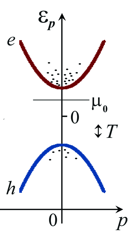
Figure 2: A band diagram of the simplest two-component electron-hole system with the symmetric quadratic dispersion laws and the non-degenerate statistics.

If $\mu_{0},T\ll\Delta$, the particles of the both types form non-degenerate Boltzmann gases. For simplicity, we will use the formulas for the non-degenerate gase up to the values of the chemical potential $\mu_{0},T\lesssim\Delta/2$, when some corrections to the all formulas due to the Pauli principle arise. Such an approximation corresponds in its accuracy to the neglect, made in the previous section, of the dependencies of the function $f$ and the particle velocity $v$ on the particle energy $\varepsilon$.

We again consider a flow in a long sample with the length $L$ and the width $W\ll L$. The sample edges is supposed to be rough and the scattering of particle on the edges is fully diffusive. In this section we present the results only for the very long samples, $L\gg 1/\gamma_{m}$, where $\gamma_{m}$ is the minimum value of the scattering rates in the system.

The kinetic equation for a two-component system in the simplest approximation used in the previous section for a one-component system takes the form:

$$\begin{array}[]{c}\displaystyle\cos\varphi\,\frac{\partial f^{\alpha}}{\partial y}-\sin\varphi\,e^{\alpha}E_{0}-\cos\varphi\,e^{\alpha}E_{H}+\\ \\ \displaystyle\qquad\qquad+\omega_{c}^{\alpha}\,\frac{\partial f^{\alpha}}{\partial\varphi}=\mathrm{St}^{\alpha\alpha}[\,f^{\alpha}\,]+\mathrm{St}^{\alpha\overline{\alpha}}[\,f^{\alpha},f^{\overline{\alpha}}\,\,]\>,\end{array}$$ (37)

where the superscript $\alpha=h,e$ denotes the type of particles: $\alpha=h$ for holes and $\alpha=e$ for electrons; $\overline{\alpha}=e$ for $\alpha=h$ and $\overline{\alpha}=h$ for $\alpha=e$; $e^{h,e}=\pm e_{0}$, $e_{0}$ is the absolute value of the electron charge; $\omega_{c}^{\alpha}=e^{\alpha}B/mc$. The collision integrals

$$\mathrm{St}^{\alpha\alpha}[f^{\alpha}]=\gamma^{\alpha}(f^{\alpha}-P[f^{\alpha}\,])$$ (38)

describe electron-electron and hole-hole collisions, both conserving momentum and leading to forming hydrodynamic electron and hole flows (if only one component of the electron-hole fluid is present). The collision integrals

$$\mathrm{St}^{\alpha\overline{\alpha}}\,[\,f^{\alpha},f^{\overline{\alpha}}\,\,]=\gamma^{\alpha\overline{\alpha}}(f^{\alpha}-P[f^{\overline{\alpha}}\,\,]\,)$$ (39)

describe electron-hole collisions, which also conserve the total momentum, but lead to a finite Ohmic resistance for an electron-hole system in electric field (due to opposite direction of the electric forces acting on electrons and on holes). For the relaxation rates in a symmetric non-degenerated electron-hole system shown at Fig. 2 we have: $\gamma^{\alpha}=\Gamma n_{0}^{\alpha}$ and $\gamma^{\alpha\overline{\alpha}}=\Gamma n_{0}^{\overline{\alpha}}$, where $n_{0}^{h,e}=T\nu e^{-\Delta/(2T)\mp\mu_{0}/T}$ are the equilibrium particle densities, $\Gamma$ is a parameter independent on the densities $n_{0}^{\alpha}$, $\nu=gm/(2\pi\hbar^{2})$ is the 2D density of states for the particles with a quadratic spectrum, and $g$ is the spin-valley degeneracy.

As it has been done for a one-component system, the kinetic equation (37) can be rewritten in the form:

$$\begin{array}[]{c}\displaystyle\Big{[}\cos\varphi\,\frac{\partial}{\partial y}+\gamma\Big{]}\widetilde{f}^{\alpha}-\sin\varphi\,e^{\alpha}E_{0}=\\ \\ \displaystyle\qquad\qquad=\gamma^{\alpha}P[\widetilde{f}^{\alpha}]+\gamma^{\alpha\overline{\alpha}}P[\,\widetilde{f}^{\,\overline{\alpha}}\,]-\omega_{c}^{\alpha}\,\frac{\partial\widetilde{f}^{\alpha}}{\partial\varphi}\end{array}\>,$$ (40)

where the terms in the right part should be considered as small perturbations to the left part. In Eq. (40) we introduced the notations $\widetilde{f}^{\alpha}=f^{\alpha}+e^{\alpha}\phi$ and $\gamma=\gamma^{\alpha}+\gamma^{\alpha\overline{\alpha}}=\Gamma(n_{0}^{e}+n_{0}^{h})$. For brevity, we again omit the tilde in the functions $\widetilde{f}^{\alpha}$ and further write just $f^{\alpha}\equiv\widetilde{f}^{\alpha}$.

III.2 Magnetotransport and electrostatics

We see that the left part of Eq. (40) and the magnetic field term in its right part are identical with the ones of Eq. (5). Thus the expressions for the main parts of the distribution function $f_{0}$ and the current density $j_{0}$ as well as for the magnetic field corrections $f_{1}\sim\omega_{c}$ and $f_{2}\sim\omega_{c}^{2}$ obtained in the previous section for a one-component systems remains valid for each of the both electron and hole components of the two-component system. In this way, we have:

$$j_{0}^{\alpha}=\frac{2n^{\alpha}_{0}e^{\alpha}E_{0}W}{\pi m}\,\ln\Big{(}\frac{1}{\gamma W}\Big{)}\>,$$ (41)

$$I_{0}=\frac{2e_{0}^{2}(n_{0}^{h}+n_{0}^{e})E_{0}W^{2}}{\pi m}\,\ln\Big{(}\frac{1}{\gamma W}\Big{)}\>,$$ (42)

$$\Delta I=\frac{3e_{0}^{2}(n^{h}+n^{e}_{0})E_{0}}{2\pi m}\frac{\omega_{c}^{2}}{\gamma^{4}}\>,$$ (43)

and

$$(f_{1}^{\alpha})^{m=0}=-\frac{\omega_{c}e_{0}E_{0}}{\pi}\,Wy\,\ln\Big{(}\frac{1}{\gamma W}\Big{)}\>,$$ (44)

where $\omega_{c}=|\omega_{c}^{\alpha}|$. We see from Eq. (41) that the hole and the electron flows have opposite directions: $j_{0}^{h,e}\sim\pm n^{h,e}_{0}$. The formulas (42) and (43) leads to the negative magnetoresistance identical to the magnetoresistance (28) in a one-component system.

If $\mu_{0}=0$ the electron-hole system becomes fully symmetric relative to the operation of replacing of electrons by holes and changing the directions of all the fields. In particular, the charge density is equal to zero as $n_{0}^{e}=n_{0}^{h}$ and $\delta n^{e}=\delta n^{h}$. This is the so-called charge-neutrality point. In it the Hall electric field is absent, and the zero harmonic of the magnetic field correction to the distribution function $f_{1}$ is related only to a perturbation of the total particle density $\delta n^{e}+\delta n^{h}$.

At the gate voltages corresponding to small values of the equilibrium chemical potential, $\mu_{0}\ll T,\Delta$, the electron and the hole components of the system as well as their responses on the external fields are almost symmetrical. In particular, the electrons and the hole equilibrium densities $n_{0}^{e}$ and $n_{0}^{h}$ as well as their perturbations $\delta n^{e}$ and $\delta n^{h}$ are close one to another: $|n_{0}^{e}-n_{0}^{h}|\ll n_{0}^{e,h}$ and $|\delta n^{e}-\delta n^{h}|\ll|\delta n^{e,h}|$. In such situation, the zero harmonic $(f_{1}^{\alpha})^{m=0}$ of the distribution function is related to both a perturbation of the particle density $\delta\varrho$ and arising of a charge density $e_{0}(\delta n^{h}-\delta n^{e})$ (related to the Hall electric field):

$$(f_{1}^{\alpha})^{m=0}=\delta\mu^{\alpha}+e^{\alpha}\phi\>,$$ (45)

where $\delta\mu^{\alpha}$ are the perturbations of the electron and the hole chemical potentials and $\phi$ is the electrostatic potential corresponding to the charge density $e_{0}(\delta n^{h}-\delta n^{e})$. Using Eqs. (45) and (44) one can calculate the perturbations of the particle densities

$$\delta n^{h,e}=\nu\,\delta\mu^{h,e}\exp\Big{(}\displaystyle-\frac{\Delta}{2T}\mp\frac{\mu_{0}}{T}\Big{)}$$ (46)

and the Hall electric field $E_{H}=-\phi^{\prime}$ in a vicinity as well as far from the charge neutrality point.

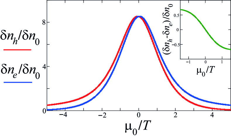
Figure 3: The dependence of the perturbations of the hole and electron densities $\delta n_{h}$ and $\delta n_{e}$ at the sample edge $y=-W/2$ on the equilibrium chemical potential $\mu_{0}$. Inset shows the difference $(\delta n_{h}-\delta n_{e})|_{y=-W/2}/\delta n_{0}$ which is proportional to the charge density and the Hall electric field $E_{H}$. All curves are plotted for the following parameters: $\gamma|_{\mu_{0}=0}W=2\cdot 10^{-4}$ and $D=10$.

We describe the electrostatics of the two-component system and the metallic gate within the gradual channel approximation, in which the electrostatic potential $\phi$ is related to the charge density in the 2D layer as:

$$\phi(y)=\frac{4\pi e_{0}d}{\kappa}\,[\,\delta n^{h}(y)-\delta n^{e}(y)\,]\>.$$ (47)

Here $\kappa$ is the background dielectric constant and $d$ is the distance between the 2D layer and the gate, which should be much greater than the Bohr $a_{B}$ and the Debye $r_{D}$ radii of 2D particles. Solving the system of equations (44), (45), and (47) for $\delta\mu^{e}$, $\delta\mu^{h}$ and $\phi$, we obtain:

$$\frac{\delta n^{h,e}(y,\mu_{0})}{\delta n_{0}}=-\frac{D+e^{\mp\mu_{0}/T}/2}{D\cosh(\mu_{0}/T)}\,\frac{y}{W}\,\ln\Big{(}\frac{1}{\gamma W}\Big{)}\>,$$ (48)

where the parameter $D$,

$$D=\frac{2gd}{a_{B}}\exp\Big{(}\displaystyle-\frac{\Delta}{2T}\Big{)}$$ (49)

is considered to be much greater than unity (it is possible as $d\gg a_{B}$) and the amplitude

$$\delta n_{0}=\frac{\omega_{c}e_{0}E_{0}W^{2}}{\pi}\,\,\nu\,\exp\Big{(}\displaystyle-\frac{\Delta}{2T}\Big{)}$$ (50)

does not depend on $\mu_{0}$. For the Hall electric field, $E_{H}=-\phi^{\prime}=const(y)$, we obtain from (47) and (48):

$$E_{H}(\mu_{0})=-\frac{\omega_{c}WE_{0}}{\pi}\,\,\tanh\Big{(}\frac{\mu_{0}}{T}\Big{)}\,\ln\Big{(}\frac{1}{\gamma W}\Big{)}\>.$$ (51)

In Fig. 3 we plotted the values $\delta n^{h,e}$ at the sample edge $y=-W/2$ as functions of the equlibrium chemical potential $\mu_{0}$ with taking into account the dependence of the rate $\gamma=\gamma^{\alpha\alpha}+\gamma^{\alpha\overline{\alpha}}$ on the equilibrium densities $n_{0}^{\alpha}=n_{0}^{\alpha}(\mu_{0})$. We see that near the charge neutrality point, $\mu_{0}=0$, the perturbation of the electron and hole densities are close one to another, while with the removal of $\mu_{0}$ from the point $\mu_{0}=0$ the electron and hole densities are very different and the Hall electric field (51) approaches to the result (24) obtained in the previous section for a one-component system.

III.3 Hydrodynamic and Ohmic corrections

From the kinetic equations in the form (40) one can calculate the hydrodynamic and the Ohmic corrections to the current and the Hall electric field related to the arrival part of collision integrals $\mathrm{St}^{\alpha\alpha}$ and $\mathrm{St}^{\alpha\overline{\alpha}}$, respectively. The terms “hydrodynamic” and “Ohmic corrections” have following origins. Due to opposite signs of the electron and the hole charges, $e^{e,h}=\mp e_{0}$, the particle flows $j_{0}^{e}$ and $j_{0}^{h}$ have opposite directions [see Eq. (41)]. Thus the corrections to the particle flows $j_{0}^{\alpha}$ due to the arrival terms $\gamma^{\alpha}P[f^{\alpha}]$ are co-directed with $j_{0}^{\alpha}$, while the corrections to $j_{0}^{\alpha}$ from the departure terms $\gamma^{\alpha\overline{\alpha}}P[f^{\overline{\alpha}}\,]$ have the opposite directions relative to the directions of $j_{0}^{\alpha}$ In this way, the corrections of the first type, increasing the current, should be treated as a precursor of forming the Poiseuille viscous flow, while the second type corrections, decreasing the current and increasing the sample resistance, are a precursor of forming of a homogeneous Ohmic flow.

Using the method described in of the previous section, we obtained the correction to the total current in zero magnetic field:

$$\delta I_{h}=\frac{4e_{0}^{2}E_{0}\Gamma W^{3}}{\pi^{2}m}\,\big{(}n_{0}^{h}-n_{0}^{e}\big{)}^{2}\,\ln^{2}\Big{(}\frac{1}{\gamma W}\Big{)}\>,$$ (52)

the correction to the Hall electric field:

$$\Delta E_{H}=\frac{4\omega_{c}\Gamma W^{2}E_{0}}{\pi^{2}}\,(n_{0}^{h}-n_{0}^{e})\,\ln^{2}\Big{(}\frac{1}{\gamma W}\Big{)}\>,$$ (53)

and the correction to the magnetic-field dependent part of the total current:

$$\Delta I_{2}=\frac{6e_{0}^{2}E_{0}\omega_{c}^{2}\Gamma W}{\pi^{2}m\gamma^{4}}\,\big{(}n_{0}^{h}-n_{0}^{e}\big{)}^{2}\,\ln\Big{(}\frac{1}{\gamma W}\Big{)}\>.$$ (54)

It is noteworthy that all the obtained correction vanish at the charge neutrality point when $\mu_{0}=0$ and $n_{0}^{h}=n_{0}^{e}$. and the corrections to the current (52) and (54) are always positive. This means that the electron-electron and electron-hole collisions in a non-degenerate symmetric two-component system lead together to the hydrodynamic (but not to the Ohmic) reconstruction of the ballistic flow. This effect however vanishes at the charge neutrality point when these two types of scattering compensate each other.

IV Acknowledgements

We are grateful to A. I. Chugunov, A. P. Dmitriev, M. M. Glazov, I. V. Gornyi, and V. Yu. Kachorovskii for valuable discussions as well as to A. P. Alekseeva, E. G. Alekseeva, I. P. Alekseeva, N. S. Averkiev, A. I. Chugunov, I. V. Gornyi, M. M. Glazov, and D. S. Svinkin for advice and support.

This work was supported by the Russian Fund for Basic Research (Grants No. 16-02-01166-a and 17-02-00217-a) and by the grant of the Basis Foundation (Grant No. 17-14-414-1).

References

- (1) R. N. Gurzhi, Sov. Phys. Uspekhi 94, 657 (1968).
- (2) C. W. J. Beenakker and H. van Houten, Quantum Transport in Semiconductor Nanostructures (review), Solid State Physics 44, 1 (1991); arXiv:cond-mat/0412664v1 (2004).
- (3) A. T. Hatke, M. A. Zudov, J. L. Reno, L. N. Pfeiffer, and K. W. West, Phys. Rev. B 85, 081304 (2012).
- (4) R. G. Mani, A. Kriisa, and W. Wegscheider, Scientific reports 3, 2747 (2013).
- (5) L. Bockhorn, P. Barthold, D. Schuh, W. Wegscheider, and R. J. Haug, Phys. Rev. B 83, 113301 (2011).
- (6) Q. Shi, P. D. Martin, Q. A. Ebner, M. A. Zudov, L. N. Pfeiffer, and K. W. West, Phys. Rev. B 89, 201301 (2014).
- (7) L. Bockhorn, I. V. Gornyi, D. Schuh, C. Reichl, W. Wegscheider, and R. J. Haug, Phys. Rev. B 90, 165434 (2014).
- (8) P. J. W. Moll, P. Kushwaha, N. Nandi, B. Schmidt, and A. P. Mackenzie, Science 351, 1061 (2016).
- (9) J. Gooth, F. Menges, C. Shekhar, V. Suess, N. Kumar, Y. Sun, U. Drechsler, R. Zierold, C. Felser, B. Gotsmann arXiv:1706.05925 (2017).
- (10) A. I. Berdyugin, S. G. Xu, F. M. D. Pellegrino, R. Kr- ishna Kumar, A. Principi, I. Torre, M. Ben Shalom, T. Taniguchi, K. Watanabe, I. V. Grigorieva, M. Polini, A. K. Geim, D. A. Bandurin, arXiv:1806.01606 (2018)
- (11) G. M. Gusev, A. D. Levin, E. V. Levinson, and A. K. Bakarov, AIP Advances 8, 025318 (2018).
- (12) D. A. Bandurin, I. Torre, R. Krishna Kumar, M. Ben Shalom, A. Tomadin, A. Principi, G. H. Auton, E. Khestanova, K. S. NovoseIov, I. V. Grigorieva, L. A. Ponomarenko, A. K. Geim, and M. Polini, Science 351, 1055 (2016).
- (13) R. Krishna Kumar, D. A. Bandurin, F. M. D. Pellegrino, Y. Cao, A. Principi, H. Guo, G. H. Auton, M. Ben Shalom, L. A. Ponomarenko, G. Falkovich, K. Watanabe, T. Taniguchi, I. V. Grigorieva, L. S. Levitov, M. Polini, and A. K. Geim, Nature Physics 13, 1182 (2017).
- (14) A. D. Levin, G. M. Gusev, E. V. Levinson, Z. D. Kvon, and A. K. Bakarov, Phys. Rev. B 97, 245308 (2018).
- (15) G. M. Gusev, A. D. Levin, E. V. Levinson, and A. K. Bakarov, Phys. Rev. B 98, 161303 (2018).
- (16) J.-U.Lee, D. Yoon, H. Kim, S.W. Lee, H. Cheong, Phys. Rev. B 83, 081419 (2011).
- (17) S. Yigen and A. R. Champagne, Nano Lett. 14, 289 (2014).
- (18) G. Fugallo, A. Cepellotti, L. Paulatto, et., al, Nano Lett. 14, 6109 (2014).
- (19) X. Xu, L. F. C. Pereira, Y. Wang, J. Wu, K. Zhang, X. Zhao, S. Bae, C. T. Bui, R. Xie, J. T. L. Thong, B. H. Hong, K. P. Loh, D. Donadio, B. Li, and B. Ozyilmaz, Nat. Commun. 5, 3689 (2014).
- (20) M. Hruska and B. Spivak, Phys. Rev. B 65, 033315 (2002).
- (21) M. Muller, L. Fritz, S. Sachdev, Phys. Rev.B 78, 115406 (2008).
- (22) A. V. Andreev, S. A. Kivelson, and B. Spivak, Phys. Rev. Lett. 106, 256804 (2011).
- (23) M. Mendoza, H. J. Herrmann, and S. Succi, Scientic re- ports 3, 1052 (2013).
- (24) A. Tomadin, G. Vignale, and M. Polini, Phys. Rev. Lett. 113, 235901 (2014).
- (25) I. Torre, A. Tomadin, A. K. Geim, M. Polini, Phys. Rev. B 92, 165433 (2015).
- (26) B. N. Narozhny, I. V. Gornyi, M. Titov, M. Schutt, and A. D. Mirlin, Phys. Rev. B 91, 035414 (2015).
- (27) P. S. Alekseev, Phys. Rev. Lett. 117, 166601 (2016).
- (28) L. Levitov and G. Falkovich, Nature Physics 12, 672 (2016).
- (29) H. Guo, E. Ilseven, G. Falkovich, L. Levitov, PNAS 114, 3068 (2017).
- (30) A. Lucas, Phys. Rev. B 95 115425 (2017); A. Lucas and K.C. Fong, Journal of Physics: Condensed Matter 30, 053001 (2018).
- (31) A. Lucas and S. A. Hartnoll, Phys. Rev. B 97, 045105 (2018).
- (32) V. Scopelliti, K. Schalm, and A. Lucas, Phys. Rev. B 96, 075150 (2017).
- (33) F. M. D. Pellegrino, I. Torre, and M. Polini, Phys. Rev. B 96, 195401 (2017).
- (34) P. S. Alekseev, A. P. Dmitriev, I. V. Gornyi, V. Y. Kachorovskii, B. N. Narozhny, M. Schutt, M. Titov, Phys. Rev. Lett. 114, 156601 (2015).
- (35) G. Y. Vasileva, D. Smirnov, Y. L. Ivanov, Y. B. Vasilyev, P. S. Alekseev, A. P. Dmitriev, I. V. Gornyi, V. Y. Kachorovskii, M. Titov, B. N. Narozhny, R. J. Haug, Phys. Rev. B 93, 195430 (2016).
- (36) P. S. Alekseev, A. P. Dmitriev, I. V. Gornyi, V. Y. Kachorovskii, B. N. Narozhny, M. Schutt, M. Titov, Phys. Rev. B 95, 165410 (2017).
- (37) P. S. Alekseev, A. P. Dmitriev, I. V. Gornyi, V. Y. Kachorovskii, M. A. Semina, Semiconductors 51, 766 (2017).
- (38) P. S. Alekseev, A. P. Dmitriev, I. V. Gornyi, V. Yu. Kachorovskii, B. N. Narozhny, and M. Titov, Phys. Rev. B 97, 085109 (2018).
- (39) P. S. Alekseev, A. P. Dmitriev, I. V. Gornyi, V. Yu. Kachorovskii, B. N. Narozhny, and M. Titov, Phys. Rev. B 98, 125111 (2018).
- (40) S. Lee, D. Broido, K. Esfarjani, G. Chen, Nat. Comm. 6, 6290 (2015).
- (41) A. Cepellotti, G. Fugallo, L. Paulatto, M. Lazzeri, F. Mauri, N. Marzari, Nat. Comm. 6, 6400 (2015).
- (42) K. H. Michel, P. Scuracchio, and F. M. Peeters, Phys. Rev. B 96, 094302 (2017).
- (43) O. Kashuba, B. Trauzettel, L. W. Molenkamp, Phys. Rev. B 97, 205129 (2018).
- (44) T. Scaffidi, N. Nandi, B. Schmidt, A. P. Mackenzie, J. E. Moore, Phys. Rev. Lett. 118, 226601 (2017).
- (45) P. S. Alekseev and M. A. Semina, Phys. Rev. B 98, 165412 (2018).
- (46) E. I. Kiselev and J. Schmalian, arXiv: 1806.03933v3 (2018).
- (47) R. Moessner, P. Surowka, P. Witkowski, Phys. Rev. B 97, 161112 (2018).
- (48) M. Semenyakin and G. Falkovich, Phys. Rev. B 97, 085127 (2018).
- (49) R. Cohen and M. Goldstein, arXiv 1809.05847v1 (2018).
- (50) T. Holder, R. Queiroz, T. Scaffidi, N. Silberstein, A. Rozen, J. A. Sulpizio, L. Ella, S. Ilani, and A. Stern, arXiv:1901.08546 (2019).
- (51) T. Holder, R. Queiroz, and A. Stern, arXiv:1903.05541 (2019).
- (52) For ease of reading, we present in this paper the model for the ballistic transport of interaction particles formulated in Ref. ours_bal as well as some of the results obtained in that work. Herewith in this paper, unlike Ref. ours_bal , the definitions of the current density and the total current are given with the dimensional coefficients: the unperturbed particle density , the particl charge and the mass .
- (53) M. N. Kogan, Rarefied Gas Dynamics (Springer, New York, 1969).
- (54) P. S. Alekseev, Phys. Rev. B 98, 165440 (2018).
- (55) Here the expression for is written with an exact numeric factor, while the expression for magnetoresistance is written only up to an order of magnitude. The reason of this difference is as follows. The expression for is obtained by integrating of the contributions from electrons with the angles close to and having a logarithmic divergence by , while the expression for (and thus for ) is obtained by integrating of the contributions with the divergence at the same angles , but having a stronger (not logarithmic) power singularity. The last does not allow to determine (when truncating the integration at ) the numerical prefactor in and, thus, in .