Reciprocal Best Match Graphs

Abstract

Reciprocal best matches play an important role in numerous applications in computational biology, in particular as the basis of many widely used tools for orthology assessment. Nevertheless, very little is known about their mathematical structure. Here, we investigate the structure of reciprocal best match graphs (RBMGs). In order to abstract from the details of measuring distances, we define reciprocal best matches here as pairwise most closely related leaves in a gene tree, arguing that conceptually this is the notion that is pragmatically approximated by distance- or similarity-based heuristics. We start by showing that a graph $G$ is an RBMG if and only if its quotient graph w.r.t. a certain thinness relation is an RBMG. Furthermore, it is necessary and sufficient that all connected components of $G$ are RBMGs. The main result of this contribution is a complete characterization of RBMGs with 3 colors/species that can be checked in polynomial time. For 3 colors, there are three distinct classes of trees that are related to the structure of the phylogenetic trees explaining them. We derive an approach to recognize RBMGs with an arbitrary number of colors; it remains open however, whether a polynomial-time for RBMG recognition exists. In addition, we show that RBMGs that at the same time are cographs (co-RBMGs) can be recognized in polynomial time. Co-RBMGs are characterized in terms of hierarchically colored cographs, a particular class of vertex colored cographs that is introduced here. The (least resolved) trees that explain co-RBMGs can be constructed in polynomial time.

Keywords: Pairwise best hit reciprocal best match heuristics vertex colored graph phylogenetic tree hierarchically colored cograph

1 Introduction

An important task in computational biology is the annotation of newly sequenced genomes, and in particular to establish correspondences between orthologous genes. Two genes $x$ and $y$ in two different species $s$ and $t$, respectively, are orthologs if their last common ancestor was the speciation event that separated the lineages of $s$ and $t$ (Fitch, 2000). A large class of software tools for orthology assignment are based on the pairwise reciprocal best match heuristic: the genes $x$ and $y$ are (candidate) orthologs if $y$ is a best match in terms of sequence similarity to $x$ among all genes from species $t$, and $x$ is a best match to $y$ among all genes from $s$. This approach, which has been termed Symmetric Best Match (Tatusov et al., 1997), bidirectional best hits (BBH) (Overbeek et al., 1999), reciprocal best hits (RBH) (Bork et al., 1998), or reciprocal smallest distance (RSD) (Wall et al., 2003), provides orthology assignments on par with elaborate phylogeny-based methods, see Altenhoff and Dessimoz (2009); Altenhoff et al. (2016); Setubal and Stadler (2018) for reviews and benchmarks.

The application of pairwise best hits methods to orthology detection relies on the observation that given a gene $x$ in species $r$ (and disregarding horizontal gene transfer), all its co-orthologous genes $y$ in species $s$ are by definition closest relatives of $x$. Since orthology is a symmetric relation, orthologs are necessarily reciprocal best matches (RBMs). In practice, however, reciprocal best matches are approximated by sequence similarities, making the tacit assumption that the molecular clock hypothesis is not violated too dramatically, see Geiß et al. (2019b) for a more detailed discussion. Modern orthology detection tools are well aware of the shortcoming of pairwise best sequence similarity estimates and employ additional information, in particular synteny (Lechner et al., 2014; Jahangiri-Tazehkand et al., 2017), or use small subsets of pairwise matches to identify erroneous orthology assignments (Yu et al., 2011; Train et al., 2017). In this contribution we will not concern ourselves with the practicalities of inferring best matches. Instead, we will focus on the best match relation from a mathematical point of view.

Despite its practical importance, very little is known about the RBM relation. Like orthology, RBMs are a phylogenetic concept and thus refer to a phylogenetic tree $T$. Denote by $L$ the leaf set of $T$ and consider a surjective map $\sigma:L\to S$ that assigns to each gene $x\in L$ the species $\sigma(x)\in S$ within which $x$ resides. To avoid trivial cases, we assume that there are $|S|>1$ species. In this setting we can express the concept of RBMs by

Definition 1.

The leaf $y$ is a best match of the leaf $x$ in the gene tree $T$ if and only if $\operatorname{lca}(x,y)\preceq\operatorname{lca}(x,y^{\prime})$ for all leaves $y^{\prime}$ with $\sigma(y^{\prime})=\sigma(y)$. If $x$ is also a best match of $y$, we call $x$ and $y$ reciprocal best matches.

As usual, $\operatorname{lca}_{T}(x,y)$ denotes the last common ancestor of $x$ and $y$ on $T$, and $\preceq_{T}$ is the ancestor order on the vertices of $T$, where the root of $T$ is the unique maximal element. We omit the index $T$ whenever the context is clear. The reciprocal best match relation is symmetric by definition. It is reflexive because every gene $x$ in species $s$ is its own (unique) best match within $s$.

The best match relation and the reciprocal best match relation are conveniently represented as a vertex colored digraph $(\mathaccent 382{G},\sigma)$ and vertex colored undirected graph $(G,\sigma)$, respectively, with vertex set $L$. Arcs and edges represent best matches and reciprocal best matches, respectively. Since there is a 1-1 relationship between graphs with a loop at each vertex and graphs without loops, consider $(\mathaccent 382{G},\sigma)$ and $(G,\sigma)$ as loop-less. The relationship between these graphs and the trees from which they are derived is captured by

Definition 2.

Let $(T,\sigma)$ be a tree with leaf set $L$, let $\mathaccent 382{G}=(L,\mathaccent 382{E})$ be a digraph and $G=(L,E)$ an undirected graph, both with vertex set $L$, and let $\sigma:L\to S$ be a map with $|S|\geq 2$. Then, $(T,\sigma)$ explains $(\mathaccent 382{G},\sigma)$ if there is an arc $(x,y)\in\mathaccent 382{E}$ in $\mathaccent 382{G}$ precisely if $y$ is a best match of $x$ in $(T,\sigma)$ with $\sigma(x)\neq\sigma(y)$. Analogously, $(T,\sigma)$ explains $(G,\sigma)$ if there is an edge $xy\in E$ in $G$ precisely if $x$ and $y$ form a reciprocal best match in $(T,\sigma)$ with $\sigma(x)\neq\sigma(y)$.

Def. 2 gives rise to two classes of vertex colored graphs:

Definition 3.

A vertex colored digraph $(\mathaccent 382{G},\sigma)$ is a best match graph (BMG) if there exists a leaf-colored tree $(T,\sigma)$ that explains $(\mathaccent 382{G},\sigma)$. An undirected graph $(G,\sigma)$ is a reciprocal best match graph (RBMG) if there exists a leaf-colored tree $(T,\sigma)$ that explains $(G,\sigma)$.

For BMGs we recently reported two different characterizations and corresponding polynomial-time recognition algorithms (Geiß et al., 2019b).

Here we extend the analysis to RBMGs. Since the material is rather extensive (many of the proofs use elementary graph theory but are very technical) we subdivided the presentation in a main narrative text explaining the main results and a second technical part collecting the proofs of the main results as well as additional technical results that are useful for later more practical applications. In order to ensure that the second, technical part of the contribution is self-contained all definitions and results are (re)stated there. In the narrative part we only give those definitions that are necessary to understand the results presented there. We use the same numbering of statements in the narrative and the technical part to facilitate the cross-referencing.

We start in Section 2 to define the concepts that we need here. We follow the general strategy to reduce redundancy by identifying classes of trees explaining the same graphs and equivalence classes of graphs explained by trees with essentially the same structure. We start in Sections 3 in the main text and A in the technical part with the description of least resolved trees as representatives that are sufficient to explain a given RBMG. As it turns out, least resolved trees are not unique in general. Complementarily, in Sections 4 and B we introduce a color-aware thinness relation $\mathsf{S}$ and show that it suffices to characterize $\mathsf{S}$-thin RBMGs. Combining these ideas, we demonstrate in Sections 5 and C that $(G,\sigma)$ is an RBMG if and only if each of its connected components is an RBMG and at least one of them contains all colors, and give a simple construction for a tree explaining $(G,\sigma)$ from trees for the connected components. In order to characterize connected, $\mathsf{S}$-thin RBMGs, we first consider the case of three colors (Sections 6 and D). We find that there are three distinct classes of 3-RBMGs that can be recognized in polynomial time. One of these classes does not contain induced paths on four vertices, so called $P_{4}$s, while the other two classes do. Since $P_{4}$s are at the heart of cograph editing approaches to improve orthology estimates (Hellmuth et al., 2013), we consider these structures in some more detail in Section E of the technical part and characterize three distinct types: good, bad, and ugly $P_{4}$s. In Sections 7 and F we prove that trees explaining an $n$-RBMG can be composed from tree sets explaining the induced 3-RBMGs for all three-color subsets. However, the computational complexity for recognizing $n$-RBMGs is left as an open problem. Because of their practical relevance in orthology detection, we then characterize the $n$-RBMGs that are so-called cographs. As we shall see, the recognition of cograph $n$-RBMGs and the construction of trees that explain them can be done in polynomial time. We finish with a brief survey of potential applications of the results presented here and some open problems.

2 Preliminaries

Throughout this contribution, we say that two sets $P,Q$ do not overlap if $P\cap Q\in\{\emptyset,P,Q\}$, and they overlap, otherwise. We will also assume throughout that the map $\sigma:L\to S$ is surjective. For a subset $L^{\prime}\subseteq L$ we write $\sigma(L^{\prime})=\{\sigma(x)\mid x\in L^{\prime}\}$. Moreover, we use the notation $\sigma_{|L^{\prime}}$ for the surjective map $\sigma:L^{\prime}\to\sigma(L^{\prime})$. We will frequently need to refer to the number $|S|$ of colors and often speak of $|S|$-BMGs and $|S|$-RBMGs.

A phylogenetic tree $T=(V,E)$ (on $L$) is a rooted tree with root $\rho_{T}$, leaf set $L(T)=L\subseteq V$ and inner vertices $V^{0}=V\setminus L$ such that each inner vertex of $T$ (except possibly the root) is of degree at least three. For $x\in V$, we denote by $T(x)$ the subtree rooted at $x$. For a phylogenetic tree $T$ on $L$, the restriction $T_{|L^{\prime}}$ of $T$ to $L^{\prime}\subseteq L$ is the phylogenetic tree with leaf set $L^{\prime}$ that is obtained from $T$ by first taking the minimal subtree of $T$ with leaf set $L^{\prime}$ and then suppressing all vertices of degree two with the exception of the root $\rho_{T_{|L^{\prime}}}$.

Throughout this contribution all rooted trees are assumed to be phylogenetic unless explicitly stated otherwise.

A vertex $u\in V$ is an ancestor of $v\in V$, $u\succeq_{T}v$, and $v$ is a descendant of $u$, $v\preceq_{T}u$, if $u$ lies on the unique path from $v$ to the root $\rho_{T}$. We write $u\succ_{T}v$ ($v\prec_{T}u$) for $u\succeq_{T}v$ ($v\preceq_{T}u$) and $u\neq v$. For a subset $\alpha\subseteq V$ we write $\alpha\preceq_{T}u$ to mean that $x\preceq_{T}u$ for all $x\in\alpha$. If $uv\in E$ and $u\succ_{T}v$, we call $u$ the parent of $v$, denoted by $\mathsf{par}(v)$, and define the children of $u$ as $\mathsf{child}(u)\coloneqq\{v\in V\mid uv\in E\}$. It will be convenient to use the notation $uv\in E$ to indicate $u\succ_{T}v$, i.e., $u$ is closer to the root. Moreover, we say that $e=uv$ is an outer edge if $v\in L$ and an inner edge otherwise.

A tree $T^{\prime}$ is displayed by $T$, denoted by $T^{\prime}\leq T$, if $T^{\prime}$ can be obtained from a subtree of $T$ by a series of edge contractions. For a tree $T$ on $L$ with coloring map $\sigma:L\to S$, in symbols $(T,\sigma)$, we say that $(T,\sigma)$ displays or is a refinement of $(T^{\prime},\sigma^{\prime})$ if $T^{\prime}\leq T$ and $\sigma^{\prime}(v)=\sigma(v)$ for any $v\in L(T^{\prime})\subseteq L$. The subtree $T(v)$ has leaf set $L^{\prime}\coloneqq L(T(v))$ and leaf coloring $\sigma_{L^{\prime}}:L^{\prime}\to\sigma(L^{\prime})$. We write $\operatorname{lca}_{T}(A)$ for the last common ancestor of all elements of a set $A\subseteq V$ of vertices. For a tree $T=(V,E)$ and some inner edge $e=uv$ of $T$, we denote by $T_{e}$ the tree that is obtained from $(T,\sigma)$ by contraction of $e$, i.e., by identifying $u$ and $v$. Analogously, $T_{A}$ is obtained by contracting a sequence of edges $A=(e_{1},\dots,e_{k})\subseteq E$.

A triple is a binary tree on three leaves. We write $xy|z$ if the path from $x$ to $y$ does not intersect the path from $z$ to the root. A set $\mathcal{R}$ of triples is consistent if there is a tree $T$ that displays every triple in $\mathcal{R}$. Analogously, we say that a set of trees $\mathcal{T}$ is consistent it there is a tree $T$ such that $T$ displays every tree $T^{\prime}\in\mathcal{T}$. Consistency of a set of triples $\mathcal{R}$ and more generally trees $\mathcal{T}$ can be decided in polynomial time by explicitly constructing a supertree $T$ (Aho et al., 1981).

In the following, $G=(V,E)$ and $\mathaccent 382{G}=(V,\mathaccent 382{E})$ denote simple undirected and simple directed graphs, respectively. Throughout, we will distinguish directed arcs $(x,y)$ in a digraph $\mathaccent 382{G}$ from edges $xy$ in an undirected graph $G$ or tree $T$. For $x\in V$ we write $N^{+}(x)\coloneqq\{y\in V\mid(x,y)\in\mathaccent 382{E}\}$ for its out-neighborhood and $N^{-}(x)\coloneqq\{y\in V\mid(y,x)\in\mathaccent 382{E}\}$ for its in-neighborhood. The notation naturally extends to sets of vertices $A\subseteq V$: $N^{+}(A)=\bigcup_{x\in A}N^{+}(x)$ and $N^{-}(A)=\bigcup_{x\in A}N^{-}(x)$. Two vertices $x$ and $y$ of $\mathaccent 382{G}$ are in relation $\mathsf{R}$ if $N^{+}(x)=N^{+}(y)$ and $N^{-}(x)=N^{-}(y)$, see e.g. (Hellmuth and Marc, 2015). Obviously $\mathsf{R}$ is an equivalence relation. For each $\mathsf{R}$-class $\alpha$ and every $x\in\alpha$ holds $N^{+}(x)=N^{+}(\alpha)$ and $N^{-}(x)=N^{-}(\alpha)$. The set of all $\mathsf{R}$-classes of $(\mathaccent 382{G},\sigma)$ will be denoted by $\mathcal{N}$, or $\mathcal{N}(\mathaccent 382{G})$.

For a colored di-graph $(\mathaccent 382{G},\sigma)$, we write $N_{s}^{+}(x)\coloneqq\{y\in N^{+}(x)\mid\sigma(y)=s\}$ and $N_{s}^{-}(x)\coloneqq\{y\in N^{-}(x)\mid\sigma(y)=s\}$. Similarly, for an undirected colored graph $(G,\sigma)$ with $G=(V,E)$, we write $N(x)\coloneqq\{y\in V\mid xy\in E\}$ for the neighborhood of some vertex $x\in V$. Moreover, we set $N_{s}(x)\coloneqq\{y\in N(x)\mid\sigma(y)=s\}$.

A connected component of a graph $(G,\sigma)$ is a maximal connected subgraph of $(G,\sigma)$. A digraph is connected whenever its underlying undirected graph (obtained by ignoring the direction of the arcs) is connected. For our purposes it will not be relevant to distinguish two colored graphs $(G,\sigma)$ and $(G^{\prime},\sigma^{\prime})$ that are isomorphic in the usual sense of isomorphic colored graphs, i.e., isomorphic graphs $G$ and $G^{\prime}$ that only differ by a permutation of their vertex-coloring. A vertex coloring $\sigma$ is proper if $xy\in E(G)$ implies $\sigma(x)\neq\sigma(y)$. As an immediate consequence of Def. 2 we have

Observation 1.

If $(G,\sigma)$ is an RBMG, then $\sigma$ is a proper vertex coloring.

As a consequence, $(G,\sigma)$ cannot be explained by a leaf-colored tree unless $\sigma$ is a proper vertex coloring. We may therefore assume throughout this contribution that $(G,\sigma)$ is a properly vertex colored graph. Moreover, for $W\subseteq V(G)$ we denote with G[W] the induced subgraph of $G$ and put $(G,\sigma)[W]\coloneqq(G[W],\sigma_{|W})$.

We write $\langle x_{1}\dots x_{k}\rangle\in\mathscr{P}_{k}$ to denote that the vertices $x_{1},\dots,x_{k}$ form an induced path $P=\langle x_{1}\dots x_{k}\rangle$ on $k$ vertices and with edges $x_{i}x_{i+1}$, $1\leq i\leq k-1$. Analogously, $\langle x_{1}\dots x_{k}\rangle\in\mathscr{C}_{k}$ denotes the fact that the vertices $x_{1},\dots,x_{k}$ induce a cycle $C=\langle x_{1}\dots x_{k}\rangle$ on $k$ vertices with edges $x_{i}x_{i+1}$, $1\leq i\leq k-1$, and $x_{k}x_{1}$. An induced cycle on six vertices is called hexagon. We will write that $\langle x_{1}\dots x_{k}\rangle\in\mathscr{P}_{k}$, resp. $\mathscr{C}_{k}$ is of the form $(\sigma(x_{1}),\dots,\sigma(x_{k}))$ to indicate the vertex colors along induced paths, resp., cycles.

Cographs form a class of undirected graphs that play an important in the context of this contribution. They are defined recursively (Corneil et al., 1981):

Definition 4.

An undirected graph $G$ is a cograph if

• $G=K_{1}$

• $G=H\operatorname{\triangledown}H^{\prime}$, where $H$ and $H^{\prime}$ are cographs and $\operatorname{\triangledown}$ denotes the join,

• $G=H\mathbin{\mathchoice{\leavevmode\vtop{\halign{\hfil$\m@th\displaystyle#$\hfil\cr\cup\cr\cdot\crcr}}}{\leavevmode\vtop{\halign{\hfil$\m@th\textstyle#$\hfil\cr\cup\cr\cdot\crcr}}}{\leavevmode\vtop{\halign{\hfil$\m@th\scriptstyle#$\hfil\cr\cup\cr\cdot\crcr}}}{\leavevmode\vtop{\halign{\hfil$\m@th\scriptscriptstyle#$\hfil\cr\cup\cr\cdot\crcr}}}}H^{\prime}$, where $H$ and $H^{\prime}$ are cograph and $\mathbin{\mathchoice{\leavevmode\vtop{\halign{\hfil$\m@th\displaystyle#$\hfil\cr\cup\cr\cdot\crcr}}}{\leavevmode\vtop{\halign{\hfil$\m@th\textstyle#$\hfil\cr\cup\cr\cdot\crcr}}}{\leavevmode\vtop{\halign{\hfil$\m@th\scriptstyle#$\hfil\cr\cup\cr\cdot\crcr}}}{\leavevmode\vtop{\halign{\hfil$\m@th\scriptscriptstyle#$\hfil\cr\cup\cr\cdot\crcr}}}}$ denotes the disjoint union.

The join of two disjoint graphs $H=(V,E)$ and $H^{\prime}=(V^{\prime},E^{\prime})$ is defined by $H\operatorname{\triangledown}H^{\prime}=(V\cup V^{\prime},E\cup E^{\prime}\cup\{xy\mid x\in V,y\in V^{\prime}\})$, whereas their disjoint union is given by $H\mathbin{\mathchoice{\leavevmode\vtop{\halign{\hfil$\m@th\displaystyle#$\hfil\cr\cup\cr\cdot\crcr}}}{\leavevmode\vtop{\halign{\hfil$\m@th\textstyle#$\hfil\cr\cup\cr\cdot\crcr}}}{\leavevmode\vtop{\halign{\hfil$\m@th\scriptstyle#$\hfil\cr\cup\cr\cdot\crcr}}}{\leavevmode\vtop{\halign{\hfil$\m@th\scriptscriptstyle#$\hfil\cr\cup\cr\cdot\crcr}}}}H^{\prime}=(V\cup V^{\prime},E\cup E^{\prime})$.

A graph is a cograph if and only if does not contain an induced $P_{4}$ (Corneil et al., 1981).

Each cograph $G$ is associated with cotrees $T_{G}$, that is, phylogenetic trees with internal vertices labeled by $0$ or $1$, whose leaves correspond to the vertices of $G$. In $T_{G}$, each subtree rooted at an internal vertex $x$ with label $0$ corresponds to the disjoint union of the subgraphs of $G$ induced by the leaf sets $L(T_{G}(y))$ of the children $y\in\mathsf{child}(x)$ of $x$, and each subtree rooted at an $x$ with label $1$ corresponds to the join of the subgraphs of $G$ induced by the $L(T_{G}(y))$, $y\in\mathsf{child}(x)$. In other words, $(T,t)$ is a cotree for $(G,\sigma)$, if $t(\operatorname{lca}_{T}(x,y))=1$ if and only if $xy\in E(G)$. For each cograph $G$ there is a unique discriminating cotree $T_{G}$ with the property that the labels $0$ and $1$ alternate along each root-leaf path in $T_{G}$ (Corneil et al., 1981). For later reference, we summarize here some of the results in (Hellmuth et al., 2013, Sect. 3).

Proposition 1.

Any cotree of a cograph $G$ is a refinement of the unique discriminating cotree of $G$. In particular $(T_{e},t_{e})$ is a cotree for a cograph $G$ if and only if $(T,t)$ is a cotree for $G$, $e=xy$ is an edge with $t(x)=t(y)$ that is contracted to vertex $v_{e}$ in $T_{e}$ and $t_{e}(v_{e})=t(x)$ and $t_{e}(v)=t(v)$ for all remaining vertices.

3 Least Resolved Trees

In this section we consider a notion of “smallest” trees explaining a given RBMG. A we shall see, the characterization of these trees is closely related to the one of best matches but cannot be expressed in terms of reciprocal best matches alone. Throughout this work, the vertex set of BMGs and RBMGs as well as the leaf set of the trees that explain them will be denoted by $L$ and we will write

$$L[s]\coloneqq\{x\mid x\in L,\sigma(x)=s\}$$

for the subset of vertices with color $s\in S$.

Given a leaf-colored tree $(T,\sigma)$, one can easily derive the respective BMG $\mathaccent 382{G}(T,\sigma)$ and RBMG $G(T,\sigma)$ that are explained by $(T,\sigma)$. Conversely, if $(G,\sigma)$ is an RBMG, then there is a tree $(T,\sigma)$ that explains $(G,\sigma)$. This tree also explains the digraph $\mathaccent 382{G}(T,\sigma)$ with the property that $xy\in E(G)$ if and only if both $(x,y)$ and $(y,x)$ are arcs in $\mathaccent 382{G}(T,\sigma)$. A colored graph $(G,\sigma)$ therefore is an RBMG if and only if it is the symmetric part of some BMG.

It is important to note that distinct trees $(T^{\prime},\sigma)$ and $(T^{\prime\prime},\sigma)$ may explain the same RBMG, i.e., $G(T^{\prime},\sigma)=G(T^{\prime\prime},\sigma)$, albeit the leaf-set $L$ and the leaf-coloring $\sigma$ of course must be the same. In general the BMGs $\mathaccent 382{G}(T^{\prime},\sigma)$ and $\mathaccent 382{G}(T^{\prime\prime},\sigma)$ can also be different, even if $G(T^{\prime},\sigma)=G(T^{\prime\prime},\sigma)$. For an example, consider the RBMG $(G,\sigma)$ and the two distinct trees $(T_{e},\sigma)$ and $(T_{f},\sigma)$ in Fig. 1. We have $(G,\sigma)=G(T_{e},\sigma)=G(T_{f},\sigma)$. However, $\mathaccent 382{G}(T_{e},\sigma)$ contains the arc $(a,b^{\prime})$ which is not contained in $\mathaccent 382{G}(T_{f},\sigma)$. Hence, $\mathaccent 382{G}(T_{e},\sigma)\neq\mathaccent 382{G}(T_{f},\sigma)$.

Nevertheless, some properties of BMGs will be helpful as a means to gaining insights into the structure of RBMGs. To this end we briefly recall some pertinent results by Geiß et al. (2019b).

Lemma 1.

Let $(\mathaccent 382{G},\sigma)$ be a BMG with vertex set $L$. Then, $x\mathsf{R}y$ implies $\sigma(x)=\sigma(y)$. In particular, $(\mathaccent 382{G},\sigma)$ has no arcs between vertices within the same $\mathsf{R}$-class. Moreover, $N^{+}(x)\neq\emptyset$, while the in-neighborhood $N^{-}(x)$ may be empty for all $x\in L$.

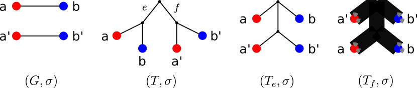
Figure 1: The reciprocal best match graph $(G,\sigma)$ on two colors (red and blue) is explained by $(T,\sigma)$ which contains the redundant edges $e$ and $f$. Contraction of one of these edges gives $(T_{e},\sigma)$ and $(T_{f},\sigma)$, respectively, which are both least resolved but distinct from each other, i.e., there exists no unique least resolved tree w.r.t. $(G,\sigma)$. In particular, none of the trees $(T_{ef},\sigma)$ and $(T_{fe},\sigma)$ explains $(G,\sigma)$.

Although there are in general many different trees that explain the same BMG or RBMG, it is shown by Geiß et al. (2019b) that every BMG $(\mathaccent 382{G},\sigma)$ is explained by a uniquely defined “smallest” tree, its so called least resolved tree. The notion of least resolved trees are also of interest for RBMGs even though we shall see below that they are not unique in the reciprocal setting.

Definition 5.

Let $(G,\sigma)$ be an RBMG that is explained by a tree $(T,\sigma)$. An inner edge $e$ is called redundant if $(T_{e},\sigma)$ also explains $(G,\sigma)$, otherwise $e$ is called relevant.

Lemma 2 in the technical part provides a characterization of redundant edges. It is interesting to note that this characterization of redundancy (w.r.t. an RBMG) of edges in $(T,\sigma)$ requires information on (directed) best matches and apparently cannot be expressed entirely in terms of the reciprocal best match relation.

Definition 6.

Let $(G,\sigma)$ be an RBMG explained by $(T,\sigma)$. Then $(T,\sigma)$ is least resolved w.r.t. $(G,\sigma)$ if $(T_{A},\sigma)$ does not explain $(G,\sigma)$ for any non-empty series of edges $A$ of $(T,\sigma)$.

Given two distinct redundant edges $e\neq f$ of $(T,\sigma)$, the edge $f$ is not necessarily redundant in $(T_{e},\sigma)$, i.e., the tree $(T_{ef},\sigma)$ obtained by sequential contraction of $e$ and $f$ does not necessarily explain $(G,\sigma)$. This in particular implies that the contraction of all redundant edges of $(T,\sigma)$ does not necessarily result in a least resolved tree for the same RBMG. Moreover, there may be more than one least resolved tree that explains a given $n$-RBMG $(G,\sigma)$. Fig. 1 gives an example of least resolved trees that are not unique. The following theorem summarizes some key properties of least resolved trees.

Theorem 1.

Let $(G,\sigma)$ be an RBMG explained by $(T,\sigma)$. Then there exists a (not necessarily unique) least resolved tree $(T_{e_{1}\dots e_{k}},\sigma)$ explaining $(G,\sigma)$ obtained from $(T,\sigma)$ by a series of edge contractions $e_{1}e_{2}\dots e_{k}$ such that the edge $e_{1}$ is redundant in $(T,\sigma)$ and $e_{i+1}$ is redundant in $(T_{e_{1}\dots e_{i}},\sigma)$ for $i\in\{1,\dots,k-1\}$. In particular, $(T,\sigma)$ displays $(T_{e_{1}\dots e_{k}},\sigma)$.

We will return to least resolved trees in Section 7.1, where the concept will be needed as a means to construct a tree explaining an $n$-RBMG from sets of least resolved trees that explain the induced 3-RBMGs for all subsets on three colors.

4 $\mathsf{S}$-Thinness

The $\mathsf{R}$ relation introduced in the previous sections is the natural generalization of thinness in undirected graphs (McKenzie, 1971). As an immediate consequence of Lemma 1, all vertices within an $\mathsf{R}$-class of a BMG have the same color. However, a corresponding result does not hold for RBMGs. Fig. 2 shows a counterexample, where $N(a)=N(b)$ holds for vertices with different colors $\sigma(a)\neq\sigma(b)$. Since color plays a key role in our context, we introduce a color-preserving thinness relation:

Definition 7.

Let $(G,\sigma)$ be an undirected colored graph. Then two vertices $a$ and $b$ are in relation $\mathsf{S}$, in symbols $a\mathsf{S}b$, if $N(a)=N(b)$ and $\sigma(a)=\sigma(b)$.
An undirected colored graph $(G,\sigma)$ is $\mathsf{S}$-thin if no two distinct vertices are in relation $\mathsf{S}$. We denote the $\mathsf{S}$-class that contains the vertex $x$ by $[x]$.

As a consequence of Lemma 1 and the fact that every RBMG $(G,\sigma)$ is the symmetric part of some BMG $\mathaccent 382{G}(T,\sigma)$, we obtain

Lemma 4.

Let $(G,\sigma)$ be an RBMG, $(T,\sigma)$ a tree explaining $(G,\sigma)$, and $\mathaccent 382{G}(T,\sigma)$ the corresponding BMG. Then $x\mathsf{R}y$ in $\mathaccent 382{G}(T,\sigma)$ implies that $x\mathsf{S}y$ in $(G,\sigma)$.

The converse of Lemma 4 is not true, however. In Fig. 2, for instance, changing the color of the leaf $b_{3}$ from blue to red in the tree $(T,\sigma)$ implies $N(a_{2})=N(b_{3})$ in the RBMG $(G,\sigma)$ and the set $\{a_{2},b_{3}\}$ forms an $\mathsf{S}$-class. On the other hand, we have $N^{+}(a_{2})\neq N^{+}(b_{3})$ in the corresponding BMG $\mathaccent 382{G}(T,\sigma)$, thus $a_{2}$ and $b_{3}$ do not belong to the same $\mathsf{R}$-class of $\mathaccent 382{G}(T,\sigma)$.

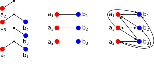
Figure 2: The leaf-colored tree $(T,\sigma)$ on the left explains the RBMG $G(T,\sigma)$ (middle) and the BMG $\mathaccent 382{G}(T,\sigma)$ (right). The colored graph $\mathaccent 382{G}(T,\sigma)$ is $\mathsf{R}$-thin. Thus, all leaves within an $\mathsf{R}$-class are trivially of the same color. However, in the RBMG we have $N(a_{2})=N(b_{3})=\emptyset$ but $a_{2}$ and $b_{3}$ are of different color. Note, by definition $a_{2}$ and $b_{3}$ are not within the same $\mathsf{S}$-class.

For an undirected colored graph $(G,\sigma)$, we denote by $G/\mathsf{S}$ the graph whose vertex set are exactly the $\mathsf{S}$-classes of $(G,\sigma)$, and two distinct classes $[x]$ and $[y]$ are connected by an edge in $G/\mathsf{S}$ if there is an $x^{\prime}\in[x]$ and $y^{\prime}\in[y]$ with $x^{\prime}y^{\prime}\in E(G)$. Moreover, since the vertices within each $\mathsf{S}$-class have the same color, the map $\sigma_{/\mathsf{S}}\colon V(G/\mathsf{S})\to S$ with $\sigma_{/\mathsf{S}}([x])=\sigma(x)$ is well-defined.

Lemma 5.

$(G/\mathsf{S},\sigma_{/\mathsf{S}})$ is $\mathsf{S}$-thin for every undirected colored graph $(G,\sigma)$. Moreover, $xy\in E(G)$ if and only if $[x][y]\in E(G/\mathsf{S})$. Thus, $G$ is connected if and only if $G/\mathsf{S}$ is connected.

The map $\gamma_{\mathsf{S}}\colon V(G)\to V(G/\mathsf{S}):x\mapsto[x]$ collapses all elements of an $\mathsf{S}$-thin class in $(G,\sigma)$ to a single node in $(G_{/\mathsf{S}},\sigma_{/\mathsf{S}})$. Hence, the $\gamma_{\mathsf{S}}$-image of a connected component of $(G,\sigma)$ is a connected component in $(G_{/\mathsf{S}},\sigma_{/\mathsf{S}})$. Conversely, the pre-image of a connected component of $(G_{/\mathsf{S}},\sigma_{/\mathsf{S}})$ that contains an edge is a single connected component of $(G,\sigma)$. Furthermore, $(G_{/\mathsf{S}},\sigma_{/\mathsf{S}})$ contains at most one isolated vertex of each color $r\in S$. If it exists, then its pre-image is the set of all isolated vertices of color $r$ in $(G,\sigma)$; otherwise $(G,\sigma)$ has no isolated vertex of color $r$. Surprisingly, it suffices to characterize the $\mathsf{S}$-thin RBMGs:

Lemma 7.

$(G,\sigma)$ is an RBMG if and only if $(G/\mathsf{S},\sigma_{/\mathsf{S}})$ is an RBMG. Moreover, every RBMG $(G,\sigma)$ is explained by a tree $(\widehat{T},\sigma)$ in which any two vertices $x,x^{\prime}\in[x]$ of each $\mathsf{S}$-classes $[x]$ of $(G,\sigma)$ have the same parent.

Lemma 7 is illustrated in Fig. 3, where $a_{2}$ and $a_{4}$ belong to the same $\mathsf{S}$-thin class $[a_{2}]$. However, in the tree representation on the l.h.s., $a_{2}$ and $a_{4}$ are attached to different parents. Substituting the edge $\mathsf{par}(a_{4})a_{4}$ by $\mathsf{par}(a_{2})a_{4}$ and suppressing the vertex $\mathsf{par}(a_{4})$, which now has degree $2$, yields a tree $(\hat{T},\sigma)$ with $\mathsf{par}(a_{2})=\mathsf{par}(a_{4})$ that still explains $(G,\sigma)$. Next, we can remove the edges $\mathsf{par}(a_{2})a_{2}$ and $\mathsf{par}(a_{2})a_{4}$ as well as the leaves $a_{2}$ and $a_{4}$ from $(\hat{T},\sigma)$ and add the edge $\mathsf{par}(a_{2})[a_{2}]$. Finally, we replace any vertex $y\neq a_{2},a_{4}$ by $[y]$ and set $\sigma(x)=\sigma_{/\mathsf{S}}([x])$ for all $x\in V(\hat{T})$. The resulting tree explains the $\mathsf{S}$-thin RBMG $(G_{/\mathsf{S}},\sigma_{/\mathsf{S}})$.

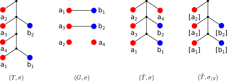
Figure 3: The leaf-colored tree $(T,\sigma)$ on the left explains the RBMG $(G,\sigma)$. Here, $a_{2},a_{4}\in[a_{2}]$ but they do not have the same parent in $T$. The tree $(\hat{T},\sigma)$ is obtained from $(T,\sigma)$ by re-attaching the leaf $a_{4}$ to $\mathsf{par}(a_{2})$ and suppressing the 2-degree vertex $\mathsf{par}(a_{4})$. The resulting tree still explains $(G,\sigma)$ and $a_{2}$ and $a_{4}$ are now siblings. Retaining only one representative of each $\mathsf{S}$-class finally gives the tree $(\tilde{T},\sigma_{/S})$ on the right that explains the $\mathsf{S}$-thin graph $(G_{/S},\sigma_{/S})$.

5 Connected Components

This section aims at simplifying the problem of finding a characterization for RBMGs by showing that an undirected colored graph is an RBMG if and only if each of its connected components is an RBMG (cf. Theorem 3) and at least one of them contains all colors. This, in turn, reduces the problem to connected graphs. This is a non-trivial observation since BMGs are not hereditary. Hence, we cannot expect RBMGs to be hereditary, either. They do satisfy a somewhat weaker property, however:

Lemma 9.

Let $(G,\sigma)$ be an RBMG with vertex set $L$ explained by $(T,\sigma)$ and let $(T_{|L^{\prime}},\sigma_{|L^{\prime}})$ be the restriction of $(T,\sigma)$ to $L^{\prime}\subseteq L$. Then the induced subgraph $(G,\sigma)[L^{\prime}]\coloneqq(G[L^{\prime}],\sigma_{|L^{\prime}})$ of $(G,\sigma)$ is a (not necessarily induced) subgraph of $G(T_{|L^{\prime}},\sigma_{|L^{\prime}})$.

Lemma 9 provides a starting point to show that the connected components of an RBMG are again RBMGs that can be explained by corresponding restrictions of a leaf-colored tree:

Theorem 2.

Let $(G^{*},\sigma^{*})$ with vertex set $L^{*}$ be a connected component of some RBMG $(G,\sigma)$ and let $(T,\sigma)$ be a leaf-colored tree explaining $(G,\sigma)$. Then, $(G^{*},\sigma^{*})$ is again an RBMG and is explained by the restriction $(T_{|L^{*}},\sigma_{|L^{*}})$ of $(T,\sigma)$ to $L^{*}$.

It is worth noting that there is no similar result for BMGs.

Every connected component of an $n$-RBMG is therefore a $k$-RBMG possibly with a strictly smaller number $k$ of colors. Our aim in the remainder of this section is to show that the disjoint union of RBMGs is again an RBMG provided that one of these RBMGs contains all colors.

Let $(G,\sigma)$ be an undirected, vertex colored graph with vertex set $L$ and $|\sigma(L)|=n$. We denote the connected components of $(G,\sigma)$ by $(G_{i}^{n},\sigma_{i}^{n})$, $1\leq i\leq k$, with vertex sets $L_{i}^{n}$ if $\sigma(L_{i}^{n})=\sigma(L)$ and $(G_{j}^{<n},\sigma_{j}^{<n})$, $1\leq j\leq l$, with vertex sets $L_{j}^{<n}$ if $\sigma(L_{j}^{<n})\subsetneq\sigma(L)$. That is, the upper index distinguishes components with all colors present from those that contain only a proper subset. Suppose that each $(G_{i}^{n},\sigma_{i}^{n})$ and $(G_{j}^{<n},\sigma_{j}^{<n})$ is an RBMG. Then there are trees $(T_{i}^{n},\sigma_{i}^{n})$ and $(T_{j}^{<n},\sigma_{j}^{<n})$ explaining $(G_{i}^{n},\sigma_{i}^{n})$ and $(G_{j}^{<n},\sigma_{j}^{<n})$, respectively. The roots of these trees are $u_{i}$ and $v_{j}$, respectively. We construct a tree $(T_{G}^{*},\sigma)$ with leaf set $L$ in two steps:

• Let $(T^{\prime},\sigma^{n})$ be the tree obtained by attaching the trees $(T_{i}^{n},\sigma_{i}^{n})$ with their roots $u_{i}$ to a common root $\rho^{\prime}$.

• First, construct a path $P=v_{1}v_{2}\dots v_{l-1}v_{l}\rho^{\prime}$, where $\rho^{\prime}$ is omitted whenever $T^{\prime}$ is empty. Now attach the trees $(T_{j}^{<n},\sigma_{j}^{<n})$, $1\leq j\leq l$, to $P$ by identifying the root of each $T_{j}^{<n}$ with the vertex $v_{j}$ in $P$. Finally, if $(T^{\prime},\sigma^{n})$ exists, attach it to $P$ by identifying the root of $T^{\prime}$ with the vertex $\rho^{\prime}$ in $P$. The coloring of $L$ is the one given for $(G,\sigma)$.

This construction is illustrated in Fig. 4 for $n\geq 2$. For $n=1$, the resulting tree is simply the star tree on $L$.

Figure 4: Shown is a tree $(T^{*}_{G},\sigma)$ that explains the graph $(G,\sigma)=\bigcup_{1\leq i\leq k}G((T_{i}^{n},\sigma_{i}^{n}))\cup\bigcup_{1\leq j\leq l}G((T_{j}^{<n},\sigma_{j}^{<n}))$ such that each of the subtrees $(T_{i}^{n},\sigma_{i}^{n})$ and $(T_{j}^{<n},\sigma_{j}^{<n})$ induces one connected component of $(G,\sigma)$. The subtree $(T_{i}^{n},\sigma_{i}^{n})$ explains the $n$-colored connected component $(G_{i}^{n},\sigma_{i}^{n})$ of $(G,\sigma)$. Each connected component $(G_{j}^{<n},\sigma_{j}^{<n})$ that does not contain all colors of $S$, is explained by a subtree $(T_{j}^{<n},\sigma_{j}^{<n})$. Any $n$-RBMG $(G,\sigma)$ can be explained by a tree of such form (cf. Lemma 16). See Fig. 5 for an explicit example of such a tree $(T^{*}_{G},\sigma)$.

We then proceed by demonstrating that it suffices to consider trees of the form $(T^{*}_{G},\sigma)$. The key result, Lemma 16 in the technical part, shows that an undirected vertex colored graph $(G,\sigma)$ whose connected components are RBMGs can be explained by $(T^{*}_{G},\sigma)$ provided $(G,\sigma)$ contains a connected component in which all colors are represented. It is not hard to check that these conditions are also necessary.

Theorem 3.

An undirected leaf-colored graph $(G,\sigma)$ is an RBMG if and only if each of its connected components is an RBMG and at least one connected component contains all colors.

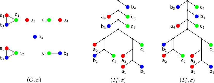
Figure 5: The trees $(T_{1}^{*},\sigma)$ and $(T_{2}^{*},\sigma)$ both explain the 3-RBMG $(G,\sigma)$ with five connected components and are of the form $(T^{*}_{G},\sigma)$.

The existence of an connected component using all colors is crucial for the statement above. Consider, for instance, an edge-less graph on two vertices, where both vertices have different color. Each of the two connected components is clearly an RBMG, however, one easily checks that their disjoint union is not.

Corollary 4.

Every RBMG can be explained by a tree of the form $(T^{*}_{G},\sigma)$.

By Theorem 3, it suffices to consider each connected component of an RBMG separately. In the following section, hence, we will consider the characterization of connected RBMGs.

6 Three Classes of Connected 3-RBMGs

Reciprocal best match graphs on two colors convey very little structural information. Their connected components are either single vertices or complete bipartite graphs (Geiß et al., 2019b, Cor. 6), which reduce to a $K_{2}$ with two distinctly colored vertices under $\mathsf{S}$-thinness. Connected 3-RBMGs, in contrast, can be quite complex. As we shall see, they fall into three distinct classes which correspond to trees with different shapes. In the next section we will make use of 3-RBMGs to characterize general $n$-RBMGs.

Our starting point are three types of leaf-colored trees on three colors:

Definition 11.

Let $(T,\sigma)$ be a 3-colored tree with color set $S=\{r,s,t\}$. The tree $(T,\sigma)$ is of

Type (I),

if there exists $v\in\mathsf{child}(\rho_{T})$ such that $|\sigma(L(T(v)))|=2$ and $\mathsf{child}(\rho_{T})\setminus\{v\}\subsetneq L$.

Type (II),

if there exists $v_{1},v_{2}\in\mathsf{child}(\rho_{T})$ such that $|\sigma(L(T(v_{1})))|=|\sigma(L(T(v_{2})))|=2$, $\sigma(L(T(v_{1})))\neq\sigma(L(T(v_{2})))$ and $\mathsf{child}(\rho_{T})\setminus\{v_{1},v_{2}\}\subsetneq L$,

Type (III),

if there exists $v_{1},v_{2},v_{3}\in\mathsf{child}(\rho_{T})$ such that $\sigma(L(T(v_{1})))=\{r,s\}$, $\sigma(L(T(v_{2})))=\{r,t\}$, $\sigma(L(T(v_{3})))=\{s,t\}$, and $\mathsf{child}(\rho_{T})\setminus\{v_{1},v_{2},v_{3}\}\subsetneq L$.

Fig. 6 illustrates these three tree types.

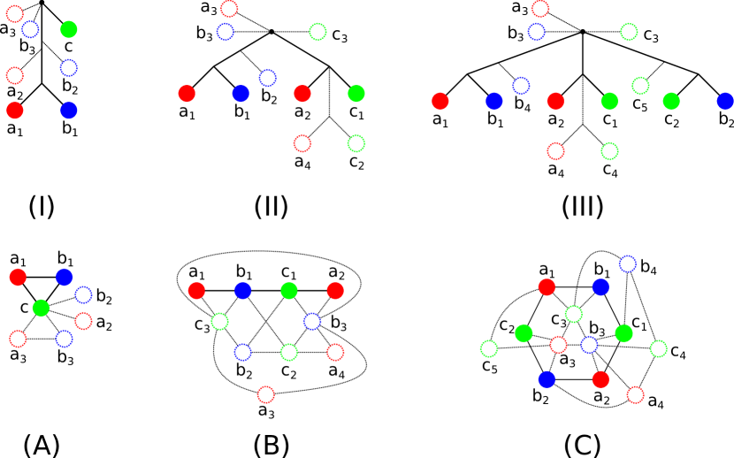
Figure 6: The three categories of three-colored connected 3-RBMGs are shown on the bottom: (A) Contains a $K_{3}$ on three colors but no induced $C_{n}$, $n\geq 5$ or $P_{4}$, (B) contains an induced $P_{4}$, whose endpoints have the same color, but no induced $C_{n}$ with $n\geq 5$, (C) contains a $C_{6}$ of the form $(r,s,t,r,s,t)$. The corresponding tree Types (I), (II), and (III) are shown on top. Solid lines represent edges and vertices that must necessarily be contained in the graph, dashed elements may be missing.

Correspondingly, we distinguish three classes of 3-colored graphs:

Definition 13.

An undirected, connected graph $(G,\sigma)$ on three colors is of

Type (A)

if $(G,\sigma)$ contains a $K_{3}$ on three colors but no induced $P_{4}$, and thus also no induced $C_{n}$, $n\geq 5$.

Type (B)

if $(G,\sigma)$ contains an induced $P_{4}$ on three colors whose endpoints have the same color, but no no induced $C_{n}$ for $n\geq 5$.

Type (C)

if $(G,\sigma)$ contains an induced $C_{6}$ along which the three colors appear twice in the same permutation, i.e., $(r,s,t,r,s,t)$.

The main result of this section is that each tree class explains the RBMGs belonging to one of the classes of colored graphs. More precisely:

Theorem 4.

Let $(G,\sigma)$ be an $\mathsf{S}$-thin connected 3-RBMG. Then $(G,\sigma)$ is either of Type (A), (B), or (C). An RBMG of Type (A), (B), and (C), resp., can be explained by a tree of Type (I), (II), and (III), respectively.

An undirected, colored graph $(G,\sigma)$ contains an induced $K_{3}$, $P_{4}$, or $C_{6}$, respectively, if and only if $(G/\mathsf{S},\sigma/\mathsf{S})$ contains an induced $K_{3}$, $P_{4}$, or $C_{6}$, resp., on the same colors (cf. Lemma 5). An immediate consequence of this fact is

Theorem 5.

A connected (not necessarily $\mathsf{S}$-thin) 3-RBMG $(G,\sigma)$ is either of Type (A), (B), or (C).

As a further consequence of Theorem 4 and the well-known properties of cographs (Corneil et al., 1981) we obtain

Observation 3.

Let $(G,\sigma)$ be a connected, $\mathsf{S}$-thin 3-RBMG. Then it is of Type (A) if and only if it is a cograph.

This observation is of practical interest because orthology relations are necessarily cographs (Hellmuth et al., 2013). Hence, 3-RBMGs cannot perfectly reflect orthology unless they are of Type (A).

So-called hub-vertices play a key role for the characterization of Type (A) 3-RBMGs:

Definition 14.

Let $G=(V,E)$ be an undirected graph. A vertex $x\in V(G)$ such that $N(x)=V\setminus\{x\}$ is a hub-vertex.

Lemma 22.

A properly vertex colored, connected, $\mathsf{S}$-thin graph $(G,\sigma)$ on three colors with vertex set $L$ is a 3-RBMG of Type (A) if and only if $G\notin\mathscr{P}_{3}$ and it satisfies the following conditions:

1. $G$ contains a hub-vertex $x$, i.e., $N(x)=V(G)\setminus\{x\}$

2. $|N(y)|<3$ for every $y\in V(G)\setminus\{x\}$.

We proceed by characterizing Type (B) and (C) 3-RBMGs. To this end, we first introduce B-like and C-like graphs $(G,\sigma)$:

Definition 15.

Let $(G,\sigma)$ be an undirected, connected, properly colored, $\mathsf{S}$-thin graph with vertex set $L$ and color set $\sigma(L)=\{r,s,t\}$, and assume that $(G,\sigma)$ contains the induced path $P\coloneqq\langle\hat{x}_{1}\hat{y}\hat{z}\hat{x}_{2}\rangle$ with $\sigma(\hat{x}_{1})=\sigma(\hat{x}_{2})=r$, $\sigma(\hat{y})=s$, and $\sigma(\hat{z})=t$. Then $(G,\sigma)$ is B-like w.r.t. $P$ if (i) $N_{r}(\hat{y})\cap N_{r}(\hat{z})=\emptyset$, and (ii) $G$ does not contain an induced cycle $C_{n}$, $n\geq 5$.

An example is given in Fig. 7.

Figure 7: The graph $(G,\sigma)$ is a 3-RBMG since it is explained by $(T,\sigma)$. Moreover, $(G,\sigma)$ does not contain an induced $C_{n}$, $n\geq 5$ but induced $P_{4}$s, thus it is of Type (B). It is easy to see that $(G,\sigma)$ is B-like w.r.t. $\langle x_{1}yzx_{2}\rangle$. However, $(G,\sigma)$ is not B-like w.r.t. $\langle x_{1}z^{\prime}y^{\prime}x_{2}\rangle$, since $x^{\prime}\in N_{r}(y^{\prime})\cap N_{r}(z^{\prime})$.

For a $3$-colored, $\mathsf{S}$-thin graph $(G,\sigma)$ that is B-like w.r.t. the induced path $P\coloneqq\langle\hat{x}_{1}\hat{y}\hat{z}\hat{x}_{2}\rangle$ we define the following subsets of vertices:

$$L_{t,s}^{P}\coloneqq \{y\mid\langle xy\hat{z}\rangle\in\mathscr{P}_{3}\text{ for any }x\in N_{r}(y)\}$$

$$L_{t,r}^{P}\coloneqq \{x\mid N_{r}(y)=\{x\}\text{ and }\langle xy\hat{z}\rangle\in\mathscr{P}_{3}\}\cup$$

$$\{x\mid x\in L[r],\,N_{s}(x)=\emptyset,\,L[s]\setminus L_{t,s}^{P}\neq\emptyset\}$$

$$L_{s,t}^{P}\coloneqq \{z\mid\langle xz\hat{y}\rangle\in\mathscr{P}_{3}\text{ for any }x\in N_{r}(z)\}$$

$$L_{s,r}^{P}\coloneqq \{x\mid N_{r}(z)=\{x\}\text{ and }xz\hat{y}\in\mathscr{P}_{3}\}\cup$$

$$\{x\mid x\in L[r],N_{t}(x)=\emptyset,L[t]\setminus L_{s,t}^{P}\neq\emptyset\}$$

The first subscripts $t$ and $s$ refer to the color of the vertices $\hat{z}$ and $\hat{y}$, respectively, that “anchor” the $P_{3}$s within the defining path $P$. The second index identifies the color of the vertices in the respective set, since by definition we have $L_{t,s}^{P}\subseteq L[s]$, $L_{t,r}^{P}\subseteq L[r]$, $L_{s,t}^{P}\subseteq L[t]$ and $L_{s,r}^{P}\subseteq L[r]$. Furthermore, we set

$$L_{t}^{P}\coloneqq L_{t,s}^{P}\cup L_{t,r}^{P}$$

$$L_{s}^{P}\coloneqq L_{s,t}^{P}\cup L_{s,r}^{P}$$

$$L_{*}^{P}\coloneqq L\setminus(L_{t}^{P}\cup L_{s}^{P}).$$

By definition, $L_{s,r}^{P}=L_{s}^{P}\cap L[r]$, $L_{t,r}^{P}=L_{t}^{P}\cap L[r]$, $L_{s,t}^{P}=L_{s}^{P}\cap L[t]$, and $L_{t,s}^{P}=L_{t}^{P}\cap L[s]$. For simplicity we will often write $L_{*}^{P}[i]\coloneqq L_{*}^{P}\cap L[i]$ for $i\in\{s,t\}$.

The construction of Type (B) 3-RBMGs can be extended to a similar one of Type (C) 3-RBMGs.

Definition 16.

Let $(G,\sigma)$ be an undirected, connected, properly colored, $\mathsf{S}$-thin graph. Moreover, assume that $(G,\sigma)$ contains the hexagon $H\coloneqq\langle\hat{x}_{1}\hat{y}_{1}\hat{z}_{1}\hat{x}_{2}\hat{y}_{2}\hat{z}_{2}\rangle$ such that $\sigma(\hat{x}_{1})=\sigma(\hat{x}_{2})=r$, $\sigma(\hat{y}_{1})=\sigma(\hat{y}_{2})=s$, and $\sigma(\hat{z}_{1})=\sigma(\hat{z}_{2})=t$. Then, $(G,\sigma)$ is C-like w.r.t. $H$ if there is a vertex $v\in\{\hat{x}_{1},\hat{y}_{1},\hat{z}_{1},\hat{x}_{2},\hat{y}_{2},\hat{z}_{2}\}$ such that $|N_{c}(v)|>1$ for some color $c\neq\sigma(v)$. Suppose that $(G,\sigma)$ is C-like w.r.t. $H=\langle\hat{x}_{1}\hat{y}_{1}\hat{z}_{1}\hat{x}_{2}\hat{y}_{2}\hat{z}_{2}\rangle$ and assume w.l.o.g. that $v=\hat{x}_{1}$ and $c=t$, i.e., $|N_{t}(\hat{x}_{1})|>1$. Then we define the following sets:

$$L_{t}^{H} \coloneqq\{x\mid\langle x\hat{z}_{2}\hat{y}_{2}\rangle\in\mathscr{P}_{3}\}\cup\{y\mid\langle y\hat{z}_{1}\hat{x}_{2}\rangle\in\mathscr{P}_{3}\}$$

$$L_{s}^{H} \coloneqq\{x\mid\langle x\hat{y}_{2}\hat{z}_{2}\rangle\in\mathscr{P}_{3}\}\cup\{z\mid\langle z\hat{y}_{1}\hat{x}_{1}\in\rangle\mathscr{P}_{3}\}$$

$$L_{r}^{H} \coloneqq\{y\mid\langle y\hat{x}_{2}\hat{z}_{1}\rangle\in\mathscr{P}_{3}\}\cup\{z\mid\langle z\hat{x}_{1}\hat{y}_{1}\rangle\in\mathscr{P}_{3}\}$$

$$L_{*}^{H} \coloneqq V(G)\setminus(L_{r}^{H}\cup L_{s}^{H}\cup L_{t}^{H}).$$

The main result of this section is the following, rather technical, result, which provides a complete characterization of 3-colored RBMGs.

Theorem 6.

Let $(G,\sigma)$ be an undirected, connected, $\mathsf{S}$-thin, and properly 3-colored graph with color set $S=\{r,s,t\}$ and let $x\in L[r]$, $y\in L[s]$ and $z\in L[t]$. Then $(G,\sigma)$ is a 3-RBMG if and only if one of the following is true:

1. Conditions (A1) and (A2) are satisfied, or

2. Conditions (B1) to (B3.b) are satisfied, after possible permutation of the colors, where:

   (B1)

   $(G,\sigma)$ is B-like w.r.t. $P=\langle\hat{x}_{1}\hat{y}\hat{z}\hat{x}_{2}\rangle$ for some $\hat{x}_{1},\hat{x}_{2}\in L[r]$, $\hat{y}\in L[s]$, $\hat{z}\in L[t]$,

   (B2.a)

   If $x\in L_{*}^{P}$, then $N(x)=L_{*}^{P}\setminus\{x\}$,

   (B2.b)

   If $x\in L_{t}^{P}$, then $N_{s}(x)\subset L_{t}^{P}$ and $|N_{s}(x)|\leq 1$, and $N_{t}(x)=L_{*}^{P}[t]$,

   (B2.c)

   If $x\in L_{s}^{P}$, then $N_{t}(x)\subset L_{s}^{P}$ and $|N_{t}(x)|\leq 1$, and $N_{s}(x)=L_{*}^{P}[s]$

   (B3.a)

   If $y\in L_{*}^{P}$, then $N(y)=L_{s}^{P}\cup(L_{*}^{P}\setminus\{y\})$,

   (B3.b)

   If $y\in L_{t}^{P}$, then $N_{r}(y)\subset L_{t}^{P}$ and $|N_{r}(y)|\leq 1$, and $N_{t}(y)=L[t]$,

   or

3. $(G,\sigma)$ is either a hexagon or $|L|>6$ and, up to permutation of colors, the following conditions are satisfied:

   (C1)

   $(G,\sigma)$ is C-like w.r.t. the hexagon $H=\langle\hat{x}_{1}\hat{y}_{1}\hat{z}_{1}\hat{x}_{2}\hat{y}_{2}\hat{z}_{2}\rangle$ for some $\hat{x}_{i}\in L[r]$, $\hat{y}_{i}\in L[s]$, $\hat{z}_{i}\in L[t]$ with $|N_{t}(\hat{x}_{1})|>1$,

   (C2.a)

   If $x\in L_{*}^{H}$, then $N(x)=L_{r}^{H}\cup(L_{*}^{H}\setminus\{x\})$,

   (C2.b)

   If $x\in L_{t}^{H}$, then $N_{s}(x)\subset L_{t}^{H}$ and $|N_{s}(x)|\leq 1$, and $N_{t}(x)=L_{*}^{H}[t]\cup L_{r}^{H}[t]$,

   (C2.c)

   If $x\in L_{s}^{H}$, then $N_{t}(x)\subset L_{s}^{H}$ and $|N_{t}(x)|\leq 1$, and $N_{s}(x)=L_{*}^{H}[s]\cup L_{r}^{H}[s]$

   (C3.a)

   If $y\in L_{*}^{H}$, then $N(y)=L_{s}^{H}\cup(L_{*}^{H}\setminus\{y\})$,

   (C3.b)

   If $y\in L_{t}^{H}$, then $N_{r}(y)\subset L_{t}^{H}$ and $|N_{r}(y)|\leq 1$, and $N_{t}(y)=L_{*}^{H}[t]\cup L_{s}^{H}[t]$,

   (C3.c)

   If $y\in L_{r}^{H}$, then $N_{t}(y)\subset L_{r}^{H}$ and $|N_{t}(y)|\leq 1$, and $N_{r}(y)=L_{*}^{H}[r]\cup L_{s}^{H}[r]$.

Remark 1.

As a consequence of Lemma 5, every (not necessarily $\mathsf{S}$-thin) Type (B) 3-RBMG $(G,\sigma)$ contains an induced path $\langle xyzx^{\prime}\rangle$ with $\sigma(x)=\sigma(x^{\prime})=r$, $\sigma(y)=s$, and $\sigma(z)=t$ for distinct colors $r,s,t$ such that $N_{r}(y)\cap N_{r}(z)=\emptyset$. Similarly, every Type (C) 3-RBMG $(G,\sigma)$ contains a hexagon $\langle xyzx^{\prime}y^{\prime}z^{\prime}\rangle$ with $\sigma(x)=\sigma(x^{\prime})=r$, $\sigma(y)=\sigma(y^{\prime})=s$, and $\sigma(z)=\sigma(z^{\prime})=t$ for distinct colors $r,s,t$ such that $|N_{c}(v)|>1$ for some $v\in\{x,x^{\prime},y,y^{\prime},z,z^{\prime}\}$ and $c\neq\sigma(v)$.

In the technical part we describe an algorithm that determines whether a given properly 3-colored connected graph $(G,\sigma)$ is a 3-RBMG and, in the positive case, returns a tree $(T,\sigma)$ that explains $(G,\sigma)$ in $O(mn^{2}+m^{\prime})$ time, where $n=|V(G/\mathsf{S})|$, $m=|E(G/\mathsf{S})|$ and $m^{\prime}=|E(G)|$ (cf. Algorithm 1, Lemmas 31 and 30).

In addition, we provide in Section E in the technical part results about the structure of induced $P_{4}$s in RBMGs. In particular, those $P_{4}$s can be classified as so-called good, bad, and ugly quartets and the sets $L_{t}^{P}$, $L_{s}^{P}$, and $L_{*}^{P}$ can be determined by good quartets and are independent of the choice of the respective good quartet. As shown by Geiß et al. (2019a), good quartets also play an important role for the detection of false positive and false negative orthology assignments.

7 Characterization of $n$-RBMGs

The first part of this section is dedicated to the characterization of $n$-RBMGs by combining the sets of least resolved trees for the induced 3-RBMGs for any triplet of colors. It remains, however, an open question if the problem of recognizing $n$-RBMGs can be solved in polynomial time. Because of the importance of cographs in best-match-based orthology assignment methods, we investigate co-RBMGs, i.e., $n$-RBMGs that are cographs, in more detail and provide a characterization of this subclass.

7.1 The General Case: Combination of 3-RBMGs

It will be convenient in the following to use the simplified notation

Definition 18.

$(G_{rst},\sigma_{rst})\coloneqq(G[L[r]\cup L[s]\cup L[t]],\sigma_{|L[r]\cup L[s]\cup L[t]})$ and $(T_{rst},\sigma_{rst})\coloneqq(T_{|L[r]\cup L[s]\cup L[t]},\sigma_{|L[r]\cup L[s]\cup L[t]})$ for any three colors $r,s,t\in S$.

The restriction of a BMG $\mathaccent 382{G}(T,\sigma)$ to a subset $S^{\prime}\subset S$ of colors is an induced subgraph of $\mathaccent 382{G}(T,\sigma)$ explained by the restriction of $(T,\sigma)$ to the leaves with colors in $S^{\prime}$, an thus again a BMG (Geiß et al., 2019b, Observation 1). Since $G(T,\sigma)$ is the symmetric part of $\mathaccent 382{G}(T,\sigma)$, it inherits this property. In particular, we have

Observation 6.

If $(G,\sigma)$ is an $n$-RBMG, $n\geq 3$ explained by $(T,\sigma)$, then for any three colors $r,s,t\in S$, the restricted tree $(T_{rst},\sigma_{rst})$ explains $(G_{rst},\sigma_{rst})$, and $(G_{rst},\sigma_{rst})$ is an induced subgraph of $(G,\sigma)$.

The key idea of characterizing $n$-RBMGs is to combine the information contained in their 3-colored induced subgraphs $(G_{rst},\sigma_{rst})$. Observation 6 plays a major role in this context. It shows that $(G_{rst},\sigma_{rst})$ is an induced subgraph of an $n$-RBMG and it is always a 3-RBMG that is explained by $(T_{rst},\sigma_{rst})$. Unfortunately, the converse of Observation 6 is in general not true. Fig. 8 shows a 4-colored graph that is not a 4-RBMG while each of the four subgraphs induced by a triplet of colors is a 3-RBMG. We can, however, rephrase Observation 6 in the following way:

Observation 7.

Let $(G,\sigma)$ be an $n$-RBMG for some $n\geq 3$. Then, $(T,\sigma)$ explains $(G,\sigma)$ if and only if $(T_{rst},\sigma_{rst})$ explains $(G_{rst},\sigma_{rst})$ for all triplets of colors $r,s,t\in S$.

Figure 8: The 4-colored graph $(G,\sigma)$ in (A) with color set $S=\{A,B,C,D\}$ is not an RBMG. All four subgraphs induced by three of the four colors, however, are (not necessarily connected) 3-RBMGs. These are explained by the unique least resolved trees in (B). Because of the uniqueness of the least resolved trees on three colors, the tree explaining $(G,\sigma)$ must display these four trees. The tree $(T,\sigma)$ in Panel (C) is the least resolved supertree of $\mathcal{P}\coloneqq\bigcup_{r,s,t\in S}T_{rst}$. However, $(T,\sigma)$ does not explain $(G,\sigma)$ since the edge $b_{2}c$ is not contained in $G(T,\sigma)$. Clearly, there exists no refinement $(T^{\prime},\sigma)$ of $(T,\sigma)$ such that $b_{2}c\in E(G(T^{\prime},\sigma))$ and therefore $(G,\sigma)$ is not an RBMG.

Definition 19.

Let $(G,\sigma)$ be an $n$-RBMG. Then the tree set of $(G,\sigma)$ is the set

$$\mathcal{T}(G,\sigma)\coloneqq\{(T,\sigma)\mid\color[rgb]{0,0,0}(T,\sigma)\text{ is least resolved and }G(T,\sigma)=(G,\sigma)\}$$

of all leaf-colored trees explaining $(G,\sigma)$. Furthermore, we write $\mathcal{T}_{rst}(G,\sigma)$ for the set of all least resolved trees explaining the induced subgraphs $(G_{rst},\sigma_{rst})$.

It is tempting to conjecture that the existence of a supertree for the tree set $\mathcal{P}\coloneqq\{T\in\mathcal{T}_{rst}(G_{rst},\sigma_{rst}),\,r,s,t\in S\}$ is sufficient for $(G,\sigma)$ to be an $n$-RBMG. However, this is not the case as shown by the counterexample in Fig. 8.

Theorem 7.

A (not necessarily connected) undirected colored graph $(G,\sigma)$ is an $n$-RBMG if and only if (i) all induced subgraphs $(G_{rst},\sigma_{rst})$ on three colors are 3-RBMGs and (ii) there exists a supertree $(T,\sigma)$ of the tree set $\mathcal{P}\coloneqq\{T\in\mathcal{T}_{rst}(G,\sigma)\mid r,s,t\in S\}$, such that $G(T,\sigma)=(G,\sigma)$.

Whether the recognition problem of $n$-RBMGs is NP-hard or not may strongly depend on the number of least resolved trees for a given 3-colored induced subgraph. However, even if this number is polynomial bounded in the input size (e.g. number of vertices), the number of possible (least resolved) trees that explain a given $n$-RBMG, may grow exponentially. In particular, since the order of the inner nodes in the 2-colored subtrees of Type (I), (II), and (III) trees is in general arbitrary, determining the number of least resolved trees seems to be far from trivial. We therefore leave it as an open problem.

7.2 Characterization of $n$-RBMGs that are cographs

Probably the most important application of reciprocal best matches is orthology detection. Since orthology relations are cographs (Hellmuth et al., 2013), it is of particular interest to characterize RBMGs of this type. Since cographs are hereditary (see e.g. (Sumner, 1974) where they are called Hereditary Dacey graphs), one expects their 3-colored restrictions to be of Type (A). The next theorem shows that this intuition is essentially correct. It is based on the following observation about cographs:

Observation 8.

Any undirected colored graph $(G,\sigma)$ is a cograph if and only if the corresponding $\mathsf{S}$-thin graph $(G/\mathsf{S},\sigma_{/\mathsf{S}})$ is a cograph.

Theorem 8.

Let $(G,\sigma)$ be an $n$-RBMG with $n\geq 3$, and denote by $(G^{\prime}_{rst},\sigma^{\prime}_{rst})\coloneqq(G_{rst}/S,\sigma_{rst}/S)$ the $\mathsf{S}$-thin version of the 3-RBMG that is obtained by restricting $(G,\sigma)$ to the colors $r$, $s$, and $t$. Then $(G,\sigma)$ is a cograph if and only if every 3-colored connected component of $(G^{\prime}_{rst},\sigma^{\prime}_{rst})$ is a 3-RBMG of Type (A) for all triples of distinct colors $r,s,t$.

Remark 2.

Theorem 8 has been stated for $\mathsf{S}$-thin induced 3-RBMGs only. However, as a consequence of Lemma 5, it extends to general RBMGs, i.e., an $n$-RBMG $(G,\sigma)$ is a cograph if and only if every 3-colored connected component of $(G_{rst},\sigma_{rst})$ is a Type (A) 3-RBMG for all triplets of distinct colors $r,s,t$.

7.3 Hierarchically Colored Cographs

Thm. 8 yields a polynomial time algorithm for recognizing $n$-RBMGs that are cographs. It is not helpful, however, for the reconstruction of a tree $(T,\sigma)$ that explains such a graph. Below, we derive an alternative characterization in terms of so-called hierarchically colored cographs (hc-cographs). As we shall see, the cotrees of hc-cographs explain a given $n$-RBMG and can be constructed in polynomial time.

Definition 20.

A graph that is both a cograph and an RBMG is a co-RBMG.

Cographs are constructed using joins and disjoint unions. We extend these graph operations to vertex colored graphs.

Definition 21.

Let $(H_{1},\sigma_{H_{1}})$ and $(H_{2},\sigma_{H_{2}})$ be two vertex-disjoint colored graphs. Then $(H_{1},\sigma_{H_{1}})\operatorname{\triangledown}(H_{2},\sigma_{H_{2}})\coloneqq(H_{1}\operatorname{\triangledown}H_{2},\sigma)$ and $(H_{1},\sigma_{H_{1}})\mathbin{\mathchoice{\leavevmode\vtop{\halign{\hfil$\m@th\displaystyle#$\hfil\cr\cup\cr\cdot\crcr}}}{\leavevmode\vtop{\halign{\hfil$\m@th\textstyle#$\hfil\cr\cup\cr\cdot\crcr}}}{\leavevmode\vtop{\halign{\hfil$\m@th\scriptstyle#$\hfil\cr\cup\cr\cdot\crcr}}}{\leavevmode\vtop{\halign{\hfil$\m@th\scriptscriptstyle#$\hfil\cr\cup\cr\cdot\crcr}}}}(H_{2},\sigma_{H_{2}})\coloneqq(H_{1}\mathbin{\mathchoice{\leavevmode\vtop{\halign{\hfil$\m@th\displaystyle#$\hfil\cr\cup\cr\cdot\crcr}}}{\leavevmode\vtop{\halign{\hfil$\m@th\textstyle#$\hfil\cr\cup\cr\cdot\crcr}}}{\leavevmode\vtop{\halign{\hfil$\m@th\scriptstyle#$\hfil\cr\cup\cr\cdot\crcr}}}{\leavevmode\vtop{\halign{\hfil$\m@th\scriptscriptstyle#$\hfil\cr\cup\cr\cdot\crcr}}}}H_{2},\sigma)$ denotes their join and union, respectively, where $\sigma(x)=\sigma_{H_{i}}(x)$ for every $x\in V(H_{i})$, $i\in\{1,2\}$.

Definition 22.

An undirected colored graph $(G,\sigma)$ is a hierarchically colored cograph (hc-cograph) if

• $(G,\sigma)=(K_{1},\sigma)$, i.e., a colored vertex, or

• $(G,\sigma)=(H,\sigma_{H})\operatorname{\triangledown}(H^{\prime},\sigma_{H^{\prime}})$ and $\sigma(V(H))\cap\sigma(V(H^{\prime}))=\emptyset$, or

• $(G,\sigma)=(H,\sigma_{H})\mathbin{\mathchoice{\leavevmode\vtop{\halign{\hfil$\m@th\displaystyle#$\hfil\cr\cup\cr\cdot\crcr}}}{\leavevmode\vtop{\halign{\hfil$\m@th\textstyle#$\hfil\cr\cup\cr\cdot\crcr}}}{\leavevmode\vtop{\halign{\hfil$\m@th\scriptstyle#$\hfil\cr\cup\cr\cdot\crcr}}}{\leavevmode\vtop{\halign{\hfil$\m@th\scriptscriptstyle#$\hfil\cr\cup\cr\cdot\crcr}}}}(H^{\prime},\sigma_{H^{\prime}})$ and $\sigma(V(H))\cap\sigma(V(H^{\prime}))\in\{\sigma(V(H)),\sigma(V(H^{\prime}))\}$,

where both $(H,\sigma_{H})$ and $(H^{\prime},\sigma_{H^{\prime}})$ are hc-cographs. For the color-constraints (cc) in (K2) and (K3), we simply write (K2cc) and (K3cc), respectively.

Omitting the color-constraints reduces Def. 22 to Def. 4. Therefore we have

Observation 9.

If $(G,\sigma)$ is an hc-cograph, then $G$ is cograph.

The recursive construction of an hc-cograph $(G,\sigma)$ according to Def. 22 immediately produces a binary hc-cotree $T^{G}_{\emph{hc}}$ corresponding to $(G,\sigma)$. The construction is essentially the same as for the cotree of a cograph (cf. Corneil et al. (1981, Section 3)): Each of its inner vertices is labeled by $1$ for a $\operatorname{\triangledown}$ operation and $0$ for a disjoint union $\mathbin{\mathchoice{\leavevmode\vtop{\halign{\hfil$\m@th\displaystyle#$\hfil\cr\cup\cr\cdot\crcr}}}{\leavevmode\vtop{\halign{\hfil$\m@th\textstyle#$\hfil\cr\cup\cr\cdot\crcr}}}{\leavevmode\vtop{\halign{\hfil$\m@th\scriptstyle#$\hfil\cr\cup\cr\cdot\crcr}}}{\leavevmode\vtop{\halign{\hfil$\m@th\scriptscriptstyle#$\hfil\cr\cup\cr\cdot\crcr}}}}$, depending on whether (K2) or (K3) is used in the construction steps. We write $t:V^{0}(T^{G}_{\emph{hc}})\to\{0,1\}$ for the labeling of the inner vertices. The recursion terminates with a leaf of $T^{G}_{\emph{hc}}$ whenever a colored single-vertex graph, i.e., (K1) is reached. We therefore identify the leaves of $T^{G}_{\emph{hc}}$ with the vertices of $(G,\sigma)$. The binary hc-cograph $(T^{G}_{\emph{hc}},t,\sigma)$ with leaf coloring $\sigma$ and labeling $t$ at its inner vertices uniquely determines $(G,\sigma)$, i.e., $xy\in E(G)$ if and only if $t(\operatorname{lca}(x,y))=1$.

By construction, $(T^{G}_{\emph{hc}},t)$ is a not necessarily discriminating cotree for $G$. An example for different constructions of $(T^{G}_{\emph{hc}},t,\sigma)$ based on the particular hc-cograph representation of $(G,\sigma)$ is given in Fig. 9.

While the cograph property is hereditary, this is no longer true for hc-cographs, i.e., an hc-cograph may contain induced subgraphs that are not hc-cographs. As an example, consider the three single vertex graphs $(G_{i},\sigma_{i})$ with $V_{i}=\{i\}$ and colors $\sigma_{1}(1)=r$ and $\sigma_{2}(2)=\sigma_{3}(3)=s\neq r$. Then $(G,\sigma)=((G_{1},\sigma_{1})\operatorname{\triangledown}(G_{2},\sigma_{2}))\mathbin{\mathchoice{\leavevmode\vtop{\halign{\hfil$\m@th\displaystyle#$\hfil\cr\cup\cr\cdot\crcr}}}{\leavevmode\vtop{\halign{\hfil$\m@th\textstyle#$\hfil\cr\cup\cr\cdot\crcr}}}{\leavevmode\vtop{\halign{\hfil$\m@th\scriptstyle#$\hfil\cr\cup\cr\cdot\crcr}}}{\leavevmode\vtop{\halign{\hfil$\m@th\scriptscriptstyle#$\hfil\cr\cup\cr\cdot\crcr}}}}(G_{3},\sigma_{3})$ is an hc-cograph. However, the induced subgraph $(G,\sigma)[1,3]=(G_{1},\sigma_{1})\mathbin{\mathchoice{\leavevmode\vtop{\halign{\hfil$\m@th\displaystyle#$\hfil\cr\cup\cr\cdot\crcr}}}{\leavevmode\vtop{\halign{\hfil$\m@th\textstyle#$\hfil\cr\cup\cr\cdot\crcr}}}{\leavevmode\vtop{\halign{\hfil$\m@th\scriptstyle#$\hfil\cr\cup\cr\cdot\crcr}}}{\leavevmode\vtop{\halign{\hfil$\m@th\scriptscriptstyle#$\hfil\cr\cup\cr\cdot\crcr}}}}(G_{3},\sigma_{3})$ is not an hc-cograph, since $\sigma_{1}(V_{1})\cap\sigma_{3}(V_{3})=\emptyset$ and hence, $(G,\sigma)[1,3]$ does not satisfy Property (K3cc).

Both $\operatorname{\triangledown}$ and $\mathbin{\mathchoice{\leavevmode\vtop{\halign{\hfil$\m@th\displaystyle#$\hfil\cr\cup\cr\cdot\crcr}}}{\leavevmode\vtop{\halign{\hfil$\m@th\textstyle#$\hfil\cr\cup\cr\cdot\crcr}}}{\leavevmode\vtop{\halign{\hfil$\m@th\scriptstyle#$\hfil\cr\cup\cr\cdot\crcr}}}{\leavevmode\vtop{\halign{\hfil$\m@th\scriptscriptstyle#$\hfil\cr\cup\cr\cdot\crcr}}}}$ are commutative and associative operations on graphs. For a given cograph $G$, hence, alternative binary cotrees may exist that can be transformed into each other by applying the commutative or associative laws. This is no longer true for hc-cographs as a consequence of the color constraints. There are no restrictions on commutativity, i.e., if $(G,\sigma)$ can be obtained as the join $(H,\sigma_{H})\operatorname{\triangledown}(H^{\prime},\sigma_{H^{\prime}})$, equivalently we have $(G,\sigma)=(H^{\prime},\sigma_{H^{\prime}})\operatorname{\triangledown}(H,\sigma_{H})$. The same holds for the disjoint union $\mathbin{\mathchoice{\leavevmode\vtop{\halign{\hfil$\m@th\displaystyle#$\hfil\cr\cup\cr\cdot\crcr}}}{\leavevmode\vtop{\halign{\hfil$\m@th\textstyle#$\hfil\cr\cup\cr\cdot\crcr}}}{\leavevmode\vtop{\halign{\hfil$\m@th\scriptstyle#$\hfil\cr\cup\cr\cdot\crcr}}}{\leavevmode\vtop{\halign{\hfil$\m@th\scriptscriptstyle#$\hfil\cr\cup\cr\cdot\crcr}}}}$. If $(G,\sigma)$ is obtained as $(H,\sigma_{H})\operatorname{\triangledown}\big{(}(H^{\prime},\sigma_{H^{\prime}})\operatorname{\triangledown}(H^{\prime\prime},\sigma_{H^{\prime\prime}})\big{)}$, i.e., if $(H^{\prime},\sigma_{H^{\prime}})\operatorname{\triangledown}(H^{\prime\prime},\sigma_{H^{\prime\prime}})$ is also an hc-cograph, then the color sets of $H$, $H^{\prime}$, and $H^{\prime\prime}$ must be disjoint by Def. 22, and thus $(H,\sigma_{H})\operatorname{\triangledown}(H^{\prime},\sigma_{H^{\prime}})$ is also an hc-cograph. Condition K3cc, however, is not so well-behaved:

Example 1.

Consider the single vertex graphs $(G_{i},\sigma_{i})$ with vertex set $V_{i}=\{i\}$, $1\leq i\leq 4$ and colors $\sigma(i)=r$ if $i$ is odd and $\sigma(i)=s\neq r$ if $i$ is even. Consider the graph $G=G_{1}\mathbin{\mathchoice{\leavevmode\vtop{\halign{\hfil$\m@th\displaystyle#$\hfil\cr\cup\cr\cdot\crcr}}}{\leavevmode\vtop{\halign{\hfil$\m@th\textstyle#$\hfil\cr\cup\cr\cdot\crcr}}}{\leavevmode\vtop{\halign{\hfil$\m@th\scriptstyle#$\hfil\cr\cup\cr\cdot\crcr}}}{\leavevmode\vtop{\halign{\hfil$\m@th\scriptscriptstyle#$\hfil\cr\cup\cr\cdot\crcr}}}}(G_{2}\mathbin{\mathchoice{\leavevmode\vtop{\halign{\hfil$\m@th\displaystyle#$\hfil\cr\cup\cr\cdot\crcr}}}{\leavevmode\vtop{\halign{\hfil$\m@th\textstyle#$\hfil\cr\cup\cr\cdot\crcr}}}{\leavevmode\vtop{\halign{\hfil$\m@th\scriptstyle#$\hfil\cr\cup\cr\cdot\crcr}}}{\leavevmode\vtop{\halign{\hfil$\m@th\scriptscriptstyle#$\hfil\cr\cup\cr\cdot\crcr}}}}(G_{3}\operatorname{\triangledown}G_{4}))$. By construction $(G_{3}\operatorname{\triangledown}G_{4},\sigma_{|\{3,4\}})$ is an hc-cograph because $\sigma(V_{3})\cap\sigma(V_{4})=\emptyset$ and thus (K2cc) is satisfied. Also, $(G_{2}\mathbin{\mathchoice{\leavevmode\vtop{\halign{\hfil$\m@th\displaystyle#$\hfil\cr\cup\cr\cdot\crcr}}}{\leavevmode\vtop{\halign{\hfil$\m@th\textstyle#$\hfil\cr\cup\cr\cdot\crcr}}}{\leavevmode\vtop{\halign{\hfil$\m@th\scriptstyle#$\hfil\cr\cup\cr\cdot\crcr}}}{\leavevmode\vtop{\halign{\hfil$\m@th\scriptscriptstyle#$\hfil\cr\cup\cr\cdot\crcr}}}}(G_{3}\operatorname{\triangledown}G_{4})),\sigma_{|\{2,3,4\}})$ is an hc-cograph since $\sigma(V_{2})=\{s\}\subseteq\sigma(V_{3}\cup V_{4})=\{r,s\}$ and thus (K3cc) is satisfied. Checking (K3cc) again, we verify that $(G,\sigma)$ is an hc-cograph. By associativity of $\operatorname{\triangledown}$ and $\mathbin{\mathchoice{\leavevmode\vtop{\halign{\hfil$\m@th\displaystyle#$\hfil\cr\cup\cr\cdot\crcr}}}{\leavevmode\vtop{\halign{\hfil$\m@th\textstyle#$\hfil\cr\cup\cr\cdot\crcr}}}{\leavevmode\vtop{\halign{\hfil$\m@th\scriptstyle#$\hfil\cr\cup\cr\cdot\crcr}}}{\leavevmode\vtop{\halign{\hfil$\m@th\scriptscriptstyle#$\hfil\cr\cup\cr\cdot\crcr}}}}$, we also have $G^{\prime}=(G_{1}\mathbin{\mathchoice{\leavevmode\vtop{\halign{\hfil$\m@th\displaystyle#$\hfil\cr\cup\cr\cdot\crcr}}}{\leavevmode\vtop{\halign{\hfil$\m@th\textstyle#$\hfil\cr\cup\cr\cdot\crcr}}}{\leavevmode\vtop{\halign{\hfil$\m@th\scriptstyle#$\hfil\cr\cup\cr\cdot\crcr}}}{\leavevmode\vtop{\halign{\hfil$\m@th\scriptscriptstyle#$\hfil\cr\cup\cr\cdot\crcr}}}}G_{2})\mathbin{\mathchoice{\leavevmode\vtop{\halign{\hfil$\m@th\displaystyle#$\hfil\cr\cup\cr\cdot\crcr}}}{\leavevmode\vtop{\halign{\hfil$\m@th\textstyle#$\hfil\cr\cup\cr\cdot\crcr}}}{\leavevmode\vtop{\halign{\hfil$\m@th\scriptstyle#$\hfil\cr\cup\cr\cdot\crcr}}}{\leavevmode\vtop{\halign{\hfil$\m@th\scriptscriptstyle#$\hfil\cr\cup\cr\cdot\crcr}}}}(G_{3}\operatorname{\triangledown}G_{4})=G$. However, $(G_{1}\mathbin{\mathchoice{\leavevmode\vtop{\halign{\hfil$\m@th\displaystyle#$\hfil\cr\cup\cr\cdot\crcr}}}{\leavevmode\vtop{\halign{\hfil$\m@th\textstyle#$\hfil\cr\cup\cr\cdot\crcr}}}{\leavevmode\vtop{\halign{\hfil$\m@th\scriptstyle#$\hfil\cr\cup\cr\cdot\crcr}}}{\leavevmode\vtop{\halign{\hfil$\m@th\scriptscriptstyle#$\hfil\cr\cup\cr\cdot\crcr}}}}G_{2},\sigma_{\{1,2\}})$ is not an hc-cograph because $\sigma(V_{1})\cap\sigma(V_{2})=\emptyset$ implies that $(G_{1}\mathbin{\mathchoice{\leavevmode\vtop{\halign{\hfil$\m@th\displaystyle#$\hfil\cr\cup\cr\cdot\crcr}}}{\leavevmode\vtop{\halign{\hfil$\m@th\textstyle#$\hfil\cr\cup\cr\cdot\crcr}}}{\leavevmode\vtop{\halign{\hfil$\m@th\scriptstyle#$\hfil\cr\cup\cr\cdot\crcr}}}{\leavevmode\vtop{\halign{\hfil$\m@th\scriptscriptstyle#$\hfil\cr\cup\cr\cdot\crcr}}}}G_{2},\sigma_{\{1,2\}})$ does not satisfy Property (K3cc).

As a consequence, we cannot simply contract edges in the hc-cotree $T^{G}_{\emph{hc}}$ with incident vertices labeled by the $\mathbin{\mathchoice{\leavevmode\vtop{\halign{\hfil$\m@th\displaystyle#$\hfil\cr\cup\cr\cdot\crcr}}}{\leavevmode\vtop{\halign{\hfil$\m@th\textstyle#$\hfil\cr\cup\cr\cdot\crcr}}}{\leavevmode\vtop{\halign{\hfil$\m@th\scriptstyle#$\hfil\cr\cup\cr\cdot\crcr}}}{\leavevmode\vtop{\halign{\hfil$\m@th\scriptscriptstyle#$\hfil\cr\cup\cr\cdot\crcr}}}}$ operation. In other words, it is not sufficient to use discriminating trees to represent hc-cotrees. Moreover, not every (binary) tree with colored leaves and internal vertices labeled with $\operatorname{\triangledown}$ or $\mathbin{\mathchoice{\leavevmode\vtop{\halign{\hfil$\m@th\displaystyle#$\hfil\cr\cup\cr\cdot\crcr}}}{\leavevmode\vtop{\halign{\hfil$\m@th\textstyle#$\hfil\cr\cup\cr\cdot\crcr}}}{\leavevmode\vtop{\halign{\hfil$\m@th\scriptstyle#$\hfil\cr\cup\cr\cdot\crcr}}}{\leavevmode\vtop{\halign{\hfil$\m@th\scriptscriptstyle#$\hfil\cr\cup\cr\cdot\crcr}}}}$ (which specifies a cograph) determines an hc-cotree, because in addition the color-restrictions (K2cc) and (K3cc) must be satisfied for each internal vertex.

Lemma 43.

Every hc-cograph $(G,\sigma)$ is a properly colored cograph.

Not every properly colored cograph is an hc-cograph, however. The simplest counterexample is $\overline{K_{2}}=K_{1}\mathbin{\mathchoice{\leavevmode\vtop{\halign{\hfil$\m@th\displaystyle#$\hfil\cr\cup\cr\cdot\crcr}}}{\leavevmode\vtop{\halign{\hfil$\m@th\textstyle#$\hfil\cr\cup\cr\cdot\crcr}}}{\leavevmode\vtop{\halign{\hfil$\m@th\scriptstyle#$\hfil\cr\cup\cr\cdot\crcr}}}{\leavevmode\vtop{\halign{\hfil$\m@th\scriptscriptstyle#$\hfil\cr\cup\cr\cdot\crcr}}}}K_{1}$ with two differently colored vertices, violating (K3cc). The simplest connected counterexample is the 3-colored $P_{3}$ since the decomposition $P_{3}=(K_{1}\mathbin{\mathchoice{\leavevmode\vtop{\halign{\hfil$\m@th\displaystyle#$\hfil\cr\cup\cr\cdot\crcr}}}{\leavevmode\vtop{\halign{\hfil$\m@th\textstyle#$\hfil\cr\cup\cr\cdot\crcr}}}{\leavevmode\vtop{\halign{\hfil$\m@th\scriptstyle#$\hfil\cr\cup\cr\cdot\crcr}}}{\leavevmode\vtop{\halign{\hfil$\m@th\scriptscriptstyle#$\hfil\cr\cup\cr\cdot\crcr}}}}K_{1})\operatorname{\triangledown}K_{1}$ is unique, and involves the non-hc-cograph $K_{1}\mathbin{\mathchoice{\leavevmode\vtop{\halign{\hfil$\m@th\displaystyle#$\hfil\cr\cup\cr\cdot\crcr}}}{\leavevmode\vtop{\halign{\hfil$\m@th\textstyle#$\hfil\cr\cup\cr\cdot\crcr}}}{\leavevmode\vtop{\halign{\hfil$\m@th\scriptstyle#$\hfil\cr\cup\cr\cdot\crcr}}}{\leavevmode\vtop{\halign{\hfil$\m@th\scriptscriptstyle#$\hfil\cr\cup\cr\cdot\crcr}}}}\color[rgb]{0,0,0}K_{1}$ with two distinct colors as a factor in the join. The next result shows that co-RBMGs and hc-cographs are actually equivalent.

Theorem 9/10.

A vertex labeled graph $(G,\sigma)$ is a co-RBMG if and only if it is an hc-cograph. Moreover, every co-RBMG $(G,\sigma)$ is explained by its cotree $(T^{G}_{\emph{hc}},\sigma)$.

Figure 9: The graph $(G,\sigma)$ is an hc-cograph and, by Thm. 9, a co-RBMG. The trees $(T_{1},t_{1},\sigma)$ and $(T_{2},t_{2},\sigma)$ correspond to two possible cotrees $(T_{\emph{hc}}^{G},t_{i},\sigma)$ that explain $(G,\sigma)$. The inner labels “$0$” and “$1$” in the cotrees correspond to the values of the maps $t_{i}:V^{0}\to\{0,1\}$, $i=1,2$, such that $xy\in E(G)$ if and only if $t(\operatorname{lca}(x,y))=1$. Let $\mathscr{G}_{x}=((\{x\},\emptyset),\sigma_{x})$ be the colored single vertex graph $K_{1}$ with $\sigma_{x}(x)=\sigma(x)$ for each $x\in\{a_{1},a_{2},a_{3},b_{1},b_{2},b_{3}\}$ as indicated in the figure. The tree $(T_{1},t_{1},\sigma)$ is constructed based on the valid hc-cograph representation $G=\mathscr{G}_{a_{1}}\mathbin{\mathchoice{\leavevmode\vtop{\halign{\hfil$\m@th\displaystyle#$\hfil\cr\cup\cr\cdot\crcr}}}{\leavevmode\vtop{\halign{\hfil$\m@th\textstyle#$\hfil\cr\cup\cr\cdot\crcr}}}{\leavevmode\vtop{\halign{\hfil$\m@th\scriptstyle#$\hfil\cr\cup\cr\cdot\crcr}}}{\leavevmode\vtop{\halign{\hfil$\m@th\scriptscriptstyle#$\hfil\cr\cup\cr\cdot\crcr}}}}(\mathscr{G}_{b_{1}}\mathbin{\mathchoice{\leavevmode\vtop{\halign{\hfil$\m@th\displaystyle#$\hfil\cr\cup\cr\cdot\crcr}}}{\leavevmode\vtop{\halign{\hfil$\m@th\textstyle#$\hfil\cr\cup\cr\cdot\crcr}}}{\leavevmode\vtop{\halign{\hfil$\m@th\scriptstyle#$\hfil\cr\cup\cr\cdot\crcr}}}{\leavevmode\vtop{\halign{\hfil$\m@th\scriptscriptstyle#$\hfil\cr\cup\cr\cdot\crcr}}}}((\mathscr{G}_{a_{2}}\operatorname{\triangledown}\mathscr{G}_{b_{2}})\mathbin{\mathchoice{\leavevmode\vtop{\halign{\hfil$\m@th\displaystyle#$\hfil\cr\cup\cr\cdot\crcr}}}{\leavevmode\vtop{\halign{\hfil$\m@th\textstyle#$\hfil\cr\cup\cr\cdot\crcr}}}{\leavevmode\vtop{\halign{\hfil$\m@th\scriptstyle#$\hfil\cr\cup\cr\cdot\crcr}}}{\leavevmode\vtop{\halign{\hfil$\m@th\scriptscriptstyle#$\hfil\cr\cup\cr\cdot\crcr}}}}(\mathscr{G}_{a_{3}}\operatorname{\triangledown}\mathscr{G}_{b_{3}})))$. Here, $\mathscr{G}_{a_{1}}$ plays the role of $\mathscr{G}_{\ell}$ as in Lemma 45 in the technical part. The tree $(T_{2},t_{2},\sigma)$ is constructed based on the valid hc-cograph representation $G=(\mathscr{G}_{a_{1}}\mathbin{\mathchoice{\leavevmode\vtop{\halign{\hfil$\m@th\displaystyle#$\hfil\cr\cup\cr\cdot\crcr}}}{\leavevmode\vtop{\halign{\hfil$\m@th\textstyle#$\hfil\cr\cup\cr\cdot\crcr}}}{\leavevmode\vtop{\halign{\hfil$\m@th\scriptstyle#$\hfil\cr\cup\cr\cdot\crcr}}}{\leavevmode\vtop{\halign{\hfil$\m@th\scriptscriptstyle#$\hfil\cr\cup\cr\cdot\crcr}}}}(\mathscr{G}_{a_{2}}\operatorname{\triangledown}\mathscr{G}_{b_{2}}))\mathbin{\mathchoice{\leavevmode\vtop{\halign{\hfil$\m@th\displaystyle#$\hfil\cr\cup\cr\cdot\crcr}}}{\leavevmode\vtop{\halign{\hfil$\m@th\textstyle#$\hfil\cr\cup\cr\cdot\crcr}}}{\leavevmode\vtop{\halign{\hfil$\m@th\scriptstyle#$\hfil\cr\cup\cr\cdot\crcr}}}{\leavevmode\vtop{\halign{\hfil$\m@th\scriptscriptstyle#$\hfil\cr\cup\cr\cdot\crcr}}}}(\mathscr{G}_{b_{1}}\mathbin{\mathchoice{\leavevmode\vtop{\halign{\hfil$\m@th\displaystyle#$\hfil\cr\cup\cr\cdot\crcr}}}{\leavevmode\vtop{\halign{\hfil$\m@th\textstyle#$\hfil\cr\cup\cr\cdot\crcr}}}{\leavevmode\vtop{\halign{\hfil$\m@th\scriptstyle#$\hfil\cr\cup\cr\cdot\crcr}}}{\leavevmode\vtop{\halign{\hfil$\m@th\scriptscriptstyle#$\hfil\cr\cup\cr\cdot\crcr}}}}(\mathscr{G}_{a_{3}}\operatorname{\triangledown}\mathscr{G}_{b_{3}}))$.

Theorem 11.

Let $(G,\sigma)$ be a properly colored undirected graph. Then it can be decided in polynomial time whether $(G,\sigma)$ is a co-RBMG and, in the positive case, a tree $(T,\sigma)$ that explains $(G,\sigma)$ can be constructed in polynomial time.

Some additional mathematical results and algorithmic considerations related to the reconstruction of least resolved cotrees that explain a given RBMG are discussed in Section F.4 of the technical part.

8 Concluding Remarks

Reciprocal best match graphs are the symmetric parts of best match graphs (Geiß et al., 2019b). They have a surprisingly complicated structure that makes it quite difficult to recognize them. Although we have succeeded here in obtaining a complete characterization of 3-RBMGs, it remains an open problem whether the general $n$-RBMGs can be recognized in polynomial time. This is in striking contrast to the directed BMGs, which are recognizable in polynomial time (Geiß et al., 2019b). The key difference between the directed and symmetric version is that every BMG $(\mathaccent 382{G},\sigma)$ is explained by a unique least resolved tree which is displayed by every tree $(T,\sigma)$ that explains $(\mathaccent 382{G},\sigma)$. RBMGs, in contrast, can be explained by multiple, mutually inconsistent trees. This ambiguity seems to be the root cause of the complications that are encountered in the context of RBMGs with more than $3$ colors.

An important subclass of RBMGs are the ones that have cograph structure (co-RBMGs). These are good candidates for correct estimates of the orthology relation. Interestingly, they are easy to recognize: by Theorem 8 it suffices to check that all connected 3-colored restrictions are cographs. Moreover, hierarchically colored cographs (hc-cographs) characterize co-RBMGs. Thm. 11 shows that co-RBMGs $(G,\sigma)$ can be recognized in polynomial time. Moreover, Thm. 11 and 12 imply that a least resolved tree that explains $(G,\sigma)$ can be constructed in polynomial time. Since every orthology relation is equivalently represented by a cograph, every co-RBMG $(G,\sigma)$ represents an orthology relation. The converse, however, is not always satisfied, as not all mathematically valid orthology relations are hc-cographs. The relationships of orthology relations and RBMGs, however, will be the topic of a forthcoming contribution.

The practical motivation for considering the mathematical structure of RBMGs is the fact that reciprocal best hit (RBH) heuristics are used extensively as the basis of the most widely-used orthology detection tools. A complete characterization of RBMGs is a prerequisite for the development of algorithms for the “RBMG-editing problem”, i.e., the task to correct an empirically determined reciprocal best hit graph $(G,\sigma)$ to a mathematically correct RBMG. Empirical observations e.g. by Hellmuth et al. (2015) indicate that reciprocal best hit heuristics typically yield graphs with fairly large edit distances from cographs and thus orthology relations. We therefore suggest that orthology detection pipelines could be improved substantially by inserting first RBMG-editing and then the removal of good $P_{4}$s, followed by a variant of cograph editing that respects the hc-cograph structure. Some of these aspects will be discussed in forthcoming work, some of which heavily relies on Lemmas that we have relegated here to the technical part.

A number of interesting questions remain open for future research. Most importantly, $n$-RBMGs that are not cographs are not at all well understood. While the classification of the $P_{4}$s in terms of the underlying directed BMGs and the characterization of the 3-color case provides some guidance, many problems remain. In particular, can we recognize $n$-RBMGs in polynomial time? Is the information contained in triples derived from 3-colored connected components sufficient, even if this may not lead to a polynomial time recognition algorithm? Regarding the connection of RBMGs and orthology relations, it will be interesting to ask whether and to what extent the color information on the $P_{4}$s can help to identify false positive orthology assignments. A possibly fruitful way of attacking this issue is to ask whether there are trees that are displayed from all $(T,\sigma)$ that explain an RBMG $(G,\sigma)$. For instance, when is the discriminating cotree of the hc-cotree $(T^{G}_{hc},t,\sigma)$ displayed by all hc-cotrees explaining $(G,\sigma)$? And if so, are they associated with an event-labeling $t$ at the inner vertices, and can $t$ be leveraged to improve orthology detection?

Last but not least, we have not at all considered the question of reconciliations of gene and species trees (Hernández-Rosales et al., 2012; Hellmuth, 2017). While BMGs and RBMGs do not explicitly encode information on reconciliation, it is conceivable that the vertex coloring imposes constraints that connect to horizontal transfer events. Conversely, can complete or partial information on the Fitch relation (Geiß et al., 2018; Hellmuth and Seemann, 2019), which encodes the information on horizontal transfer events, be integrated e.g. to provide additional constraints on the trees explaining $(G,\sigma)$? The Fitch relation is non-symmetric, corresponding to a subclass of directed co-graphs. Since directed co-graphs (Crespelle and Paul, 2006) are also connected to generalization of orthology relations that incorporate HGT events (Hellmuth et al., 2017), it seems worthwhile to explore whether there is a direct connection between BMGs and directed cographs, possibly for those BMGs whose symmetric part is an hc-cograph.

TECHNICAL PART

Appendix A Least Resolved Trees

The understanding of least resolved trees, i.e., the “smallest” trees that explain a given RBMGs relies crucially on the properties of BMGs. We therefore start by recalling some pertinent results by Geiß et al. [2019b].

Lemma 1.

Let $(\mathaccent 382{G},\sigma)$ be a BMG with vertex set $L$. Then, $x\mathsf{R}y$ implies $\sigma(x)=\sigma(y)$. In particular, $(\mathaccent 382{G},\sigma)$ has no arcs between vertices within the same $\mathsf{R}$-class. Moreover, $N^{+}(x)\neq\emptyset$, while the in-neighborhood $N^{-}(x)$ may be empty for all $x\in L$.

For an $\mathsf{R}$-class $\alpha$ of a BMG we define its color $\sigma(\alpha)=\sigma(x)$ for some $x\in\alpha$. This is indeed well-defined, since, by Lemma 1, all vertices within $\alpha$ must share the same color. Definition 9 of Geiß et al. [2019b] is a key construction in the theory of BMGs. It introduces the root $\rho_{\alpha,s}$ of an $\mathsf{R}$-class $\alpha$ with color $\sigma(\alpha)=r$ w.r.t. a second, different color $s\neq r$ in a tree $(T,\sigma)$ that explains a BMG $(\mathaccent 382{G},\sigma)$ by means of the following equation:

$$\rho_{\alpha,s}\coloneqq\max_{\begin{subarray}{c}x\in\alpha\\ y\in N^{+}_{s}(\alpha)\end{subarray}}\operatorname{lca}_{T}(x,y),$$ (1)

where $\max$ is taken w.r.t. $\prec_{T}$. The roots $\rho_{\alpha,s}$ are uniquely defined by $(T,\sigma)$ because the color-restricted out-neighborhoods $N^{+}_{s}(\alpha)$ are determined by $(T,\sigma)$ alone. Since $\operatorname{lca}(x,y)=\operatorname{lca}(x,y^{\prime})$ for any two $y,y^{\prime}\in N^{+}_{s}(x),x\in\alpha$, Equ. (1) simplifies to

$$\rho_{\alpha,s}\coloneqq\max_{x\in\alpha}\operatorname{lca}_{T}(x,y).$$ (2)

Their most important property [Geiß et al., 2019b, Lemma 14] is

$$N^{+}_{s}(\alpha)=L(T(\rho_{\alpha,s}))\cap L[s]$$ (3)

for all $s\in S\setminus\{\sigma(\alpha)\}$.

Figure 10: Relationship between $\mathsf{R}$-classes and their roots. Shown is a tree with leaves from two colors (red and blue) whose leaf set consists of the four $\mathsf{R}$-classes $\alpha$, $\alpha^{\prime}$ (red) and $\beta$, $\beta^{\prime}$ (blue). The inner nodes of the tree corresponding to the roots $\rho_{\alpha}$, $\rho_{\alpha^{\prime}}$, $\rho_{\beta}$ and $\rho_{\beta^{\prime}}$ are marked in black. Figure reused from [Geiß et al., 2019b], ©Springer

Least resolved for BMGs are unique Geiß et al. [2019b]. Here we consider an analogous concept for RBMGs:

Definition 5.

Let $(G,\sigma)$ be an RBMG that is explained by a tree $(T,\sigma)$. An inner edge $e$ is called redundant if $(T_{e},\sigma)$ also explains $(G,\sigma)$, otherwise $e$ is called relevant.

The next result gives a characterization of redundant edges:

Lemma 2.

Let $(G,\sigma)$ be an RBMG explained by $(T,\sigma)$. An inner edge $e=uv$ in $T$ is redundant if and only if $e$ satisfies the condition

(LR)

For all colors $s\in\sigma(L(T(v)))\cap\sigma(\color[rgb]{0,0,0}L(T(u))\setminus L(T(v)))$ holds that if $v=\rho_{\alpha,s}$ for some $\mathsf{R}$-class $\alpha\in\mathcal{N}(\mathaccent 382{G}(T,\sigma))$, then $\rho_{\beta,\sigma(\alpha)}\prec u$ for every $\mathsf{R}$-class $\beta\subseteq\color[rgb]{0,0,0}L(T(u))\setminus L(T(v))$ of $\mathaccent 382{G}(T,\sigma)$ with $\sigma(\beta)=s$.

Proof.

The $\mathsf{R}$-classes appearing throughout this proof refer to the directed graph $(\mathaccent 382{G},\sigma)=\mathaccent 382{G}(T,\sigma)$, and hence are completely determined by $(T,\sigma)$. By definition, any redundant edge of $(T,\sigma)$ is an inner edge, thus we can assume that $e=uv$ is an inner edge of $(T,\sigma)$ throughout the whole proof.

Suppose that Property (LR) is satisfied. We show (with the help of Equ. (3)) that most neighborhoods in the BMG $(\mathaccent 382{G},\sigma)\coloneqq\mathaccent 382{G}(T,\sigma)$ remain unchanged by the contraction of $e$, while those neighborhoods that change do so in such a way that $(T_{e},\sigma)$ still explains the RBMG $(G,\sigma)$.

We denote the inner vertex in $T_{e}$ obtained by contracting $e=uv$ again by $u$. Recall that by convention $u\succ_{T}v$ in $T$. By construction, we have $L(T(w))=L(T_{e}(w))$ for all $w\neq v$ and $\operatorname{lca}_{T}(x,y)=\operatorname{lca}_{T_{e}}(x,y)$ unless $\operatorname{lca}_{T}(x,y)=v$. Hence, a root $\rho_{\alpha,s}\neq v$ of $(T,\sigma)$ is also a root in $T_{e}$. Equ. (3) thus implies that $N^{+}_{s}(\alpha)$ remains unchanged upon contraction of $e$ whenever $\rho_{\alpha,s}\neq v$.

Now let $\alpha$ and $s$ be such that $v=\rho_{\alpha,s}$, thus $N^{+}_{s}(\alpha)=L(T(v))\cap L[s]$ by Equ. (3) and in particular $s\in\sigma(L(T(v)))$. We distinguish two cases:
(1) If $s\notin\sigma(L(T(u))\setminus L(T(v)))$, then there is no $\mathsf{R}$-class $\beta\subseteq L(T(u))\setminus L(T(v))$ of color $s$, which implies $L(T(u))\cap L[s]=L(T(v))\cap L[s]$. Hence, the set $N^{+}_{s}(\alpha)$ remains unaffected by contraction of $e$.
(2) Assume $s\in\sigma(L(T(u))\setminus L(T(v)))$ and let $\beta\subseteq L(T(u))\setminus L(T(v))$ be an $\mathsf{R}$-class of color $\sigma(\beta)=s$. Moreover, let $\sigma(\alpha)=r\neq s$. We thus have $\rho_{\beta,r}\prec_{T}u$ by Property (LR). Now, $N^{+}_{s}(\alpha)=L(T(v))\cap L[s]$ and $\beta\subseteq L(T(u))\setminus L(T(v))$ imply $\beta\cap N^{+}_{s}(\alpha)=\emptyset$. Moreover, Equ. (3) and $\rho_{\beta,r}\prec_{T}u$ imply that $\alpha\cap N^{+}_{r}(\beta)=\emptyset$ in $(T,\sigma)$, i.e., $xy\notin E(G)$ for any $x\in\alpha$ and $y\in\beta$ since neither $(x,y)$ nor $(y,x)$ is an arc in $\mathaccent 382{G}$. After contraction of $e$, we have $\rho_{\beta,r}\prec\rho_{\alpha,s}$, i.e., $\beta\subseteq N^{+}_{s}(\alpha)$, but $\alpha\cap N^{+}_{r}(\beta)=\emptyset$ in $(T_{e},\sigma)$ by Equ. (3). Thus we have $(x,y)\in E(\mathaccent 382{G})$ and $(y,x)\notin E(\mathaccent 382{G})$, which implies $xy\notin E(G(T_{e},\sigma))$. In summary, we can therefore conclude that $(T_{e},\sigma)$ still explains $(G,\sigma)$.

Conversely, suppose that $e$ is a redundant edge. If there is no $\mathsf{R}$-class $\alpha$ with $v=\rho_{\alpha,s}$, then Equ. (3) again implies that contraction of $e$ does not affect the out-neighborhoods of any $\mathsf{R}$-classes, thus $(T_{e},\sigma)$ explains $(G,\sigma)$. Hence assume, for contradiction, that there is a color $s\in\sigma(L(T(v)))\cap\sigma(L(T(u))\setminus L(T(v)))$ and an $\mathsf{R}$-class $\beta\subseteq L(T(u))\setminus L(T(v))$ of color $s$ with $\rho_{\beta,r}\succeq u$, where $r\in S\setminus\{s\}$ such that there exists an $\mathsf{R}$-class $\alpha$ of color $\sigma(\alpha)=r$ with $v=\rho_{\alpha,s}$. Note that this in particular means that there is no leaf $z$ of color $r$ in $L(T(u))\setminus L(T(v))$ as otherwise $\operatorname{lca}(\beta,z)\prec_{T}u=\rho_{\beta,r}=\operatorname{lca}(\beta,\alpha)$; a contradiction since $\alpha\in N_{r}^{+}(\beta)$ by Equ. (3). Since by construction $\alpha\prec v$, we have $u=\operatorname{lca}(\alpha,\beta)$ and therefore $\rho_{\beta,r}=u$. In particular, it holds $\rho_{\beta,r}\succ\rho_{\alpha,s}$. As a consequence, we have $\beta\cap N^{+}_{s}(\alpha)=\emptyset$ and $\alpha\subseteq N^{+}_{r}(\beta)$ in $(T,\sigma)$, again by Equ. (3). Thus, for any $x\in\alpha$ and $y\in\beta$ we have $(x,y)\notin E(\mathaccent 382{G})$ and $(y,x)\in E(\mathaccent 382{G})$, and therefore $xy\notin E(G)$. Since $\rho_{\beta,r}=u$, contraction of $e$ implies $\rho_{\beta,r}=\rho_{\alpha,s}$ in $(T_{e},\sigma)$. Therefore, $(x,y)\in E(\mathaccent 382{G})$ and $(y,x)\in E(\mathaccent 382{G})$, which implies $xy\in E(G(T_{e},\sigma))$. Thus $(T_{e},\sigma)$ does not explain $(G,\sigma)$; a contradiction. ∎

Note that the characterization of redundant edges requires information on (directed) best matches. In particular, Property (LR) requires $\mathsf{R}$-classes.

The next result, Lemma 3, provides alternative sufficient conditions for least resolved trees. In particular, it shows whether inner edges $uv$ can be contracted based on the particular colors of leaves below the children of $u$. We will show in the last section that the conditions in Lemma 3 are also necessary for RBMGs that are cographs (cf. Lemma 46). These conditions are thus designed to fit in well within the framework of RBMGs that are cographs, which will be introduced in more detail later, although these conditions may be relaxed for the general case.

Lemma 3.

Let $(G,\sigma)$ be an RBMG explained by $(T,\sigma)$ and let $e=uv$ be an inner edge of $T$. Moreover, for two vertices $x,y$ in $T$, we define $S_{x,\neg y}\coloneqq\sigma(L(T(x)))\setminus\sigma(L(T(y)))$. Then $(T_{e},\sigma)$ explains $(G,\sigma)$, if one of the following conditions is satisfied:

• $\sigma(L(T(v^{\prime})))\cap\sigma(L(T(v)))=\emptyset$ for all $v^{\prime}\in\mathsf{child}_{T}(u)$, or

• $\sigma(L(T(v^{\prime})))\cap\sigma(L(T(v)))\in\{\sigma(L(T(v))),\sigma(L(T(v^{\prime})))\}$ for all $v^{\prime}\in\mathsf{child}_{T}(u)$, and either

  • $\sigma(L(T(v)))\subseteq\sigma(L(T(v^{\prime})))$ for all $v^{\prime}\in\mathsf{child}_{T}(u)$, or

  • if $\sigma(L(T(v^{\prime})))\subsetneq\sigma(L(T(v)))$ for some $v^{\prime}\in\mathsf{child}_{T}(u)$, then, for every $w\in\mathsf{child}_{T}(v)$ that satisfies $S_{w,\neg v^{\prime}}\neq\emptyset$, it holds that $\sigma(L(T(v^{\prime})))$ and $\sigma(L(T(w)))$ do not overlap and thus, $\sigma(L(T(v^{\prime})))\subseteq\sigma(L(T(w)))$ .

Proof.

Suppose that $e=uv$ satisfies one of the Properties (1) or (2). If Property (1) is satisfied, we clearly have $\sigma(L(T(v)))\cap\sigma(L(T(u))\setminus L(T(v)))=\emptyset$, which implies that Condition (LR) of Lemma 2 is trivially satisfied. Therefore, $e$ is redundant in $(T,\sigma)$ and, by Def. 5, $(T_{e},\sigma)$ explains $(G,\sigma)$.

Now let $\sigma(L(T(v^{\prime})))\cap\sigma(L(T(v)))\in\{\sigma(L(T(v))),\sigma(L(T(v^{\prime})))\}$ for all $v^{\prime}\in\mathsf{child}_{T}(u)$ and assume that either Property (2.i) or (2.ii) is satisfied. In order to see that $(T_{e},\sigma)$ explains $(G,\sigma)$, we show that $e$ is redundant in $(T,\sigma)$ by application of Lemma 2. Thus suppose $v=\rho_{\alpha,s}$ for some $\mathsf{R}$-class $\alpha\in\mathcal{N}(\mathaccent 382{G}(T,\sigma))$. If there exists no $\mathsf{R}$-class $\beta\subseteq L(T(u))\setminus L(T(v))$ of $\mathaccent 382{G}(T,\sigma)$ with $\sigma(\beta)=s$, then Lemma 2 is again trivially satisfied and $(T_{e},\sigma)$ explains $(G,\sigma)$. Hence, suppose that there is an $\mathsf{R}$-class $\beta\subseteq L(T(u))\setminus L(T(v))$ of $\mathaccent 382{G}(T,\sigma)$ with $\sigma(\beta)=s$. Clearly, if $\beta\preceq_{T}x\prec_{T}u$ for some $x\in\mathsf{child}_{T}(u)\setminus\{v\}$ with $\sigma(L(T(v)))\subseteq\sigma(L(T(x)))$, then $\rho_{\beta,\sigma(\alpha)}\preceq_{T}x\prec_{T}u$.

Hence, if Property (2.i) holds, i.e., $\sigma(L(T(v)))\subseteq\sigma(L(T(v^{\prime})))$ for all $v^{\prime}\in\mathsf{child}_{T}(u)$, we easily see that for all $\mathsf{R}$-classes $\beta\subseteq L(T(u)\setminus T(v))$ with $\sigma(\beta)=s$ we have $\rho_{\beta,\sigma(\alpha)}\preceq_{T}x\prec_{T}u$ for some $x\in\mathsf{child}_{T}(u)\setminus\{v\}$. Therefore, $e$ is redundant in $(T,\sigma)$ and $(T_{e},\sigma)$ explains $(G,\sigma)$.

Now suppose that Property (2.ii) holds. If $\sigma(\alpha)\in\sigma(L(T(v^{\prime})))$ for each $v^{\prime}\in\mathsf{child}_{T}(u)$, we easily see that $\rho_{\beta,\sigma(\alpha)}\preceq_{T}x\prec_{T}u$ for some $x\in\mathsf{child}_{T}(u)\setminus\{x\}$. Otherwise, there exists some $\tilde{v}\in\mathsf{child}_{T}(u)\setminus\{v\}$ such that $\sigma(\alpha)\notin\sigma(L(T(\tilde{v})))$. By Property (2), $\sigma(L(T(\tilde{v})))$ and $\sigma(L(T(v)))$ do not overlap. Therefore, $\sigma(L(T(\tilde{v})))\subsetneq\sigma(L(T(v)))$. In order to show that (LR) is satisfied, we thus need to show that $s\notin\sigma(L(T(\tilde{v})))$, otherwise $\rho_{\beta^{\prime},s}=u$ for some $\mathsf{R}$-class $\beta^{\prime}\subseteq L(T(u))\setminus L(T(v))$ of $\mathaccent 382{G}(T,\sigma)$. Let $w\in\mathsf{child}_{T}(v)$ such that $a\preceq_{T}w$ for some $a\in\alpha$. Since $\sigma(\alpha)\notin\sigma(L(T(\tilde{v})))$, it follows $S_{w,\neg\tilde{v}}\neq\emptyset$. Hence, by Property (2.ii), it must hold $\sigma(L(T(\tilde{v})))\subseteq\sigma(L(T(w)))$. Since $\rho_{\alpha,s}=v$ by assumption, we necessarily have $s\notin\sigma(L(T(w)))$ and thus, as $\sigma(L(T(\tilde{v})))\subseteq\sigma(L(T(w)))$, we can conclude $s\notin\sigma(L(T(\tilde{v})))$. Thus, for all children $v^{\prime}\in\mathsf{child}_{T}(u)$, we either have $\sigma(\alpha)\in\sigma(L(T(v^{\prime})))$ or $\sigma(\alpha),\sigma(\beta)\not\in\sigma(L(T(v^{\prime})))$. Now, one can easily see that $\rho_{\beta,\sigma(\alpha)}\preceq_{T}x\prec_{T}u$ for some $x\in\mathsf{child}_{T}(u)\setminus\{x\}$. Hence, Condition (LR) from Lemma 2 is always satisfied. Therefore, the edge $e$ is redundant in $(T,\sigma)$, i.e., $(T_{e},\sigma)$ explains $(G,\sigma)$.

∎

Definition 6.

Let $(G,\sigma)$ be an RBMG explained by $(T,\sigma)$. Then $(T,\sigma)$ is least resolved w.r.t. $(G,\sigma)$ if $(T_{A},\sigma)$ does not explain $(G,\sigma)$ for any non-empty series of edges $A$ of $(T,\sigma)$.

Fig. 1 gives an example of least resolved trees that are not unique. We summarize the discussion as

Theorem 1.

Let $(G,\sigma)$ be an RBMG explained by $(T,\sigma)$. Then there exists a (not necessarily unique) least resolved tree $(T_{e_{1}\dots e_{k}},\sigma)$ explaining $(G,\sigma)$ obtained from $(T,\sigma)$ by a series of edge contractions $e_{1}e_{2}\dots e_{k}$ such that the edge $e_{1}$ is redundant in $(T,\sigma)$ and $e_{i+1}$ is redundant in $(T_{e_{1}\dots e_{i}},\sigma)$ for $i\in\{1,\dots,k-1\}$. In particular, $(T,\sigma)$ displays $(T_{e_{1}\dots e_{k}},\sigma)$.

Proof.

The Theorem follows directly from the definition of least resolved trees and the observation that for any two redundant edges $e\neq f$ of $(T,\sigma)$, the tree $(T_{ef},\sigma)$ does not necessarily explain $(G,\sigma)$. Clearly, by definition, $(T_{e_{1}\dots e_{k}},\sigma)$ is displayed by $(T,\sigma)$.

∎

Appendix B $\mathsf{S}$-Thinness

Fig. 2 shows that $N(a)=N(b)$ does not necessarily imply $\sigma(a)=\sigma(b)$ for RBMGs. We therefore work here with a color-preserving variant of thinness.

Definition 7.

Let $(G,\sigma)$ be an undirected colored graph. Then two vertices $a$ and $b$ are in relation $\mathsf{S}$, in symbols $a\mathsf{S}b$, if $N(a)=N(b)$ and $\sigma(a)=\sigma(b)$.
An undirected colored graph $(G,\sigma)$ is $\mathsf{S}$-thin if no two distinct vertices are in relation $\mathsf{S}$. We denote the $\mathsf{S}$-class that contains the vertex $x$ by $[x]$.

As a consequence of Lemma 1 and the fact that every RBMG $(G,\sigma)$ is the symmetric part of some BMG $\mathaccent 382{G}(T,\sigma)$, we obtain

Lemma 4.

Let $(G,\sigma)$ be an RBMG, $(T,\sigma)$ a tree explaining $(G,\sigma)$, and $\mathaccent 382{G}(T,\sigma)$ the corresponding BMG. Then $x\mathsf{R}y$ in $\mathaccent 382{G}(T,\sigma)$ implies that $x\mathsf{S}y$ in $(G,\sigma)$.

The converse of Lemma 4 is not true, however. A counterexample can be found in Fig. 2.

For an undirected colored graph $(G,\sigma)$, we denote by $G/\mathsf{S}$ the graph whose vertex set are exactly the $\mathsf{S}$-classes of $G$, and two distinct classes $[x]$ and $[y]$ are connected by an edge in $G/\mathsf{S}$ if there is an $x^{\prime}\in[x]$ and $y^{\prime}\in[y]$ with $x^{\prime}y^{\prime}\in E(G)$. Moreover, since the vertices within each $\mathsf{S}$-class have the same color, the map $\sigma_{/\mathsf{S}}\colon V(G/\mathsf{S})\to S$ with $\sigma_{/\mathsf{S}}([x])=\sigma(x)$ is well-defined.

Lemma 5.

$(G/\mathsf{S},\sigma_{/\mathsf{S}})$ is $\mathsf{S}$-thin for every undirected colored graph $(G,\sigma)$. Moreover, $xy\in E(G)$ if and only if $[x][y]\in E(G/\mathsf{S})$. Thus, $G$ is connected if and only if $G/\mathsf{S}$ is connected.

Proof.

First, we show that $xy\in E(G)$ if and only if $[x][y]\in E(G/\mathsf{S})$. Assume $xy\in E(G)$. Since $G$ does not contain loops, we have $x\notin N(x)$. However, $x\in N(y)$. Therefore, $N(x)\neq N(y)$ and thus, $[x]\neq[y]$. By definition, thus, $[x][y]\in E(G/\mathsf{S})$.

Now assume $[x][y]\in E(G/\mathsf{S})$. By construction, there exists $x^{\prime}\in[x]$ and $y^{\prime}\in[y]$ such that $x^{\prime}y^{\prime}\in E(G)$ and thus $x^{\prime}\in N(y^{\prime})=N(y)$ and $y^{\prime}\in N(x^{\prime})=N(x)$. In particular, $x^{\prime}y^{\prime}\in E(G)$ implies $\sigma(x^{\prime})\neq\sigma(y^{\prime})$ and thus, $\sigma(x)\neq\sigma(y)$ since by definition all vertices within an $\mathsf{S}$-class are of the same color. Therefore, $xy\in E(G)$ by definition of $\mathsf{S}$-thinness.

Now suppose, for contradiction, that $(G/\mathsf{S},\sigma_{/\mathsf{S}})$ is not $\mathsf{S}$-thin. Then, there are two distinct vertices $[x],[y]$ in $G/\mathsf{S}$ that have the same neighbors $[v_{1}],\dots,[v_{k}]$ in $G/\mathsf{S}$ and $\sigma_{/\mathsf{S}}([x])=\sigma_{/\mathsf{S}}([y])$ and, in particular, $\sigma(x)=\sigma(y)$. From “$xy\in E(G)$ if and only if $[x][y]\in E(G/\mathsf{S})$” we infer $N_{G}(x)=\bigcup_{i=1}^{k}\bigcup_{v\in[v_{i}]}\{v\}=N_{G}(y)$ and thus $[x]=[y]$; a contradiction. Thus, $(G/\mathsf{S},\sigma_{/\mathsf{S}})$ must be $\mathsf{S}$-thin. ∎

The map $\gamma_{\mathsf{S}}\colon V(G)\to V(G/\mathsf{S}):x\mapsto[x]$ collapses all elements of an $\mathsf{S}$-thin class in $(G,\sigma)$ to a single node in $(G_{/\mathsf{S}},\sigma_{/\mathsf{S}})$. Hence, the $\gamma_{\mathsf{S}}$-image of a connected component of $(G,\sigma)$ is a connected component in $(G_{/\mathsf{S}},\sigma_{/\mathsf{S}})$. Conversely, the pre-image of a connected component of $(G_{/\mathsf{S}},\sigma_{/\mathsf{S}})$ that contains an edge is a single connected component of $(G,\sigma)$. Furthermore, $(G_{/\mathsf{S}},\sigma_{/\mathsf{S}})$ contains at most one isolated vertex of each color $r\in S$. If it exists, then its pre-image is the set of all isolated vertices of color $r$ in $(G,\sigma)$; otherwise $(G,\sigma)$ has no isolated vertex of color $r$.

The next lemma shows how a tree $(T,\sigma)$ that explains an RBMG $(G,\sigma)$ can be modified to a tree that still explains $(G,\sigma)$ by replacing edges that are connected to vertices within the same $\mathsf{S}$-class. Although this lemma is quite intuitive, one needs to be careful in the proof since changing edges in $(T,\sigma)$ may also change the neighborhoods $N_{G}(x)$ of vertices $x\in V(G)$ and may result in a tree that does not explain $(G,\sigma)$ anymore.

Lemma 6.

Let $(G,\sigma)$ be an RBMG that is explained by $(T,\sigma)$ on $L$. Let $x,x^{\prime}\in[x]$ be two distinct vertices in an $\mathsf{S}$-class $[x]$ of $(G,\sigma)$. Suppose that $x$ and $x^{\prime}$ have distinct parents $v_{x}$ and $v_{x^{\prime}}$ in $T$, respectively. Denote by $T_{x^{\prime},v_{x}}$ the tree on $L$ obtained from $T$ by (i) removing the edge $(v_{x^{\prime}},x^{\prime})$, (ii) suppressing the vertex $v_{x^{\prime}}$ if it now has degree $2$, and (iii) inserting the edge $(v_{x},x^{\prime})$. Then, $(T_{x^{\prime},v_{x}},\sigma)$ explains $(G,\sigma)$.

Proof.

Let $[x]$ be an $\mathsf{S}$-class with vertices $x,x^{\prime}\in[x]$ that have distinct parents $v_{x}$ and $v_{x^{\prime}}$ in $T$, respectively. Put $T^{\prime}=T_{x^{\prime},v_{x}}$ and let $(G^{\prime},\sigma)$ be the RBMG explained by $(T^{\prime},\sigma)$. We proceed with showing that $(G^{\prime},\sigma)=(G,\sigma)$. To see this, we observe that $x,x^{\prime}\in[x]$ implies that $N_{G}(x)=N_{G}(x^{\prime})$ and $\sigma(x)=\sigma(x^{\prime})$. By construction we also have $N_{G^{\prime}}(x)=N_{G^{\prime}}(x^{\prime})$ and $x^{\prime}\notin N_{G^{\prime}}(x)$. Moving $x^{\prime}$ in $T$ does not affect the last common ancestors of $x$ and any $y\neq x^{\prime}$, hence $N_{G^{\prime}}(x)=N_{G}(x)$, and thus also $N_{G^{\prime}}(x^{\prime})=N_{G}(x)$. Now consider $N_{G^{\prime}}(y)$ and $N_{G}(y)$ for some $y\neq x,x^{\prime}$ and assume, for contradiction, that $N_{G^{\prime}}(y)\neq N_{G}(y)$. Then there exists a vertex $z\in N_{G}(y)\setminus N_{G^{\prime}}(y)$ or $z\in N_{G^{\prime}}(y)\setminus N_{G}(y)$, which in particular implies $N_{G}(z)\neq N_{G^{\prime}}(z)$. As shown above, $N_{G^{\prime}}(x)=N_{G}(x)=N_{G}(x^{\prime})=N_{G^{\prime}}(x^{\prime})$. Hence, $N_{G}(z)\neq N_{G^{\prime}}(z)$ implies $z\neq x,x^{\prime}$. Moreover, since $z$ is adjacent to $y$ in either $G$ or $G^{\prime}$, we have $\sigma(z)\neq\sigma(y)$. However, replacing $x^{\prime}$ in $T$ cannot influence the adjacencies between vertices $u$ and $v$ with $\sigma(u)\neq\sigma(x^{\prime})$ and $\sigma(v)\neq\sigma(x^{\prime})$. Taken the latter arguments together, we can conclude that $\sigma(z)=\sigma(x)\neq\sigma(y)$.

First assume $z\in N_{G}(y)\setminus N_{G^{\prime}}(y)$. Then

$$\operatorname{lca}_{T}(z,y)\preceq_{T}\operatorname{lca}_{T}(z^{\prime},y)\text{ for all }z^{\prime}\text{ with }\sigma(z^{\prime})=\sigma(z)\text{ and}$$ (4)

$$\operatorname{lca}_{T}(z,y)\preceq_{T}\operatorname{lca}_{T}(z,y^{\prime})\text{ for all }y^{\prime}\text{ with }\sigma(y^{\prime})=\sigma(y).$$ (5)

Since $z\notin N_{G^{\prime}}(y)$, we additionally have

$$\operatorname{lca}_{T^{\prime}}(z,y)\succ_{T^{\prime}}\operatorname{lca}_{T^{\prime}}(z^{\prime},y)\text{ for some }z^{\prime}\text{ with }\sigma(z^{\prime})=\sigma(z)\text{ or}$$ (6)

$$\operatorname{lca}_{T^{\prime}}(z,y)\succ_{T^{\prime}}\operatorname{lca}_{T^{\prime}}(z,y^{\prime})\text{ for some }y^{\prime}\text{ with }\sigma(y^{\prime})=\sigma(y).$$ (7)

The fact that $T$ and $T^{\prime}$ are identical up to the location of $x^{\prime}$ together with $\sigma(z^{\prime})=\sigma(x^{\prime})\neq\sigma(y)$ and $x^{\prime}\neq z$ implies that in $T^{\prime}$ we still have $\operatorname{lca}_{T^{\prime}}(z,y)\preceq_{T^{\prime}}\operatorname{lca}_{T^{\prime}}(z,y^{\prime})$ for all $y^{\prime}$ with $\sigma(y^{\prime})=\sigma(y)$. Hence, Equ. (6) must be satisfied. Equ. (4) and (6) together imply that $x^{\prime}=z^{\prime}$ and that $x^{\prime}$ is the only vertex that satisfies Equ. (6). In $T^{\prime}$ the vertices $x$ and $x^{\prime}$ have the same parent. Together with $x^{\prime}=z^{\prime}$ and Equ. (6) this implies $\operatorname{lca}_{T^{\prime}}(x,y)=\operatorname{lca}_{T^{\prime}}(x^{\prime},y)\prec_{T^{\prime}}\operatorname{lca}_{T^{\prime}}(z,y)$. Since $T$ and $T^{\prime}$ are identical up to the location of $x^{\prime}$, we also have $\operatorname{lca}_{T^{\prime}}(x,y)=\operatorname{lca}_{T}(x,y)$ and $\operatorname{lca}_{T^{\prime}}(y,z)=\operatorname{lca}_{T}(y,z)$. Combining these arguments, we obtain $\operatorname{lca}_{T}(x,y)\prec_{T}\operatorname{lca}_{T}(y,z)$, which contradicts Equ. (4) because $\sigma(z)=\sigma(x)$.

Assuming $z\in N_{G^{\prime}}(y)\setminus N_{G}(y)$, and interchanging the role of $T$ and $T^{\prime}$ in the argument above, we obtain

$$\operatorname{lca}_{T}(z,y)\succ_{T}\operatorname{lca}_{T}(x^{\prime},y)\text{ and }$$ (8)

$$\operatorname{lca}_{T}(z,y)\preceq_{T}\operatorname{lca}_{T}(z,y^{\prime})\text{ for all }y^{\prime}\text{ with }\sigma(y^{\prime})=\sigma(y)$$ (9)

and that there is no other vertex $z^{*}\neq x^{\prime}$ with $\sigma(z^{*})=\sigma(x^{\prime})$ and $\operatorname{lca}_{T}(z,y)\succ_{T}\operatorname{lca}_{T}(z^{*},y)$. Since $x$ and $x^{\prime}$ have the same parent in $T^{\prime}$ we have $\operatorname{lca}_{T}(x,y)=\operatorname{lca}_{T^{\prime}}(x,y)=\operatorname{lca}_{T^{\prime}}(x^{\prime},y)\succeq_{T^{\prime}}\operatorname{lca}_{T^{\prime}}(z,y)=\operatorname{lca}_{T}(z,y)\succ_{T}\operatorname{lca}_{T}(x^{\prime},y)$. The fact that $T$ and $T^{\prime}$ are identical up to the location of $x^{\prime}$ now implies that for all inner vertices $v,w$ of $T^{\prime}$ we have $v\prec_{T^{\prime}}w$ if and only if $v\prec_{T}w$. Hence we have

$$\operatorname{lca}_{T}(x,y)\succeq_{T}\operatorname{lca}_{T}(z,y)\succ_{T}\operatorname{lca}_{T}(x^{\prime},y)$$

implying that $T$ displays the triple $x^{\prime}y|x$. Therefore $xy$ is not an edge in $(G,\sigma)$, whence $y\notin N_{G}(x)=N_{G}(x^{\prime})$.
Since there is no other vertex $z^{*}\neq x^{\prime}$ with $\sigma(z^{*})=\sigma(x^{\prime})$ and $\operatorname{lca}_{T}(z,y)\succ_{T}\operatorname{lca}_{T}(z^{*},y)$, we have $\operatorname{lca}_{T}(z^{*},y)\succ_{T}\operatorname{lca}_{T}(x^{\prime},y)$ for all $z^{*}\neq x^{\prime}$ with $\sigma(z^{*})=\sigma(z)=\sigma(x^{\prime})$. Since $y\notin N_{G}(x^{\prime})$, there must be a vertex $y^{\prime}$ with $\sigma(y^{\prime})=\sigma(y)$ such that $\operatorname{lca}_{T}(x^{\prime},y)\succ_{T}\operatorname{lca}_{T}(x^{\prime},y^{\prime})$. We can choose $y^{\prime}$ such that there is no other vertex $y^{*}\neq y^{\prime}$ satisfying $\sigma(y^{*})=\sigma(y^{\prime})$ and $\operatorname{lca}_{T}(x^{\prime},y^{\prime})\succ_{T}\operatorname{lca}_{T}(x^{\prime},y^{*})$. Thus we have

$$\operatorname{lca}_{T}(x^{\prime},y^{\prime})\prec_{T}\operatorname{lca}_{T}(x^{\prime},y)\prec_{T}\operatorname{lca}_{T}(x,y),$$

which implies $y^{\prime}\not\in N_{G}(x)$. However, since $x^{\prime}$ is unique w.r.t. Equ. (8), we must have $y^{\prime}\in N_{G}(x^{\prime})$; a contradiction to $N_{G}(x)=N_{G}(x^{\prime})$.
Therefore, we have $N_{G}(v)=N_{G^{\prime}}(v)$ for all $v\in V(G)$, and thus $(G,\sigma)=(G^{\prime},\sigma)$ as claimed.

∎

Lemma 7.

$(G,\sigma)$ is an RBMG if and only if $(G/\mathsf{S},\sigma_{/\mathsf{S}})$ is an RBMG. Moreover, every RBMG $(G,\sigma)$ is explained by a tree $(\widehat{T},\sigma)$ in which any two vertices $x,x^{\prime}\in[x]$ of each $\mathsf{S}$-class $[x]$ of $(G,\sigma)$ have the same parent.

Proof.

Consider an RBMG $(G,\sigma)$ explained by the tree $(T,\sigma)$, and let $[x]$ be an $\mathsf{S}$-class of $(G,\sigma)$. If all the vertices within $[x]$ have the same parent $v$ in $T$, then we can identify the edges $vx^{\prime}$ for all $x^{\prime}\in[x]$ to obtain the edge $v[x]$. If all children of $v$ are leaves of the same color, we additionally suppress $v$ in order to obtain a phylogenetic tree $T/[x]$. Note that in this case, $\mathsf{par}(v)$ cannot be incident to any leaf $y$ of color $\sigma(x)$ in $(T,\sigma)$ as this would imply $N(x)=N(y)$ and therefore $x\mathsf{S}y$. Hence, suppression of $v$ has no effect on any of the neighborhoods and thus does not affect any of the reciprocal best matches in $(T,\sigma)$. If all $\mathsf{S}$-classes are of this form, then the tree $(T/\mathsf{S},\sigma_{/\mathsf{S}})$ obtained by collapsing each class $[x]$ to a single leaf and potential suppression of 2-degree nodes still explains $(G/\mathsf{S},\sigma_{/\mathsf{S}})$.

The construction of $T_{x^{\prime},v_{x}}$ as in Lemma 6 can be repeated until all vertices $x^{\prime}$ of each $\mathsf{S}$-class $[x]$ have been re-attached to have the same parent $v_{x}$. After each re-attachment step, the tree still explains $(G,\sigma)$. The procedure stops when all $x^{\prime}\in[x]$ are siblings of $x$ in the tree, i.e., a tree $(\widehat{T},\sigma)$ of the desired form is reached. The tree obtained by retaining only one representative of each $\mathsf{S}$-class $[x]$ (relabeled as $[x]$), explains $(G/\mathsf{S},\sigma_{/\mathsf{S}})$.

Conversely, assume that $(G/\mathsf{S},\sigma_{/\mathsf{S}})$ is an RBMG explained by the tree $(\tilde{T},\sigma_{/\mathsf{S}})$. Each leaf in $\tilde{T}$ is an $\mathsf{S}$-class $[x]$. Consider the tree $(T,\sigma)$ obtained by replacing, for all $\mathsf{S}$-classes $[x]$ the edge $\mathsf{par}([x])[x]$ in $T$ by the edges $\mathsf{par}([x])x^{\prime}$ and setting $\sigma(x^{\prime})=\sigma_{/\mathsf{S}}([x])$ for all $x^{\prime}\in[x]$. By construction, $(T,\sigma)$ explains $(G,\sigma)$, and thus $(G,\sigma)$ is an RBMG.

∎

Lemma 7 is illustrated in Fig. 3.

Lemma 8.

Let $(G,\sigma)$ be an $\mathsf{S}$-thin $n$-RBMG explained by $(T,\sigma)$ with $n\geq 2$. Then $|\sigma(L(T(v)))|\geq 2$ holds for every inner vertex $v\in V^{0}(T)$.

Proof.

Let $S=\sigma(V(G))$. Assume, for contradiction, that there exists an inner vertex $v\in V^{0}(T)$ such that $\sigma(L(T(v)))=\{r\}$ with $r\in S$. Since $(T,\sigma)$ is phylogenetic, there must be two distinct leaves $a,b\in L(T(v))$ with $\sigma(a)=\sigma(b)=r$. Since $(G,\sigma)$ is $\mathsf{S}$-thin, $a$ and $b$ do not belong to the same $\mathsf{S}$-class. Hence, $\sigma(a)=\sigma(b)$ implies $N(a)\neq N(b)$. Since $|S|\geq 2$, there is a leaf $c\in V(G)$ with $\sigma(c)=s\in S\setminus\{r\}$. On the other hand, $\sigma(L(T(v)))=\{r\}$ implies $\operatorname{lca}(a,c)=\operatorname{lca}(b,c)\succ v$.

Now consider the corresponding BMG $\mathaccent 382{G}(T,\sigma)$. Since $\sigma(L(T(v)))=\{r\}$, we have $c\in N^{-}(a)$ if and only if $c\in N^{-}(b)$, and $c\in N^{+}(a)$ if and only if $c\in N^{+}(b)$. Together, this implies $N(a)=N(b)$ in $G(T,\sigma)$ ; a contradiction.

∎

Any two leaves $x,y$ in $(T,\sigma)$ with $\sigma(x)=\sigma(y)$ and $\mathsf{par}(x)=\mathsf{par}(y)$ obviously belong to the same $\mathsf{S}$-equivalence class of $G(T,\sigma)$. The absence of such pairs of vertices in $(T,\sigma)$ is thus a necessary condition for $G(T,\sigma)$ to be $\mathsf{S}$-thin, it is not sufficient, however. We leave it as an open question for future research to characterize the leaf-colored trees that explain $\mathsf{S}$-thin RBMGs.

Appendix C Connected Components, Forks, and Color-Complete Subtrees

Although RBMGs, like BMGs, are not hereditary, they satisfy a related, weaker property that will allow us to restrict our attention to connected RBMGs.

Lemma 9.

Let $(G,\sigma)$ be an RBMG with vertex set $L$ explained by $(T,\sigma)$ and let $(T_{|L^{\prime}},\sigma_{|L^{\prime}})$ be the restriction of $(T,\sigma)$ to $L^{\prime}\subseteq L$. Then the induced subgraph $(G,\sigma)[L^{\prime}]\coloneqq(G[L^{\prime}],\sigma_{|L^{\prime}})$ of $(G,\sigma)$ is a (not necessarily induced) subgraph of $G(T_{|L^{\prime}},\sigma_{|L^{\prime}})$.

Proof.

Lemma 1 in [Geiß et al., 2019b] states the analogous result for BMGs. It obviously remains true for the symmetric part.

∎

The next result is a direct consequence of Lemma 9 that will be quite useful for proving some of the following results.

Corollary 1.

Let $(G,\sigma)$ be an RBMG that is explained by $(T,\sigma)$. Moreover, let $v\in V(T)$ be an arbitrary vertex and $(G^{*}_{v},\sigma^{*}_{v})$ be a connected component of $G(T(v),\sigma_{|L(T(v))})$. Then, $(G^{*}_{v},\sigma^{*}_{v})$ is contained in a connected component $(G^{*},\sigma^{*})$ of $(G,\sigma)$.

We next ensure the existence of certain types of edges in any RBMG.

Lemma 10.

Let $(T,\sigma)$ be a leaf-colored tree on $L$ and let $v\in V(T)$. Then, for any two distinct colors $r,s\in\sigma(L(T(v)))$, there is an edge $xy\in E(G(T,\sigma))$ with $x\in L[r]\cap L(T(v))$ and $y\in L[s]\cap L(T(v))$. In particular, all edges in $G(T(v),\sigma_{|L(T(v))})$ are contained in $G(T,\sigma)$.

Proof.

Let $v$ be a vertex of $(T,\sigma)$ such that $r,s\in\sigma(L(T(v)))$, $r\neq s$. Then there is always an inner vertex $w\preceq_{T}v$ such that (i) $\{r,s\}\subseteq\sigma(L(T(w)))$ and (ii) none of its children $w_{i}\in\mathsf{child}(w)$ satisfies $\{r,s\}\subseteq\sigma(L(T(w_{i})))$. Any such $w$ has children $w_{r},w_{s}\in\mathsf{child}(w)$ such that $r\in\sigma(L(T(w_{r})))$, $s\notin\sigma(L(T(w_{r})))$ and $s\in\sigma(L(T(w_{s})))$, $r\notin\sigma(L(T(w_{s})))$. Thus $\operatorname{lca}_{T}(x,y)\succeq_{T}w$ for every $x\in L(T(w_{r}))\cap L[r]\neq\emptyset$ and $y\in L[s]$, with equality whenever $y\in L(T(w_{s}))$. Analogously, $\operatorname{lca}_{T}(y,x)\succeq_{T}w$ for every $y\in L(T(w_{s}))\cap L[s]\neq\emptyset$ and $x\in L[r]$, with equality whenever $x\in L(T(w_{r}))$. Hence $xy$ is a reciprocal best match mediated by $\operatorname{lca}_{T}(x,y)=w$ whenever $x\in L(T(w_{r}))\cap L[r]$ and $y\in L(T(w_{s}))\cap L[s]$. Therefore $xy\in E(G(T,\sigma))$.

In particular, the latter construction shows that the chosen leaves $x\in L(T(w_{r}))\cap L[r]$ and $y\in L(T(w_{s}))\cap L[s]$ are reciprocal best matches in $(T(v),\sigma_{|L(T(v))})$. Hence, every edge in $G(T(v),\sigma_{|L(T(v))})$ is also contained in $G(T,\sigma)$. ∎

As a direct consequence of Lemma 10, we obtain

Corollary 2.

If $(G,\sigma)$ is an RBMG with $|S|\geq 2$ colors, then there is at least one edge $xy\in E(G[L[r]\cup L[s]])$ for any two distinct colors $r,s\in S$.

Theorem 2.

Let $(G^{*},\sigma^{*})$ with vertex set $L^{*}$ be a connected component of some RBMG $(G,\sigma)$ and let $(T,\sigma)$ be a leaf-colored tree explaining $(G,\sigma)$. Then, $(G^{*},\sigma^{*})$ is again an RBMG and is explained by the restriction $(T_{|L^{*}},\sigma_{|L^{*}})$ of $(T,\sigma)$ to $L^{*}$.

Proof.

Throughout this proof, all $N^{+}$-neighborhoods are taken w.r.t. the underlying BMG $\mathaccent 382{G}(T,\sigma)$. It suffices to show that $G(T_{|L^{*}},\sigma_{|L^{*}})=(G^{*},\sigma^{*})$. Lemma 9 implies that $(G^{*},\sigma^{*})$ is a (not necessarily induced) subgraph of $G(T_{|L^{*}},\sigma_{|L^{*}})$, i.e., $E(G^{*})\subseteq E(G(T_{|L^{*}},\sigma_{|L^{*}}))$. By assumption, $(G^{*},\sigma^{*})$ is an induced subgraph of $(G,\sigma)$. Thus, we only need to prove that $E(G(T_{|L^{*}},\sigma_{|L^{*}}))\subseteq E(G^{*})$.

Assume, for contradiction, that there exists an edge $xy$ in $G(T_{|L^{*}},\sigma_{|L^{*}})$ that is not contained in $(G^{*},\sigma^{*})$. By definition, $r\coloneqq\sigma(x)\neq s\coloneqq\sigma(y)$ and, in particular, $x,y\in L^{*}$. Let $u\coloneqq\operatorname{lca}_{T}(x,y)$. By construction, any two vertices within $L^{*}$ have the same last common ancestor in $(T,\sigma)$ and $(T_{|L^{*}},\sigma_{|L^{*}})$. Since the edge $xy$ is not contained in $(G^{*},\sigma^{*})$, the edge $xy$ is not contained in $(G,\sigma)$ either. Hence, $x$ and $y$ do not form reciprocal best matches in $(T,\sigma)$. Thus, there must exist some $x^{\prime}\in L[r]$ with $\operatorname{lca}_{T}(x^{\prime},y)\prec_{T}\operatorname{lca}_{T}(x,y)$, or a leaf $y^{\prime}\in L[s]$ with $\operatorname{lca}_{T}(x,y^{\prime})\prec_{T}\operatorname{lca}_{T}(x,y)$.

W.l.o.g. we assume that the first case is satisfied. Since $\operatorname{lca}_{T}(x^{\prime},y)\prec_{T}\operatorname{lca}_{T}(x,y)$, we must have $x^{\prime}\in L\setminus L^{*}$, as otherwise, $\operatorname{lca}_{T_{|L^{*}}}(x^{\prime},y)\prec_{T_{|L^{*}}}\operatorname{lca}_{T_{|L^{*}}}(x,y)$ and hence, $x$ cannot be a best match of $y$, which in turn would imply that $xy$ is not an edge in $G(T_{|L^{*}},\sigma_{|L^{*}})$. We will re-use the latter argument and refer to it as Argument-1.

In the following, w.l.o.g. we choose $x^{\prime}\in L[r]$ such that $\operatorname{lca}_{T}(x^{\prime},y)\prec_{T}\operatorname{lca}_{T}(x,y)$ and $\operatorname{lca}(x^{\prime},y)$ is $\preceq_{T}$-minimal among all least common ancestors that satisfy the latter condition. We write $v\coloneqq\operatorname{lca}_{T}(x^{\prime},y)$. By construction, we have $v\prec_{T}u$. By contraposition of Argument-1, we have for all $x^{\prime\prime}\in L^{*}$ with $\sigma(x^{\prime\prime})=r$ it must hold that $\operatorname{lca}_{T}(x^{\prime\prime},y)\succeq_{T}\operatorname{lca}_{T}(x,y)$ and thus, $x^{\prime\prime}\notin L(T(v))$. In other words, we have

$$x^{\prime\prime}\notin L^{*}\text{ for all\ }x^{\prime\prime}\in L(T(v))\cap L[r].$$ (10)

Let $v_{x^{\prime}},v_{y}\in\mathsf{child}(v)$ with $x^{\prime}\preceq_{T}v_{x^{\prime}}$ and $y\preceq_{T}v_{y}$. The choice of $x^{\prime}$ and the resulting $\preceq_{T}$-minimality of $\operatorname{lca}(x^{\prime},y)$ implies that $\sigma(x)=r\notin\sigma(L(T(v_{y})))$. Therefore, $x^{\prime}\in N^{+}_{r}(y)$. We observe that $x^{\prime}y\notin E(G)$ since, otherwise, $x^{\prime}\in L^{*}$; a contradiction. From $x^{\prime}y\notin E(G)$ we conclude $y\notin N^{+}_{s}(x^{\prime})$ and thus there exists an $y^{\prime}\in L[s]$ such that $\operatorname{lca}_{T}(x^{\prime},y^{\prime})\prec_{T}\operatorname{lca}_{T}(x^{\prime},y)=v$ and hence, $y^{\prime}\prec_{T}v_{x^{\prime}}$.

The latter, in particular implies that $r,s\in\sigma(L(T(v_{x^{\prime}}))$. Hence, we can apply Lemma 10 to conclude that there are two vertices $\tilde{x}\in L[r]\cap L(T(v_{x^{\prime}}))$ and $\tilde{y}\in L[s]\cap L(T(v_{x^{\prime}}))$ such that $\tilde{x}\tilde{y}\in E(G)$. Equ. (10) now implies $\tilde{x}\notin L^{*}$. Therefore, $\tilde{x}\tilde{y}\in E(G)$ now allows us to conclude that $\tilde{y}\in L\setminus L^{*}$.

Now, let $\mathscr{P}_{xy}=(x=a_{0}a_{1}a_{2}\dots a_{k-1}a_{k}=y)$ be a shortest path in $(G^{*},\sigma^{*})$ connecting $x$ and $y$. Since $x$ and $y$ reside within the same connected component $(G^{*},\sigma^{*})$ of $(G,\sigma)$ and $xy\notin E(G^{*})$, such a path exists and, in particular, it must contain at least one $a_{i}\neq x,y$, i.e., $k>1$. By definition of a shortest path, $a_{i}a_{j}\notin E(G)$ for all $i,j\in\{0,1,\dots,k\}$ that satisfy $|i-j|>1$. Since $a_{i}\in L^{*}$ for any $0\leq i\leq k$ but $\tilde{x},\tilde{y}\in L\setminus L^{*}$, we have

$$\tilde{x}a_{i},\tilde{y}a_{i}\notin E(G)$$ (11)

for any $0\leq i\leq k$, since otherwise, $\tilde{x}$ and $\tilde{y}$ would be contained in the connected component $(G^{*},\sigma^{*})$ and thus, also in $L^{*}$; a contradiction.

We proceed to show by induction that

1. $a_{i}\in L(T(v))$, $1\leq i\leq k$, and

2. there exists a vertex $\tilde{a}_{i}\in L(T(v))\cap L[\sigma(a_{i})]$ such that $\tilde{a}_{i}\notin L^{*}$, $1\leq i\leq k$.

We start with $i=k$. By construction, $y=a_{k}\in L(T(v))$ satisfies Property (I1). Moreover, $\tilde{a}_{k}\coloneqq\tilde{y}$ satisfies Property (I2). For the induction step assume that, for a fixed $m\leq k$, Property (I1) and (I2) is satisfied for all $i$ with $m<i\leq k$.

Now, consider the case $i=m$. For better readability we put $b\coloneqq a_{m+1}$ and $\tilde{b}\coloneqq\tilde{a}_{m+1}$. By induction hypothesis, $b$ and $\tilde{b}$ satisfy Property (I1) and (I2), respectively. Since $a_{m}b\in E(G)$, we know that $\sigma(a_{m})\neq\sigma(b)$. In what follows, we consider the two exclusive cases: either $\sigma(a_{m})=\sigma(x)=r$ or $\sigma(a_{m})\neq r$. If $\sigma(a_{m})=r$, then we put $\tilde{a}_{m}=\tilde{x}$. Hence, Property (I2) is trivially satisfied for $\tilde{a}_{m}$. Moreover, $a_{m}$ must then be contained in $L(T(v))$, otherwise $v\succeq_{T}\operatorname{lca}_{T}(b,\tilde{x})$ implies that $\operatorname{lca}_{T}(b,\tilde{x})\prec_{T}\operatorname{lca}(b,a_{m})$, which contradicts $a_{m}b\in E(G)$, i.e., Property (I1) is satisfied as well.

In case $\sigma(a_{m})\neq r$ assume first, for contradiction, that $a_{m}\notin L(T(v))$. Since $b,\tilde{b}\in L(T(v))$ we observe that $\operatorname{lca}_{T}(b,a_{m})=\operatorname{lca}_{T}(\tilde{b},a_{m})\succ_{T}v$. Note that we have $b\in N^{+}_{\sigma(b)}(a_{m})$ since $ba_{m}\in E(G)$ by definition of $\mathscr{P}_{xy}$. Thus, $\operatorname{lca}_{T}(b,a_{m})=\operatorname{lca}_{T}(\tilde{b},a_{m})$ implies $\tilde{b}\in N^{+}_{\sigma(b)}(a_{m})$. Since $a_{m}\in L^{*}$ (by definition) and $\tilde{b}\notin L^{*}$ (by Property (I2)), we can conclude that $a_{m}\tilde{b}\notin E(G)$. The latter two arguments imply that $a_{m}\notin N^{+}_{\sigma(a_{m})}(\tilde{b})$. Hence, there exists a leaf $a_{m}^{\prime}$ with $\sigma(a_{m})=\sigma(a_{m}^{\prime})$ such that $\operatorname{lca}_{T}(\tilde{b},a_{m}^{\prime})\prec_{T}\operatorname{lca}_{T}(\tilde{b},a_{m})$. There are two cases, either $a_{m}^{\prime}\in L(T(v_{\tilde{b}}))$ or $a_{m}^{\prime}\notin L(T(v_{\tilde{b}}))$, where $v_{\tilde{b}}\in\mathsf{child}(v)$ with $\tilde{b}\preceq_{T}v_{\tilde{b}}$. If $a_{m}^{\prime}\in L(T(v_{\tilde{b}}))$, then $\operatorname{lca}_{T}(b,a_{m}^{\prime})\preceq_{T}v$ and we can re-use the fact $\operatorname{lca}_{T}(b,a_{m})\succ_{T}v$ from above to conclude that $\operatorname{lca}_{T}(b,a_{m}^{\prime})\prec_{T}\operatorname{lca}_{T}(b,a_{m})$. If $a_{m}^{\prime}\notin L(T(v_{\tilde{b}}))$, then $\operatorname{lca}_{T}(b,a_{m}^{\prime})\preceq_{T}\operatorname{lca}_{T}(\tilde{b},a_{m}^{\prime})$. Thus, we have $\operatorname{lca}_{T}(b,a_{m}^{\prime})\preceq_{T}\operatorname{lca}_{T}(\tilde{b},a_{m}^{\prime})\prec_{T}\operatorname{lca}_{T}(\tilde{b},a_{m})=\operatorname{lca}_{T}(b,a_{m})$. Hence, in either case we obtain $\operatorname{lca}_{T}(b,a_{m}^{\prime})\prec_{T}\operatorname{lca}_{T}(b,a_{m})$, thus $a_{m}b\notin E(G)$; a contradiction. Therefore, $a_{m}\in L(T(v))$, i.e., Property (I1) is satisfied by $a_{m}$.

To summarize the argument so far, Property (I1) is always satisfied for $a_{m}$, independent of the particular color $\sigma(a_{m})$. Moreover, Property (I2) is satisfied, in case $\sigma(a_{m})=r$. Thus, it remains to show that Property (I2) is also satisfied in case $\sigma(a_{m})\neq r$. To this end, let $v_{m}\in\mathsf{child}(v)$ such that $a_{m}\preceq_{T}v_{m}$. If $r\in\sigma(L(T(v_{m})))$, then Lemma 10 implies that there must exist leaves $\tilde{x}_{m},\tilde{a}_{m}\in L(T(v_{m}))$ with $\sigma(\tilde{x}_{m})=r$ and $\sigma(\tilde{a}_{m})=\sigma(a_{m})$ such that $\tilde{x}_{m}\tilde{a}_{m}\in E(G)$. By Equ. (10), no vertex in $L(T(v))\cap L[r]$ is contained in $L^{*}$, and thus, we have $\tilde{x}_{m}\notin L^{*}$ and, since $\tilde{x}_{m}\tilde{a}_{m}\in E(G)$, it must also hold $\tilde{a}_{m}\notin L^{*}$.

Otherwise, if $r\notin\sigma(L(T(v_{m})))$, then $\sigma(\tilde{x})=r$ and $\tilde{x}\preceq_{T}v_{x^{\prime}}$ implies that $v_{m}\neq v_{x^{\prime}}$. Hence, $\operatorname{lca}(a_{m},\tilde{x})=v$. In particular, there is no vertex $x^{\prime\prime}\in L[r]$ such that $\operatorname{lca}_{T}(a_{m},x^{\prime\prime})\prec_{T}\operatorname{lca}(a_{m},\tilde{x})=v$, thus $\tilde{x}\in N^{+}_{r}(a_{m})$. Since $a_{m}\in L^{*}$ and $\tilde{x}\notin L^{*}$, it must hold that $a_{m}\tilde{x}\notin E(G)$. Thus, there must exist a leaf $\tilde{a}_{m}\in L[\sigma(a_{m})]$ such that $\operatorname{lca}_{T}(\tilde{x},\tilde{a}_{m})\prec_{T}\operatorname{lca}_{T}(\tilde{x},a_{m})=v$, i.e., $\sigma(a_{m})\in\sigma(L(T(v_{x^{\prime}})))$. We can therefore apply Lemma 10 to conclude that there must exist $\tilde{x}_{m}\in L(T(v_{x^{\prime}}))\cap L[r]$ and $\tilde{a}_{m}\in L(T(v_{x^{\prime}}))\cap L[\sigma(a_{m})]$ such that $\tilde{x}_{m}\tilde{a}_{m}\in E(G)$. Analogous argumentation as in the case $r\in\sigma(L(T(v_{m})))$ shows $\tilde{x}_{m},\tilde{a}_{m}\notin L^{*}$. Hence, Property (I2) is satisfied, which completes the induction proof.

Property (I1) finally implies that $a_{1}\in L(T(v))$. Moreover, by construction of $\mathscr{P}_{xy}$ we have $xa_{1}\in E(G^{*})$. Property (11), on the other hand, implies $\tilde{x}a_{1}\notin E(G^{*})$. Consequently, we have $\operatorname{lca}_{T}(a_{1},x)\prec_{T}\operatorname{lca}_{T}(a_{1},\tilde{x})$. This, however, contradicts $\operatorname{lca}_{T}(a_{1},x)=u\succ_{T}v=\operatorname{lca}_{T}(a_{1},\tilde{x})$. The shortest path $\mathscr{P}_{xy}$ can, therefore, consist only of the single edge $xy$, and hence $E(G(T_{|L^{*}},\sigma_{|L^{*}}))\subseteq E(G^{*})$. Therefore $G(T_{|L^{*}},\sigma_{|L^{*}})=(G^{*},\sigma^{*})$ and $(T_{|L^{*}},\sigma_{|L^{*}})$ explains $(G^{*},\sigma^{*})$. In particular, the connected component $(G^{*},\sigma^{*})$ is again an RBMG.

∎

So far, we have shown that every connected component of an $n$-RBMG is therefore a $k$-RBMG possibly with a strictly smaller number $k$ of colors. We next ask when the disjoint union of RBMGs is again an RBMG. To this end, we identify certain vertices in the leaf-colored tree $(T,\sigma)$ that, as we shall see below, are related to the decomposition of $G(T,\sigma)$ into connected components.

Definition 8.

Let $(T,\sigma)$ be a leaf-colored tree with leaf set $L$. An inner vertex $u$ of $T$ is color-complete if $\sigma(L(T(u)))=\sigma(L)$. Otherwise it is color-deficient.

We will also refer to a subtree $(T(u),\sigma_{|L(T(u))})$ of $(T,\sigma)$ as color-complete if its root is color-complete.

We write $A(u)$ for the set of color-deficient children of $u$, i.e.,

$$A(u)\coloneqq\{v\mid v\in\mathsf{child}(u),\sigma(L(T(v)))\subsetneq\sigma(L)\}$$ (12)

and set

$$\mathcal{L}(u)\coloneqq\bigcup_{v\in A(u)}L(T(v)).$$ (13)

Figure 11: The 3-RBMG $(G,\sigma)$ on the left hand side can be explained by the tree $(T,\sigma)$ shown on the right. In $(T,\sigma)$, the inner vertex $v$ is a fork. The color-deficient children of $v$ are $c_{1},a_{3}$ and $w$, thus $\mathcal{L}(v)=\{a_{1},b_{1},c_{1},a_{3}\}$. Also, $v^{\prime}$ is a fork and $\mathcal{L}(v^{\prime})=\{a_{2},b_{2},c_{2}\}$. The set of forks is $\zeta(T,\sigma)=\{v,v^{\prime}\}$.

Definition 9.

Let $(T,\sigma)$ a leaf-colored tree. An inner vertex $u\in V^{0}(T)$ is a fork if $\sigma(\mathcal{L}(u))=\sigma(L)$. We write $\zeta(T,\sigma)$ for the set of forks in $T$.

For an illustration see Fig. 11. As an immediate consequence of the definition we have

Lemma 11.

Every fork in a leaf-colored tree $(T,\sigma)$ is color-complete, but not every color-complete vertex is a fork.

Proof.

For a fork $u$, we have $\sigma(L)=\sigma(\mathcal{L(T)}(u))\subseteq\bigcup_{v\in\mathsf{child}(u)}\sigma(L(T(v)))=\sigma(L(T(u))$. Thus every fork must be color-complete. In order to see that not every color-complete vertex is a fork, consider a leaf-colored tree $(T,\sigma)$, where $\rho_{T}$ has exactly two children both of which are color-complete. Then, $\rho_{T}$ is color-complete but $A(\rho_{T})=\emptyset$. Hence, $\rho_{T}$ is not a fork.

∎

Clearly, there are no forks in a leaf-labeled tree $(T,\sigma)$ with $|\sigma(L(T))|=1$. In the following, we will therefore restrict our attention to trees and graphs with at least two colors, omitting the trivial case of 1-RBMGs which correspond to the edge-less graph $(G,\sigma)$ that is explained by any leaf-colored tree $(T,\sigma)$ with leaf set $L(T)=V(G)$. Next, we derive some useful technical results about forks and color-complete trees, which will be needed to prove the main result of this section.

Lemma 12.

Let $(T,\sigma)$ be a leaf-colored tree. Then $\zeta(T,\sigma)\neq\emptyset$.

Proof.

Let $L=L(T)$. Assume, for contradiction, that $\zeta(T,\sigma)=\emptyset$. Thus, in particular, $\rho_{T}\notin\zeta(T,\sigma)$. Since the root $\rho_{T}$ is always color-complete, we have $\sigma(\mathcal{L}(\rho_{T}))\neq\sigma(L(T(\rho_{T})))=\sigma(L)$, which implies $A(\rho_{T})\subsetneq\mathsf{child}(\rho_{T})$. Hence, Equ. (12) implies that there is a child $u_{1}$ of the root with $\sigma(L(T(u_{1})))=\sigma(L)$. Since $\zeta(T,\sigma)=\emptyset$, the vertex $u_{1}$ is not a fork. Repeating the argument, $u_{1}$ must have a child $u_{2}$ with $\sigma(L(T(u_{2})))=\sigma(L)$, and so on. Hence, there is a sequence of inner vertices $\rho_{T}\coloneqq u_{0}\succ_{T}u_{1}\succ_{T}u_{2}\succ_{T}\dots\succ_{T}u_{k}$ such that $u_{j}$ has only color-complete children for $0\leq j<k$. Since $T$ is finite, all maximal paths of this form a finite, i.e., the final vertex $u_{k}$ in every maximal path has only color-deficient children, i.e., $A(u)=\mathsf{child}(u)$. Since $u_{k}$ itself is color-complete by construction, $\sigma(\mathcal{L}(u))=\sigma(L(T(u)))=\sigma(L)$, i.e., $u_{k}$ is fork, a contradiction. ∎

Lemma 13.

Let $(G,\sigma)$ be an $n$-RBMG, $n\geq 2$, $(T,\sigma)$ a tree with leaf set $L$ that explains $(G,\sigma)$ and $(T(u),\sigma_{|L(T(u))})$ a color-complete subtree of $(T,\sigma)$ for some $u\in V^{0}(T)$. Then, $xy\notin E(G)$ for any two vertices $x,y\in L$ with $x\in L(T(u))$ and $y\in L\setminus L(T(u))$.

Proof.

If $u=\rho_{T}$, then $L\setminus L(T(u))=\emptyset$ and the lemma is trivially true. Thus suppose $u\neq\rho_{T}$. Let $x\in L(T(u))$ and assume for contradiction $xy\in E(G)$ for some $y\in L\setminus L(T(u))$, i.e., $x$ and $y$ are reciprocal best matches. By choice of $x$ and $y$, $\operatorname{lca}(x,y)\succ u$ and $\sigma(x)\neq\sigma(y)$. Since $(T(u),\sigma_{|L(T(u))})$ is color-complete, there exists a leaf $y^{\prime}\in L(T(u))$ with $\sigma(y^{\prime})=\sigma(y)$. Hence in particular, $\sigma(y^{\prime})\neq\sigma(x)$ and thus, $y^{\prime}\neq x$. Since $y^{\prime}\in L(T(u))$, we have $\operatorname{lca}(x,y^{\prime})\preceq u\prec\operatorname{lca}(x,y)$; a contradiction to the assumption that $x$ and $y$ are reciprocal best matches.

∎

Lemma 14.

Let $(T,\sigma)$ be a leaf-colored tree with leaf set $L$ that explains the $n$-RBMG $(G,\sigma)$ with $n>1$, and let $u\in\zeta(T,\sigma)$ be a fork in $(T,\sigma)$. Then, the following statements are true:

(i)

If $L^{*}$ is the vertex set of a connected component $(G^{*},\sigma^{*})$ of $(G,\sigma)$, then either $L^{*}\subseteq\mathcal{L}(u)$ or $L^{*}\cap\mathcal{L}(u)=\emptyset$.

(ii)

There is a connected component $(G^{*},\sigma^{*})$ of $(G,\sigma)$ with leaf set $L^{*}\subseteq\mathcal{L}(u)$ and $\sigma(L^{*})=\sigma(L)$.

(iii)

Let $(G^{*},\sigma^{*})$ be a connected component of $(G,\sigma)$ with vertex set $L^{*}$ and $\sigma(L^{*})=\sigma(L)$. Then, $u^{\prime}\coloneqq\operatorname{lca}(L^{*})$ is a fork and $L^{*}\subseteq\mathcal{L}(u^{\prime})$.

Proof.

All $N^{+}$-neighborhoods in this proof are taken w.r.t. the underlying BMG $\mathaccent 382{G}(T,\sigma)$. By Lemma 12, we have $\zeta(T,\sigma)\neq\emptyset$ and thus, there exists a fork in $(T,\sigma)$. In what follows, let $u\in\zeta(T,\sigma)$ be chosen arbitrarily.

(i) Let $(G^{*},\sigma^{*})$ be a connected component of $(G,\sigma)$ and $L^{*}$ its vertex set. The statement is trivially true if $|L^{*}|=1$. Hence, assume that $|L^{*}|\geq 2$. By Lemma 11, $(T(u),\sigma_{|L(T(u))})$ is color-complete. Lemma 13 implies $xy\notin E(G)$ for any pair of leaves $x\in L(T(u))$ and $y\in L\setminus L(T(u))$. Therefore either $L^{*}\subseteq L(T(u))$ or $L^{*}\cap L(T(u))=\emptyset$. In the latter case, we have $L^{*}\cap\mathcal{L}(u)\subseteq L^{*}\cap L(T(u))=\emptyset$.
Now, suppose $L^{*}\subseteq L(T(u))$ and consider a vertex $x\in L^{*}$ and let $z\in L^{*}\setminus\{x\}$ be a neighbor of $x$, i.e., $xz\in E(G)$. Such a $z$ exists since $|L^{*}|\geq 2$ and $G^{*}$ is connected. If $x\in L(T(u))\setminus\mathcal{L}(u)$, then there exists a color-complete inner vertex $v\in\mathsf{child}(u)$ that satisfies $x\prec v$. Since $v$ is color-complete, Lemma 13 implies that there is no edge between $L(T(v))$ and $L(T(u))\setminus L(T(v))$ and thus we have $z\in L(T(v))$. Therefore $z\notin\mathcal{L}(u)$. Now suppose that $x\in\mathcal{L}(u)$. If $z\notin\mathcal{L}(u)$, then $z\in L(T(u))\setminus\mathcal{L}(u)$. Thus we can apply analogous arguments and Lemma 13 to conclude that there cannot be an edge between $x$ and $z$; a contradiction. Hence, $z\in\mathcal{L}(u)$. In summary, we have either $L^{*}\subseteq\mathcal{L}(u)$ or $L^{*}\cap\mathcal{L}(u)=\emptyset$.

(ii) Let $S\coloneqq\sigma(L)$ with $|S|=n>1$. We proceed by induction. For $n=2$, the statement is a direct consequence of Lemma 10.
For the induction step, suppose the statement is correct for RBMGs with a color set of less than $n$ colors. Recall that for any $v_{i}\in A(u)$ the color set of any subtree $(T(v_{i}),\sigma_{|L(T(v_{i}))})$ contains less than $n$ colors, i.e., $S_{v_{i}}\coloneqq\sigma(L(T(v_{i})))\neq S$. By Lemma 12, there must exist a fork $w\in\zeta(T(v_{i}),\sigma_{|L(T(v_{i}))})$ within the tree $(T(v_{i}),\sigma_{|L(T(v_{i}))})$. Since $w$ is a fork in $(T(v_{i}),\sigma_{|L(T(v_{i}))})$, it is therefore also color-complete in $(T(v_{i}),\sigma_{|L(T(v_{i}))})$. However, by definition, we have $w\preceq v_{i}\in A(u)$ and thus, $w$ is not color-complete in $(T,\sigma)$. Nevertheless, we can apply the induction hypothesis to the RBMG $(G_{v_{i}},\sigma_{v_{i}})\coloneqq G(T(v_{i}),\sigma_{|L(T(v_{i}))})$ to ensure that there exists a connected component $(G^{*}_{v_{i}},\sigma^{*}_{v_{i}})$ with leaf set $L_{v_{i}}^{*}\subseteq\mathcal{L}(w)$ and $\sigma(L_{v_{i}}^{*})=S_{v_{i}}$. Now, fix this index $i$. By Cor. 1, there is a connected component $(G^{*},\sigma^{*})$ with leaf set $L^{*}$ of $(G,\sigma)$ that contains $(G^{*}_{v_{i}},\sigma^{*}_{v_{i}})$.

Assume, for contradiction, that $|\sigma(L^{*})|<n$. Suppose first that $|S_{v_{i}}|=n-1$. Thus, $S\setminus S_{v_{i}}=\{r\}$ and for each color $s\in S\setminus\{r\}$ there is a vertex $z\in V(G^{*}_{v_{i}})$ with color $\sigma(z)=s$. By construction, $u\in\zeta(T,\sigma)$ implies that there exists a vertex $v_{j}\in A(u)$ ($i\neq j$) such that $r\in S_{v_{j}}$. In particular, it follows from Equ. (3) that $L(T(v_{j}))\cap L[r]\subseteq N_{r}^{+}(x)$ for all $x\in L(T(v_{i}))$. Since $S_{v_{i}}\subseteq\sigma(L^{*})$ but $|\sigma(L^{*})|<n$, we have $|\sigma(L^{*})|=n-1$, and we conclude that $xy\notin E(G)$ for every $y\in L(T(v_{j}))\cap L[r]$ and $x\in V(G^{*}_{v_{i}})$. The latter two arguments imply that $x\notin N_{\sigma(x)}^{+}(y)$ for all $y\in L(T(v_{j}))\cap L[r]$ and $x\in V(G^{*}_{v_{i}})$. This, however, is only possible if $L(T(v_{j}))$ contains leaves of all colors $s\neq r$, i.e., $S_{v_{i}}\subsetneq S_{v_{j}}$ and thus $|S_{v_{j}}|=n$; a contradiction to $v_{j}\in A(u)$.

Now, suppose that $|S_{v_{i}}|<n-1$, i.e., $S\setminus S_{v_{i}}=\{r_{1},...,r_{m}\}$. Again, for any $r_{j}$ ($1\leq j\leq m$), there is a vertex $v_{j}\in A(u)$ ($i\neq j$) such that $r_{j}\in S_{v_{j}}$. Note that $v_{j}=v_{k}$ may be possible for two different colors $r_{j}$ and $r_{k}$. If there exists a color $s_{j}\in S_{v_{i}}$ that is not contained in $S_{v_{j}}$, then, for any $x\in L(T(v_{j}))\cap L[r_{j}]$ and $y\in L(T(v_{i}))\cap L[s_{j}]$, we have $\operatorname{lca}_{T}(x,y)=u\prec_{T}\operatorname{lca}_{T}(x,y^{\prime})$ and $\operatorname{lca}_{T}(x,y)=u\prec_{T}\operatorname{lca}_{T}(x^{\prime},y)$ for all $x^{\prime}\in L[r_{j}],y^{\prime}\in L[s_{j}]$, and hence $xy\in E(G)$. Thus, there is a connected component in $G(T(u),\sigma_{|L(T(u))})$ that contains at least all colors $S_{v_{i}}\cup\{r_{j}\}$. Consequently, if for any $j\in\{1,\dots,m\}$ there exists such a color $s_{j}\in S_{v_{i}}\setminus S_{v_{j}}$, then there must be a connected component in $G(T(u),\sigma_{|L(T(u))})$ that contains all colors in $S$. By Cor. 1, every connected component of $G(T(u),\sigma_{|L(T(u))})$ is contained in a connected component of $(G,\sigma)$ and statement (ii) is true for this case.

On the other hand, if there is at least one $j$ for which this property is not true, similar argumentation as in the case $|S_{v_{i}}|=n-1$ shows that $S_{v_{i}}\subset S_{v_{j}}$, hence in particular $|S_{v_{j}}|>|S_{v_{i}}|$. We can then apply the same argumentation for RBMG $(G_{v_{j}},\sigma_{v_{j}})\coloneqq G(T(v_{j}),\sigma_{|L(T(v_{j}))})$ and either obtain a connected component on $n$ colors in $G(T(u),\sigma_{|L(T(u))})$ or some inner vertex $v_{k}\in A(u)$ with $|S_{v_{i}}|<|S_{v_{j}}|<|S_{v_{k}}|$. Repeating this argumentation, in each step we either obtain either an $n$-colored connected component or further increase the sequence $|S_{v_{i}}|<|S_{v_{j}}|<|S_{v_{k}}|<\dots$. Since $L$ is finite, this sequence must eventually terminate with $|S_{v_{l}}|=n$, contradicting $v_{l}\in A(u)$. In summary, we have shown that $|\sigma(L^{*})|\neq n$ is not possible and hence $\sigma(L^{*})=\sigma(L)$. Finally, $\emptyset\neq L^{*}\cap L(T(v_{i}))$ and $v_{i}\in A(u)$ implies that $L^{*}\cap\mathcal{L}(u)\neq\emptyset$. Thus, we can apply Statement (i) to conclude that $L^{*}\subseteq\mathcal{L}(u)$.

(iii) By Statement (ii), there is a connected component $(G^{*},\sigma^{*})$ with vertex set $L^{*}$ and $\sigma(L^{*})=\sigma(L)$. Put $u^{\prime}\coloneqq\operatorname{lca}(L^{*})$. We start by showing $L^{*}\subseteq\mathcal{L}(u^{\prime})$. Assume, for contradiction, that there exists a leaf $a\in L^{*}$ such that $a\notin\mathcal{L}(u^{\prime})$. Let $v^{\prime}\in\mathsf{child}(u^{\prime})$ be the (unique) child of $u^{\prime}$ with $a\prec_{T}v^{\prime}$. Since $a\notin\mathcal{L}(u^{\prime})$, we can conclude that $v^{\prime}\notin A(u^{\prime})$. Thus $v^{\prime}$ is color-complete and therefore, $(T(v^{\prime}),\sigma_{|L(T(v^{\prime}))})$ is color-complete. By Lemma 13, we thus have $b\prec_{T}v^{\prime}$ for any $b\in L$ with $ab\in E(G)$. Repeating this argument for any $b\in N(a)$ and $c\in N(b)$ and so on, this finally implies $L^{*}\subseteq_{T}L(T(v^{\prime}))$. Therefore $\operatorname{lca}(L^{*})\preceq_{T}v^{\prime}\prec_{T}u^{\prime}$; a contradiction to $u^{\prime}=\operatorname{lca}(L^{*})$. Thus we have $L^{*}\subseteq\mathcal{L}(u^{\prime})$. As a consequence, $\sigma(\mathcal{L}(u^{\prime}))=\sigma(L)$, i.e., $u^{\prime}$ is a fork.

∎

Corollary 3.

Let $(G,\sigma)$ be an $n$-RBMG, $n\geq 2$, that is explained by a tree $(T,\sigma)$ with root $\rho_{T}$.

• There exists an $n$-colored connected component $(G^{*},\sigma^{*})$ of $(G,\sigma)$.

• If $(G,\sigma)$ is connected, then $\zeta(T,\sigma)=\{\rho_{T}\}$.

Proof.

(i) Since $\zeta(T,\sigma)\neq\emptyset$ (see Lemma 12), the existence of an $n$-colored connected component of $(G,\sigma)$ is a direct consequence of Lemma 14(ii).
(ii) Lemma 14(iii) implies $\rho_{T}\in\zeta(T,\sigma)$. By (i) and Lemma 14(ii), we have $L(T)\subseteq\mathcal{L}(u)\subseteq L(T)$ for all $u\in\zeta(T,\sigma)$, hence $\mathcal{L}(u)=L(T)$. Since this is true only if $u=\rho_{T}$, assertion (ii) follows. ∎

The following result helps to gain some understanding of the ambiguities among the leaf-colored trees that explain the same RBMG.

Lemma 15.

Let $(G,\sigma)$ be an $n$-RBMG, $n\geq 2$, explained by $(T,\sigma)$ and $u\in\zeta(T,\sigma)$ with $u\neq\rho_{T}$. Moreover, let $v\in\mathsf{child}(u)$, where $v$ is color-complete, and $(T^{\prime},\sigma)$ the tree obtained from $(T,\sigma)$ by replacing the edge $uv$ by $\mathsf{par}(u)v$. Then, $(T^{\prime},\sigma)$ explains $(G,\sigma)$.

Proof.

First note that, since $u$ is a fork in $(T,\sigma)$, there must exist at least two color-deficient nodes $w_{1},w_{2}\in A(u)$. Since $v$ is color-complete, we have $v\neq w_{1},w_{2}$, thus $\deg_{T^{\prime}}(u)>2$, i.e., $(T^{\prime},\sigma)$ is phylogenetic. In what follows, we show that $(G,\sigma)=G(T^{\prime},\sigma)$. Put $L\coloneqq V(G)$.

First, let $x,y\in L\setminus L(T(u))$. Then, by construction of $(T^{\prime},\sigma)$, we have $\operatorname{lca}_{T}(x,y)=\operatorname{lca}_{T^{\prime}}(x,y)$, and $\operatorname{lca}_{T}(x,y)\prec_{T}z$ implies $\operatorname{lca}_{T^{\prime}}(x,y)\prec_{T^{\prime}}z$ for all $z\in V(T)$. In other words, reciprocal best matches $xy$ with $x,y\notin L(T(u))$ remain reciprocal best matches in $(T^{\prime},\sigma)$. Moreover, if $x$ and $y$ are not reciprocal best matches in $(T,\sigma)$, then we have w.l.o.g. $\operatorname{lca}_{T}(x,y)\succ_{T}\operatorname{lca}_{T}(x^{\prime},y)$ for some (fixed) $x^{\prime}\in L[\sigma(x)]$. Clearly, if $x^{\prime}\in L\setminus L(T(v))$, then we still have, by construction, $\operatorname{lca}_{T^{\prime}}(x,y)=\operatorname{lca}_{T}(x,y)\succ_{T^{\prime}}\operatorname{lca}_{T^{\prime}}(x^{\prime},y)=\operatorname{lca}_{T}(x^{\prime},y)$. Thus, if $x^{\prime}\in L\setminus L(T(v))$, then $x$ and $y$ do not form reciprocal best matches in $(T^{\prime},\sigma)$. If $x^{\prime}\in L(T(v))$, then $\operatorname{lca}_{T}(x^{\prime},y)\succeq_{T}\mathsf{par}(u)$. Now, $\operatorname{lca}_{T}(x,y)\succ_{T}\operatorname{lca}_{T}(x^{\prime},y)$ implies that $\operatorname{lca}_{T}(x,y)\succ_{T}\mathsf{par}(u)$. In other words, $\operatorname{lca}_{T}(x^{\prime},y)$ and $\operatorname{lca}_{T}(x,y)$ lie on the path from the root to $\mathsf{par}(u)$. This and the construction of $(T^{\prime},\sigma)$ implies that $\operatorname{lca}_{T}(x,y)=\operatorname{lca}_{T^{\prime}}(x,y)\succ_{T^{\prime}}\operatorname{lca}_{T}(x^{\prime},y)=\operatorname{lca}_{T^{\prime}}(x^{\prime},y)$. Thus, $x$ and $y$ do not form reciprocal best matches in $(T^{\prime},\sigma)$. In summary, $xy\in E(G)$ if and only if $xy\in E(G(T,\sigma))$ for all $x,y\in L\setminus L(T(u))$.

Moreover, since $v$ is color-complete in both trees, we can apply Lemma 13 to conclude that neither $(G,\sigma)$ nor $G(T^{\prime},\sigma)$ contains edges between $L(T(v))$ and $L\setminus L(T(v))$. Since $T^{\prime}(v)=T(v)$ by construction, we additionally have $G(T^{\prime}(v),\sigma_{|L(T(v))})=G(T(v),\sigma_{|L(T(v))})=(G[L(T(v))],\sigma_{|L(T(v))})$.

It remains to show the case $x\in L^{\prime}\coloneqq L(T(u))\setminus L(T(v))$, and either $y\in L^{\prime}$ or $y\in L\setminus L(T(u))$. Suppose first that $y\in L\setminus L(T(u))$. Since $u$ is a fork, Lemma 14(ii) implies that there exists a connected component $(G^{*},\sigma^{*})$ of $(G,\sigma)$ with leaf set $L^{*}$ such that $L^{*}\subseteq\mathcal{L}(u)$. In particular, as $v$ is color-complete, it is not contained in $A(u)$. We therefore conclude that $L^{*}\subseteq L^{\prime}$, i.e., the subtree $(T_{|L^{\prime}},\sigma_{|L^{\prime}})$ is color-complete as well. Since by construction $T^{\prime}(u)=T(u)\setminus T(v)$, Lemma 13 implies that there are no edges between $L(T(u))$ and $L\setminus L(T(u))$ in both $(G,\sigma)$ and $G(T^{\prime},\sigma)$. In other words, $x$ and $y$ do not form reciprocal best matches, neither in $(T,\sigma)$ nor in $(T^{\prime},\sigma)$ whenever $x\in L^{\prime}\coloneqq L(T(u))\setminus L(T(v))$ and $y\in L\setminus L(T(u))$.

Now, suppose that $y\in L^{\prime}$. If $x$ and $y$ do not form reciprocal best matches in $(T,\sigma)$, then we have w.l.o.g. $\operatorname{lca}_{T}(x,y)\succ_{T}\operatorname{lca}_{T}(x^{\prime},y)$ for some (fixed) $x^{\prime}\in L[\sigma(x)]$. This immediately implies that $x^{\prime}\in L^{\prime}$. Again, since $T^{\prime}(u)=T_{|L^{\prime}}$, we have $\operatorname{lca}_{T}(x,y)=\operatorname{lca}_{T^{\prime}}(x,y)\succ_{T^{\prime}}\operatorname{lca}_{T}(x^{\prime},y)=\operatorname{lca}_{T^{\prime}}(x^{\prime},y)$. Hence, $x$ and $y$ do not form reciprocal best matches in $x$ and $y$ in $(T^{\prime},\sigma)$. Finally, if $x$ and $y$ are reciprocal best matches in $(T,\sigma)$, then $\operatorname{lca}_{T}(x,y)\preceq_{T}\operatorname{lca}_{T}(x^{\prime},y)$ and $\operatorname{lca}_{T}(x,y)\preceq_{T}\operatorname{lca}_{T}(x,y^{\prime})$ for all $x^{\prime}\in L[\sigma(x)]$ and $y^{\prime}\in L[\sigma(y)]$. We first fix a leaf $x^{\prime}\in L[\sigma(x)]$ for which the latter inequality is satisfied. By construction, $\operatorname{lca}_{T}(x,y)=\operatorname{lca}_{T^{\prime}}(x,y)\preceq_{T^{\prime}}u$. Clearly, if $x^{\prime}\in L^{\prime}$, then the fact $T^{\prime}(u)=T_{|L^{\prime}}$ implies that $\operatorname{lca}_{T^{\prime}}(x,y)\preceq_{T^{\prime}}\operatorname{lca}_{T^{\prime}}(x^{\prime},y)$. On the other hand, if $x^{\prime}\notin L^{\prime}$, then $\operatorname{lca}_{T^{\prime}}(x^{\prime},y)\succ_{T^{\prime}}u$ by construction of $(T^{\prime},\sigma)$. We thus have $\operatorname{lca}_{T^{\prime}}(x,y)\preceq_{T^{\prime}}u\prec_{T^{\prime}}\operatorname{lca}_{T^{\prime}}(x^{\prime},y)$. Hence, $\operatorname{lca}_{T}(x,y)\preceq_{T}\operatorname{lca}_{T}(x^{\prime},y)$ implies $\operatorname{lca}_{T^{\prime}}(x,y)\preceq_{T^{\prime}}\operatorname{lca}_{T^{\prime}}(x^{\prime},y)$ for all $x^{\prime}\in L[\sigma(x)]$. Analogous arguments hold for $y^{\prime}\in L[\sigma(y)]$. Hence, $x$ and $y$ remain reciprocal best matches in $(T^{\prime},\sigma)$.
In summary, $xy\in E(G)$ if and only $xy\in E(G(T^{\prime},\sigma))$. ∎

Let $(G,\sigma)$ be an undirected, vertex colored graph with vertex set $L$ and $|\sigma(L)|=n$. We denote the connected components of $(G,\sigma)$ by $(G_{i}^{n},\sigma_{i}^{n})$, $1\leq i\leq k$, with vertex sets $L_{i}^{n}$ if $\sigma(L_{i}^{n})=\sigma(L)$ and $(G_{j}^{<n},\sigma_{j}^{<n})$, $1\leq j\leq l$, with vertex sets $L_{j}^{<n}$ if $\sigma(L_{j}^{<n})\subsetneq\sigma(L)$. That is, the upper index distinguishes components with all colors present from those that contain only a proper subset. Suppose that each $(G_{i}^{n},\sigma_{i}^{n})$ and $(G_{j}^{<n},\sigma_{j}^{<n})$ is an RBMG. Then there are trees $(T_{i}^{n},\sigma_{i}^{n})$ and $(T_{j}^{<n},\sigma_{j}^{<n})$ explaining $(G_{i}^{n},\sigma_{i}^{n})$ and $(G_{j}^{<n},\sigma_{j}^{<n})$, respectively. The roots of these trees are $u_{i}$ and $v_{j}$, respectively. We construct a tree $(T_{G}^{*},\sigma)$ with leaf set $L$ in two steps:

• Let $(T^{\prime},\sigma^{n})$ be the tree obtained by attaching the trees $(T_{i}^{n},\sigma_{i}^{n})$ with their roots $u_{i}$ to a common root $\rho^{\prime}$.

• First, construct a path $P=v_{1}v_{2}\dots v_{l-1}v_{l}\rho^{\prime}$, where $\rho^{\prime}$ is omitted whenever $T^{\prime}$ is empty. Now attach the trees $(T_{j}^{<n},\sigma_{j}^{<n})$, $1\leq j\leq l$, to $P$ by identifying the root of each $T_{j}^{<n}$ with the vertex $v_{j}$ in $P$. Finally, if $(T^{\prime},\sigma^{n})$ exists, attach it to $P$ by identifying the root of $T^{\prime}$ with the vertex $\rho^{\prime}$ in $P$. The coloring of $L$ is the one given for $(G,\sigma)$.

This construction is illustrated in Fig. 4 for $n\geq 2$. For $n=1$, the resulting tree is simply the star tree on $L$.

Our goal for the remainder of this section is to show that every RBMG is explained by a tree of the form $(T_{G}^{*},\sigma)$. We start by collecting some useful properties of $(T_{G}^{*},\sigma)$.

Observation 2.

Let $(G,\sigma)$ be an undirected vertex colored graph with $|\sigma(V(G))|\geq 2$ whose connected components are RBMGs and let $(T_{G}^{*},\sigma)$ be the tree described above. Then

• $\zeta(T^{*}_{G},\sigma)=\{u_{1},\dots,u_{k}\}$,

• Every subtree $(T_{i}^{n},\sigma_{i}^{n})$, $1\leq i\leq k$ and $(T^{*}(v_{j}),\sigma_{|L(T_{G}^{*}(v_{j}))})$ and $1\leq j\leq l$, resp., is color-complete.

Proof.

Statement (i) is an immediate consequence of Cor. 3(ii). For Statement (ii) observe that, by construction, $\sigma(L^{n}_{i})=\sigma(L)$ and thus, $(T_{i}^{n},\sigma_{i}^{n})$ is a color-complete subtree of $(T^{*}_{G},\sigma)$, $1\leq i\leq k$. By step (2) of the construction of $(T^{*}_{G},\sigma)$, we have $u_{1}\prec_{T_{G}^{*}}\rho^{\prime}\prec_{T_{G}^{*}}v_{l}\prec_{T_{G}^{*}}\dots\prec_{T_{G}^{*}}v_{1}$. Since $u_{1}$ is color-complete by assumption, so is each of its ancestors.

∎

Lemma 16.

Let $(G,\sigma)$ be an undirected vertex colored graph on $n$ colors whose connected components are RBMGs and there is at least one $n$-colored connected component, and let $(T^{*}_{G},\sigma)$ be the tree described above. Then $(T^{*}_{G},\sigma)$ explains $(G,\sigma)$.

Proof.

For $n=1$, $(T^{*}_{G},\sigma)$ is simply the star tree on $V(G)$. Clearly, $(G,\sigma)$ must be the edge-less graph, which is explained by $(T^{*}_{G},\sigma)$. Now suppose $n>1$. Let $(G^{n}_{i},\sigma^{n}_{i})$ be an $n$-colored connected component of $(G,\sigma)$, $i\in\{1,\dots,k\}$ and $k\geq 1$. It has vertex set $L_{i}^{n}=L(T^{*}_{G}(u_{i}))$. By construction, $(T^{*}_{G}(u_{i}),\sigma_{|L_{i}^{n}})=(T_{i}^{n},\sigma_{i}^{n})$ explains $(G^{n}_{i},\sigma^{n}_{i})$ and $\color[rgb]{0,0,0}(G[L_{i}^{n}],\sigma_{|L_{i}^{n}})=(G^{n}_{i},\sigma^{n}_{i})$. Moreover, $(T^{*}_{G}(u_{i}),\sigma^{n}_{i})$ is a color-complete subtree of $(T^{*}_{G},\sigma)$ that is rooted at $u_{i}$. Hence, Lemma 13 implies that there are no edges in $G(T^{*}_{G},\sigma)$ between $L_{i}^{n}$ and any other vertex in $L\setminus L_{i}^{n}$. In other words, $(G^{n}_{i},\sigma^{n}_{i})$ remains a connected component in $G(T^{*}_{G},\sigma)$, $i\in\{1,\dots,k\}$.

Now, suppose that there is a connected component $(G^{<n}_{j},\sigma^{<n}_{j})$, $j\in\{1,\dots,l\}$ and $l\geq 1$, which contains less than $n$ colors. Again, by construction, $(T^{*}_{G}(v_{j})_{|L_{j}^{<n}},\sigma_{|L_{j}^{<n}})=(T_{j}^{<n},\sigma_{j}^{<n})$ explains $(G^{<n}_{j},\sigma^{<n}_{j})$ and $(G[L_{i}^{<n}],\sigma_{|L_{i}^{<n}})=(G^{<n}_{j},\sigma^{<n}_{j})$. Furthermore, we have $L^{<n}_{j^{\prime}}\cap L(T^{*}_{G}(v_{j}))=\emptyset$ if and only if $j^{\prime}<j$ by construction of the path $v_{1}v_{2}\dots v_{l}$ in $T^{*}_{G}$. By Observation 2(ii), $v_{j}$ is color-complete and Lemma 13 implies that there is no edge between $L^{<n}_{j}$ and any $L^{<n}_{j^{\prime}}$ whenever $j^{\prime}<j$. In other words, $(G^{<n}_{j},\sigma^{<n}_{j})$, $j\in\{1,\dots,l\}$ remains a connected component in $G(T^{*}_{G},\sigma)$.

To summarize, all connected components of $(G,\sigma)$ remain connected components in $G(T^{*}_{G},\sigma)$ and are explained by restricting $(T^{*}_{G},\sigma)$ to the corresponding leaf set, which completes the proof.

∎

Theorem 3.

An undirected leaf-colored graph $(G,\sigma)$ is an RBMG if and only if each of its connected components is an RBMG and at least one connected component contains all colors.

Proof.

For $n=1$, the statement trivially follows from the fact that an RBMG must be properly colored and thus, a 1-RBMG must be the edge-less graph. Now suppose $n>1$. By Theorem 2 every connected component of an RBMG is again an RBMG. Cor. 3(i) ensures the existence of a connected component containing all colors. Conversely, if $(G,\sigma)$ is an undirected graph whose connected components are RBMGs and at least one of them contains all colors, then Lemma 16 guarantees that it is explained by a tree of the form $(T^{*}_{G},\sigma)$, and hence it is an RBMG. ∎

Corollary 4.

Every RBMG can be explained by a tree of the form $(T^{*}_{G},\sigma)$.

Appendix D Three Classes of Connected 3-RBMGs

D.1 Three Special Classes of Trees

We start with a rather technical result that allows us to simplify the structure of trees explaining a given 3-RBMG.

Lemma 17.

Let $(G,\sigma)$ be an $\mathsf{S}$-thin 3-RBMG that is explained by $(T,\sigma)$. Moreover, let $u\in V^{0}(T)$ be a vertex that has two distinct children $v_{1},v_{2}\in\mathsf{child}(u)$ such that $\sigma(L(T(v_{1})))=\sigma(L(T(v_{2})))\subsetneq\sigma(L(T))$ and $v_{1}\in V^{0}(T)$, and denote by $(T^{\prime},\sigma)$ the tree obtained by replacing the edge $uv_{2}$ in $(T,\sigma)$ by $v_{1}v_{2}$ and possible suppression of $u$, in case $u$ has exactly two children in $(T,\sigma)$ or removal of $u$ and its incident edge, in case $u=\rho_{T^{\prime}}$. Then $(T^{\prime},\sigma)$ explains $(G,\sigma)$.

Proof.

It is easy to see that the resulting tree $(T^{\prime},\sigma)$ is phylogenetic. We emphasize that this proof does not depend on whether $u$ has been suppressed or removed. Put $L\coloneqq L(T)$. Moreover, Lemma 8 implies that $L(T(v_{1}))$ contains leaves of more than one color, hence $|\sigma(L(T(v_{1})))|=2$.

Let $S=\{r,s,t\}$ be the color set of $(G,\sigma)$ and $\sigma(L(T(v_{1})))=\{r,s\}$. Since $L(T(v_{1}))$ and $L(T(v_{2}))$ do not contain leaves of color $t$, we have $\operatorname{lca}_{T}(y,z)=\operatorname{lca}_{T^{\prime}}(y,z)\color[rgb]{0,0,0}\succeq u$ for every $y\in L[r]\cup L[s]$ and $z\in L[t]$. Hence, $yz\in E(G)$ if and only if $yz\in E(G(T^{\prime},\sigma))$ for every $y\in L[r]\cup L[s]$ and $z\in L[t]$. It therefore suffices to consider $(T_{rs},\sigma_{rs})\coloneqq(T_{|L[r]\cup L[s]},\sigma_{|L[r]\cup L[s]})$ and $(T^{\prime}_{rs},\sigma_{rs})\coloneqq(T^{\prime}_{|L[r]\cup L[s]},\sigma_{|L[r]\cup L[s]})$.

First note that, since $T^{\prime}(v_{2})=T(v_{2})$, vertex $v_{2}$ is color-complete in both $(T_{rs},\sigma_{rs})$ and $(T^{\prime}_{rs},\sigma_{rs})$. Hence, Lemma 13 implies that neither $G(T_{rs},\sigma_{rs})$ nor $G(T^{\prime}_{rs},\sigma_{rs})$ contains edges of the form $xy$, where $x\in L(T(v_{2}))$ and $y\notin L(T(v_{2}))$. Moreover, since $T^{\prime}(v_{2})=T(v_{2})$, we have $G(T_{rs}(v_{2}),\sigma_{|L(T(v_{2}))})=G(T^{\prime}_{rs}(v_{2}),\sigma_{|L(T(v_{2}))})$. Since $v_{1}$ is also color-complete in $(T_{rs},\sigma_{rs})$ and $(T^{\prime}_{rs},\sigma_{rs})$, we can similarly conclude that both graphs $G(T_{rs},\sigma_{rs})$ and $G(T^{\prime}_{rs},\sigma_{rs})$ contain no edges $xy$, where $x\in L(T(v_{1}))$ and $y\notin L(T(v_{1}))$. Hence, it suffices to consider edges between leaves in $L(T(v_{1}))$ If $v_{1}$ is a fork in $(T_{rs},\sigma_{rs})$, one can easily see that $(T,\sigma)$ is obtained from $(T^{\prime},\sigma)$ by the same operation used in Lemma 15. Hence, Lemma 15 implies that $G(T_{rs},\sigma_{rs})=(G[L[r]\cup L[s]],\sigma_{rs})$. Suppose that $v_{1}$ is not a fork. Note that any $w\in\mathsf{child}_{T}(v_{1})$ with $|\sigma(L(T(w)))|=1$ must be a leaf as, otherwise, all leaves in $L(T(w))$ would be in a common $\mathsf{S}$-class and $(G,\sigma)$ would not be $\mathsf{S}$-thin. Therefore, any $w\in\mathsf{child}_{T}(v_{1})$ is either color-complete or a leaf in $(T_{rs},\sigma_{rs})$. Therefore, by Lemma 13, there are no edges between $G(T_{rs}(w_{1}),\sigma_{|L(T(w_{1}))})$ and $G(T_{rs}(w_{2}),\sigma_{|L(T(w_{2}))})$ as soon as one of the children $w_{1}$ and $w_{2}$ is a non-leaf vertex. In other words, if there are edges between $G(T_{rs}(w_{1}),\sigma_{|L(T(w_{1}))})$ and $G(T_{rs}(w_{2}),\sigma_{|L(T(w_{2}))})$, then both vertices $w_{1},w_{2}\in\mathsf{child}_{T}(v_{1})$ are also contained in $L$. Since, by construction, $\mathsf{child}_{T}(v_{1})\cap L=\mathsf{child}_{T^{\prime}}(v_{1})\cap L$, we have $w_{1}w_{2}\in E(G(T_{rs},\sigma_{rs}))$ if and only if $w_{1}w_{2}\in E(G(T^{\prime}_{rs},\sigma_{rs}))$ for any $w_{1},w_{2}\in\mathsf{child}_{T}(v_{1})$. Moreover, by construction, we have $(T(w),\sigma_{|L(T(w))})=(T^{\prime}(w),\sigma_{|L(T(w))})$ for any inner vertex $w\in\mathsf{child}_{T}(v_{1})$, hence $G(T(w),\sigma_{|L(T(w))})=G(T^{\prime}(w),\sigma_{|L(T(w))})$, which concludes the proof.

∎

Definition 10.

[Harary and Schwenk, 1973] A rooted tree $T$ is a caterpillar if every inner vertex has a most one child that is an inner vertex.

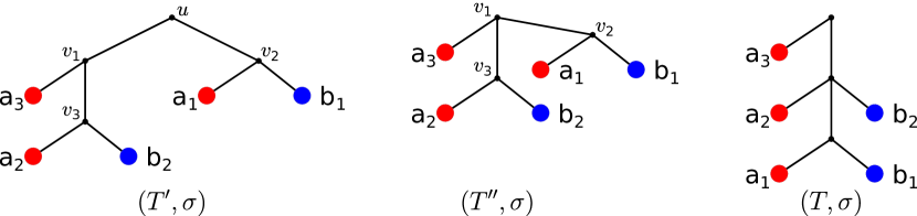
Figure 12: Assume that the tree $(T^{\prime},\sigma)$ is the 2-colored restricted version of some tree that explains a 3-RBMG. It is easy to verify that all three trees $(T^{\prime},\sigma)$, $(T^{\prime\prime},\sigma)$, and $(T,\sigma)$ explain the same 2-RBMG $(G,\sigma)$. According to the transformation of Lemma 17, $(T^{\prime\prime},\sigma)$ is obtained from $(T^{\prime},\sigma)$ by deletion of the edge $uv_{2}$, inserting $v_{1}v_{2}$ and removal of $u$ and its single incident edge. Similarly, $(T,\sigma)$ is obtained from $(T^{\prime\prime},\sigma)$ by deleting $v_{1}v_{2}$ and inserting $v_{3}v_{2}$. The final tree $(T,\sigma)$ is a caterpillar.

Repeated application of the transformation as in Lemma 17 implies the following result, which is illustrated in Fig. 12.

Corollary 5.

Let $(G,\sigma)$ be an $\mathsf{S}$-thin 3-RBMG. Then there exists a tree $(T,\sigma)$ explaining $(G,\sigma)$ for which every 2-colored subtree $(T(u),\sigma_{|L(T(u))})$ with $|\sigma(L(T(u)))|=2$ is a caterpillar and $\sigma(L(T(v_{1})))\neq\sigma(L(T(v_{2})))$ for any distinct $v_{1},v_{2}\in\mathsf{child}(u)$.

Proof.

Let $(T^{\prime},\sigma)$ explain $(G,\sigma)$ and let $u\in V^{0}(T^{\prime})$ be such that $(T^{\prime}(u),\sigma_{|L(T^{\prime}(u))})$ is a 2-colored subtree of $(T^{\prime},\sigma)$. Suppose there exists an inner vertex $v\in V^{0}(T^{\prime}(u))$ with two distinct children that are again inner vertices, i.e., $w_{1},w_{2}\in\mathsf{child}(v)\cap V^{0}(T^{\prime}(u))$. Since $(G,\sigma)$ is $\mathsf{S}$-thin, we can apply Lemma 8 to conclude that $(T^{\prime}(w_{1}),\sigma_{|L(T^{\prime}(w_{1}))})$ and $(T^{\prime}(w_{2}),\sigma_{|L(T^{\prime}(w_{2}))})$ are both 2-colored subtrees, thus $\sigma(L(T^{\prime}(w_{1})))=\sigma(L(T^{\prime}(w_{2})))\subsetneq\sigma(L)$. By Lemma 17, the tree $(T^{\prime\prime},\sigma)$ that is obtained from $(T^{\prime},\sigma)$ by deleting $vw_{2}$ and inserting $w_{1}w_{2}$, still explains $(G,\sigma)$ and satisfies $|\mathsf{child}(v)\cap V^{0}(T^{\prime\prime}(u))|=|\mathsf{child}(v)\cap V^{0}(T^{\prime}(u))|-1$. Repeating this transformation until each inner vertex $v\in V^{0}(T)$ satisfies $\sigma(L(T(v_{1})))\neq\sigma(L(T(v_{2})))$ for any $v_{1},v_{2}\in\mathsf{child}_{T}(v)$, finally yields a tree $(T,\sigma)$ for which $|\mathsf{child}(v)\cap V^{0}(T(u))|\leq 1$, i.e., a caterpillar, that explains $(G,\sigma)$. In particular, we have $|\sigma(L(T(v_{1})))|=1$ if and only if $v_{1}\in L$ (cf. Lemma 8), and $v$ cannot have two leaves of the same color as children because $(G,\sigma)$ is $\mathsf{S}$-thin.

∎

The restriction to connected $\mathsf{S}$-thin graphs with $3$ colors together with the fact that all 2-colored subtrees can be chosen to be caterpillars according to Cor. 5 identifies three distinct classes of trees, see Fig. 6.

Definition 11.

Let $(T,\sigma)$ be a 3-colored tree with color set $S=\{r,s,t\}$. The tree $(T,\sigma)$ is of

Type (I),

if there exists $v\in\mathsf{child}(\rho_{T})$ such that $|\sigma(L(T(v)))|=2$ and $\mathsf{child}(\rho_{T})\setminus\{v\}\subsetneq L$.

Type (II),

if there exists $v_{1},v_{2}\in\mathsf{child}(\rho_{T})$ such that $|\sigma(L(T(v_{1})))|=|\sigma(L(T(v_{2})))|=2$, $\sigma(L(T(v_{1})))\neq\sigma(L(T(v_{2})))$ and $\mathsf{child}(\rho_{T})\setminus\{v_{1},v_{2}\}\subsetneq L$,

Type (III),

if there exists $v_{1},v_{2},v_{3}\in\mathsf{child}(\rho_{T})$ such that $\sigma(L(T(v_{1})))=\{r,s\}$, $\sigma(L(T(v_{2})))=\{r,t\}$, $\sigma(L(T(v_{3})))=\{s,t\}$, and $\mathsf{child}(\rho_{T})\setminus\{v_{1},v_{2},v_{3}\}\subsetneq L$.

Lemma 18.

Let $(G,\sigma)$ be an $\mathsf{S}$-thin connected 3-RBMG with vertex set $L$ and color set $\sigma(L)=\{r,s,t\}$. Then, there is a tree $(T,\sigma)$ with root $\rho_{T}$ explaining $(G,\sigma)$ that satisfies the properties in Cor. 5 and is of Type (I), (II) or (III). In particular, all leaves that are incident to the root of $(T,\sigma)$ must have pairwise distinct colors.

Proof.

Since $(G,\sigma)$ is an RBMG, there is a tree $(T,\sigma)$ that explains $(G,\sigma)$. Denote its root by $\rho_{T}$. Note, $|\sigma(L)|=3$ implies that $|L|\geq 3$.

If $|L|=3$, then it is easy to see that $G$ must be a complete graph on three vertices. In this case, any tree $(T,\sigma)$ where $T$ is a triple explains $(G,\sigma)$ and satisfies Type (I) and Cor. 5.

Now suppose that $|L|>3$. Since $(G,\sigma)$ is connected, Cor. 3(ii) implies that $\zeta(T,\sigma)=\{\rho_{T}\}$. Lemma 14(i) then implies $L\subseteq\mathcal{L}(\rho_{T})\subseteq L$, i.e., $A(\rho_{T})=\mathsf{child}(\rho_{T})$, and thus $|\sigma(L(T(v)))|<3$ for every $v\in\mathsf{child}(\rho_{T})$. This is, every proper subtree of $(T,\sigma)$ contains at most two colors. As a consequence of Cor. 5, the tree $(T,\sigma)$ can be chosen such that there is no pair of distinct vertices $v_{1},v_{2}\in\mathsf{child}(\rho_{T})$ for which $\sigma(L(T(v_{1})))=\sigma(L(T(v_{2})))$. Moreover, as $|L|>3$ and $|\sigma(L)|=3$, it follows directly from Cor. 5 that $|\sigma(L(T(v)))|=1$ for every child $v\in\mathsf{child}(\rho_{T})$ is not possible. Thus, there is at least one child $v\in\mathsf{child}(\rho_{T})$ with $|\sigma(L(T(v)))|\neq 1$ and thus, $|\sigma(L(T(v)))|=2$.

In summary, there are only six possible subtrees $(T(v),\sigma_{L(T(v))})$ with $v\in\mathsf{child}(\rho_{T})$, three containing two colors and three containing only a single color, and each of these six types of subtrees can appear at most once, while there is, in addition, at least one child $v\in\mathsf{child}(\rho_{T})$ where $(T(v),\sigma_{L(T(v))})$ contains two colors.

Therefore, we end up with the three cases (I), (II), and (III): If there is exactly one vertex $v\in\mathsf{child}(\rho_{T})$ such that the subtree $(T(v),\sigma_{L(T(v))})$ contains two colors, any other leaf in $L\setminus L(T(v))$ must be directly attached to $\rho_{T}$, thus Condition (I) is satisfied. Similarly, Condition (II) and (III), respectively, correspond to the case where there exist two and three 2-colored subtrees below the root. Since the three types of trees (I), (II), and (III) differ by the number of two-colored subtrees of the root, no tree can belong to more than one type. By the choice of $(T,\sigma)$, it satisfies Cor. 5.

Finally, if the root of a tree is incident to two leaves of the same color, then the graph explained by this tree cannot be $\mathsf{S}$-thin. Thus, the last statement must be satisfied. ∎

The fact that every connected 3-RBMG can be explained by a tree with a very peculiar structure can now be used to infer stringent structural constraints on the 3-RBMGs themselves.

Lemma 19.

Let $(G,\sigma)$ with vertex set $L$ be an $\mathsf{S}$-thin connected 3-RBMG with $\sigma(L)=\{r,s,t\}$ and $(T,\sigma)$ be a tree of Type (I), (II), or (III) explaining $(G,\sigma)$. Consider $v\in\mathsf{child}(\rho_{T})$ such that $\sigma(L(T(v)))=\{r,s\}$. Then:

• If $x\in L(T(v))\cap L[r]$, then $xy\in E(G)$ for $\sigma(y)=s$ if and only if $\mathsf{par}(x)=\mathsf{par}(y)$ and thus, $y\in L(T(v))$.

If, in addition, there is a vertex $w\in\mathsf{child}(\rho_{T})\setminus\{v\}$ with $\sigma(L(T(w)))=\{r,t\}$, i.e., $(T,\sigma)$ is of either Type (II) or (III), then the following statements hold:

• For any $y\in L(T(v))$, $z\in L(T(w))$, we have $yz\in E(G)$ if and only if $y\in L[s]$ and $z\in L[t]$.

• If $(T,\sigma)$ is of Type (II), then $yz\in E(G)$ for every $y\in L[s]$ and $z\in L[t]$.

• For any $a\in L(T(v))$, $b\in\mathsf{child}(\rho_{T})\cap L$ with $\sigma(b)\neq\sigma(a)$, we have $ab\in E(G)$ if and only if $\sigma(b)\notin\sigma(L(T(v)))$.

Proof.

(i) We assume $y\in L[s]$ and $xy\in E(G)$. For contradiction, suppose $y\notin L(T(v))$. Since $L(T(v))$ contains at least one leaf $y^{\prime}\neq y$ of color $s$, we have $\operatorname{lca}(x,y^{\prime})\preceq v\prec\operatorname{lca}(x,y)$, which implies $xy\notin E(G)$; the desired contradiction. Hence, $y\in L(T(v))$. Now assume, again for contradiction, $\mathsf{par}(x)\neq\mathsf{par}(y)$. There are three cases: (a) $\mathsf{par}(x)$ and $\mathsf{par}(y)$ are incomparable in $(T,\sigma)$, (b) $\mathsf{par}(x)\prec_{T}\mathsf{par}(y)$, or (c) $\mathsf{par}(y)\prec_{T}\mathsf{par}(x)$. In Case (a), Lemma 8 implies that there is a leaf $y^{\prime}\in L(T(\mathsf{par}(x))\cap L[s]$ and therefore, $\operatorname{lca}(x,y^{\prime})\prec\operatorname{lca}(x,y)$; again a contradiction to $xy\in E(G)$. Similar argumentation can be applied to the Cases (b) and (c). Hence, we conclude that $\mathsf{par}(x)=\mathsf{par}(y)$.
Conversely, assume $\mathsf{par}(x)=\mathsf{par}(y)$ and $y\in L(T(v))$. By construction, we have $\mathsf{par}(x)=\operatorname{lca}(x,y)\preceq\operatorname{lca}(x,y^{\prime})$ for all $y^{\prime}\in L[s]$, thus $xy\in E(G)$.

(ii) Let $y\in L(T(v))$, $z\in L(T(w))$ and $yz\in E(G)$. Assume, for contradiction, $\sigma(y)=r$. Since $(G,\sigma)$ does not contain edges between vertices of the same color, we have $z\in L[t]$. By construction of $(T,\sigma)$, there must be some $x\in L(T(w))$ of color $r$. Hence, $\operatorname{lca}(z,x)\preceq w\prec\operatorname{lca}(z,y)=\rho_{T}$; a contradiction to $yz\in E(G)$. Thus, $\sigma(y)=s$. An analogous argument yields $\sigma(z)=t$. Conversely, let $y\in L(T(v))$ and $z\in L(T(w))$ such that $\sigma(y)=s$ and $\sigma(z)=t$. Since neither $t\in\sigma(L(T(v)))$ nor $s\in\sigma(L(T(w)))$ and $(T,\sigma)$ is of Type (II) or (III), we can immediately conclude that $\operatorname{lca}(y,z)=\rho_{T}=\operatorname{lca}(y,z^{\prime})=\operatorname{lca}(y^{\prime},z)$ for all $y^{\prime}\in L[s]$ and all $z^{\prime}\in L[t]$. Thus, $yz\in E(G)$.

(iii) Since, $s\notin\sigma(L(T(w)))$, $t\notin\sigma(L(T(v)))$, and $(T,\sigma)$ is of Type (II), we have $\operatorname{lca}_{T}(y,z)=\rho_{T}$ for any pair $y\in L[s]$, $z\in L[t]$. Thus, $yz\in E(G)$.

(iv) Let $\sigma(a)=r$ and suppose first $\sigma(b)=s$. Then, there is some $y\prec v$ with $\sigma(y)=s$, thus $\operatorname{lca}(a,y)\prec\operatorname{lca}(a,b)$. Therefore $a$ and $b$ cannot be reciprocal best matches, i.e., $ab\notin E(G)$. Now assume $\sigma(b)=t$. Since $t\notin\sigma(L(T(v)))$, we have $\operatorname{lca}(a,z)=\rho_{T}$ for every $z\in L[t]$. In particular, we have $\operatorname{lca}(b,L[r])=\rho_{T}$, and therefore $ab\in E(G)$.

∎

We note in passing that Lemma 19(iv) is also satisfied by Type (I) trees.

In the following we also need a special form of Type (II) trees:

Definition 12.

A tree $(T,\sigma)$ of Type (II) with color set $S=\{r,s_{1},s_{2}\}$ and root $\rho_{T}$, where $v_{1},v_{2}\in\mathsf{child}(\rho_{T})$ with $\sigma(L(T(v_{1})))=\{r,s_{1}\}$ and $\sigma(L(T(v_{2})))=\{r,s_{2}\}$, is of Type (II^∗) if, for $i\in\{1,2\}$, it satisfies:

($\star$)

If there is a vertex $w\in V^{0}(T(v_{i}))$ such that $\mathsf{child}(w)\cap L=\{x\}$ for some $x\in L[r]$, then there is a vertex $v\in\mathsf{child}(\rho_{T})$ such that $\sigma(v)=s_{i}$.

For leaf-colored trees explaining an $\mathsf{S}$-thin graph, Definition 12 implies, in particular, that if there is some vertex $w\in V^{0}(T(v_{i}))$ with $\sigma(\mathsf{child}(w)\cap L)=\{r\}$ in a tree $(T,\sigma)$ of Type (II^∗), then $L[s_{i}]\setminus L(T(v_{i}))\neq\emptyset$. Moreover, note that in a leaf-colored tree explaining an $\mathsf{S}$-thin graph, the property $\sigma(\mathsf{child}(w)\cap L)=\{r\}$ always implies $|\mathsf{child}(w)\cap L|=1$.

Given an arbitrary tree $(T,\sigma)$ of Type (II) with colors and subtrees as in Def. 12, one can easily construct a corresponding tree $(T^{\prime},\sigma)$ of Type (II^∗) using the following rule for $i\in\{1,2\}$:

(r)

If there is no vertex $v\in\mathsf{child}(\rho_{T})$ such that $\sigma(v)=s_{i}$, then re-attach all vertices $x\in L[r]$ with $\mathsf{child}(\mathsf{par}(x))\cap L=\{x\}$ to $\rho_{T}$ and suppress $\mathsf{par}(x)$ in case $\mathsf{par}(x)$ has degree 2 after removal of the edge $\mathsf{par}(x)x$.

By construction, the tree $(T^{\prime},\sigma)$ has no vertices $w\in V^{0}(T(v_{i}))$ with $\sigma(\mathsf{child}(w)\cap L)=\{r\}$, and thus, $(T^{\prime},\sigma)$ trivially satisfies ($\star$). Hence, $(T^{\prime},\sigma)$ is of Type (II^∗).

We proceed by showing that rule (r) must be applied to at most one leaf in order to obtain a tree $(T^{\prime},\sigma)$ of Type (II^∗).

Lemma 20.

Let $(T,\sigma)$ be Type (II) tree that is not of Type (II^∗) and that explains a connected $\mathsf{S}$-thin 3-RBMG. Let $\rho_{T}$ be the root of $(T,\sigma)$ and $S=\{r,s_{1},s_{2}\}$ its color set. Moreover, let $v_{1},v_{2}\in\mathsf{child}(\rho_{T})$ such that $\sigma(L(T(v_{i})))=\{r,s_{i}\}$, $i\in\{1,2\}$. Then,

1. no leaf of color $r$ is incident to $\rho_{T}$ and

2. if Rule (r) is applied to some vertex $x\in L(T(v_{i}))$, then $x$ is the only leaf in $L[r]\cap L(T(v_{i}))$ with $\mathsf{child}(\mathsf{par}(x))\cap L=\{x\}$ and all inner vertices in $L(T(v_{j}))$, $j\neq i$ satisfy Property ($\star$) in Def. 12.

Proof.

First note that, since $(T,\sigma)$ is of Type (II), it satisfies $\mathsf{child}(\rho_{T})\setminus\{v_{1},v_{2}\}\subset L$. Since $(T,\sigma)$ is not of Type (II^∗), there must be a leaf $x\in L[r]$ with $w\coloneqq\mathsf{par}(x)\preceq_{T}v_{i}$ and $\sigma(\mathsf{child}(w)\cap L)=\{r\}$ such that there is no leaf of color $s_{i}$ incident to $\rho_{T}$, i.e., $L[s_{i}]\subseteq L(T(v_{i}))$ for some $i\in\{1,2\}$. W.l.o.g. we can assume $i=1$. Now, $L[s_{1}]\subseteq L(T(v_{1}))$ and Lemma 19(i) implies that $N_{s_{1}}(x)=\emptyset$ in $(G,\sigma)$. However, since $(G,\sigma)$ is connected, there must exist some $z\in L[s_{2}]$ such that $xz\in E(G)$. Lemma 19(i)+(iv) then implies that every $z\in L[s_{2}]$ with $xz\in E(G)$ must be incident to $\rho_{T}$. However, Lemma 18 implies that $z$ is the only leaf of color $s_{2}$ that is incident to the root. Since $N_{s_{1}}(x)=\emptyset$, it holds that $z$ is the only vertex in $L$ that is adjacent to $x$ in $G$ and thus, $N(x)=\{z\}$ in $(G,\sigma)$.

In order to show Statement (i), we now assume for contradiction that there exists another leaf $x^{\prime}\neq x$ of color $r$ such that $x^{\prime}\in\mathsf{child}(\rho_{T})$. Then, as a consequence of Lemma 18 and since $L[s_{1}]\subseteq L(T(v_{1}))$, we have $\mathsf{child}(\rho_{T})\cap L=\{x^{\prime},z\}$. Thus Lemma 19(i)+(iv) implies that $x^{\prime}$ is not adjacent to any vertex in $L(T(v_{1}))\cup L(T(v_{2}))$. Moreover, we have $\operatorname{lca}_{T}(x^{\prime},z)=\rho_{T}=\operatorname{lca}_{T}(x^{\prime\prime},z)=\operatorname{lca}_{T}(x^{\prime},z^{\prime})$ for all $x^{\prime\prime}\in L[r]$ and $z^{\prime}\in L[s_{2}]$, hence $x^{\prime}z\in E(G)$. Taking the latter two arguments together with the observation that there is no leaf with color $s_{1}$ incident to the root $\rho_{T}$, we obtain $N(x^{\prime})=N(x)=\{z\}$ in $(G,\sigma)$; a contradiction to the $\mathsf{S}$-thinness of $(G,\sigma)$.

We proceed with showing Statement (ii). Repeating the latter arguments, one easily checks that $N(x_{1})=\{z\}$ for any vertex $x_{1}\in L(T(v_{1}))$ with $\sigma(\mathsf{child}(\mathsf{par}(x_{1}))\cap L)=\{r\}$. However, since $(G,\sigma)$ is $\mathsf{S}$-thin, we cannot have a further vertex $x_{1}\in L(T(v_{1}))$ with $N(x_{1})=\{z\}=N(x)$. Hence, there is exactly one $x\in L[r]\cap L(T(v_{1}))$ with $\mathsf{child}(\mathsf{par}(x))\cap L=\{x\}$ to which Rule (r) can be applied. Moreover, the existence of $z\in\mathsf{child}(\rho_{T})\cap L[s_{2}]$ immediately implies that Property ($\star$) in Def. 12 is satisfied for every $w\in V^{0}(T(v_{2}))$ with $\sigma(\mathsf{child}(w)\cap L)=\{r\}$. Thus, Statement (ii) is satisfied. ∎

Lemma 21.

If a connected $\mathsf{S}$-thin 3-RBMG can be explained by tree of Type (II), then it can be explained by a tree of Type (II^∗).

Proof.

Assume that $(T,\sigma)$ is of Type (II) and that $G(T,\sigma)$ is a connected $\mathsf{S}$-thin 3-RBMG. Let $S=\{r,s,t\}$ be the color set of $L\coloneqq L(T)$ and $v_{1},v_{2}\in\mathsf{child}(\rho_{T})$ with $\sigma(L(T(v_{1})))=\{r,s\}$ and $\sigma(L(T(v_{2})))=\{r,t\}$. If $(T,\sigma)$ is already of Type (II^∗), then the statement is trivially true.

Now suppose that $(T,\sigma)$ is not of Type (II^∗). Lemma 20 implies that there is exactly one leaf $x\in L[r]$ to which Rule (r) can be applied. Hence, by using Rule (r) and thus re-attaching $x$ to the root, one obtains a tree $(T^{\prime},\sigma)$ of Type (II^∗). In particular, Lemma 20 implies that $x$ is the only vertex with color $r$ in $(T^{\prime},\sigma)$ incident to the root. W.l.o.g. assume that $x\in L(T(v_{1}))$. Note, in particular, that the necessity of relocating $x$ implies $L[s]\setminus L(T(v_{1}))=\emptyset$ (cf. Rule (r)), i.e., $L[s]\subseteq L(T(v_{1}))$. Thus, $\mathsf{child}(\mathsf{par}(x))\cap L=\{x\}$ and Lemma 19(i)+(iv) implies that $N_{s}(x)=\emptyset$ in $G(T,\sigma)$.

Since $L=L(T^{\prime})$, it suffices to show that $E(G(T^{\prime},\sigma))=E(G(T,\sigma))$ to prove that $(T^{\prime},\sigma)$ explains $G(T,\sigma)$. One easily checks that the only edges that may be different between both sets are those containing the leaf $x$.

We start by showing $N_{s}(x)=\emptyset$ in $G(T^{\prime},\sigma)$. Observe first that, as we have only changed the position of vertex $x\in L[r]$ to obtain $(T^{\prime},\sigma)$, $L[s]\subseteq L(T(v_{1}))$ implies $L[s]\subseteq L(T^{\prime}(v_{1}))$. By Lemma 8, we have $\sigma(L(T(w)))=\{r,s\}$ for all inner vertices $w\preceq_{T}v_{1}$ in $T$. Thus, there must be a vertex $w\in(L(T(v_{1})))$ that is incident to two leaves $x^{\prime}$ and $y$ with $\sigma(x^{\prime})=r$ and $\sigma(y)=s$. Since $\{x^{\prime},y\}\subseteq\mathsf{child}(\mathsf{par}(y))$, it follows $x^{\prime}\neq x$ and thus, $x^{\prime}$ has not been re-attached. The latter implies that $\sigma(L(T^{\prime}(v_{1})))=\{r,s\}$ and, by construction, $\operatorname{lca}_{T^{\prime}}(x,y^{\prime})=\rho_{T^{\prime}}\succ_{T^{\prime}}v_{1}\succ_{T^{\prime}}\operatorname{lca}_{T^{\prime}}(x^{\prime},y^{\prime})$ for all $x^{\prime}\in L(T^{\prime}(v_{1}))\cap L[r]$ and $y^{\prime}\in L[s]\cap L(T^{\prime}(v_{1}))=L[s]$. Therefore, there is no edge between $x$ and any $y^{\prime}\in L[s]$ in $G(T^{\prime},\sigma)$. Hence, $N_{s}(x)=\emptyset$ in $G(T^{\prime},\sigma)$.

It remains to show that $xz\in E(G(T,\sigma))$ if and only if $xz\in E(G(T^{\prime},\sigma))$ for this particular re-located vertex $x$ and all $z\in L[t]$. Since $G(T,\sigma)$ is connected and $N_{s}(x)=\emptyset$, there must exist some vertex $z$ with color $t$ such that $xz\in E(G(T,\sigma))$. Note, Lemma 19(ii) implies that there are no edges $xz$ for all $z\in L[t]\cap L(T(v_{2}))$. That is, $x$ and $z\in L[t]$ form an edge $xz$ in $G(T,\sigma)$ if and only if $z$ is incident to the root $\rho_{T}$ (cf. Lemma 19(ii)+(iv)). In particular, we have by construction of $(T^{\prime},\sigma)$ that $\operatorname{lca}_{T^{\prime}}(x,z)=\rho_{T^{\prime}}=\operatorname{lca}_{T^{\prime}}(x^{\prime},z)=\operatorname{lca}_{T^{\prime}}(x,z^{\prime})$ for all $x^{\prime}\in L[r]$ and all $z^{\prime}\in L[t]$ and hence, $xz\in E(G(T^{\prime},\sigma))$.

Now assume that $xz\in E(G(T^{\prime},\sigma))$ for this particular re-located vertex $x$ and some $z\in L[t]$. Since $x$ has been re-attached, we have $\operatorname{lca}_{T^{\prime}}(x,z)=\rho_{T^{\prime}}$. By Lemma 20, none of the vertices in $L(T(v_{2}))$ has been re-attached. Hence, $L(T^{\prime}(v_{2}))=L(T(v_{2}))$ and thus, $\sigma(L(T(v_{2})))=\{r,t\}$. Moreover, we have $xz^{\prime}\notin E(G(T^{\prime},\sigma))$ for all $z^{\prime}\in L[t]\cap L(T(v_{2}))$ since $\operatorname{lca}_{T^{\prime}}(x,z^{\prime})=\rho_{T^{\prime}}\succ_{T^{\prime}}\operatorname{lca}_{T^{\prime}}(x^{\prime},z^{\prime})$ for all $x^{\prime}\in L[r]\cap L(T(v_{2}))$. Thus, $z$ must be adjacent to $\rho_{T^{\prime}}$. By construction, $z$ must be adjacent to $\rho_{T}$. As argued above, $xz$ in $G(T,\sigma)$ if and only if $z$ is incident to the root $\rho_{T}$. Therefore, $xz\in E(G(T,\sigma))$.

In summary, $E(G(T^{\prime},\sigma))=E(G(T,\sigma))$ and hence, $(T^{\prime},\sigma)$ explains $G(T,\sigma)$. ∎

D.2 Three classes of $\mathsf{S}$-thin $3$-RBMGs

We are now in the position to use these results to show that connected components of 3-RBMGs can be grouped into three disjoint graph classes that correspond to the three tree Types (I), (II), and (III). These three classes are shown in Fig. 6.

Definition 13.

An undirected, connected graph $(G,\sigma)$ on three colors is of

Type (A)

if $(G,\sigma)$ contains a $K_{3}$ on three colors but no induced $P_{4}$, and thus also no induced $C_{n}$, $n\geq 5$.

Type (B)

if $(G,\sigma)$ contains an induced $P_{4}$ on three colors whose endpoints have the same color, but no induced $C_{n}$ for $n\geq 5$.

Type (C)

if $(G,\sigma)$ contains an induced $C_{6}$ along which the three colors appear twice in the same permutation, i.e., $(r,s,t,r,s,t)$.

Theorem 4.

Let $(G,\sigma)$ be an $\mathsf{S}$-thin connected 3-RBMG. Then $(G,\sigma)$ is either of Type (A), (B), or (C). An RBMG of Type (A), (B), and (C), resp., can be explained by a tree of Type (I), (II), and (III), respectively.

Proof.

Let $(G,\sigma)$ be an $\mathsf{S}$-thin connected 3-RBMG. If $|L|=3$, then $|\sigma(L)|=3$ implies that $(G,\sigma)$ is the complete graph $K_{3}$ on three colors, i.e., a graph of Type (A). Every phylogenetic tree on three leaves explains $(G,\sigma)$, and all of them except the star are of Type (I). From here on we assume $|L|>3$. By Lemma 18 every connected $\mathsf{S}$-thin 3-RBMG $(G,\sigma)$ is explained by a tree $(T,\sigma)$ of either Type (I), (II), or (III).

Claim 1. If $(T,\sigma)$ is of Type (I), then $(G,\sigma)$is of Type (A).

Proof of Claim 1. Let $(T,\sigma)$ be a Type (I) tree, i.e., the root $\rho_{T}$ has one child $v$ such that $\sigma(L(T(v)))=\{r,s\}$ and all other children of $\rho_{T}$ are leaves. This and $|\sigma(L)|=3$ implies that there must be a leaf $z\in\mathsf{child}(\rho_{T})\cap L[t]$. Since $(G,\sigma)$ is $\mathsf{S}$-thin, $z$ is the only leaf of color $t$ in $(T,\sigma)$, thus $xz\in E(G)$ for every $x\in L[r]$ and $yz\in E(G)$ for every $y\in L[s]$. In particular, Lemma 8 implies that there exists an inner vertex $u\preceq_{T}v$ such that $\mathsf{child}(u)=\{x^{*},y^{*}\}$ with $x^{*}\in L[r]$ and $y^{*}\in L[s]$, thus we have $x^{*}y^{*}\in E(G)$. Hence, the induced subgraph $G[x^{*}y^{*}z]$ forms a $K_{3}$.

It remains to show that $(G,\sigma)$ contains no induced $C_{n}$, $n\geq 5$, or $P_{4}$. Since $L[t]=\{z\}$ and $xz,yz\in E(G)$ for any $x\in L[r]$ and $y\in L[s]$, we can conclude that there cannot be any induced $P_{4}$, and thus no induced $C_{n}$, $n\geq 5$, either, that contains color $t$. Now assume, for contradiction, that there is an induced $P_{4}$ that contains the two colors $r,s$. By construction, this $P_{4}$ must have subsequent coloring $(r,s,r,s)$, thus it contains three distinct vertices $x,y_{1},y_{2}$ such that $x\in L[r]$ and $y_{1},y_{2}\in L[s]$ and $x$ is adjacent to $y_{1}$ and $y_{2}$. Lemma 19(i) implies that $\mathsf{par}(y_{1})=\mathsf{par}(y_{2})$. Hence, $N(y_{1})=N(y_{2})$, which contradicts the $\mathsf{S}$-thinness of $(G,\sigma)$. Thus, there exists no induced $P_{4}$ and thus no induced $C_{n}$ with $n\geq 5$ containing only two colors.

Hence, $(G,\sigma)$ is of Type (A). $\triangleleft$

Claim 2. If $(T,\sigma)$ is of Type (II), then $(G,\sigma)$ is of Type (B).

Proof of Claim 2. Let $(T,\sigma)$ be a Type (II) tree, i.e., the root has two distinct children $v_{1},v_{2}\in\mathsf{child}(\rho_{T})$ such that $\sigma(L(T(v_{1})))=\{r,s\}$ and $\sigma(L(T(v_{2})))=\{r,t\}$, and all other children of the root are leaves.

We start by showing that $(G,\sigma)$ contains the particular colored induced $P_{4}$. Lemma 8 implies that there must be a leaf $y_{1}\in L(T(v_{1}))\cap L[s]$ such that $\mathsf{par}(y_{1})=\mathsf{par}(x_{1})$ for some $x_{1}\in L(T(v_{1}))\cap L[r]$ and therefore $x_{1}y_{1}\in E(G)$. Similarly, there exist two leaves $z_{1}\in L(T(v_{2}))\cap L[t]$ and $x_{2}\in L(T(v_{2}))\cap L[r]$ such that $x_{2}z_{1}\in E(G)$. Lemma 19(ii) implies that $x_{1}z_{1}\notin E(G)$ and $x_{2}y_{1}\notin E(G)$. Clearly, $x_{1}x_{2}\notin E(G)$ since the two vertices have the same color. Moreover, Lemma 19(iii) implies that $y_{1}z_{1}\in E(G)$. Hence, $\langle x_{1}y_{1}z_{1}x_{2}\rangle$ forms an induced $P_{4}$ in $(G,\sigma)$ on three colors whose endpoints have the same color.

We proceed by showing that $(G,\sigma)$ does not contain an induced $C_{n}$ with $n\geq 5$. First note that Lemma 19(iii) implies $yz\in E(G)$ for any two leaves $y\in L[s]$, $z\in L[t]$. Thus, $(G,\sigma)$ cannot contain an induced $C_{n}$ for some $n\geq 5$ on colors $s$ and $t$ only. Therefore, assume, for contradiction, that there exists an induced $C_{n}$ for some fixed $n\geq 5$ in $G(T,\sigma)$ that contains a leaf $x$ of color $r$. Note that this necessarily implies $|N(x)|>1$ in $G$. Suppose first that $x\in\mathsf{child}(\rho_{T})$. Since $(T(v_{1}),\sigma_{|L(T(v_{1}))})$ and $(T(v_{2}),\sigma_{|L(T(v_{2}))})$ both contain leaves of color $r$, any vertex that is adjacent to $x$ in $G$ must be incident to $\rho_{T}$ in $T$. Hence, as $(G,\sigma)$ is $\mathsf{S}$-thin, $|N(x)|>1$ in $G$ implies that $\mathsf{child}(\rho_{T})\cap L=\{x,y,z\}$, where $y\in L[s]$ and $z\in L[t]$, i.e., we have $N(x)=\{y,z\}$. Thus, any induced $C_{n}$, $n\geq 5$ containing $x$ must also contain both $y$ and $z$. However, as $x$, $y$, and $z$ have the same parent in $T$, they clearly form a $K_{3}$ in $G$; a contradiction to $x$, $y$, and $z$ being part of an induced $C_{n}$.

Now suppose $x\in L(T(v_{1}))\cap L[r]$. Since $(T(v_{2}),\sigma_{|L(T(v_{2}))})$ contains the colors $r$ and $t$, $(G,\sigma)$ cannot contain an edge $xz$ with $z\in L(T(v_{2}))$ (cf. Lemma 19(ii)). Hence, $N_{t}(x)\neq\emptyset$ if and only if there exists a leaf $z$ of color $t$ that is directly attached to the root $\rho_{T}$. Since $G(T,\sigma)$ is $\mathsf{S}$-thin, there can be at most one leaf of color $t$ that is attached to $\rho_{T}$, thus $|N_{t}(x)|\leq 1$. This and $|N(x)|>1$ in $G$ implies that there must be a leaf $y\in L[s]$ such that $y\in N_{s}(x)$. By Lemma 19(i), this is the case if and only if $y\in L(T(v_{1}))\cap L[s]$ and $\mathsf{par}(x)=\mathsf{par}(y)$. Since $G(T,\sigma)$ is $\mathsf{S}$-thin, there exists at most one leaf of color $s$ with this property, hence in particular $N(x)=\{y,z\}$. Using Lemma 19(iv), we can conclude that $yz\in E(G)$. Thus, $x$, $y$ and $z$ form a $K_{3}$. Therefore, these three leaves cannot be contained together in an induced $C_{n}$, $n\geq 5$.

Since an analogous argumentation holds if $x\in L(T(v_{2}))$, we conclude that there cannot be an induced $C_{n}$, $n\geq 5$ containing a leaf of color $r$.

In summary, $G$ does not contain an induced $C_{n}$ for $n\geq 5$, and thus, $(G,\sigma)$ is of Type (B). $\triangleleft$

Claim 3. If $(T,\sigma)$ is of Type (III), then $(G,\sigma)$ is of Type (C).

Proof of Claim 3. Let $(T,\sigma)$ be a Type (III) tree, i.e., the root $\rho_{T}$ has three children $v_{1},v_{2},v_{3}\in\mathsf{child}(\rho_{T})$ such that $\sigma(L(T(v_{1})))=\{r,s\}$, $\sigma(L(T(v_{2})))=\{r,t\}$, and $\sigma(L(T(v_{3})))=\{s,t\}$, and all remaining children are leaves. Again, Lemma 8 and Lemma 19(i) imply that there exist $x_{1},y_{1}\in L(T(v_{1}))$ with $x_{1}y_{1}\in E(G)$, $x_{2},z_{1}\in L(T(v_{2}))$ with $x_{2}z_{1}\in E(G)$ and $y_{2},z_{2}\in L(T(v_{3}))$ with $y_{2}z_{2}\in E(G)$, where $x_{i}\in L[r]$, $y_{i}\in L[s]$ and $z_{i}\in L[t]$. Applying Lemma 19(ii), we can in addition conclude that $y_{1}z_{1},x_{2}y_{2},x_{1}z_{2}\in E(G)$, and $(G,\sigma)$ contains none of the edges $x_{1}z_{1}$, $x_{1}y_{2}$, $y_{1}x_{2}$, $y_{1}z_{2}$, $z_{1}y_{2}$, or $x_{2}z_{2}$. Moreover, $(G,\sigma)$ does not contain edges between vertices of the same color. Hence, $(G[C],\sigma_{|C})$ with $C=\{x_{1},y_{1},z_{1},x_{2},y_{2},z_{2}\}$ forms the desired induced $C_{6}$. Therefore, $(G,\sigma)$ is of Type (C). $\triangleleft$

By definition, the three classes of 3-RBMGs (A), (B), and (C) are disjoint. Lemma 18 states that the three classes of trees (I), (II), and (III) are disjoint, hence there is a 1-1 correspondence between the tree Types (I), (II), and (III) and the graph classes (A), (B), and (C).

∎

An undirected, colored graph $(G,\sigma)$ contains an induced $K_{3}$, $P_{4}$, or $C_{6}$, respectively, if and only if $(G/\mathsf{S},\sigma/\mathsf{S})$ contains an induced $K_{3}$, $P_{4}$, or $C_{6}$, resp., on the same colors (cf. Lemma 5). An immediate consequence of this fact is

Theorem 5.

A connected (not necessarily $\mathsf{S}$-thin) 3-RBMG $(G,\sigma)$ is either of Type (A), (B), or (C).

D.3 Characterization of Type (A) 3-RBMGs

As an immediate consequence of Theorem 4 and the well-known properties of cographs [Corneil et al., 1981] we obtain

Observation 3.

Let $(G,\sigma)$ be a connected, $\mathsf{S}$-thin 3-RBMG. Then it is of Type (A) if and only if it is a cograph.

Definition 14.

Let $G=(V,E)$ be an undirected graph. A vertex $x\in V(G)$ such that $N(x)=V\setminus\{x\}$ is a hub-vertex.

Lemma 22.

A properly vertex colored, connected, $\mathsf{S}$-thin graph $(G,\sigma)$ on three colors with vertex set $L$ is a 3-RBMG of Type (A) if and only if $G\notin\mathscr{P}_{3}$ and it satisfies the following conditions:

1. $G$ contains a hub-vertex $x$, i.e., $N(x)=V(G)\setminus\{x\}$

2. $|N(y)|<3$ for every $y\in V(G)\setminus\{x\}$.

Proof.

By definition, a 3-RBMG is properly colored and has $|L|\geq 3$ vertices. If $|L|=3$ there are only two connected graphs: $K_{3}$ and $P_{3}$. Both satisfy (A1) and (A2) since the three vertices have distinct colors. However, only $K_{3}$ is a 3-RBMG: it is explained by any tree on three leaves with pairwise distinct colors. From here on we assume $|L|\geq 4$.

We start with the “only-if-direction” and show that every 3-RBMG of Type (A) satisfies (A1) and (A2). We set $S=\{r,s,t\}$, and assume that $(G,\sigma)$ is a 3-RBMG of Type (A). Theorem 4 implies that there exists a tree $(T,\sigma)$ with root $\rho_{T}$ explaining $(G,\sigma)$ that is of Type (I), i.e., there is a vertex $v\in\mathsf{child}(\rho_{T})$ such that $\sigma(L(T(v)))=\{s,t\}$ and $\mathsf{child}(\rho_{T})\setminus\{v\}\subset L$. Thus every leaf $x$ with color $\sigma(x)=r$ is a child of $\rho_{T}$. Since $(G,\sigma)$ is $\mathsf{S}$-thin, this implies $|L[r]|=1$ and therefore, $xy\in E(G)$ for every $y\neq x$, hence (A1) is satisfied. In order to show (A2), consider $y\in V(G)\setminus\{x\}$, where $x$ is again the unique vertex with color $r$. Since $(G,\sigma)$ is properly colored, $\sigma(y)\neq r$. W.l.o.g., let $\sigma(y)=s$. Assume, for contradiction, that $|N(y)|\geq 3$. Then there are at least two distinct vertices $z,z^{\prime}\in N_{t}(y)$. Assume first that $y\in L(T(v))$. Hence, there is $z^{*}\in L[t]$ with $\operatorname{lca}(y,z^{*})\preceq v\prec\rho_{T}$. Hence, we must have $z,z^{\prime}\in L(T(v))$. However, Lemma 19(i) implies that $z$ and $z^{\prime}$ must be siblings and therefore $N(z)=N(z^{\prime})$; a contradiction, since $(G,\sigma)$ was assumed to be $\mathsf{S}$-thin. Now assume that $y\in\mathsf{child}(\rho_{T})$. Then, Lemma 19(iv) and $z,z^{\prime}\in N_{t}(y)$ imply that $z$ and $z^{\prime}$ both have to be adjacent to $\rho_{T}$; again this contradicts the assumption that $(G,\sigma)$ is $\mathsf{S}$-thin. Thus, (A2) is satisfied.

We proceed with showing the “if-direction”. Suppose $(G,\sigma)$ is a properly vertex colored, connected, $\mathsf{S}$-thin graph satisfying (A1) and (A2). In order to show that $(G,\sigma)$ is a Type (A) RBMG it suffices, by Theorem 4, to construct a Type (I) tree that explains $(G,\sigma)$. Let $x$ be a vertex that is adjacent to all others, which exists by (A1). Assume w.l.o.g. that $\sigma(x)=r$. Since $(G,\sigma)$ is $\mathsf{S}$-thin and it does not contain edges between vertices of the same color, $x$ must be the only vertex of color $r$. We define $L_{2}\coloneqq\{y\mid y\neq x,|N(y)|=2\}$. Since $|L|>3$ and thus $|N(x)|\geq 3$, we have $x\in L\setminus L_{2}$. Note, each vertex is adjacent to $x$ and thus, $N(y)=\{x,z\}$ for all $y\in L_{2}$ and some vertex $z\in L[t]$, $t\neq\sigma(y)$. Property (A2) implies that there are $|L\setminus L_{2}|-1$ vertices with degree $1$, all incident to $x$. Since $(G,\sigma)$ is $\mathsf{S}$-thin and $|S|=3$, there are at most two vertices with degree $1$, at most one of each color different from $\sigma(x)$, and thus $|L\setminus L_{2}|\leq 3$.

We first construct a caterpillar $(T_{2},\sigma_{|L_{2}})$ with leaf set $L_{2}$ and root $\rho_{T_{2}}$ such that $\mathsf{par}(y)=\mathsf{par}(z)$ for any $y,z\in L_{2}$ with $\sigma(y)\neq\sigma(z)$ if only if $yz\in E(G)$. As $N(y)=\{x,z\}$ for all $y\in L_{2}$ and some vertex $z\in L[t]$, $t\neq\sigma(y)$, we can conclude that each connected component of $(G[L_{2}],\sigma_{|L_{2}})$ is a single edge $yz$. Thus, it is easy to see that $(T_{2},\sigma_{|L_{2}})$ explains $(G[L_{2}],\sigma_{|L_{2}})$.

For the construction of $(T,\sigma)$, we then distinguish two cases: (i) If $L\setminus L_{2}=\{x,w_{1}\}$, then $(T,\sigma)$ is obtained by attaching the vertices $x$ and $w_{1}$ as well as $\rho_{T_{2}}$ as children of the root $\rho_{T}$. (ii) If $L\setminus L_{2}=\{x,w_{1},w_{2}\}$ for distinct vertices $x$, $w_{1}$, and $w_{2}$ in $(G,\sigma)$, we first build an auxiliary tree $(T^{\prime},\sigma_{|L_{2}\cup\{w_{2}\}})$ with root $\rho_{T^{\prime}}$ by attaching $\rho_{T_{2}}$ and vertex $w_{2}$ to $\rho_{T^{\prime}}$. The tree $(T,\sigma)$ is then constructed from $(T^{\prime},\sigma_{|L_{2}\cup\{w_{2}\}})$ by attaching $x$, the other vertex $w_{1}$ and $\rho_{T^{\prime}}$ as children of $\rho_{T}$. It remains to show that $(T,\sigma)$ explains $(G,\sigma)$. By construction, $(T,\sigma)$ is a tree of Type (I) where the vertices $\rho_{T_{2}}$ and $\rho_{T^{\prime}}$ play the role of $v$ in Def. 12 in Case (i) and (ii), respectively. In the following let $v=\rho_{T_{2}}$ or $v=\rho_{T^{\prime}}$ depending on whether we have Case (i) and (ii).

Theorem 4 implies that $G(T,\sigma)$ is 3-RBMG of Type (A). It is easy to see that $G(T,\sigma)[L_{2}]=(G[L_{2}],\sigma_{|L_{2}})$. Any remaining edges in $G(T,\sigma)$ are thus adjacent to vertices in $L\setminus L_{2}$. We first consider edges that may be incident to vertex $x$ in $G(T,\sigma)$. Since $\operatorname{lca}_{T}(z,x)=\rho_{T}$ and $r\notin\sigma(L(T(v)))$, we have $xz\in E(G(T,\sigma))$ for all $z\in L\setminus\{x\}$. Hence, (A1) is satisfied by $x$ in $G(T,\sigma)$.

Now, consider edges that may be incident to vertex $w_{1}$ in $G(T,\sigma)$. First note, that in both Cases (i) and (ii), the vertex $w_{1}$ is adjacent to the root $\rho_{T}$ in $(T,\sigma)$. Since $(T,\sigma)$ is a tree of Type (I), we can apply Lemma 19(i) to conclude that there are no edges in $G(T,\sigma)$ between $w_{1}$ and any vertex in $L(T(v))$. This and the arguments above show that $N(w_{1})=\{x\}$. In other words, $w_{1}z\in E(G(T,\sigma))$ if and only if $w_{1}z\in E(G)$ for all $z\in L$. This in particular shows $(G,\sigma)=G(T,\sigma)$ conforms to Case (i).

Finally, assume Case (ii) and consider edges that are incident to vertex $w_{2}$ in $(G,\sigma)$ By construction, $s,t\in\sigma(L_{2})$. Since $\operatorname{lca}(w_{2},z)=v\succ_{T}\rho_{T_{2}}\succeq\operatorname{lca}(w^{\prime},z)$ for all $w^{\prime},z\in L_{2}$ with $\sigma(w_{2})=\sigma(w)\neq\sigma(z)$, we can conclude that $w_{2}$ is not adjacent to any other vertex in $L_{2}$. This and the arguments above show that $N(w_{2})=\{x\}$. Therefore, $w_{2}z\in E(G(T,\sigma))$ if and only if $w_{1}z\in E(G)$ for all $z\in L$.

In summary, $G(T,\sigma)=(G,\sigma)$. Therefore, $(G,\sigma)$ is of Type (A).

∎

For later reference, we record a simple property of hub-vertices.

Corollary 6.

Let $x$ be a hub-vertex of some connected $\mathsf{S}$-thin 3-RBMG $(G,\sigma)$ of Type (A) with vertex set $L$ and $|L|>3$. Then, $x$ is the only vertex of its color in $(G,\sigma)$, i.e., $L[\sigma(x)]=\{x\}$. Moreover, for any $(T,\sigma)$ explaining $(G,\sigma)$, $x$ must be incident to the root of $T$.

Proof.

Since $(G,\sigma)$ does not contain edges between vertices of the same color, the first statement immediately follows from Property (A1) and $\mathsf{S}$-thinness of $(G,\sigma)$.

For the second statement, let $(T,\sigma)$ be an arbitrary tree with root $\rho_{T}$ that explains $(G,\sigma)$. Let $v\in\mathsf{child}(\rho_{T})$ with $x\preceq_{T}v$. Assume, for contradiction, $v\neq x$. Thus Lemma 8 implies that there exists a leaf $y\in L$ with $\sigma(y)\neq\sigma(x)$ such that $y\preceq_{T}v$. Then, since $x$ is connected to any vertex in $L\setminus\{x\}$, all vertices of color $\sigma(y)$ must be contained in the subtree $T(v)$; otherwise $\operatorname{lca}_{T}(x,y)\prec_{T}\operatorname{lca}_{T}(x,y^{\prime})=\rho_{T}$ for some vertex $y^{\prime}\in L[\sigma(y)]$, $y^{\prime}\neq y$, which yields a contradiction to $xy^{\prime}\in E(G)$. As $(T,\sigma)$ is phylogenetic, the root $\rho_{T}$ has at least two different children, i.e., there is some $w\in\mathsf{child}(\rho_{T})$, $w\neq v$. Let $r\neq\sigma(x),\sigma(y)$ be the third color in $(G,\sigma)$. We already argued $\sigma(x),\sigma(y)\notin\sigma(L(T(w)))$, thus $\sigma(L(T(w)))=\{r\}$. In particular, since $(G,\sigma)$ is $\mathsf{S}$-thin, Lemma 8 implies that $w$ must be a leaf. Since $(G,\sigma)$ is connected, we can apply the same arguments as for $L[\sigma(y)]$ to conclude that $r\notin\sigma(L(T(v)))$, thus $|L[r]|=1$. Since $x$ is the only leaf of its color in $(T,\sigma)$ and $\sigma(L(T(v)))=\{\sigma(x),\sigma(y)\}$, we can again apply Lemma 8 to conclude that $|L[\sigma(y)]|=1$. In summary, we have therefore shown $|L|=3$; a contradiction. Hence, $x$ must be incident to $\rho_{T}$. ∎

Lemma 23.

Let $(G,\sigma)$ be an $\mathsf{S}$-thin graph satisfying (A1) and (A2). Then $G$ is a cograph.

Proof.

Since $G$ contains a hub-vertex by (A1), it can be written as join $G^{\prime}\operatorname{\triangledown}K_{1}$, where the $K_{1}$ corresponds to the hub-vertex. As a consequence of (A2), $(G^{\prime},\sigma)$ is a 2-colored graph with vertex degree at most $1$. The number of isolated vertices in $G^{\prime}$ cannot exceed $2$, one of each color, since otherwise two vertices that are isolated in $G^{\prime}$ would have the same color and thus share the hub as their only neighbor in $G$, contradicting $\mathsf{S}$-thinness of $(G,\sigma)$. Hence, $G^{\prime}$ is the disjoint union of an arbitrary number of $K_{2}$ and at most two copies of $K_{1}$: $G=\left((\mathop{\vphantom{\bigcup}\mathchoice{\leavevmode\vtop{\halign{\hfil$\m@th\displaystyle#$\hfil\cr\bigcup\cr\cdot\crcr}}}{\leavevmode\vtop{\halign{\hfil$\m@th\textstyle#$\hfil\cr\bigcup\cr\cdot\crcr}}}{\leavevmode\vtop{\halign{\hfil$\m@th\scriptstyle#$\hfil\cr\bigcup\cr\cdot\crcr}}}{\leavevmode\vtop{\halign{\hfil$\m@th\scriptscriptstyle#$\hfil\cr\bigcup\cr\cdot\crcr}}}}\displaylimits^{n_{1}}K_{1})\cup(\mathop{\vphantom{\bigcup}\mathchoice{\leavevmode\vtop{\halign{\hfil$\m@th\displaystyle#$\hfil\cr\bigcup\cr\cdot\crcr}}}{\leavevmode\vtop{\halign{\hfil$\m@th\textstyle#$\hfil\cr\bigcup\cr\cdot\crcr}}}{\leavevmode\vtop{\halign{\hfil$\m@th\scriptstyle#$\hfil\cr\bigcup\cr\cdot\crcr}}}{\leavevmode\vtop{\halign{\hfil$\m@th\scriptscriptstyle#$\hfil\cr\bigcup\cr\cdot\crcr}}}}\displaylimits^{n_{2}}K_{2})\right)\operatorname{\triangledown}K_{1}$ with $0\leq n_{1}\leq 2$ and $n_{2}\geq 0$. Thus $G$ is a cograph [Corneil et al., 1981]. ∎

D.4 Characterization of Type (B) 3-RBMGs

Definition 15.

Let $(G,\sigma)$ be an undirected, connected, properly colored, $\mathsf{S}$-thin graph with vertex set $L$ and color set $\sigma(L)=\{r,s,t\}$, and assume that $(G,\sigma)$ contains the induced path $P\coloneqq\langle\hat{x}_{1}\hat{y}\hat{z}\hat{x}_{2}\rangle$ with $\sigma(\hat{x}_{1})=\sigma(\hat{x}_{2})=r$, $\sigma(\hat{y})=s$, and $\sigma(\hat{z})=t$. Then $(G,\sigma)$ is B-like w.r.t. $P$ if (i) $N_{r}(\hat{y})\cap N_{r}(\hat{z})=\emptyset$, and (ii) $G$ does not contain an induced cycle $C_{n}$, $n\geq 5$.

For a $3$-colored, $\mathsf{S}$-thin graph $(G,\sigma)$ that is B-like w.r.t. the induced path $P\coloneqq\langle\hat{x}_{1}\hat{y}\hat{z}\hat{x}_{2}\rangle$ we define the following subsets of vertices:

$$L_{t,s}^{P}\coloneqq \{y\mid\langle xy\hat{z}\rangle\in\mathscr{P}_{3}\text{ for any }x\in N_{r}(y)\}$$

$$L_{t,r}^{P}\coloneqq \{x\mid N_{r}(y)=\{x\}\text{ and }\langle xy\hat{z}\rangle\in\mathscr{P}_{3}\}\cup$$

$$\{x\mid x\in L[r],\,N_{s}(x)=\emptyset,\,L[s]\setminus L_{t,s}^{P}\neq\emptyset\}$$

$$L_{s,t}^{P}\coloneqq \{z\mid\langle xz\hat{y}\rangle\in\mathscr{P}_{3}\text{ for any }x\in N_{r}(z)\}$$

$$L_{s,r}^{P}\coloneqq \{x\mid N_{r}(z)=\{x\}\text{ and }xz\hat{y}\in\mathscr{P}_{3}\}\cup$$

$$\{x\mid x\in L[r],N_{t}(x)=\emptyset,L[t]\setminus L_{s,t}^{P}\neq\emptyset\}$$

The first subscripts $t$ and $s$ refer to the color of the vertices $\hat{z}$ and $\hat{y}$, respectively, that “anchor” the $P_{3}$s within the defining path $P$. The second index identifies the color of the vertices in the respective set, since by definition we have $L_{t,s}^{P}\subseteq L[s]$, $L_{t,r}^{P}\subseteq L[r]$, $L_{s,t}^{P}\subseteq L[t]$ and $L_{s,r}^{P}\subseteq L[r]$. Furthermore, we set

$$L_{t}^{P}\coloneqq L_{t,s}^{P}\cup L_{t,r}^{P}$$

$$L_{s}^{P}\coloneqq L_{s,t}^{P}\cup L_{s,r}^{P}$$

$$L_{*}^{P}\coloneqq L\setminus(L_{t}^{P}\cup L_{s}^{P}).$$

By definition, $L_{s,r}^{P}=L_{s}^{P}\cap L[r]$, $L_{t,r}^{P}=L_{t}^{P}\cap L[r]$, $L_{s,t}^{P}=L_{s}^{P}\cap L[t]$, and $L_{t,s}^{P}=L_{t}^{P}\cap L[s]$. For simplicity we will often write $L_{*}^{P}[i]\coloneqq L_{*}^{P}\cap L[i]$ for $i\in\{s,t\}$.

These vertex sets arise naturally from trees of Type (II^∗):

Lemma 24.

Let $(G,\sigma)$ be a connected $\mathsf{S}$-thin 3-RBMG of Type (B) with vertex set $L$ and color set $S=\{r,s,t\}$. Then, the colors can be permuted such that there are $\hat{x}_{1},\hat{x}_{2}\in L[r]$, $\hat{y}\in L[s]$, $\hat{z}\in L[t]$ such that $(G,\sigma)$ is B-like w.r.t. $P=\langle\hat{x}_{1}\hat{y}\hat{z}\hat{x}_{2}\rangle$. Moreover, there exists a tree $(T,\sigma)$ of Type (II^∗) explaining $(G,\sigma)$ such that

• $L_{t}^{P}=L(T(v_{1}))$ and $L_{s}^{P}=L(T(v_{2}))$ for $v_{1},v_{2}\in\mathsf{child}(\rho_{T})\setminus L$, and

• $L_{*}^{P}=\mathsf{child}(\rho_{T})\cap L$.

Proof.

Let $(G,\sigma)$ be a connected, $\mathsf{S}$-thin 3-RBMG of Type (B). Then, by Lemmas 18 and 21, there is a tree $(T,\sigma)$ with root $\rho_{T}$ explaining $(G,\sigma)$ that is of Type (II^∗). In particular, the colors can be chosen such that there are $v_{1},v_{2}\in\mathsf{child}(\rho_{T})$ with $\sigma(L(T(v_{1})))=\{r,s\}$, $\sigma(L(T(v_{2})))=\{r,t\}$, and $\mathsf{child}(\rho_{T})\setminus\{v_{1},v_{2}\}\subset L$. Applying the same argumentation as in the proof of Thm. 4 (Claim 2), we conclude that there are leaves $\hat{x}_{1},\hat{y}\prec_{T}v_{1}$ and $\hat{x}_{2},\hat{z}\prec_{T}v_{2}$, where $\hat{x}_{1},\hat{x}_{2}\in L[r]$, $\hat{y}\in L[s]$, $\hat{z}\in L[t]$, such that $\langle\hat{x}_{1}\hat{y}\hat{z}\hat{x}_{2}\rangle$ is an induced $P_{4}$ in $G$. By $\mathsf{S}$-thinness of $(G,\sigma)$ and Lemma 19(i), we have $N_{r}(\hat{y})=\{\hat{x}_{1}\}$ and $N_{r}(\hat{z})=\{\hat{x}_{2}\}$, and thus $N_{r}(\hat{y})\cap N_{r}(\hat{z})=\emptyset$. Since 3-RBMGs of Type (B) do not contain induced cycles on more than six vertices, $(G,\sigma)$ is B-like w.r.t. $\langle\hat{x}_{1}\hat{y}\hat{z}\hat{x}_{2}\rangle$. It remains to show Properties (i) and (ii).

In what follows, we put for simplicity $L_{1}\coloneqq L_{t}^{P}$. To establish Property (i) we treat vertices of colors $s$ and $r$ separately. Consider $y\in L[s]$. We first show that $y\in L(T(v_{1}))$ implies $y\in L_{1}$. Clearly, since $L(T(v_{1}))$ contains leaves of color $r$, any $x\in N_{r}(y)$ must satisfy $x\prec_{T}v_{1}$. Lemma 19(i) implies that $x\in N_{r}(y)$ if and only if $\mathsf{par}(x)=\mathsf{par}(y)$. Therefore $|N_{r}(y)|\leq 1$ because $(G,\sigma)$ is $\mathsf{S}$-thin. If $N_{r}(y)=\emptyset$, then $y\in L_{1}$ by definition. Otherwise, $N_{r}(y)=\{x\}$ with $x\prec_{T}v_{1}$. By construction of $(T,\sigma)$, there is a leaf $x^{\prime}\prec_{T}v_{2}$ of color $r$; this implies $\operatorname{lca}(\hat{z},x)\succ_{T}\operatorname{lca}(\hat{z},x^{\prime})$ and hence $x\hat{z}\notin E(G)$. Since $y\hat{z}\in E(G)$ by Lemma 19(iii), we have $\langle xy\hat{z}\rangle\in\mathscr{P}_{3}$ and thus, $y\in L_{1}$. Hence, $L(T(v_{1}))\cap L[s]\subseteq L_{1}\cap L[s]$ as claimed. We now show that $y\in L_{1}$ implies $y\in L(T(v_{1}))$. To this end, consider $y\in L_{1}\cap L[s]$, i.e., either $N_{r}(y)=\emptyset$ or $\langle xy\hat{z}\rangle\in\mathscr{P}_{3}$ for every $x\in N_{r}(y)$. Assume, for contradiction, that $y\notin L(T(v_{1}))$. Then $y$ must be incident to the root $\rho_{T}$. Since $L(T(v_{2}))$ contains no leaf of color $s$, Lemma 19(iv) implies $y\hat{x}_{2},y\hat{z}\in E(G)$. Since $\hat{x}_{2}\hat{z}\in E(G)$, the vertices $\hat{x}_{2},y,\hat{z}$ induce a $K_{3}$, thus $\langle\hat{x}_{2}y\hat{z}\rangle\notin\mathscr{P}_{3}$, and therefore $y\notin L_{1}$; a contradiction. Hence, we can conclude $L_{1}\cap L[s]\subseteq L(T(v_{1}))\cap L[s]$. In summary we therefore have $L(T(v_{1}))\cap L[s]=L_{1}\cap L[s]$.

Consider $x\in L[r]$. We show that $x\in L(T(v_{1}))$ implies $x\in L_{1}$. If there exists a leaf $y\in L[s]$ incident to $\mathsf{par}(x)$, then $N_{r}(y)=\{x\}$ by Lemma 19(i) and $\langle xy\hat{z}\rangle\in\mathscr{P}_{3}$ by Lemma 19(ii)+(iii), implying $x\in L_{1}$. Otherwise, $\mathsf{S}$-thinness of $G$ implies that $\mathsf{child}(\mathsf{par}(x))\cap L=\{x\}$. In this case, $N_{s}(x)=\emptyset$ by Lemma 19(i). Moreover, since $(T,\sigma)$ is of Type (II^∗) and $\mathsf{child}(\mathsf{par}(x))\cap L=\{x\}$, we can apply Condition ($\star$) in Def. 12 to conclude $L[s]\setminus L_{t,s}^{P}=L[s]\setminus L(T(v_{1}))\neq\emptyset$, where equality holds because $L(T(v_{1}))\cap L[s]=L_{1}\cap L[s]=L_{t,s}^{P}$. In summary, we have thus shown that $x\in L_{1}$. Hence, $L(T(v_{1}))\cap L[r]\subseteq L_{1}\cap L[r]$ as claimed. Conversely, we show that $x\in L_{1}$ implies $x\in L(T(v_{1}))$. Assume that $x\in L_{1}\cap L[r]$. Then, by definition of $L_{1}$, we have $x\in L_{t,r}^{P}$. Thus, either (a) there is a leaf $y\in L[s]$ such that $N_{r}(y)=\{x\}$ and $\langle xy\hat{z}\rangle\in\mathscr{P}_{3}$, or, (b) $N_{s}(x)=\emptyset$ and $L[s]\setminus L_{t,s}^{P}=L[s]\setminus L(T(v_{1}))\neq\emptyset$. In Case (a), assume first for contradiction that $y$ is adjacent to the root $\rho_{T}$. Lemma 19(iv) implies that $x^{\prime}y\in E(G)$ for any $x^{\prime}\in L(T(v_{2}))\cap L[r]$. Since $L(T(v_{2}))\cap L[r]\neq\emptyset$ and $|N_{r}(y)|=1$, we have $L(T(v_{2}))\cap L[r]=\{x\}$ and thus, as $\hat{x}_{2}\in L(T(v_{2}))$, it follows $x=\hat{x}_{2}$. However, since $x=\hat{x}_{2}$ and $\hat{z}$ are adjacent in $(G,\sigma)$, $xy\hat{z}$ cannot form an induced $P_{3}$. We therefore conclude that $y$ cannot be adjacent to the root $\rho_{T}$. Since $s\notin\sigma(L(T(v_{2})))$, it must thus hold that $y\in L(T(v_{1}))$. Lemma 19(ii)+(iv) then implies that we have $x\in L(T(v_{1}))$. In Case (b), $L[s]\setminus L_{t,s}^{P}=L[s]\setminus L(T(v_{1}))\neq\emptyset$ implies that there exists a leaf $y^{*}\in L[s]\setminus L(T(v_{1}))$. Since $s\notin\sigma(L(T(v_{2})))$, this vertex $y^{*}$ must be incident to the root $\rho_{T}$. On the other hand, we have $xy^{*}\notin E(G)$ because $N_{s}(x)=\emptyset$, hence $x$ cannot be incident to $\rho_{T}$. Applying Lemma 19(iv) thus implies $x\in L(T(v_{1}))$. Therefore, $L_{1}\cap L[r]=L(T(v_{1}))\cap L[r]$.

In summary we have shown $L_{1}=L(T(v_{1}))$. By symmetry of the definitions, analogous arguments imply $L_{s}^{P}=L(T(v_{2}))$, completing the proof of statement (i). Property (ii) now immediately follows from $\mathsf{child}(\rho_{T})\cap L=L\setminus(L(T(v_{1}))\cup L(T(v_{2})))=L\setminus(L_{t}^{P}\cup L_{s}^{P})$.

∎

The following remark will be useful for the design of algorithms to recognize Type (B) RBMGs. It implies, in particular, that testing whether $(G,\sigma)$ is B-like w.r.t. some induced $P_{4}$ strongly depends on the reference $P_{4}$, i.e., it is necessary to identify all $P_{4}$s in $(G,\sigma)$.

Observation 4.

A connected $\mathsf{S}$-thin 3-RBMG $(G,\sigma)$ of Type (B) may contain distinct induced $P_{4}$s $P$ and $P^{\prime}$, both of the form $(r,s,t,r)$ for distinct colors $r,s,t$, such that $(G,\sigma)$ is B-like w.r.t. $P$ but not B-like w.r.t. $P^{\prime}$. An example is given in Fig. 7.

Using the previous result, we obtain the following characterization for 3-colored RBMGs of Type (B).

Lemma 25.

Let $(G,\sigma)$ be an undirected, connected, $\mathsf{S}$-thin and properly 3-colored graph with color set $S=\{r,s,t\}$ and let $x\in L[r]$, $y\in L[s]$ and $z\in L[t]$. Then, $(G,\sigma)$ is a 3-RBMG of Type (B) if and only if the following conditions are satisfied, after possible permutation of the colors:

(B1)

$(G,\sigma)$ is B-like w.r.t. $P=\langle\hat{x}_{1}\hat{y}\hat{z}\hat{x}_{2}\rangle$ for some $\hat{x}_{1},\hat{x}_{2}\in L[r]$, $\hat{y}\in L[s]$, $\hat{z}\in L[t]$,

(B2.a)

If $x\in L_{*}^{P}$, then $N(x)=L_{*}^{P}\setminus\{x\}$,

(B2.b)

If $x\in L_{t}^{P}$, then $N_{s}(x)\subset L_{t}^{P}$ and $|N_{s}(x)|\leq 1$, and $N_{t}(x)=L_{*}^{P}[t]$,

(B2.c)

If $x\in L_{s}^{P}$, then $N_{t}(x)\subset L_{s}^{P}$ and $|N_{t}(x)|\leq 1$, and $N_{s}(x)=L_{*}^{P}[s]$

(B3.a)

If $y\in L_{*}^{P}$, then $N(y)=L_{s}^{P}\cup(L_{*}^{P}\setminus\{y\})$,

(B3.b)

If $y\in L_{t}^{P}$, then $N_{r}(y)\subset L_{t}^{P}$ and $|N_{r}(y)|\leq 1$, and $N_{t}(y)=L[t]$,

(B4.a)

If $z\in L_{*}^{P}$, then $N(z)=L_{t}^{P}\cup(L_{*}^{P}\setminus\{z\})$,

(B4.b)

If $z\in L_{s}^{P}$, then $N_{r}(z)\subset L_{s}^{P}$ and $|N_{r}(z)|\leq 1$, and $N_{s}(z)=L[s]$.

In particular, $L_{t}^{P}$, $L_{s}^{P}$, and $L_{*}^{P}$ are pairwise disjoint and $\hat{x}_{1},\hat{y}\in L_{t}^{P}$, $\hat{x}_{2},\hat{z}\in L_{s}^{P}$.

Proof.

Suppose first that $(G,\sigma)$ satisfies Conditions (B1) - (B4.b). By Condition (B1), $(G,\sigma)$ is B-like, thus in particular it contains no induced $C_{n}$, $n\geq 5$. Therefore, if $(G,\sigma)$ is an RBMG, then it must be of Type (B).

In order to prove that $(G,\sigma)$ is indeed an RBMG, we construct a tree $(T,\sigma)$ based on the sets $L_{t}^{P}$, $L_{s}^{P}$, and $L_{*}^{P}$ and show that it explains $(G,\sigma)$. To this end, we show first that the sets $L_{t}^{P}$, $L_{s}^{P}$, and $L_{*}^{P}$ are pairwise disjoint. By definition, $L_{*}^{P}$ is disjoint from $L_{t}^{P}$ and $L_{s}^{P}$. Moreover, by definition, $\sigma(L_{t}^{P})\cap\sigma(L_{s}^{P})=\{r\}$. Thus, it suffices to show that any vertex $x\in L[r]\setminus L_{*}^{P}$ is is contained in exactly one of the sets $L_{t}^{P}$ or $L_{s}^{P}$. Assume, for contradiction, that there exists a leaf $x$ that is contained in both $L_{t}^{P}$ and $L_{s}^{P}$. Hence, $x\in L_{t,r}^{P}\cap L_{s,r}^{P}$. Then, by definition of $L_{t,r}^{P}$, either (a) $N_{s}(x)=\emptyset$ and $L[s]\setminus L_{t,s}^{P}\neq\emptyset$, or (b) $N_{r}(y)=\{x\}$ and $\langle xy\hat{z}\rangle\in\mathscr{P}_{3}$ for some $y\in L[s]$. Suppose first Case (a). Since $N_{s}(x)=\emptyset$ and $(G,\sigma)$ is connected, there must be a vertex $z\in L[t]$ such that $xz\in E(G)$. Since $x\in L_{s}^{P}$, Condition (B2.c) implies $N_{t}(x)=\{z\}$. Furthermore, by Condition (B2.c), $N_{t}(x)\subset L_{s}^{P}$ and thus, $z\in L_{s}^{P}$. On the other hand, $x\in L_{t}^{P}$ and (B2.b) imply $z\in L_{*}^{P}$; a contradiction since $L_{s}^{P}$ and $L_{*}^{P}$ are disjoint. Analogously, in Case (b), Condition (B2.b) implies $y\in L_{t}^{P}$, whereas $y\in L_{*}^{P}$ by Condition (B2.c), which again yields a contradiction. We therefore conclude that $L_{t}^{P}$, $L_{s}^{P}$, and $L_{*}^{P}$ are disjoint.

Moreover, for the construction of $(T,\sigma)$, we show that $G[L_{i}^{P}]$ is the disjoint union of an arbitrary number of $K_{1}$’s and $K_{2}$’s with $i\in\{s,t\}$. By definition of $L_{t}^{P}$, we have $\sigma(L_{t}^{P})\subseteq\{r,s\}$. Since $N_{s}(x)\subset L_{t}^{P}$ and $|N_{s}(x)|\leq 1$ for any $x\in L_{t,r}^{P}$ by (B2.b) as well as $N_{r}(y)\subset L_{t}^{P}$ and $|N_{r}(y)|\leq 1$ for any $y\in L_{t,s}^{P}$ by (B3.b). Therefore, any vertex of $L_{t}^{P}$ has at most one neighbor in $L_{t}^{P}$. Similar arguments and application of Properties (B2.c), resp., (B4.b) show that any vertex of $L_{s}^{P}$ has at most one neighbor in $L_{s}^{P}$. Thus, $G[L_{i}^{P}]$ is the disjoint union of an arbitrary number of $K_{1}$’s and $K_{2}$’s with $i\in\{s,t\}$.

We are now in the position to construct a tree $(T,\sigma)$ based on the sets $L_{t}^{P}$, $L_{s}^{P}$, and $L_{*}^{P}$ and to show that it explains $(G,\sigma)$. First, for $i\in\{s,t\}$, we construct a caterpillar $(T_{i},\sigma_{i})$, with root $\rho_{T_{i}}$, on the leaf set $L_{i}^{P}$ such that $\mathsf{par}(a)=\mathsf{par}(b)$ for any $a,b\in L_{i}^{P}$ with $\sigma(a)\neq\sigma(b)$ if and only if $ab\in E(G)$. Since $G[L_{i}^{P}]$ is the disjoint union of an arbitrary number of $K_{1}$’s and $K_{2}$’s, the tree $T_{i}$ is well-defined. It is, however, not unique as the order of inner vertices in $T_{i}$ is arbitrary. Then $(T,\sigma)$ is given by attaching $\rho_{T_{t}}$, $\rho_{T_{s}}$ and $L_{*}^{P}$ to the root $\rho_{T}$. Since $L_{t}^{P}$, $L_{s}^{P}$, and $L_{*}^{P}$ are pairwise disjoint, the tree $(T,\sigma)$ is well-defined.

We now show that $(T,\sigma)$ is of Type (II) by verifying that $\sigma(L_{t}^{P})=\{r,s\}$ and $\sigma(L_{s}^{P})=\{r,t\}$. It is easy to see that $\hat{z}\in L_{s,t}^{P}$ and $\hat{y}\in L_{t,s}^{P}$ and thus, $s\in\sigma(L_{t}^{P})$ and $t\in\sigma(L_{s}^{P})$. Since $\hat{z}\in L_{s}^{P}$, we can apply Property (B4.b) to conclude that $\hat{x}_{2}\in N_{r}(\hat{z})\subset L_{s}^{P}$. Hence, $r\in\sigma(L_{s}^{P})$. Applying (B3.b), one similarly shows $\hat{x}_{1}\in L_{t}^{P}$ and thus, $r\in\sigma(L_{t}^{P})$. By construction, $t\notin\sigma(L_{t}^{P})$ and $s\notin\sigma(L_{s}^{P})$. Thus, $\sigma(L_{t}^{P})=\{r,s\}$ and $\sigma(L_{s}^{P})=\{r,t\}$ and hence, $(T,\sigma)$ is of Type (II).

It remains to show that $G(T,\sigma)=(G,\sigma)$. To this end, we put $L_{1}\coloneqq L_{t}^{P}$ and $L_{2}\coloneqq L_{s}^{P}$ as well as $v_{1}\coloneqq\rho_{T_{t}}$ and $v_{2}\coloneqq\rho_{T_{s}}$. Therefore, $L_{1}=L(T(v_{1}))$ and $\sigma(L_{1})=\{r,s\}$ as well as $L_{2}=L(T(v_{2}))$ and $\sigma(L_{1})=\{r,t\}$.

In order to show $G(T,\sigma)=(G,\sigma)$, we first consider the adjacencies between vertices $L[s]$ and $L[t]$. By Conditions (B3.a) and (B3.b), we have $yz\in E(G)$ for any $y\in L[s]$, $z\in L[t]$. The same is true for $G(T,\sigma)$ by Lemma 19(iii). Thus, the edges between vertices of color $s$ and $t$ in $G(T,\sigma)$ and $(G,\sigma)$ coincide.

Next, we show that the neighborhood w.r.t. $r$ of any vertex of color $s$ and $t$, respectively, coincide in $(G,\sigma)$ and $G(T,\sigma)$. For each $y\in L_{1}$ with $\sigma(y)=s$, we have $\operatorname{lca}(y,x)\prec_{T}\operatorname{lca}(y,x^{\prime})$ for any $x\in L(T(v_{1}))$, $x^{\prime}\notin L(T(v_{1}))$ with $\sigma(x)=\sigma(x^{\prime})=r$. Therefore, $N_{r}(y)\subset L_{1}$ in $G(T,\sigma)$ for all $y\in L_{1}\cap L[s]$. By Condition (B3.b), we also have $N_{r}(y)\subset L_{1}$ in $(G,\sigma)$ for all $y\in L_{1}\cap L[s]$. Clearly, for any $x\in L(T(v_{1}))$, we have $xy\in E(G(T,\sigma))$ if and only if $\mathsf{par}(x)=\mathsf{par}(y)$. Moreover we constructed $(T,\sigma)$ such that $\mathsf{par}(x)=\mathsf{par}(y)$ if and only if $xy\in E(G)$. Hence, the neighborhoods $N_{r}(y)$ in $G(T,\sigma)$ and $(G,\sigma)$ coincide for all $y\in L_{1}\cap L[s]$. By similar arguments and application of (B4.b) one can show that the neighborhoods $N_{r}(z)$ in $G(T,\sigma)$ and $(G,\sigma)$ coincide for all $z\in L_{2}\cap L[t]$.

Now suppose that $y\in L[s]$ is not contained in $L_{1}$, thus $y\in L_{*}^{P}$, and let $x\in L[r]$. By construction of $(T,\sigma)$, we have $\operatorname{lca}(x,y)=\rho_{T}$ and thus, $\operatorname{lca}(x,y)\preceq_{T}\operatorname{lca}(x,y^{\prime})$ for any $y^{\prime}$ of color $s$ if and only if $x\in L_{2}\cup L_{*}^{P}$, hence $N_{r}(y)=(L_{2}\cup L_{*}^{P})\cap L[r]$ in $G(T,\sigma)$. By Condition (B3.a), we have $N_{r}(y)=(L_{2}\cup L_{*}^{P})\cap L[r]$ in $(G,\sigma)$ as well. Hence, the neighborhoods $N_{r}(y)$ coincide in $G(T,\sigma)$ and $(G,\sigma)$ for all $y\in L_{*}^{P}$. Similar arguments and application of (B4.a) shows that the neighborhoods $N_{r}(z)$ in $G(T,\sigma)$ and $(G,\sigma)$ coincide for all $z\in L_{*}^{P}$.

So far, we have shown that the neighborhoods $N(y)$ and $N(z)$ of all $y\in L[s]$, resp., $z\in L[t]$ are the same in both, $G(T,\sigma)$ and $(G,\sigma)$. It remains to show that this is also true for vertices $x\in L[r]$. Since $y\in N(x)\cap L[s]$ if and only if $x\in N(y)\cap L[r]$ and the $N(y)$ neighborhoods for all $y\in L[s]$ coincide in both graphs, we can conclude that $N_{s}(x)$ w.r.t. $G(T,\sigma)$ coincides with $N_{s}(x)$ w.r.t. $(G,\sigma)$. The same is true for the $N_{t}(x)$ neighborhoods. Hence, the $N(x)$ neighborhoods in $G(T,\sigma)$ and $(G,\sigma)$, resp., are identical. In summary, we have shown that $G(T,\sigma)=(G,\sigma)$, i.e., $(T,\sigma)$ explains $(G,\sigma)$. Hence, $(G,\sigma)$ is a 3-RBMG.

Now let $(G,\sigma)$ be a 3-RBMG of Type (B). By Lemma 24, $(G,\sigma)$ is B-like w.r.t. $\langle\hat{x}_{1}\hat{y}\hat{z}\hat{x}_{2}\rangle$ for some $\hat{x}_{1},\hat{x}_{2}\in L[r]$, $\hat{y}\in L[s]$, $\hat{z}\in L[t]$, which proves (B1). Moreover, again by Lemma 24, the tree $(T,\sigma)$ that explains $(G,\sigma)$ can be chosen in a way that it is of Type (II^∗) and satisfies $L_{1}=L(T(v_{1}))$, $L_{2}=L(T(v_{2}))$ for $v_{1},v_{2}\in\mathsf{child}(\rho_{T})\setminus L$, and $L_{*}^{P}=\mathsf{child}(\rho_{T})\cap L$. Now, careful application of Lemma 19(i)-(iv), which we leave to the reader, shows that Conditions (B2.a) to (B4.b) are satisfied.

∎

We note that some conditions in Lemma 25 are redundant. For instance, (B4.a) and (B4.b) are a consequence of (B2.a)-(B3.b). We find them convenient, however, to describe the structure of Type (B) 3-RBMGs since they emphasize the symmetric structure of the conditions and somewhat simplify the arguments. We will give a non-redundant set of conditions in Theorem 6 at the end of this section.

We give here an alternative receipt to reconstruct a 3-RBMG $(G,\sigma)$ of Type (B) that is B-like w.r.t. some $P$ as in Def. 15, based on its induced subgraphs $(G_{*},\sigma_{*})\coloneqq(G[L_{*}^{P}],\sigma_{|L_{*}^{P}})$, $(G_{1},\sigma_{1})\coloneqq(G[L_{t}^{P}],\sigma_{|L_{t}^{P}})$, and $(G_{2},\sigma_{2})\coloneqq(G[L_{s}^{P}],\sigma_{|L_{s}^{P}})$. This particular reconstruction and the knowledge about the structure of Type (B) RBMGs may be potentially useful for orthology detection, more precisely for the identification of false positive and false negative orthology assignments [Geiß et al., 2019a]. By (B2.a) and (B2.b), $(G_{1},\sigma_{1})$ and $(G_{2},\sigma_{2})$ are both disjoint unions of an arbitrary number of $K_{1}$’s and $K_{2}$’s. By Lemma 24 there exists a tree of Type (II^∗) that explains $(G,\sigma)$ and satisfies $L(T(v_{1}))=L_{t}^{P}$, $L(T(v_{2}))=L_{s}^{P}$ for $v_{1},v_{2}\in\mathsf{child}(\rho_{T})\setminus L$, and $L_{*}^{P}=\mathsf{child}(\rho_{T})\cap L$. Hence, by Lemma 19, $(G,\sigma)$ can be obtained by inserting edges all edges $ab$ with

• $a\in L_{t}^{P}$, $b\in L_{s}^{P}$ and $\sigma(a),\sigma(b)\in\sigma(L_{t}^{P})\triangle\sigma(L_{s}^{P})$, where $\triangle$ denotes the symmetric difference, and

• $a\in L_{i}^{P}$, $b\in L_{*}^{P}$ and $\sigma(b)\notin\sigma(L_{i}^{P})$ for $i\in\{s,t\}$

into the disjoint union of $(G_{1},\sigma_{1})$, $(G_{2},\sigma_{2})$, and $(G_{*},\sigma_{*})$.

However, the assignment of leaves to one of the sets $L_{t}^{P}$, $L_{s}^{P}$, or $L_{*}^{P}$ strongly depends on the choice of the corresponding induced $P_{4}$. We refer to Fig. 13 for an example. The 3-RBMG $(G,\sigma)$ contains the induced $P_{4}$s $\langle a_{1}b_{1}c_{1}a_{2}\rangle$ and $\langle a_{1}c_{2}b_{2}a_{2}\rangle$, where $a_{1},a_{2}\in L[r]$, $b_{1},b_{2}\in L[s]$ and $c_{1},c_{2}\in L[t]$. If $L_{t}^{P}$, $L_{s}^{P}$, or $L_{*}^{P}$ are defined w.r.t. $P=\langle a_{1}b_{1}c_{1}a_{2}\rangle$, then one obtains $L_{t}^{P}=\{a_{1},b_{1}\}$, $L_{s}^{P}=\{a_{2},c_{1}\}$, and $L_{*}^{P}=\{b_{2},c_{2}\}$, from which one constructs the tree $(T_{1},\sigma)$. On the other hand, if $P=\langle a_{1}c_{2}b_{2}a_{2}\rangle$ is chosen as the corresponding $P_{4}$, it yields $L_{t}^{P}=\{a_{1},c_{2}\}$, $L_{s}^{P}=\{a_{2},b_{2}\}$, and $L_{*}^{P}=\{b_{1},c_{1}\}$ and the tree $(T_{2},\sigma)$.

We will return to the induced $P_{4}$s with endpoints of the same color in Section E below. We shall see that they fall into two distinct classes, which we call good and bad. All good $P_{4}$s in $(G,\sigma)$ imply the same vertex sets $L_{t}^{P}$, $L_{s}^{P}$, and $L_{*}^{P}$. In contrast, different bad $P_{4}$s results in different vertex sets.

D.5 Characterization of Type (C) 3-RBMGs

The construction of Type (B) 3-RBMGs can be extended to a similar characterization of Type (C) 3-RBMGs.

Definition 16.

Let $(G,\sigma)$ be an undirected, connected, properly colored, $\mathsf{S}$-thin graph. Moreover, assume that $(G,\sigma)$ contains the hexagon $H\coloneqq\langle\hat{x}_{1}\hat{y}_{1}\hat{z}_{1}\hat{x}_{2}\hat{y}_{2}\hat{z}_{2}\rangle$ such that $\sigma(\hat{x}_{1})=\sigma(\hat{x}_{2})=r$, $\sigma(\hat{y}_{1})=\sigma(\hat{y}_{2})=s$, and $\sigma(\hat{z}_{1})=\sigma(\hat{z}_{2})=t$. Then, $(G,\sigma)$ is C-like w.r.t. $H$ if there is a vertex $v\in\{\hat{x}_{1},\hat{y}_{1},\hat{z}_{1},\hat{x}_{2},\hat{y}_{2},\hat{z}_{2}\}$ such that $|N_{c}(v)|>1$ for some color $c\neq\sigma(v)$. Suppose that $(G,\sigma)$ is C-like w.r.t. $H=\langle\hat{x}_{1}\hat{y}_{1}\hat{z}_{1}\hat{x}_{2}\hat{y}_{2}\hat{z}_{2}\rangle$ and assume w.l.o.g. that $v=\hat{x}_{1}$ and $c=t$, i.e., $|N_{t}(\hat{x}_{1})|>1$. Then we define the following sets:

$$L_{t}^{H} \coloneqq\{x\mid\langle x\hat{z}_{2}\hat{y}_{2}\rangle\in\mathscr{P}_{3}\}\cup\{y\mid\langle y\hat{z}_{1}\hat{x}_{2}\rangle\in\mathscr{P}_{3}\}$$

$$L_{s}^{H} \coloneqq\{x\mid\langle x\hat{y}_{2}\hat{z}_{2}\rangle\in\mathscr{P}_{3}\}\cup\{z\mid\langle z\hat{y}_{1}\hat{x}_{1}\in\rangle\mathscr{P}_{3}\}$$

$$L_{r}^{H} \coloneqq\{y\mid\langle y\hat{x}_{2}\hat{z}_{1}\rangle\in\mathscr{P}_{3}\}\cup\{z\mid\langle z\hat{x}_{1}\hat{y}_{1}\rangle\in\mathscr{P}_{3}\}$$

$$L_{*}^{H} \coloneqq V(G)\setminus(L_{r}^{H}\cup L_{s}^{H}\cup L_{t}^{H}).$$

Again, there is a close connection between these vertex sets and trees of Type (III).

Lemma 26.

Let $(G,\sigma)$ be an $\mathsf{S}$-thin 3-RBMG of Type (C) with $|L|>6$ and color set $S=\{r,s,t\}$. Then, up to permutation of colors, $(G,\sigma)$ is C-like w.r.t. the hexagon $H=\langle\hat{x}_{1}\hat{y}_{1}\hat{z}_{1}\hat{x}_{2}\hat{y}_{2}\hat{z}_{2}\rangle$ for some $\hat{x}_{i}\in L[r]$, $\hat{y}_{i}\in L[s]$, $\hat{z}_{i}\in L[t]$ and there exists a tree $(T,\sigma)$ of Type (III) explaining $(G,\sigma)$ such that

• $L_{t}^{H}=L(T(v_{1}))$, $L_{s}^{H}=L(T(v_{2}))$, and $L_{r}^{H}=L(T(v_{3}))$ where $v_{1},v_{2},v_{3}\in\mathsf{child}(\rho_{T})$, and

• $L_{*}^{H}=\mathsf{child}(\rho_{T})\cap L$.

Proof.

We argue along the lines of the proof of Lemma 24. Let $(G,\sigma)$ be a 3-RBMG of Type (C). Then, Lemma 18 implies that there exists a tree $(T,\sigma)$ with root $\rho_{T}$ explaining $(G,\sigma)$ that is of Type (III), thus in particular there are vertices $v_{1},v_{2},v_{3}\in\mathsf{child}(\rho_{T})$ with $\sigma(L(T(v_{1})))=\{r,s\}$, $\sigma(L(T(v_{2})))=\{r,t\}$, and $\sigma(L(T(v_{3})))=\{s,t\}$, and $\mathsf{child}(\rho_{T})\setminus\{v_{1},v_{2},v_{3}\}\subset L$. Similar argumentation as in the proof of Thm. 4 (Claim 3) shows that there are leaves $\hat{x}_{1},\hat{y}_{1}\prec_{T}v_{1}$, $\hat{x}_{2},\hat{z}_{1}\prec_{T}v_{2}$, and $\hat{y}_{2},\hat{z}_{2}\prec_{T}v_{3}$, where $\hat{x}_{1},\hat{x}_{2}\in L[r],\hat{y}_{1},\hat{y}_{2}\in L[s],\hat{z}_{1},\hat{z}_{2}\in L[t]$, such that $\langle\hat{x}_{1}\hat{y}_{1}\hat{z}_{1}\hat{x}_{2}\hat{y}_{2}\hat{z}_{2}\rangle$ is a hexagon. Since $|L|>6$, there exists an additional leaf $z^{\prime}$. W.l.o.g. we can assume that this additional vertex has color $\sigma(z^{\prime})=t$. Since $(T,\sigma)$ is of Type (III), there are three mutually exclusive cases: $z^{\prime}\prec_{T}v_{2}$ or $z^{\prime}\prec_{T}v_{3}$ or $z^{\prime}$ is incident to the root $\rho_{T}$.

Suppose first that $z^{\prime}\prec_{T}v_{2}$. Lemma 19(ii) implies $z^{\prime}\hat{y}_{1}\in E(G)$. Since in addition $\hat{z}_{1}\hat{y}_{1}\in E(G)$, we can conclude $|N_{t}(\hat{y}_{1})|>1$. Similarly, if $z^{\prime}\prec_{T}v_{3}$, then Lemma 19(ii) implies $z^{\prime}\hat{x}_{1}\in E(G)$ and thus, as $\hat{z}_{2}\hat{x}_{1}\in E(G)$, we have $|N_{t}(\hat{x}_{1})|>1$. Finally, if $z^{\prime}$ is incident to the root $\rho_{T}$, then Lemma 19(iv) implies $z^{\prime}\hat{x}_{1}\in E(G)$ and we again obtain $|N_{t}(\hat{x}_{1})|>1$. In summary, if $|L|>6$ and $(G,\sigma)$ is of Type (C), then there is always a hexagon $H$ and a vertex $v$ in $H$ such that $|N_{c}(v)|>1$ for some color $c\neq\sigma(v)$. Therefore, $(G,\sigma)$ is C-like w.r.t. some hexagon in $G$.

It remains to show Properties (i) and (ii). Since $(G,\sigma)$ is C-like w.r.t. some hexagon $H$ in $G$ and one can always shift the vertex labels along $H=\langle\hat{x}_{1}\hat{y}_{1}\hat{z}_{1}\hat{x}_{2}\hat{y}_{2}\hat{z}_{2}\rangle$ as well as permuting the colors in $(G,\sigma)$, we can w.l.o.g. assume $v=\hat{x}_{1}$ and $c=t$, i.e., $|N_{t}(\hat{x}_{1})|>1$. Let $x\in L[r]$ and assume first $x\in L(T(v_{1}))$. We show that this implies $x\in L_{t}^{H}$. Lemma 19(ii) implies $x\hat{z}_{2}\in E(G)$ and $x\hat{y}_{2}\notin E(G)$. Since $\hat{y}_{2}\hat{z}_{2}\in E(G)$ by definition of $H$, we can conclude $\langle x\hat{z}_{2}\hat{y}_{2}\rangle\in\mathscr{P}_{3}$. Thus, $x\in L_{t}^{H}$. Hence, we have $L(T(v_{1}))\cap L[r]\subseteq L_{t}^{H}\cap L[r]$. Now let $x\in L_{t}^{H}$, i.e., $\langle x\hat{z}_{2}\hat{y}_{2}\rangle$ forms an induced $P_{3}$. Since $x\hat{y}_{2}\notin E(G)$, Lemma 19(ii) implies that $x\notin L(T(v_{2}))$. In addition, $x\hat{y}_{2}\notin E(G)$ and Lemma 19(iv) imply that $x$ cannot be incident to the root $\rho_{T}$. Moreover, $x\notin L(T(v_{3}))$ because $r\notin\sigma(L(T(v_{3})))$ by construction of $(T,\sigma)$. Hence, $x$ must be contained in $L(T(v_{1}))$. Therefore, we have $L(T(v_{1}))\cap L[r]\supseteq L_{t}^{H}\cap L[r]$, which implies $L(T(v_{1}))\cap L[r]=L_{t}^{H}\cap L[r]$.

Analogously, one shows $L(T(v_{1}))\cap L[s]=L_{t}^{H}\cap L[s]$ and consequently, $L(T(v_{1}))=L_{t}^{H}$. By symmetry, one then obtains $L(T(v_{2}))=L_{s}^{H}$ and $L(T(v_{3}))=L_{r}^{H}$, showing property (i). Property (ii) is a direct consequence of Property (i) because $L_{*}^{H}=L\setminus(L_{t}^{H}\cup L_{s}^{H}\cup L_{r}^{H})=L\setminus(L(T(v_{1}))\cup L(T(v_{2}))\cup L(T(v_{3})))=\mathsf{child}(\rho_{T})\cap L$.

∎

Lemma 27.

Let $(G,\sigma)$ be an undirected, connected, $\mathsf{S}$-thin, and properly 3-colored graph with color set $S=\{r,s,t\}$ and let $x\in L[r]$, $y\in L[s]$ and $z\in L[t]$. Then, $(G,\sigma)$ is a 3-RBMG of Type (C) if and only if $(G,\sigma)$ is either a hexagon or $|L|>6$ and, up to permutation of colors, the following conditions are satisfied:

(C1)

$(G,\sigma)$ is C-like w.r.t. the hexagon $H=\langle\hat{x}_{1}\hat{y}_{1}\hat{z}_{1}\hat{x}_{2}\hat{y}_{2}\hat{z}_{2}\rangle$ for some $\hat{x}_{i}\in L[r]$, $\hat{y}_{i}\in L[s]$, $\hat{z}_{i}\in L[t]$ with $|N_{t}(\hat{x}_{1})|>1$,

(C2.a)

If $x\in L_{*}^{H}$, then $N(x)=L_{r}^{H}\cup(L_{*}^{H}\setminus\{x\})$,

(C2.b)

If $x\in L_{t}^{H}$, then $N_{s}(x)\subset L_{t}^{H}$ and $|N_{s}(x)|\leq 1$, and $N_{t}(x)=L_{*}^{H}[t]\cup L_{r}^{H}[t]$,

(C2.c)

If $x\in L_{s}^{H}$, then $N_{t}(x)\subset L_{s}^{H}$ and $|N_{t}(x)|\leq 1$, and $N_{s}(x)=L_{*}^{H}[s]\cup L_{r}^{H}[s]$

(C3.a)

If $y\in L_{*}^{H}$, then $N(y)=L_{s}^{H}\cup(L_{*}^{H}\setminus\{y\})$,

(C3.b)

If $y\in L_{t}^{H}$, then $N_{r}(y)\subset L_{t}^{H}$ and $|N_{r}(y)|\leq 1$, and $N_{t}(y)=L_{*}^{H}[t]\cup L_{s}^{H}[t]$,

(C3.c)

If $y\in L_{r}^{H}$, then $N_{t}(y)\subset L_{r}^{H}$ and $|N_{t}(y)|\leq 1$, and $N_{r}(y)=L_{*}^{H}[r]\cup L_{s}^{H}[r]$,

(C4.a)

If $z\in L_{*}^{H}$, then $N(z)=L_{t}^{H}\cup(L_{*}^{H}\setminus\{z\})$,

(C4.b)

If $z\in L_{s}^{H}$, then $N_{r}(z)\subset L_{s}^{H}$ and $|N_{r}(z)|\leq 1$, and $N_{s}(z)=L_{*}^{H}[s]\cup L_{t}^{H}[s]$,

(C4.c)

If $z\in L_{r}^{H}$, then $N_{s}(z)\subset L_{r}^{H}$ and $|N_{s}(z)|\leq 1$, and $N_{r}(z)=L_{*}^{H}[r]\cup L_{t}^{H}[r]$.

In particular, $L_{t}^{H}$, $L_{s}^{H}$, $L_{r}^{H}$, and $L_{*}^{H}$ are pairwise disjoint and $\hat{x}_{1},\hat{y}_{1}\in L_{t}^{H}$, $\hat{x}_{2},\hat{z}_{1}\in L_{s}^{H}$, $\hat{y}_{2},\hat{z}_{2}\in L_{r}^{H}$.

Proof.

If $|L|\leq 6$, it follows from Theorem 4 that $(G,\sigma)$ is a 3-RBMG of Type (C) if and only if $|L|=6$ and $(G,\sigma)$ is a hexagon. Hence, we assume that $|L|>6$ and $(G,\sigma)$ satisfies conditions (C1) - (C4.c). As a consequence of (C1), if $(G,\sigma)$ is an RBMG, then it must be of Type (C). In order to prove that $(G,\sigma)$ is indeed an RBMG, we construct a tree $(T,\sigma)$ based on the sets $L_{t}^{H}$, $L_{s}^{H}$, $L_{r}^{H}$, and $L_{*}^{H}$ and show that $(T,\sigma)$ explains $(G,\sigma)$.

To this end, we first show that the sets $L_{t}^{H}$, $L_{s}^{H}$, $L_{r}^{H}$, and $L_{*}^{H}$ are pairwise disjoint. By definition, $L_{*}^{H}$ is disjoint from $L_{t}^{H}$, $L_{s}^{H}$, and $L_{r}^{H}$. Now, let $x\in L[r]$ and assume that $x\in L_{t}^{H}$. Hence, $\langle x\hat{z}_{2}\hat{y}_{2}\rangle\in\mathscr{P}_{3}$ which in particular implies $x\hat{z}_{2}\in E(G)$. Therefore, $\langle x\hat{y}_{2}\hat{z}_{2}\rangle\notin\mathscr{P}_{3}$ and thus, $x\notin L_{s}^{H}$. Repeated analogous argumentation shows that $L_{t}^{H}$, $L_{s}^{H}$, and $L_{r}^{H}$ are pairwise disjoint.

Moreover, for the construction of $(T,\sigma)$, we show that $G[L_{i}^{H}]$ is the disjoint union of an arbitrary number of $K_{1}$’s and $K_{2}$’s with $i\in\{r,s,t\}$. By definition of $L_{t}^{H}$, we have $\sigma(L_{t}^{H})\subseteq\{r,s\}$. Since $N_{s}(x)\subset L_{t}^{H}$ and $|N_{s}(x)|\leq 1$ for any $x\in L_{t}^{H}$ by (C2.b) as well as $N_{r}(y)\subset L_{t}^{H}$ and $|N_{r}(y)|\leq 1$ for any $y\in L_{t}^{H}$ by (C3.b), any vertex of $L_{t}^{H}$ has at most one neighbor in $L_{t}^{H}$. Thus, $G[L_{t}^{H}]$ is the disjoint union of an arbitrary number of $K_{1}$’s and $K_{2}$’s. Similar arguments and application of Properties (C2.c) and (C4.b), resp., (C3.c) and (C4.c), show that $G[L_{s}^{H}]$, resp., $G[L_{r}^{H}]$, is the disjoint union of an arbitrary number of $K_{1}$’s and $K_{2}$’s.

We are now in the position to construct a tree $(T,\sigma)$ based on the sets $L_{t}^{H}$, $L_{s}^{H}$, $L_{r}^{H}$, and $L_{*}^{H}$. First, for $i\in\{r,s,t\}$, we construct a caterpillar $(T_{i},\sigma_{i})$, with root $\rho_{T_{i}}$, on the leaf set $L_{i}^{H}$ such that $\mathsf{par}(a)=\mathsf{par}(b)$ for any $a,b\in L_{i}^{H}$ with $\sigma(a)\neq\sigma(b)$ if and only if $ab\in E(G)$. Since $G[L_{i}^{H}]$ is the disjoint union of an arbitrary number of $K_{1}$’s and $K_{2}$’s, the tree $T_{i}$ is well-defined. It is, however, not unique as the order of inner vertices in $T_{i}$ is arbitrary. Then $(T,\sigma)$ is given by attaching $\rho_{T_{t}}$, $\rho_{T_{s}}$, $\rho_{T_{r}}$ and $L_{*}^{H}$ to the root $\rho_{T}$. Since $L_{t}^{H}$, $L_{s}^{H}$, $L_{r}^{H}$, and $L_{*}^{H}$ are pairwise disjoint, the tree $(T,\sigma)$ is well-defined. It is easy to verify that $\hat{x}_{1},\hat{y}_{1}\in L_{t}^{H}$, $\hat{x}_{2},\hat{z}_{1}\in L_{s}^{H}$, and $\hat{y}_{2},\hat{z}_{2}\in L_{r}^{H}$. Therefore, $\sigma(L_{t}^{H})=\{r,s\}$, $\sigma(L_{s}^{H})=\{r,t\}$ and $\sigma(L_{r}^{H})=\{s,t\}$. This implies that $(T,\sigma)$ is of Type (III). To this end, let $v_{1}\coloneqq\rho_{T_{t}}$, $v_{2}\coloneqq\rho_{T_{s}}$ and $v_{3}\coloneqq\rho_{T_{r}}$ and thus $L(T(v_{1}))=L_{t}^{H}$, $L(T(v_{2}))=L_{s}^{H}$ and $L(T(v_{3}))=L_{r}^{H}$, respectively.

It remains to show that $G(T,\sigma)=(G,\sigma)$. We first consider the adjacencies of the vertices with color $r$. Let $x\in L[r]$. Suppose first $x\in\mathsf{child}(\rho_{T})$, i.e., $x\in L_{*}^{H}$ in $(G,\sigma)$. Clearly, any leaf (with color different from $\sigma(x)$) that is incident to the root $\rho_{T}$ is a neighbor of $x$ in $G(T,\sigma)$, i.e., $L_{*}^{H}\setminus\{x\}\subseteq N(x)$. Moreover, since there is no leaf of color $r$ in $L(T(v_{3}))$, we have $L_{r}^{H}\subseteq N(x)$ in $G(T,\sigma)$ by Lemma 19(iv). Hence, $L_{r}^{H}\cup(L_{*}^{H}\setminus\{x\})\subseteq N(x)$ in $G(T,\sigma)$. Furthermore, since $r$ is contained in $\sigma(L(T(v_{1})))$ as well as in $\sigma(L(T(v_{2})))$, we can apply Lemma 19(iv) to conclude that $x$ is not adjacent to any vertex in $L(T(v_{1}))=L_{t}^{H}$ and $L(T(v_{2}))=L_{s}^{H}$ in $G(T,\sigma)$. Thus, $N(x)\subseteq L_{r}^{H}\cup(L_{*}^{H}\setminus\{x\})$ and therefore, $N(x)=L_{r}^{H}\cup(L_{*}^{H}\setminus\{x\})$ in $G(T,\sigma)$ for all $x\in L[r]\cap L_{*}^{H}$. By Property (C2.a), the latter is also satisfied in $(G,\sigma)$ for all $x\in L[r]\cap L_{*}^{H}$. Hence, the respective neighborhoods of all $x\in L[r]\cap L_{*}^{H}$ in $G(T,\sigma)$ and $(G,\sigma)$ coincide.

Now let $x\in L(T(v_{1}))=L_{t}^{H}$. By construction and Lemma 19(i), we have $xy\in E(G(T,\sigma))$, resp., $xy\in E(G)$ for $y\in L[s]$ if and only if $\mathsf{par}(x)=\mathsf{par}(y)$. Hence, the respective neighborhoods $N_{s}(x)$ of all $x\in L(T(v_{1}))\cap L[r]=L_{t}^{H}\cap L[r]$ in $G(T,\sigma)$ and $(G,\sigma)$ coincide. Now consider the neighborhood $N_{t}(x)$ in $G(T,\sigma)$. Since $r\in\sigma(L(T(v_{2})))=L_{s}^{H}$, Lemma 19(ii) implies that $x$ is not adjacent to any vertex in $L_{s}^{H}$. Hence, as $t\notin\sigma(L_{t}^{H})$, if follows $N_{t}(x)\subseteq L_{*}^{H}[t]\cup L_{r}^{H}[t]$. Since there is no leaf of color $t$ in $L(T(v_{1}))$, we have $L_{*}^{H}[t]\subseteq N_{t}(x)$ by Lemma 19(iv). Moreover, since $r\notin\sigma(L(T(v_{3})))$, Lemma 19(ii) implies $L_{r}^{H}[t]=L(T(v_{3}))\cap L[t]\subseteq N_{t}(x)$. Hence, $L_{*}^{H}[t]\cup L_{r}^{H}[t]\subseteq N_{t}(x)$ and we therefore conclude $N_{t}(x)=L_{*}^{H}[t]\cup L_{r}^{H}[t]$. By Property (C2.b), the latter is also satisfied in $(G,\sigma)$ for all $x\in L(T(v_{1}))=L_{t}^{H}$. Hence, the respective neighborhoods $N_{t}(x)$ of all $x\in L_{t}^{H}\cap L[r]$ are identical in $G(T,\sigma)$ and $(G,\sigma)$. Since $N_{t}(x)\cup N_{s}(x)=N(x)$, the neighborhoods $N(x)$ coincide in $G(T,\sigma)$ and $(G,\sigma)$ for every $x\in L_{t}^{H}\cap L[r]$. By similar arguments, one can show that the same is true for any $x\in L_{s}^{H}\cap L[r]$.

By symmetry, analogous arguments show that the neighborhoods of leaves with color $s$ or $t$ are the same in $(G,\sigma)$ and $G(T,\sigma)$. We therefore conclude $(G,\sigma)=G(T,\sigma)$, i.e., $(T,\sigma)$ explains $(G,\sigma)$.

Conversely, let $(G,\sigma)$ be a connected, $\mathsf{S}$-thin 3-RBMG of Type (C). By Theorem 4, $(G,\sigma)$ is either a hexagon, or $|L|>6$ and it contains a hexagon $H$ of the form $(r,s,t,r,s,t)$. In the latter case, Lemma 26 implies that $(G,\sigma)$ is always C-like w.r.t. some hexagon $H=\langle\hat{x}_{1}\hat{y}_{1}\hat{z}_{1}\hat{x}_{2}\hat{y}_{2}\hat{z}_{2}\rangle$ with $\hat{x}_{i}\in L[r]$, $\hat{y}_{i}\in L[s]$, $\hat{z}_{i}\in L[t]$. Similar arguments as in the proof of Lemma 26 show that w.l.o.g. we can assume $|N_{t}(\hat{x}_{1})|>1$. Hence, $(G,\sigma)$ satisfies Property (C1). Moreover, Lemma 26 implies that there exists a tree $(T,\sigma)$ of Type (III) that explains $(G,\sigma)$ and such that $L(T(v_{1}))=L_{t}^{H}$, $L(T(v_{2}))=L_{s}^{H}$, $L(T(v_{3}))=L_{r}^{H}$ and $L_{*}^{H}=\mathsf{child}(\rho_{T})\cap L$. Now, careful application of Lemma 19(i)-(iv), which we leave to the reader, shows that Conditions (C2.a) to (C4.c) are satisfied. ∎

If $(G,\sigma)$ is a 3-RBMG of Type (C), an analogous construction as in the case of Type (B) 3-RBMGs can be used to obtain $(G,\sigma)$ from the sets $L_{t}^{H}$, $L_{s}^{H}$, $L_{r}^{H}$, and $L_{*}^{H}$. Again, this information may be useful for correcting the orthology graph. If $|L|=6$ then $(G,\sigma)$ is already a hexagon $H=\langle x_{1}y_{1}z_{1}x_{2}y_{2}z_{2}\rangle$ such that, up to permutation of the colors, $\sigma(x_{i})=r$, $\sigma(y_{i})=s$, and $\sigma(z_{i})=t$, $i\in\{1,2\}$. This 3-colored graph is explained by the two distinct trees $T_{1}\coloneqq((x_{1},y_{1}),(z_{1},x_{2}),(y_{2},z_{2}))$ and $T_{2}\coloneqq((y_{1},z_{1}),(x_{2},y_{2}),(z_{2},x_{1}))$, given in standard Newick tree format. These two trees induce different leaf sets $L(T(v_{i}))$, where $v_{i}\in\mathsf{child}(\rho_{T})\cap V^{0}(T)$ in the corresponding tree. One can show, however, that for $|L|>6$, every hexagon defines the same sets $L_{i}^{H}$, $i\in\{t,s,r\}$ and $L_{*}^{H}$. To this end we will need the following technical result:

Lemma 28.

Let $(T,\sigma)$ be a tree of Type (III) with root $\rho_{T}$ explaining a connected $\mathsf{S}$-thin 3-RBMG $(G,\sigma$) and let $H\coloneqq\langle\hat{x}_{1}\hat{y}_{1}\hat{z}_{1}\hat{x}_{2}\hat{y}_{2}\hat{z}_{2}\rangle$ be a hexagon in $(G,\sigma)$ such that $\hat{x}_{i}\in L[r]$, $\hat{y}_{i}\in L[s]$ and $\hat{z}_{i}\in L[t]$ for distinct colors $r,s,t$ and $1\leq i\leq 2$. Then, $\hat{x}_{i},\hat{y}_{i},\hat{z}_{i}\notin\mathsf{child}(\rho_{T})$, $1\leq i\leq 2$.

Proof.

By definition of $(T,\sigma)$, there exist distinct $v_{1},v_{2},v_{3}\in\mathsf{child}(\rho_{T})$ such that $\sigma(L(T(v_{1})))=\{r,s\}$, $\sigma(L(T(v_{2})))=\{r,t\}$, and $\sigma(L(T(v_{3})))=\{s,t\}$, and $\mathsf{child}(\rho_{T})\setminus\{v_{1},v_{2},v_{3}\}\subset L$. Assume, for contradiction, that $\hat{x}_{1}\in\mathsf{child}(\rho_{T})$. Then, either $\hat{y}_{1}\in\mathsf{child}(\rho_{T})$ or, by Lemma 19(iv), $\hat{y}_{1}\preceq_{T}v_{3}$. In the latter case, Lemma 19(i) implies $\hat{z}_{1}\preceq_{T}v_{3}$ and thus $\hat{x}_{1}\hat{z}_{1}\in E(G)$ by Lemma 19(iv); contradicting that $H$ is a hexagon. Hence, $\hat{x}_{1}\notin\mathsf{child}(\rho_{T})$. Due to symmetry, we can apply similar arguments to the remaining vertices $\hat{x}_{2},\hat{y}_{i},\hat{z}_{i}$, $1\leq i\leq 2$, to show that none of them is contained in $\mathsf{child}(\rho_{T})$. ∎

We are now in the position to prove the uniqueness of $L_{i}^{H}$, $i\in\{r,s,t\}$, and $L_{*}^{H}$.

Lemma 29.

Let $(G,\sigma)$ be a connected $\mathsf{S}$-thin 3-RBMG of Type (C) with leaf set $|L|>6$. Moreover, let the sets $L_{t}^{H}$, $L_{s}^{H}$, $L_{r}^{H}$, and $L_{*}^{H}$ be defined w.r.t. an induced hexagon $H\coloneqq\langle\hat{x}_{1}\hat{y}_{1}\hat{z}_{1}\hat{x}_{2}\hat{y}_{2}\hat{z}_{2}\rangle$ with $|N_{t}(\hat{x}_{1})|>1$, where $\hat{x}_{i}\in L[r]$, $\hat{y}_{i}\in L[s]$ and $\hat{z}_{i}\in L[t]$ for distinct colors $r,s,t$. Then, for any hexagon $H^{\prime}$ of the form $(r,s,t,r,s,t)$ we have $L_{t}^{H^{\prime}}=L_{t}^{H}$, $L_{s}^{H^{\prime}}=L_{s}^{H}$, $L_{r}^{H^{\prime}}=L_{r}^{H}$, and $L_{*}^{H^{\prime}}=L_{*}^{H}$.

Proof.

Let $(T,\sigma)$ be a leaf-colored tree explaining $(G,\sigma)$, which, by Theorem 4 can be chosen to be of Type (III), i.e., there are distinct $v_{1},v_{2},v_{3}\in\mathsf{child}(\rho_{T})$ such that $\sigma(L(T(v_{1})))=\{r,s\}$, $\sigma(L(T(v_{2})))=\{r,t\}$, and $\sigma(L(T(v_{3})))=\{s,t\}$, and $\mathsf{child}(\rho_{T})\setminus\{v_{1},v_{2},v_{3}\}\subset L$. In particular, Lemma 26 implies that $(T,\sigma)$ can be chosen such that $L_{t}^{H}=L(T(v_{1}))$, $L_{s}^{H}=L(T(v_{2}))$, $L_{r}^{H}=L(T(v_{3}))$, and $L_{*}^{H}=\mathsf{child}(\rho_{T})\cap L$. Lemma 28 implies $V(H)\cap\mathsf{child}(\rho_{T})=\emptyset$. Since $\hat{x}_{1}$ has more than one neighbor of color $t$, Lemma 19(i) and $\mathsf{S}$-thinness of $(G,\sigma)$ imply that $\hat{x}_{1}$ cannot be contained in $L(T(v_{2}))$ as otherwise $|N_{t}(\hat{x}_{1})|\leq 1$. Hence, $\hat{x}_{1}\preceq v_{1}$. Applying Lemma 19(i)+(ii), we then conclude that $\hat{y}_{1}\preceq_{T}v_{1}$, $\hat{x}_{2},\hat{z}_{1}\preceq_{T}v_{2}$, and $\hat{y}_{2},\hat{z}_{2}\preceq_{T}v_{3}$. In other words, $\hat{x}_{1},\hat{y}_{1}\in L_{t}^{H}$, $\hat{x}_{2},\hat{z}_{1}\in L_{s}^{H}$, and $\hat{y}_{2},\hat{z}_{2}\in L_{r}^{H}$.

We proceed to show that the leaf sets $L_{t}^{H}$, $L_{s}^{H}$, $L_{r}^{H}$, and $L_{*}^{H}$ remain unchanged if they are taken w.r.t. some other vertex $v\in V(H)\setminus\{\hat{x}_{1}\}$ with $|N_{c}(v)|>1$ for some color $c\neq\sigma(v)$. Note that, as $(G,\sigma)$ is explained by $(T,\sigma)$ and $\hat{x}_{1}\in L_{t}^{H}$, we can apply Property (C2.b) to conclude $|N_{s}(\hat{x}_{1})|\leq 1$. Suppose first $v=\hat{y}_{1}$ and $|N_{c}(\hat{y}_{1})|>1$. Since $\hat{y}_{1}\in L_{t}^{H}$, we can apply Property (C3.b) and obtain $|N_{r}(\hat{y}_{1})|\leq 1$. Hence we have $c=t$. The definition of $L_{t}$ with $v=\hat{y}_{1}$ and $c=t$ implies that $L_{t}^{H^{\prime}}=\{y\mid\langle y\hat{z}_{1}\hat{x}_{2}\rangle\in\mathscr{P}_{3}\}\cup\{x\mid\langle x\hat{z}_{2}\hat{y}_{2}\rangle\in\mathscr{P}_{3}\}=L_{t}^{H}$. Similarly, one obtains $L_{s}^{H^{\prime}}=L_{s}^{H}$ and $L_{r}^{H^{\prime}}=L_{r}^{H}$. Now, let $v=\hat{z}_{1}$ and $|N_{c}(\hat{z}_{1})|>1$. Then, as $(T,\sigma)$ explains $(G,\sigma)$ and $\hat{z}_{1}\in L_{s}^{H}$, Property (C4.b) implies $|N_{r}(\hat{z}_{1})|\leq 1$. Hence $c=s$.

Again, the definition of $L_{t}^{H}$ with $v=\hat{z}_{1}$ and $c=s$ implies that $L_{t}^{H^{\prime}}=L_{t}^{H}$. Similarly, the definition of $L_{s}^{H}$ and $L_{r}^{H}$ with $v=\hat{z}_{1}$ and $c=s$ shows that $L_{s}^{H^{\prime}}=L_{s}^{H}$, and $L_{r}^{H^{\prime}}=L_{r}^{H}$. Applying similar arguments to $v=\hat{y}_{2}$, $v=\hat{z}_{2}$ and $v=\hat{x}_{2}$ under the assumption that $|N_{c}(v)|>1$ for some color $c\neq\sigma(v)$, shows that $v$ and $c$ always induce the same leaf sets $L_{t}^{H}$, $L_{s}^{H}$, $L_{r}^{H}$. The latter implies that also the set $L_{*}^{H}$ is independent from the particular choice of the vertices $v$ in $H$.

Now let $H^{\prime}\coloneqq\langle x_{1}y_{1}z_{1}x_{2}y_{2}z_{2}\rangle\neq H$ with $x_{i}\in L[r]$, $y_{i}\in L[s]$, $z_{i}\in L[t]$. Lemma 28 implies that $x_{1}$ and $x_{2}$ are not incident to the root of $(T,\sigma)$, hence $x_{1},x_{2}\in L(T(v_{1}))\cup L(T(v_{2}))$. Assume, for contradiction, that they are contained in the same subtree, say $x_{1},x_{2}\in L(T(v_{1}))$. Then, as $x_{2}z_{1}\in E(G)$ and $\sigma(L(T(v_{1})))=\{r,s\}$, Lemma 19(ii) implies that $z_{1}$ cannot reside within a subtree that contains leaves of color $r$, thus $z_{1}\in L(T(v_{3}))$. Therefore, we can again apply Lemma 19(ii) to conclude that $x_{1}z_{1}\in E(G)$; a contradiction since $H^{\prime}$ is a hexagon. Analogously one shows that $x_{1}$ and $x_{2}$ cannot be both located in the subtree $T(v_{2})$. Hence, we can w.l.o.g. assume $x_{1}\in L(T(v_{1}))$. Then, by construction of $(T,\sigma)$, we have $\operatorname{lca}_{T}(x_{1},z)=\operatorname{lca}_{T}(\hat{x}_{1},z)$ for any $z\in L[t]$, thus $N_{t}(x_{1})=N_{t}(\hat{x}_{1})$ and in particular $|N_{t}(x_{1})|>1$. Applying Lemma 28 and analogous argumentation as for $H$ yields $x_{1},y_{1}\preceq_{T}v_{1}$, $x_{2},z_{1}\preceq_{T}v_{2}$, and $y_{2},z_{2}\preceq_{T}v_{3}$. Thus, In other words, $x_{1},y_{1}\in L_{t}^{H}$, $x_{2},z_{1}\in L_{s}^{H}$, and $y_{2},z_{2}\in L_{r}^{H}$.

Consider first $L_{t}^{H}$ and let $x\in L[r]$. By definition, $x\in L_{t}^{H}$ if and only if $\langle x\hat{z}_{2}\hat{y}_{2}\rangle$ is an induced $P_{3}$. Since $\sigma(L(T(v_{1})))=\{r,s\}$ and $\sigma(L(T(v_{3})))=\{s,t\}$, Lemma 19(ii) implies $\langle xz_{2}y_{2}\rangle\in\mathscr{P}_{3}$, i.e., $x\in L_{t}^{H^{\prime}}$. Conversely, suppose $x\in L_{t}^{H^{\prime}}$, thus $\langle xz_{2}y_{2}\rangle\in\mathscr{P}_{3}$. Since $(T,\sigma)$ explains $(G,\sigma)$ and $y_{2},z_{2}\preceq_{T}v_{3}$, Lemma 19(ii)+(iv) implies $x\in L(T(v_{1}))=L_{t}^{H}$. Hence, $L_{t}^{H}\cap L[r]=L_{t}^{H^{\prime}}\cap L[r]$. Similar arguments show $L_{t}^{H}\cap L[s]=L_{t}^{H^{\prime}}\cap L[s]$ and thus $L_{t}^{H}=L_{t}^{H^{\prime}}$. By symmetry, analogous arguments yield $L_{s}^{H}=L_{s}^{H^{\prime}}$ and $L_{r}^{H}=L_{r}^{H^{\prime}}$. Taken together, this implies $L_{*}^{H}=L_{*}^{H^{\prime}}$. Analogous argumentation as used for $H$ shows that any vertex $v\in V(H^{\prime})$ with $|N_{c}(v)|>1$, $c\neq\sigma(v)$, induces the same leaf sets $L_{t}^{H^{\prime}}$, $L_{s}^{H^{\prime}}$, $L_{r}^{H^{\prime}}$, and $L_{*}^{H^{\prime}}$, which finally completes the proof.

∎

In contrast to Observation 4 for Type (B) 3-RBMGs, we obtain the following result.

Corollary 7.

Let $(G,\sigma)$ be a connected $\mathsf{S}$-thin 3-RBMG of Type (C). If $(G,\sigma)$ is C-like w.r.t. a hexagon $H$, then $(G,\sigma)$ is C-like w.r.t. every hexagon of the form $(r,s,t,r,s,t)$.

D.6 Characterization of 3-RBMGs and Algorithmic Results

For later reference, finally, we summarize the main results of this section, i.e., Theorem 4 and the characterizations of the three types in Lemmas 22, 25, and 27:

Theorem 6.

An undirected, connected, properly 3-colored, $\mathsf{S}$-thin graph $(G,\sigma)$ is a 3-RBMG if and only if it satisfies either conditions (A1) and (A2), (B1)-(B3.b), or (C1)-(C3.c) and thus, is of Type (A), (B), or (C).

Proof.

By Theorem 4, any $\mathsf{S}$-thin connected 3-RBMG $(G,\sigma)$ must be either of Type (A), (B), or (C). Lemma 22 implies that $(G,\sigma)$ is a 3-RBMG of Type (A) if and only if it satisfies (A1) and (A2). By Lemma 25, $(G,\sigma)$ is a 3-RBMG of Type (B) if and only if Properties (B1)-(B4.b) are satisfied. However, as the neighborhoods of all vertices of one color can clearly be recovered from the neighborhoods of all vertices of different color, Properties (B4.a) and (B4.b) are redundant, i.e., $(G,\sigma)$ is a Type (B) 3-RBMG if and only if (B1) to (B3.b) are satisfied. One analogously argues that Properties (C4.a)-(C4.c) are redundant.

∎

Algorithm 1 3-RBMG Recognition and Construction of Tree

0:  Properly 3-colored connected graph $(G^{\prime},\sigma^{\prime})$.

1:  $(G,\sigma)\leftarrow(G^{\prime}/\mathsf{S},\sigma_{/\mathsf{S}}^{\prime})$

2:  if  Test_Type_A$(G,\sigma)$ = true then

3:     $(T,\sigma)\leftarrow$ Build-Tree($G,\sigma$)

4:     goto Line 18

5:  else

6:     Find one hexagon $H$ of the form $(r,s,t,r,s,t)$

7:     if  $(G,\sigma)$ is C-like w.r.t. $H$ then

8:        compute $L_{s}^{H}$, $L_{t}^{H}$, $L_{r}^{H}$, $L_{*}^{H}$

9:        $(T,\sigma)\leftarrow$ Build-Tree($(G,\sigma)$,$L_{t}^{H}$,$L_{s}^{H}$,$L_{r}^{H}$,$L_{*}^{H}$) $\rhd$cf. Lemma 26

10:        if $(T,\sigma)$ explains $(G,\sigma)$  then

11:           goto Line 18

12:  else if  $(G,\sigma)$ satisfies Def. 15(i) for some $P=\langle xyzx^{\prime}\rangle\in\mathscr{P}_{4}$ with $\sigma(x)=\sigma(x^{\prime})$  then

13:     compute $L_{s}^{P}$, $L_{t}^{P}$, $L_{*}^{P}$

14:     $(T,\sigma)\leftarrow$ Build-Tree($(G,\sigma)$,$L_{t}^{P}$,$L_{s}^{P}$,$L_{*}^{P}$) $\rhd$cf. Lemma 24

15:     if $(T,\sigma)$ explains $(G,\sigma)$  then

16:        goto Line 18

17:  return “$(G,\sigma)$ is not a 3-RBMG”

18:  construct final tree $(T^{\prime},\sigma^{\prime})$ for $(G^{\prime},\sigma^{\prime})$ based on $(T,\sigma)$

19:  return $(T,\sigma)$ and $(T^{\prime},\sigma^{\prime})$

Let us now consider the question how difficult it is to decide whether a given graph is a 3-RBMG or not. It easy to see that all conditions in Theorem 6 can be tested in polynomial time. In case $(G,\sigma)$ is a 3-RBMG, we are also interested in a tree that can explain $(G,\sigma)$. Unless $(G,\sigma)$ is of Type (A), we have we have to construct the leaf sets $L_{s}^{P}$, $L_{t}^{P}$, $L_{*}^{P}$, or $L_{s}^{H}$, $L_{t}^{H}$, $L_{r}^{H}$, $L_{*}^{H}$, respectively. Instead of checking each of the conditions for Type (B) or Type (C) graphs in Theorem 6, we can directly construct the tree $(T,\sigma)$ directly from the sets $L_{i}^{X}$, $i\in\{r,s,t\}$, $X\in\{P,H\}$ (cf. Lemma 24, resp., 26) and test whether or not $(T,\sigma)$ explains $(G,\sigma)$. The overall structure of this algorithm is summarized in Algorithm 1. We first show in Lemma 30 that Algorithm 1 indeed recognizes 3-RBMGs and, in the positive case, returns a tree. The proof of Lemma 30 provides at the same time a description of the single steps of Algorithm 1. We then continue to show in Lemma 31 that Algorithm 1 runs in $O(|V(G/\mathsf{S})|^{2}|E(G/\mathsf{S})|+|E(G)|)$ time for a given input graph $(G,\sigma)$.

Lemma 30.

Algorithm 1 determines if a given properly 3-colored connected graph $(G^{\prime},\sigma^{\prime})$ is a 3-RBMG and, in the positive case, returns a tree $(T^{\prime},\sigma^{\prime})$ that explains $(G^{\prime},\sigma^{\prime})$

Proof.

Given a properly 3-colored connected graph $(G^{\prime},\sigma^{\prime})$, we first compute $(G,\sigma)=(G^{\prime}/\mathsf{S},\sigma_{/\mathsf{S}}^{\prime})$. By construction, $(G,\sigma)$ remains properly 3-colored and, by Lemma 5, $(G,\sigma)$ is $\mathsf{S}$-thin and connected.

In Line 2, if $(G,\sigma)$ is of Type (A), then we can compute the tree $(T,\sigma)$ that explains $(G,\sigma)$ as constructed for the “if-direction” in the proof of Lemma 22, and jump to Line 18.

If $(G,\sigma)$ is not of Type (A), then we proceed by testing if $(G,\sigma)$ is of Type (C). To this end, we search first for one hexagon $H$ of the form $(r,s,t,r,s,t)$ in Line 6. If such a hexagon $H$ exists, we check if $(G,\sigma)$ is C-like w.r.t. $H$. By Cor. 7, it is indeed sufficient to test C-likeness for one hexagon only. If $(G,\sigma)$ is C-like w.r.t. $H$, then we compute the sets $L_{t}^{H}$, $L_{s}^{H}$, $L_{r}^{H}$, $L_{*}^{H}$ (Line 8). We proceed in Line 9 to construct a tree $(T,\sigma)$ based on the set $L_{t}^{H}$, $L_{s}^{H}$, $L_{r}^{H}$, $L_{*}^{H}$ according to Lemma 26. Now, to test if $(G,\sigma)$ is of Type (C), we can again apply Lemma 26 which implies that it suffices show that $(T,\sigma)$ explains $(G,\sigma)$. If this is the case, we again jump to Line 18 and, if not, we proceed to check if $(G,\sigma)$ is of Type (B).

If $(G,\sigma)$ is neither of Type (A) nor (C), then either $(G,\sigma)$ is not a 3-RBMG or it must be of Type (B). Thus, we continue in Line 12-15 to test if $(G,\sigma)$ can be explained by some tree $(T,\sigma)$. To this end, Observation 4 implies that we must check for every $P\in\mathscr{P}_{4}$ (for which the two endpoints have the same color), whether $(G,\sigma)$ satisfies Def. 15(i). If this is not the case for any such induced $P_{4}$, then Lemma 24 implies that $(G,\sigma)$ is not of Type (B). Together with the preceding tests, we can conclude that $(G,\sigma)$ is not a 3-RBMG. Hence, the algorithm stops in Line 17 and returns “$(G,\sigma)$ is not a 3-RBMG”. Otherwise, if $(G,\sigma)$ satisfies Def. 15(i) w.r.t. $P$, we construct a tree $(T,\sigma)$ based on the set $L_{s}^{P}$, $L_{t}^{P}$, $L_{*}^{P}$ according to Lemma 24. Again by Lemma 24, it is now sufficient to show that $(T,\sigma)$ explains $(G,\sigma)$ in order to test if $(G,\sigma)$ is a 3-RBMG. Since the preceding tests already have established that $(G,\sigma)$ is neither of Type (A) nor (C), we can conclude that $(G,\sigma)$ is of Type (B). If $(G,\sigma)$ is a 3-RBMG, then we jump to Line 18, otherwise we stop again in Line 17 and the algorithm returns “$(G,\sigma)$ is not a 3-RBMG”.

Finally, after having verified that $(G,\sigma)$ is indeed a 3-RBMG and constructed $(T,\sigma)$, the algorithm reaches Line 18. Lemma 7 implies that $(G^{\prime},\sigma^{\prime})$ is a 3-RBMG. Moreover, the construction in the last part of the proof of Lemma 7 shows how to obtain a tree $(T^{\prime},\sigma^{\prime})$ that explains $(G^{\prime},\sigma^{\prime})$ from $(T,\sigma)$. In Line 19, the respective trees $(T^{\prime},\sigma^{\prime})$ and $(T,\sigma)$ are returned. ∎

Lemma 31.

Let $(G^{\prime},\sigma^{\prime})$ is an undirected, properly 3-colored, connected graph and let $n=|V(G^{\prime}/\mathsf{S})|$, $m=|E(G^{\prime}/\mathsf{S})|$ and $m^{\prime}=|E(G^{\prime})|$. Algorithm 1 processes $(G^{\prime},\sigma^{\prime})$ in $O(mn^{2}+m^{\prime})$ time.

Proof.

In a worst case, Observation 4 implies that we need to list all induced $P_{4}$s $\langle\hat{x}_{1}\hat{y}\hat{z}\hat{x}_{2}\rangle$ with $\sigma(\hat{x}_{1})=\sigma(\hat{x}_{2})$. Since for any edge $yz$ in $G$, there exist at most $(n-2)(n-3)$ possible combinations of vertices $x$ and $x^{\prime}$ such that $\langle xyzx^{\prime}\rangle$ forms an induced $P_{4}$, there are at most $O(mn^{2})$ such paths. Hence, the global runtime of the algorithm cannot be better than $O(mn^{2})$. Thus, we only provide rough upper bounds for all other subtask to show that they stay within $O(mn^{2})$ time.

The computation of the relation $\mathsf{S}$, its equivalence classes and $(G=(V,E),\sigma)=(G^{\prime}/\mathsf{S},\sigma_{/\mathsf{S}}^{\prime})$ in Line 1 can be done in a similar fashion as outlined by Hammack et al. [2011, Section 24.4] in $O(|E(G^{\prime})|)$ time, cf. [Hammack et al., 2011, Lemma 24.10].

To test whether $(G,\sigma)$ is of Type (A), we first apply Cor. 6 and check for which colors $i\in\{r,s,t\}$ we have $|L[i]|=1$, which can be done in $O(n)$ time. We then apply Lemma 22 and verify if $G\notin\mathscr{P}_{3}$. Note that the latter task can be done in constant time, since we can check if $n=3$ and, in the positive case, if the three vertices of $G$ are pairwisely connected by an edge in constant time $O(1)$. We apply Lemma 22 again, and check for all colors $i\in\{r,s,t\}$ with $L[i]=\{x\}$, if $x$ is a hub-vertex and if $|N(y)|<3$ for every $y\in V\setminus\{x\}$. Both of the latter tasks can be done in $O(n)$ time. If such a color and vertex exists, then $(G,\sigma)$ is of Type (A) and we can build the tree $(T,\sigma)$ that explains $(G,\sigma)$. To this end, we apply the construction as in the “if-direction” of the proof of Lemma 22. We first construct the caterpillar $(T_{2},\sigma_{|L_{2}})$ with leaf set $L_{2}=\{y\mid y\neq x,|N(y)|=2\}$ and root $\rho_{T_{2}}$. It is easy to see that $L_{2}$ can be constructed in $O(n)$ time. For the tree $T_{2}$ we add vertices such that $\mathsf{par}(y)=\mathsf{par}(z)$ for any $y,z\in L_{2}$ with $\sigma(y)\neq\sigma(z)$ if and only if $yz\in E(G)$. Clearly, this task can be done in $O(m)$ time. To construct the final tree $(T,\sigma)$ we need to check if $|V\setminus L_{2}|=2$ or $|V\setminus L_{2}|=3$, which can be done trivially in $O(n^{2})$ time. All remaining steps to construct $(T,\sigma)$ can be done in constant time. Hence, to construct $(T,\sigma)$ we need $O(m+n^{2})=O(n^{2})$ time. In summary, Line 2 and 3 have overall time complexity $O(n^{2})$.

We continue by testing if $(G,\sigma)$ is of Type (C) in Line 6-10. In Line 6, we first check if $(G,\sigma)$ is C-like w.r.t. some hexagon $H$. Note, all candidate hexagons must be of the form $(r,s,t,r,s,t)$. In order to find such hexagons, we first compute the pairwise distances between all vertices in $O(n^{3})\subseteq O(n^{2}m)$ time (Floyd-Warshall). Then, we fix one of the colors, say $r$. Clearly, two vertices in $L[r]$ that have distance larger or smaller than $3$, cannot be both located on such a hexagon. Thus, for all vertices $x,x^{\prime}\in L[r]$ with distance $d(x,x^{\prime})=3$ we proceed as follows: We check for all edges $yz$ with $y\in L[s]$, $z\in L[t]$, if $x\in N_{r}(y)$, $x^{\prime}\in N_{r}(z)$, $x^{\prime}\notin N_{r}(y)$, $x\notin N_{r}(z)$. If this is the case, $\langle xyzx^{\prime}\rangle\in\mathscr{P}_{4}$ and we store $\langle xyzx^{\prime}\rangle$ in the list $P_{(x,x^{\prime})}[s,t]$. Similarly, if for the edge $yz$ with $y\in L[s]$, $z\in L[t]$ we have $x\in N_{r}(z)$, $x^{\prime}\in N_{r}(y)$, $x^{\prime}\notin N_{r}(z)$, $x\notin N_{r}(y)$, then we put $\langle xzyx^{\prime}\rangle$ in the list $P_{(x,x^{\prime})}[t,s]$. For each edge, the latter tests can be done in constant time, e.g. by using the adjacency matrix representation of $(G,\sigma)$. As soon as we have found two vertices $x,x^{\prime}\in L[r]$ such that each list $P_{(x,x^{\prime})}[s,t]$ and $P_{(x,x^{\prime})}[t,s]$ contains at least one element $\langle xyzx^{\prime}\rangle$ and $\langle xz^{\prime}y^{\prime}x^{\prime}\rangle$ such that $yz^{\prime}$ and $zy^{\prime}$ do not form an edge, we have found a hexagon $H=\langle xyzx^{\prime}y^{\prime}z^{\prime}\rangle$ of the form $(r,s,t,r,s,t)$. Thus, for a given pair $x,x^{\prime}\in L[r]$, finding a hexagon that contains $x$ and $x^{\prime}$ can be done in $O(m)$ time. As the latter may be repeated for all $x,x^{\prime}\in L[r]$, we can conclude that finding a hexagon of the form $(r,s,t,r,s,t)$ in Line 6, can be done $O(|L[r]|^{2}m)=O(n^{2}m)$ time. Clearly, the test if $(G,\sigma)$ is C-like w.r.t. $H$ in Line 7 can be done in constant time. Now, the sets $L_{s}^{H}$, $L_{t}^{H}$, $L_{r}^{H}$, $L_{*}^{H}$ are computed in Line 8. To determine these sets, we compute for each edge $uv$ in $H$ all vertices $w\in V\setminus(L[\sigma(u)]\cup L[\sigma(v)])$ such that $\langle wuv\rangle\in\mathscr{P}_{3}$. The latter can be done in $O(n)$ for each edge in $H$. Since $H$ has only a constant number of edges, all sets $L_{s}^{H}$, $L_{t}^{H}$, $L_{r}^{H}$ can be constructed in $O(n)$ time. The set $L_{*}^{H}$ can then be trivially constructed in $O(n^{2})$ time. Now, we continue in Line 9 to construct a tree $(T,\sigma)$ as in Lemma 26. Similar arguments as in the Type (A) case show that $(T,\sigma)$ can be constructed in $O(m)$ time. Finally, we check in Line 10 if $(T,\sigma)$ explains $(G,\sigma)$. To this end, we note that $T$ has $O(n)$ vertices. Moreover it was shown in [Schieber and Vishkin, 1988], that the last common ancestor of $x$ and $y$ can be accessed in constant time, after an $O(|V(T)|)=O(n)$ time preprocessing step. Hence, for each edge $xy\in E(G)$, we check if $\operatorname{lca}(x,y)\preceq_{T}\operatorname{lca}(x,y^{\prime})$ and $\operatorname{lca}(x,y)\preceq_{T}\operatorname{lca}(x^{\prime},y)$ for all $x^{\prime}\in L[\sigma(x)]$ and $y^{\prime}\in L[\sigma(y)]$ in $O(n^{2})$. As this has to repeated for all edges of $G$, Line 10 takes $O(mn^{2})$ time. In summary, testing if $(G,\sigma)$ is of Type (C) in Line 6-10 can be done in $O(mn^{2})$ time.

In Line 12, we verify if $(G,\sigma)$ satisfies Def. 15(i) w.r.t. some $P\in\mathscr{P}_{4}$. Note, there are at most $mn^{2}$ $P_{4}$s $\langle abcd\rangle$ with $\sigma(a)=\sigma(d)$ in $(G,\sigma)$. Listing all such induced $P_{4}$s can therefore trivially be done $O(mn^{2})$ time. For each induced $P_{4}$ $\langle abcd\rangle$ with $\sigma(a)=\sigma(d)$ we can verify the condition in Def. 15(i) in at most $O(n)$ time. Thus, Line 12 requires $O(mn^{2})$ time.

In Line 13, we need to construct the sets $L_{s}^{P}$, $L_{t}^{P}$, and $L_{*}^{P}$. Assume that $P=\langle\hat{x}_{1}\hat{y}\hat{z}\hat{x}_{2}\rangle$ is of the form $(r,s,t,r)$. To construct the set $L_{t,s}^{P}$, we have $y\in L_{t,s}^{P}$ if the edge $y\hat{z}$ and every $x\in N_{r}(y)$ form an induced $P_{3}$. For each edge $y\hat{z}$ the latter can be tested in $O(n)$ time. To obtain $L_{t,s}^{P}$ the latter test must be repeated for all edges $y\hat{z}$ with $y\in L[s]$. Thus, $L_{t,s}^{P}$ can be constructed in $O(mn)$ time. The set $L_{t,r}^{P}$ is the disjoint union of two sets $L^{\prime}$ and $L^{\prime\prime}$, where the first set $L^{\prime}$ contains all $x\in L[r]$ for which $x,y,\hat{z}$ induce a $P_{3}$ with $N_{r}(y)=\{x\}$ and the second set $L^{\prime\prime}$ contains all $x\in L[r]$ with $N_{s}(x)=\emptyset$ whenever $L[s]\setminus L_{t,s}^{P}\neq\emptyset$. By similar arguments as for $L_{t,s}^{P}$, the set $L^{\prime}$ can be constructed in $O(mn)$ time. For the set $L^{\prime\prime}$, observe that $L[s]\setminus L_{t,s}^{P}\neq\emptyset$ can be trivially verified in at most $O(n^{2})$ time and $N_{s}(x)=\emptyset$ can be verified in $O(n)$ time for a given $x\in L[r]$. To obtain $L^{\prime\prime}$ we must repeat the latter for all $x\in L[r]$ and hence, end up with a time complexity $O(n^{3})\subseteq O(n^{2}m)$. In summary, the set $L_{t,s}^{P}$ and $L_{t,r}^{P}$ can be constructed in $O(mn)$ and $O(n^{2}m)$ time, respectively. Therefore, $L_{t}^{P}$ can be constructed in $O(n^{2}m)$ time. By symmetry, the construction of $L_{s}^{P}$ can be done in $O(n^{2}m)$ time as well. The set $L_{*}^{P}=V\setminus(L_{t}^{P}\cup L_{s}^{P})$ can then trivially be constructed in $O(n^{2})$ time. Now, we continue in Line 14 to construct a tree $(T,\sigma)$ as in Lemma 24. Similar arguments as in the Type (A) case show that $(T,\sigma)$ can be constructed in $O(m)$ time. Finally, we check in Line 15 if $(T,\sigma)$ explains $(G,\sigma)$. By similar arguments as in the Type (C) case, the latter task can be done in $O(mn^{2})$ time. In summary, Lines 12-15 require $O(mn^{2})$ time.

Finally we construct, in Line 18 the tree $(T^{\prime},\sigma^{\prime})$ for $(G^{\prime},\sigma^{\prime})$ based on the tree $(T,\sigma)$. Given the equivalence classes as computed in the first step (Line 1), one can construct $(T^{\prime},\sigma^{\prime})$ as in the last part of the proof of Lemma 7. Thus, for each of the $n$ leaves $x$ we can check in $O(n)$ time in which class it is contained and then expand the leaf $x$ by $|[x]|$ vertices. As there are at most $O(n^{\prime})$ vertices that we may additionally add to $(T,\sigma)$, we can construct $(T^{\prime},\sigma^{\prime})$ in $O(n+n^{\prime})=O(n^{\prime})\subseteq O(m^{\prime})$ time. Since the task of computing the quotient graph $(G,\sigma)$ already takes $O(m^{\prime})$ time, we end up with an overall runtime of $O(mn^{2}+m^{\prime})$.

∎

Appendix E The Good, the Bad, and the Ugly: induced $P_{4}$s

In order to gain a better understanding of Type (B) 3-RBMGs, we consider here in more detail the influence of the choice of the “reference” $P_{4}$ on the definition of the vertex sets $L_{t}^{P}$, $L_{s}^{P}$, and $L_{*}^{P}$ that determine the structure of $(G,\sigma)$. The $P_{4}$s can be classified as so-called good, bad, and ugly quartets. Quartets will play an essential role for the characterization of 3-RBMGs as we shall see later. In particular, the sets $L_{t}^{P}$, $L_{s}^{P}$, and $L_{*}^{P}$ can be determined by good quartets and are independent of the choice of the respective good quartet. As shown by Geiß et al. [2019a], good quartets also play an important role for the detection of false positive and false negative orthology assignments.

Observation 5.

An $n$-RBMG does not contain an induced $P_{4}$ with two colors. Moreover, any induced $P_{4}$ with three distinct colors is either of the Type $\langle xyzx^{\prime}\rangle$ or $\langle xyx^{\prime}z\rangle$ with $\sigma(x)=\sigma(x^{\prime})$.

Proof.

As shown by Geiß et al. [2019b, Cor. 6], there is no induced $P_{4}$ with only two colors since all 2-RBMGs are complete bipartite graphs. Hence, if we have three distinct colors, then exactly two vertices have the same color. Since RBMGs are properly colored, these vertices cannot be adjacent, leaving only the two alternatives $\langle xyzx^{\prime}\rangle$ and $\langle xyx^{\prime}z\rangle$.

∎

We emphasize that an RBMG on more than three colors may also contain induced $P_{4}$s with four distinct colors. Consider, for instance, the tree $((a_{1},b_{1},c),(a_{2},b_{2},d))$, given in Newick format, where $\sigma(a_{i})=A$, $\sigma(b_{i})=B$, $\sigma(c)=C$, and $\sigma(d)=D$, $i\in\{1,2\}$ where $A$, $B$, $C$, and $D$ are pairwise distinct colors. Then the RBMG $G(T,\sigma)$ contains the 4-colored induced $P_{4}$ $\langle a_{1}cdb_{2}\rangle$. A characterization for $n$-RBMGs that are cographs will be given later in Theorem 8. For now we will restrict our attention to $P_{4}$s with three colors only.

Definition 17 (good, bad and ugly quartets.).

Let $(\mathaccent 382{G},\sigma)$ be a BMG with symmetric part $(G,\sigma)$ and let $Q\coloneqq\{x,x^{\prime},y,z\}\subseteq L$ with $x,x^{\prime}\in L[r]$, $y\in L[s]$, and $z\in L[t]$. The set $Q$, resp., the induced subgraph $\mathaccent 382{G}[Q],\sigma_{|Q})$ is

• a good quartet if (i) $\langle xyzx^{\prime}\rangle$ is an induced $P_{4}$ in $(G,\sigma)$ and (ii) $(x,z),(x^{\prime},y)\in E(\mathaccent 382{G})$ and $(z,x),(y,x^{\prime})\notin E(\mathaccent 382{G})$,

• a bad quartet if (i) $\langle xyzx^{\prime}\rangle$ is an induced $P_{4}$ in $(G,\sigma)$ and (ii) $(z,x),(y,x^{\prime})\in E(\mathaccent 382{G})$ and $(x,z),(x^{\prime},y)\notin E(\mathaccent 382{G})$,

• an ugly quartet if $\langle xyx^{\prime}z\rangle$ is an induced $P_{4}$ in $(G,\sigma)$.

Fig. 13 shows an example of an RBMG containing a good quartet. Note that good, bad, and ugly quartets cannot appear in RBMGs whose induced 3-colored subgraphs are all Type (A) 3-RBMGs: by definition, these do not contain induced $P_{4}$s.

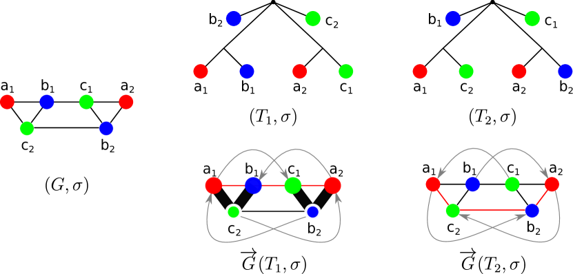
Figure 13: The $\mathsf{S}$-thin 3-RBMG $(G,\sigma)$ is explained by two trees $(T_{1},\sigma)$ and $(T_{2},\sigma)$ that induce distinct BMGs $\mathaccent 382{G}(T_{1},\sigma)$ and $\mathaccent 382{G}(T_{2},\sigma)$. In $\mathaccent 382{G}(T_{1},\sigma)$, $P^{1}=\langle a_{1}b_{1}c_{1}a_{2}\rangle$ defines a good quartet, while $P^{2}=\langle a_{1}c_{2}b_{2}a_{2}\rangle$ induces a bad quartet. In $\mathaccent 382{G}(T_{2},\sigma)$ the situation is reversed. Moreover, the quartets for $P^{1}$ and $P^{2}$ induce different leaf sets. Denoting the leaf colors “red”, “blue”, and “green” by $r$, $s$, and $t$, respectively, we obtain $L_{t}^{P^{1}}=\{a_{1},b_{1}\}$, $L_{s}^{P^{1}}=\{a_{2},c_{1}\}$, and $L_{*}^{P^{1}}=\{b_{2},c_{2}\}$, while $L_{s}^{P^{2}}=\{a_{1},c_{2}\}$, $L_{t}^{P^{2}}=\{a_{2},b_{2}\}$, and $L_{*}^{P^{2}}=\{b_{1}.c_{1}\}$. The good quartets in $\mathaccent 382{G}(T_{1},\sigma)$ and $\mathaccent 382{G}(T_{2},\sigma)$ are indicated by red edges. The induced paths $\langle a_{1}b_{1}c_{1}b_{2}\rangle$ and $\langle a_{2}c_{1}b_{1}c_{2}\rangle$ are examples of ugly quartets.

Lemma 32.

Let $(G,\sigma)$ be an RBMG, $Q$ a set of four vertices with three colors, $G[Q]\in\mathscr{P}_{4}$, and $(\mathaccent 382{G},\sigma)$ a BMG containing $(G,\sigma)$. Then $Q$ is either a good, a bad, or an ugly quartet.

Proof.

By Obs. 5, any induced $P_{4}$ is either of the form $\langle xyx^{\prime}z\rangle$ or $\langle xyzx^{\prime}\rangle$. In the first case $Q$ is an ugly quartet. For the remainder of the proof we thus assume $\langle xyzx^{\prime}\rangle$, and w.l.o.g, we suppose that the vertex colors are $\sigma(x)=\sigma(x^{\prime})=r$, $\sigma(y)=s$, and $\sigma(z)=t$.

Let $(T,\sigma)$ be a leaf-colored tree that explains $(\mathaccent 382{G},\sigma)$, and thus, by assumption, also $(G,\sigma)$. Since $\langle xyzx^{\prime}\rangle$ is an induced $P_{4}$ in $(G,\sigma)$, the edge $xz$ cannot be contained in $E(G)$. Hence, we are left with three cases: (i) $(x,z)\in E(\mathaccent 382{G})$ and $(z,x)\notin E(\mathaccent 382{G})$, (ii) $(z,x)\in E(\mathaccent 382{G})$ and $(x,z)\notin E(\mathaccent 382{G})$, and (iii) $(x,z),(z,x)\notin E(\mathaccent 382{G})$.

Case (i). We have $x^{\prime}\in N^{+}_{r}(z)$ and $x\notin N^{+}_{r}(z)$, i.e., $\operatorname{lca}_{T}(x^{\prime},z)\prec_{T}\operatorname{lca}_{T}(x,z)=:u$. This implies $\operatorname{lca}_{T}(x,x^{\prime})=u$. Moreover, $(x,y)\in E(G)$ implies $\operatorname{lca}_{T}(x,y)\preceq_{T}\operatorname{lca}_{T}(x^{\prime},y)$. In case of equality, we have $\operatorname{lca}_{T}(x,y)=\operatorname{lca}_{T}(x^{\prime},y)\succeq_{T}u$. Thus, $x\in N^{+}_{r}(y)$ implies $x^{\prime}\in N^{+}_{r}(y)$. Hence, since $x^{\prime}y\notin E(G)$, there must exist a leaf $y^{\prime}\in L[s]$ such that $\operatorname{lca}_{T}(x^{\prime},y^{\prime})\prec_{T}\operatorname{lca}_{T}(x^{\prime},y)$. Then, $\operatorname{lca}_{T}(x^{\prime},z)\prec_{T}u$ implies either $\operatorname{lca}_{T}(z,y^{\prime})\prec_{T}u\preceq_{T}\operatorname{lca}_{T}(x^{\prime},y)$ or $\operatorname{lca}_{T}(z,y^{\prime})=\operatorname{lca}_{T}(x^{\prime},y^{\prime})\prec_{T}\operatorname{lca}_{T}(x^{\prime},y)$. Either alternative contradicts $yz\in E(G)$. Therefore, $\operatorname{lca}_{T}(x,y)\prec_{T}\operatorname{lca}_{T}(x^{\prime},y)$. Together with $\operatorname{lca}_{T}(x,x^{\prime})=u$ this implies $\operatorname{lca}_{T}(x,y)\prec_{T}u$. Now let $u_{y}\succeq_{T}\operatorname{lca}_{T}(x,y)$ and $u_{z}\succeq_{T}\operatorname{lca}_{T}(x^{\prime},z)$, where $u_{y},u_{z}\in\mathsf{child}(u)$. Then, $yz\in E(G)$ implies that $t\notin\sigma(L(T(u_{y})))$ and $s\notin\sigma(L(T(u_{z})))$. Hence, $(x,z),(x^{\prime},y)\in E(\mathaccent 382{G})$ and $(z,x),(y,x^{\prime})\notin E(\mathaccent 382{G})$, i.e., $\{x,y,z,x^{\prime}\}$ forms a good quartet.

Case (ii). We have $x,x^{\prime}\in N^{+}_{r}(z)$, thus $u\coloneqq\operatorname{lca}_{T}(x,z)=\operatorname{lca}_{T}(x^{\prime},z)$. On the other hand, $(x,z)\notin E(\mathaccent 382{G})$ implies that there exists a leaf $z^{\prime}\in L[t]$ such that $\operatorname{lca}_{T}(x,z^{\prime})\prec_{T}\operatorname{lca}_{T}(x,z)$. Hence, as $z\in N^{+}_{t}(x^{\prime})$, we have distinct $u_{x},u_{x^{\prime}},u_{z}\in\mathsf{child}(u)$ such that $x,z^{\prime}\prec_{T}u_{x}$, $x^{\prime}\preceq_{T}u_{x^{\prime}}$, and $z\preceq_{T}u_{z}$. Moreover, $yz\in E(G)$ implies $\operatorname{lca}_{T}(y,z)\preceq_{T}\operatorname{lca}_{T}(y,z^{\prime})$, thus we either have (a) $\operatorname{lca}_{T}(y,z)\prec_{T}\operatorname{lca}_{T}(y,z^{\prime})$ or (b) $\operatorname{lca}_{T}(y,z)=\operatorname{lca}_{T}(y,z^{\prime})$. In both cases, we have $u_{x}\prec_{T}\operatorname{lca}(x,y)$, thus, since $xy\in E(G)$, it follows $s\notin\sigma(L(T(u_{x})))$. Similarly, since $zx^{\prime}\in E(G)$, we have $r\notin\sigma(L(T(u_{z})))$ and $t\notin\sigma(L(T(u_{x^{\prime}})))$. This in particular implies $\operatorname{lca}(x^{\prime},y)\preceq\operatorname{lca}(x,y)$. Moreover, as $x^{\prime}y\notin E(G)$, there must exist a leaf $y^{\prime}\in L[s]$ with $\operatorname{lca}_{T}(x^{\prime},y^{\prime})\prec_{T}\operatorname{lca}_{T}(x^{\prime},y)$. In Case (a), we have $y\in L(T(v_{z}))$ and thus $\operatorname{lca}_{T}(x^{\prime},y)=u$, which implies $y^{\prime}\preceq_{T}u_{x^{\prime}}$. In summary, this implies for Case (a) $x,z^{\prime}\prec_{T}u_{x}$, $x^{\prime},y^{\prime}\prec_{T}u_{x^{\prime}}$, and $y,z\prec_{T}u_{z}$ as well as $\sigma(L(T(u_{x})))=\{r,t\}$, $\sigma(L(T(u_{x^{\prime}})))=\{r,s\}$, and $\sigma(L(T(u_{z})))=\{s,t\}$. Hence, $(z,x),(y,x^{\prime})\in E(\mathaccent 382{G})$ and $(x,z),(x^{\prime},y)\notin E(\mathaccent 382{G})$, i.e., $\{x,y,z,x^{\prime}\}$ is a bad quartet in $(\mathaccent 382{G},\sigma)$. In Case (b), if $\operatorname{lca}_{T}(x^{\prime},y^{\prime})\succeq u$, then $\operatorname{lca}_{T}(x,y^{\prime})=\operatorname{lca}_{T}(x^{\prime},y^{\prime})\prec_{T}\operatorname{lca}_{T}(x^{\prime},y)$, contradicting $xy\in E(G)$. Hence, $y^{\prime}\preceq_{T}u_{x^{\prime}}$. This implies $\operatorname{lca}_{T}(x,y)=u$ since otherwise $\operatorname{lca}_{T}(x,y^{\prime})=u\prec_{T}\operatorname{lca}_{T}(x,y)$; again a contradiction to $xy\in E(G)$. Let $u_{y}\in\mathsf{child}(u)$ be such that $y\preceq_{T}u_{y}$. Since $xy,yz\in E(G)$, we conclude $\sigma(L(T(u_{y})))=\{s\}$. Moreover, $yz\in E(G)$ then implies $s\notin\sigma(L(T(u_{z})))$. Summarizing Case (b), we thus have $x,z^{\prime}\prec_{T}u_{x}$, $x^{\prime},y^{\prime}\prec_{T}u_{x^{\prime}}$, $y\preceq_{T}u_{y}$, and $z\prec_{T}u_{z}$ as well as $\sigma(L(T(u_{x})))=\{r,t\}$, $\sigma(L(T(u_{x^{\prime}})))=\{r,s\}$, $\sigma(L(T(u_{y})))=\{s\}$, and $\sigma(L(T(u_{z})))=\{t\}$. One now easily checks that $\{x,y,z,x^{\prime}\}$ again forms a bad quartet in $(\mathaccent 382{G},\sigma)$.

Case (iii). Let $u\coloneqq\operatorname{lca}_{T}(x,x^{\prime})$. Then $(x,z),(z,x)\notin E(\mathaccent 382{G})$ implies $\operatorname{lca}_{T}(x^{\prime},z)\prec_{T}\operatorname{lca}_{T}(x,z)$ and there must exist some leaf $z^{\prime}\in L[t]$ such that $\operatorname{lca}_{T}(x,z^{\prime})\prec_{T}\operatorname{lca}_{T}(x,z)$. Hence, there are $u_{x},u_{x^{\prime}}\in\mathsf{child}(u)$ with $\operatorname{lca}_{T}(x,z^{\prime})\preceq_{T}u_{x}$ and $\operatorname{lca}_{T}(x^{\prime},z)\preceq_{T}u_{x^{\prime}}$. By construction, we therefore have either $\operatorname{lca}_{T}(x,y)\prec_{T}\operatorname{lca}_{(}x^{\prime},y)$ or $\operatorname{lca}_{T}(x,y)=\operatorname{lca}_{(}x^{\prime},y)\succeq_{T}u$. The first case implies $\operatorname{lca}_{T}(y,z^{\prime})\prec_{T}u=\operatorname{lca}_{T}(y,z)$, which contradicts $yz\in E(G)$. Hence, it must hold $\operatorname{lca}_{T}(x,y)=\operatorname{lca}_{(}x^{\prime},y)\succeq_{T}u$ and thus, $x^{\prime}\in N_{r}^{+}(y)$ because $x\in N_{r}^{+}(y)$. Consequently, since $x^{\prime}y\notin E(G)$, there must be some $y^{\prime}\in L[s]$ such that $\operatorname{lca}_{T}(x^{\prime},y^{\prime})\prec_{T}\operatorname{lca}_{T}(x^{\prime},y)$. The same argumentation as in Case (i) shows that $\operatorname{lca}_{T}(x^{\prime},z)\prec_{T}u$ implies either $\operatorname{lca}_{T}(z,y^{\prime})\prec_{T}u\preceq_{T}\operatorname{lca}_{T}(x^{\prime},y)$ or $\operatorname{lca}_{T}(z,y^{\prime})=\operatorname{lca}_{T}(x^{\prime},y^{\prime})\prec_{T}\operatorname{lca}_{T}(x^{\prime},y)$, which in either case contradicts $yz\in E(G)$. We therefore conclude that Case (iii) is impossible.

∎

We immediately find the following result that links good quartets to 3-RBMGs of Type (B):

Lemma 33.

Let $(G,\sigma)$ be an undirected, connected, $\mathsf{S}$-thin and properly 3-colored graph that contains an induced path $P$ on four vertices. If $(G,\sigma)$ satisfies (B1) to (B4.b) w.r.t. $P$, then there exists a tree $(T,\sigma)$ explaining $(G,\sigma)$ such that $P$ is a good quartet in $\mathaccent 382{G}(T,\sigma)$.

Proof.

Suppose that $(G,\sigma)$ satisfies (B1) to (B4.b) w.r.t. $P$. Then, by Lemma 25, $(G,\sigma)$ is a 3-RBMG of Type (B). Thus, according to Lemma 24, there exists a Type (II^∗) tree $(T,\sigma)$ with root $\rho_{T}$ such that $L_{t}^{P}=L(T(v_{1}))$, $L_{s}^{P}=L(T(v_{2}))$ for distinct $v_{1},v_{2}\in\mathsf{child}_{T}(\rho_{T})\setminus L$ and $L_{*}^{P}=\mathsf{child}_{T}(\rho_{T})\cap L$, that explains $(G,\sigma)$. In particular, by Property (B1), we have $P\coloneqq\langle xyzx^{\prime}\rangle$ with $\sigma(x)=\sigma(x^{\prime})=r$, $\sigma(y)=s$ and $\sigma(z)=t$ for distinct colors $r,s,t$. Now, as $x,y\in L_{t}^{P}$ and $x^{\prime},z\in L_{s}^{P}$ by Lemma 25 and, by definition, $\sigma(L_{t}^{P})=\{r,s\}$, $\sigma(L_{s}^{P})=\{r,t\}$, one easily checks that $P$ is indeed a good quartet in $\mathaccent 382{G}(T,\sigma)$. ∎

We continue with some basic result about ugly quartets before analyzing good and bad quartets in more details.

Lemma 34.

Let $\langle xyx^{\prime}z\rangle$ be an ugly quartet in some connected $\mathsf{S}$-thin 3-RBMG $(G,\sigma)$ and $(T,\sigma)$ with root $\rho_{T}$ a tree of Type (II) or (III) that explains $(G,\sigma)$. Then the children $v_{a}\in\mathsf{child}(\rho_{T})$ with $a\in\{x,x^{\prime},y,z\}$ and $a\preceq_{T}v_{a}$ satisfy exactly one of the following conditions:

1. $v_{x}=x$, $v_{x^{\prime}}=v_{z}$, $v_{y}\neq y$, and $v_{x}$, $v_{y}$, $v_{z}$ are pairwise distinct,

2. $v_{x}=v_{x^{\prime}}=v_{z}\neq v_{y}$ and $v_{y}\neq y$,

3. $v_{x}\neq x$, $v_{x^{\prime}}=x^{\prime}$, $v_{y}=v_{z}$, and $v_{x}$, $v_{x^{\prime}}$, $v_{y}$ are pairwise distinct,

4. $v_{x}\neq x$, $v_{x^{\prime}}=x^{\prime}$, $v_{y}\neq y$, $v_{z}=z$, and $v_{x}$, $v_{x^{\prime}}$, $v_{y}$, $v_{z}$ are pairwise distinct,

5. $v_{x}\neq x$, $v_{x^{\prime}}=x^{\prime}$, $v_{y}=y$, $v_{z}\neq z$, and $v_{x}$, $v_{x^{\prime}}$, $v_{y}$, $v_{z}$ are pairwise distinct.

In particular, $x$, $x^{\prime}$, and $y$ can never reside within the same subtree $T(v_{x})$. Indeed, all cases may appear.

Proof.

Let $L$ be the vertex set of $G$ and $r,s,t$ be three distinct colors in $(G,\sigma)$, where $\sigma(x)=\sigma(x^{\prime})=r$, $\sigma(y)=s$, and $\sigma(z)=t$.

We start by considering the two Cases (a) $v_{x}=x$, i.e., $x\in\mathsf{child}(\rho_{T})$ and (b) $v_{x}\neq x$.

We first assume Case (a), i.e., $x\in\mathsf{child}(\rho_{T})$. Note first that this immediately implies $x^{\prime}\notin\mathsf{child}(\rho_{T})$, i.e., $v_{x^{\prime}}\neq x^{\prime}$ because $(G,\sigma)$ is $\mathsf{S}$-thin (cf. Lemma 18). Moreover, we have $s\notin\sigma(L(T(v_{x^{\prime}})))$ because $x^{\prime}y\in E(G)$ and thus, since $v_{x^{\prime}}\neq x^{\prime}$, Lemma 8 implies that $t\in\sigma(L(T(v_{x^{\prime}})))$. Consequently, $z\in L(T(v_{x^{\prime}}))$ as otherwise, there is some $z^{\prime}\in L(T(v_{x^{\prime}}))$ such that $\operatorname{lca}(x^{\prime},z^{\prime})\prec_{T}\operatorname{lca}(x^{\prime},z)$, which contradicts $x^{\prime}z\in E(G)$. Since $xy\in E(G)$, $x\in\mathsf{child}(\rho_{T})$ implies either $y\in\mathsf{child}(\rho_{T})$ or $\sigma(L(T(v_{y})))=\{s,t\}$ as otherwise $\operatorname{lca}(x^{\prime\prime},y)\prec_{T}\operatorname{lca}(x,y)$ for some $x^{\prime\prime}\in L(T(v_{y}))\cap L[r]$, contradicting $xy\in E(G)$. If the first case is true, we have, by construction, $\operatorname{lca}(y,z)\preceq_{T}\operatorname{lca}(y,z^{\prime})$ and $\operatorname{lca}(y,z)\preceq_{T}\operatorname{lca}(y^{\prime},z)$ for any $y^{\prime}\in L[s]$ and $z^{\prime}\in L[t]$, i.e., $yz\in E(G)$; a contradiction since $\langle xyx^{\prime}z\rangle$ is an induced $P_{4}$. Hence, we have $\sigma(L(T(v_{y})))=\{s,t\}$, which in particular implies $v_{y}\neq y$ and $v_{y}\neq v_{x^{\prime}},v_{x}$. Using Lemma 19, one easily checks that, if $\mathsf{par}(x^{\prime})=\mathsf{par}(z)$, $\langle xyx^{\prime}z\rangle$ is indeed an induced $P_{4}$ in $(G,\sigma)$, which finally shows Statement (i).

Now assume that Case (b) is true, i.e., $v_{x}\neq x$. Then, by Lemma 8, the subtree $(T(v_{x}),\sigma_{|L(T(v_{x}))})$ must contain at least two colors. Assume first, for contradiction, that $s\in\sigma(L(T(v_{x})))$. Then, as $xy,x^{\prime}y\in E(G)$, Lemma 19 implies that $x^{\prime}\in L(T(v_{x}))$ and $\mathsf{par}(x)=\mathsf{par}(x^{\prime})=\mathsf{par}(y)$, which contradicts the $\mathsf{S}$-thinness of $(G,\sigma)$. Hence, $\sigma(L(T(v_{x})))=\{r,t\}$, and in particular $v_{x}\neq v_{y}$.
If $v_{x}=v_{x^{\prime}}$, it follows from $x^{\prime}z\in E(G)$ that $z\preceq_{T}v_{x}$ (cf. Lemma 19), i.e., $v_{x}=v_{z}$. Moreover, since $s\notin\sigma(L(T(v_{x})))$ and $yz\notin E(G)$, Lemma 19(iv) implies $v_{y}\neq y$. Hence, by Lemma 8, it must hold $\sigma(L(T(v_{y})))=\{s,t\}$. Choosing $\mathsf{par}(x^{\prime})=\mathsf{par}(z)\neq\mathsf{par}(x)$, one can again use Lemma 19 in order to show that $\langle xyx^{\prime}z\rangle$ forms an induced $P_{4}$, which proves (ii).
On the other hand, if $v_{x}\neq v_{x^{\prime}}$, then $xy,x^{\prime}y\in E(G)$ requires $\operatorname{lca}(x,y)=\operatorname{lca}(x^{\prime},y)$, hence $v_{y}\neq v_{x},v_{x^{\prime}}$. Again, $x^{\prime}y\in E(G)$ then implies $s\notin\sigma(L(T(v_{x^{\prime}})))$. Since $\sigma(L(T(v_{x^{\prime}})))=\sigma(L(T(v_{x})))=\{r,t\}$ is not possible by construction of a tree of Type (II) or (III) contains only color $r$, hence $v_{x^{\prime}}=x^{\prime}$ by Lemma 8. It finally remains to distinguish the two cases $v_{y}=v_{z}$ and $v_{y}\neq v_{z}$. In the first case, if $\mathsf{par}(y)\neq\mathsf{par}(z)$ in $(T,\sigma)$, we can apply Lemma 19 to show $yz\notin E(G)$ and furthermore, that $\langle xyx^{\prime}z\rangle$ is again an induced $P_{4}$. This yields Statement (iii).
If the latter case is true, i.e., $v_{y}\neq v_{z}$, then, as $xy,x^{\prime}y,x^{\prime}z\in E(G)$, we have in particular $r\notin\sigma(L(T(v_{y}))),\sigma(L(T(v_{z})))$. Furthermore, since $yz\notin E(G)$, there is either some $z^{\prime}\in L(T(v_{y}))\cap L[t]$ such that $\operatorname{lca}(y,z^{\prime})\prec_{T}\operatorname{lca}(y,z)$, or some $y^{\prime}\in L(T(v_{z}))\cap L[s]$ such that $\operatorname{lca}(y^{\prime},z)\prec_{T}\operatorname{lca}(y,z)$. Note that, since $v_{y}\neq v_{z}$, $\sigma(L(T(v_{y})))=\sigma(L(T(v_{z})))=\{s,t\}$ is not possible by construction of $(T,\sigma)$. Hence, by applying Lemma 8 to these two cases, we either obtain (iv) or (v). Again, Lemma 19 easily shows that $\langle xyx^{\prime}z\rangle$ is an induced $P_{4}$ in $(G,\sigma)$, which concludes the proof. ∎

We will from now on focus on good and bad quartets only as they are of particular interest for the characterization of Type (B) 3-RBMGs. We start with some basic result.

Lemma 35.

Let $(G,\sigma)$ be an RBMG and $\color[rgb]{0,0,0}P\coloneqq\langle xyzx^{\prime}\rangle$ an induced $P_{4}$ in $(G,\sigma)$ with $\sigma(x)=\sigma(x^{\prime})$, let $(T,\sigma)$ be a tree explaining $(G,\sigma)$ and let $v\coloneqq\operatorname{lca}_{T}(x,x^{\prime},y,z)$. Then the distinct children $v_{i}\in\mathsf{child}(v)$ satisfy exactly one of the three alternatives

1. $x,y\preceq_{T}v_{1}$ and $x^{\prime},z\preceq_{T}v_{2}$,

2. $x\preceq_{T}v_{1}$, $y,z\preceq_{T}v_{2}$, and $x^{\prime}\preceq_{T}v_{3}$,

3. $x\preceq_{T}v_{1}$, $y\preceq_{T}v_{2}$, $x^{\prime}\preceq_{T}v_{3}$, and $z\preceq_{T}v_{4}$.

Indeed, all three cases may appear.

Proof.

Let $\sigma(x)=\sigma(x^{\prime})=r$, $\sigma(y)=s$, and $\sigma(z)=t$.
Suppose first $x,y\in L(T(v_{1}))$ for some $v_{1}\in\mathsf{child}(v)$. If $z\preceq_{T}v_{1}$, then $x^{\prime}\in L(T(v_{1}))$ since otherwise $\operatorname{lca}_{T}(x,z)\prec_{T}\operatorname{lca}_{T}(x^{\prime},z)$, contradicting $zx^{\prime}\in E(G)$. Thus, $\operatorname{lca}_{T}(x,x^{\prime},y,z)\prec_{T}v$; a contradiction to the definition of $v$. Hence, $z\notin L(T(v_{1}))$. Then, $yz\in E(G)$ implies that $t\notin\sigma(L(T(v_{1})))$, hence in particular $v=\operatorname{lca}_{T}(x,z)\preceq_{T}\operatorname{lca}_{T}(x,z^{\prime})$ for any $z^{\prime}\in L[t]$, i.e., $z\in N^{+}_{t}(x)$. Since $xz\notin E(G)$, it must therefore hold $\operatorname{lca}_{T}(x^{\prime},z)\prec_{T}\operatorname{lca}_{T}(x,z)=v$, thus $x^{\prime},z\in L(T(v_{2}))$ for some $v_{2}\in\mathsf{child}(v)\setminus\{v_{1}\}$. This implies Case (i).

Now suppose $x$ and $y$ are located in different subtrees below $v$, i.e., $x\preceq_{T}v_{1}$ and $y\preceq_{T}v_{2}$ for distinct children $v_{1},v_{2}\in\mathsf{child}(v)$. Since $xy\in E(G)$ and $\operatorname{lca}_{T}(x,y)=v$, we conclude that $r\notin\sigma(L(T(v_{2})))$ and $s\notin\sigma(L(T(v_{1})))$. This immediately implies $x^{\prime}\notin L(T(v_{1}))$ as otherwise (a) $\operatorname{lca}_{T}(x,y)=\operatorname{lca}_{T}(x^{\prime},y)$ results in $x^{\prime}\in N^{+}_{r}(y)$, and (b) $\operatorname{lca}_{T}(x^{\prime},y)\preceq_{T}\operatorname{lca}_{T}(x^{\prime},y^{\prime})$ for any $y^{\prime}\in L[s]$, hence $x^{\prime}y\in E(G)$; a contradiction. Therefore, there must be a child $v_{3}\neq v_{1},v_{2}$ of $v$ such that $x^{\prime}\preceq_{T}v_{3}$. As a consequence, $z$ cannot be contained in $L(T(v_{1}))$ since this would imply $\operatorname{lca}_{T}(x,z)\prec_{T}\operatorname{lca}_{T}(x^{\prime},z)$, contradicting $x^{\prime}z\in E(G)$. Suppose $z\in L(T(v_{3}))$. Then, since $yz\in E(G)$, we have $t\notin\sigma(L(T(v_{2})))$ and $s\notin\sigma(L(T(v_{3})))$. As we already know $r\notin\sigma(L(T(v_{2})))$, we conclude $\sigma(L(T(v_{2})))=\{s\}$ and $\sigma(L(T(v_{3})))=\{r,t\}$. Clearly, this implies $yx^{\prime}\in E(G)$; a contradiction. Therefore, $z\notin L(T(v_{3}))$, thus we either have $z\preceq_{T}v_{2}$ or there exists another child $v_{4}$ of $v$ ($v_{4}\neq v_{1},v_{2},v_{3}$) such that $z\preceq_{T}v_{4}$. The latter shows that one of the Cases (ii) and (iii) may occur. However, we need to ensure that both can happen given the existence of the induced $P_{4}$ $\langle xyzx^{\prime}\rangle$. Let us first assume $z\in L(T(v_{2}))$, thus $\sigma(L(T(v_{2})))=\{s,t\}$. If $\sigma(L(T(v_{1})))=\{r,t\}$ and $\sigma(L(T(v_{3})))=\{r,s\}$, then one easily checks that $\langle xyzx^{\prime}\rangle$ is an induced $P_{4}$ in $(G,\sigma)$, which implies statement (ii). On the other hand, if $z\preceq_{T}v_{4}$ and $\sigma(L(T(v_{1})))=\{r,t\}$, $\sigma(L(T(v_{2})))=\{s\}$, $\sigma(L(T(v_{3})))=\{r,s\}$ $\sigma(L(T(v_{4})))=\{t\}$, then $\langle xyzx^{\prime}\rangle$ also forms an induced $P_{4}$ in $(G,\sigma)$, i.e., Case (iii) is true. ∎

It turns out that the location of good quartets in any tree is strictly constrained:

Lemma 36.

Let $(\mathaccent 382{G},\sigma)$ be a BMG containing a good quartet $\langle xyzx^{\prime}\rangle$, $(T,\sigma)$ a tree explaining $(\mathaccent 382{G},\sigma)$ and $v\coloneqq\operatorname{lca}(x,x^{\prime},y,z)$. Then, $x,y\preceq_{T}v_{1}$ and $x^{\prime},z\preceq_{T}v_{2}$ for some distinct $v_{1},v_{2}\in\mathsf{child}(v)$.

Proof.

Let $v\coloneqq\operatorname{lca}_{T}(x,x^{\prime},y,z)$ and $v_{1}\in\mathsf{child}(v)$ such that $x\preceq_{T}v_{1}$. Suppose first $y\notin L(T(v_{1}))$, hence in particular $\operatorname{lca}_{T}(y,x^{\prime})\preceq_{T}\color[rgb]{0,0,0}v=\operatorname{lca}_{T}(y,x)$. Since $xy\in E(G(T,\sigma))$, this implies $x^{\prime}\in N^{+}_{\sigma(x)}(y)$ in $(\mathaccent 382{G},\sigma)$; a contradiction to $\langle xyzx^{\prime}\rangle$ forming a good quartet. Hence, $y\preceq_{T}v_{1}$. As $(T,\sigma)$ must satisfy one of the three cases of Lemma 35 and the only possible case is (i), we can now conclude $x,y\preceq_{T}v_{1}$ and $x^{\prime},z\preceq_{T}v_{2}$.

∎

Note that the latter result in addition shows that the Cases (ii) and (iii) in Lemma 35 must correspond to bad quartets. Lemma 36 now can be used to show that the any good quartet in an BMG is endowed with the same coloring.

Corollary 8.

Let $(G,\sigma)$ be a connected $\mathsf{S}$-thin 3-RBMG of Type (B), $(\mathaccent 382{G},\sigma)$ a BMG containing $(G,\sigma)$ as symmetric part, and let $Q=\langle xyzx^{\prime}\rangle$ with $\sigma(x)=\sigma(x^{\prime})$ be a good quartet in $(\mathaccent 382{G},\sigma)$. Then every good quartet with $\langle x_{1}y_{1}z_{1}x_{1}^{\prime}\rangle\in\mathscr{P}_{4}$ has colors $\sigma(x_{1})=\sigma(x_{1}^{\prime})=\sigma(x)$, $\sigma(y_{1})=\sigma(y)$, and $\sigma(z_{1})=\sigma(z)$.

Proof.

Since $(G,\sigma)$ a of Type (B), any leaf-colored tree $(T,\sigma)$ with root $\rho_{T}$ explaining $(G,\sigma)$ is of Type (II) (cf. Theorem 4). Hence, there are distinct $v_{1},v_{2}\in\mathsf{child}(\rho_{T})$ with $|\sigma(L(T(v_{1})))|=|\sigma(L(T(v_{2})))|=2$ and $\mathsf{child}(\rho_{T})\setminus\{v_{1},v_{2}\}\subset L$. By Lemma 36, we have $x,y\preceq_{T}v_{1}$ and $x^{\prime},z\preceq_{T}v_{2}$, hence $\sigma(L(T(v_{1})))=\{\sigma(x),\sigma(y)\}$ and $\sigma(L(T(v_{2})))=\{\sigma(x),\sigma(z)\}$. Therefore, the statement follows directly from Lemma 36.

∎

We are now in the position to formulate one of the main results of this section:

Lemma 37.

Let $(G,\sigma)$ be a connected $\mathsf{S}$-thin 3-RBMG of Type (B) and $(\mathaccent 382{G},\sigma)$ a BMG containing $(G,\sigma)$ as its symmetric part. Moreover, let $L_{s}^{Q}$, $L_{t}^{Q}$, and $L_{*}^{Q}$ be defined w.r.t. a good quartet $Q\coloneqq\langle x_{1}y_{1}z_{1}x_{1}^{\prime}\rangle$ where $x_{1},x_{1}^{\prime}\in L[r]$, $y_{1}\in L[s]$, and $z_{1}\in L[t]$ for distinct colors $r,s,t$. Then, for any good quartet $Q^{\prime}$, it holds $L_{s}^{Q^{\prime}}=L_{s}^{Q}$, $L_{t}^{Q^{\prime}}=L_{t}^{Q}$, and $L_{*}^{Q^{\prime}}=L_{*}^{Q}$.

Proof.

Let $(T,\sigma)$ with root $\rho_{T}$ be a leaf-colored tree that explains $(\mathaccent 382{G},\sigma)$ and thus, also $(G,\sigma)$. Since $(G,\sigma)$ is of Type (B), we can choose $(T,\sigma)$ to be of Type (II) by Theorem 4, i.e., there are distinct children $v_{1},v_{2}\in\mathsf{child}(\rho_{T})$ with $|\sigma(L(T(v_{1})))|=|\sigma(L(T(v_{2})))|=2$ such that these two subtrees have exactly one color in common, and $\mathsf{child}(\rho_{T})\setminus\{v_{1},v_{2}\}\subset L$. Applying Lemma 24, we can choose $(T,\sigma)$ such that it is of Type (II^∗) and satisfies $L_{t}^{Q}=L(T(v_{1}))$, $L_{s}^{Q}=L(T(v_{2}))$ and $L_{*}^{Q}=\mathsf{child}(\rho_{T})\cap L$. On the other hand, Lemma 36 implies $x_{1},y_{1}\preceq_{T}v_{1}$ and $x_{1}^{\prime},z_{1}\preceq_{T}v_{2}$.

Now let $Q^{\prime}\coloneqq\langle x_{2}y_{2}z_{2}x_{2}^{\prime}\rangle\neq Q$ be another good quartet in $(\mathaccent 382{G},\sigma)$. By Cor. 8, we have $x_{2},x_{2}^{\prime}\in L[r]$, $y_{2}\in L[s]$ and $z_{2}\in L[t]$. Lemma 36 and the structure of Type (II) trees then imply $x_{2},y_{2}\preceq_{T}v_{1}$ and $x_{2}^{\prime},z_{2}\preceq_{T}v_{2}$. Consider first $L_{t}^{Q^{\prime}}$ and let $x\in L[r],y\in L[s]$. Then, by definition, $y\in L_{t}^{Q^{\prime}}$ if and only if $\langle x^{\prime}yz_{2}\rangle\in\mathscr{P}_{3}$ for each $x^{\prime}\in N_{r}(y)$. Since any two leaves of color $s$ and $t$ are reciprocal best matches in $(G,\sigma)$ by Lemma 19(iii) and $x^{\prime}z_{2}\notin E(G)$ for any $x^{\prime}\in N_{r}(y)$ only if $x^{\prime}\notin L(T(v_{2}))$ by cf. Lemma 19(i)+(iv), we have $\langle x^{\prime}yz_{2}\rangle\in\mathscr{P}_{3}$ for any $x^{\prime}\in N_{r}(y)$ if and only if $\langle x^{\prime}yz_{1}\rangle\in\mathscr{P}_{3}$ for any $x^{\prime}\in N_{r}(y)$. Hence, $y\in L_{t}^{Q^{\prime}}$ if and only if $y\in L_{t}^{Q}$, i.e., $L_{t}^{Q}\cap L[s]=L_{t}^{Q^{\prime}}\cap L[s]$. If $N_{s}(x)=\emptyset$, the latter by definition of $L_{t}^{Q}$ immediately implies that $x\in L_{t}^{Q^{\prime}}$ if and only if $x\in L_{t}^{Q}$. On the other hand, if $N_{s}(x)\neq\emptyset$, then $x\in L_{t}^{Q^{\prime}}$ if and only if $N_{r}(y^{\prime})=\{x\}$ for some induced $P_{3}$ $\langle xy^{\prime}z_{2}\rangle$. This can only be true if $y^{\prime}\in L(T(v_{1}))$ since otherwise, $y^{\prime}z_{2}x_{2}^{\prime}$ forms a circle, thus $|N_{r}(y^{\prime})|>1$. Consequently, $x\in L(T(v_{1}))$ by Lemma 19(i). Since $y^{\prime}z^{\prime}\in E(G)$ for any $y^{\prime}\in L[s],z^{\prime}\in L[t]$ by Lemma 19(ii) and $x^{\prime}z\notin E(G)$ for any $z\in L(T(v_{2}))\cap L[t]$ by Lemma 19(ii), we conclude that $\langle xy^{\prime}z_{2}\rangle$ is an induced $P_{3}$ with $N_{r}(y^{\prime})=\{x\}$ if and only if $\langle xy^{\prime}z_{1}\rangle$ is an induced $P_{3}$ with $N_{r}(y^{\prime})=\{x\}$, hence $L_{t}^{Q}\cap L[r]=L_{t}^{Q^{\prime}}\cap L[r]$. We therefore conclude $L_{t}^{Q}=L_{t}^{Q^{\prime}}$.

By symmetry, an analogous argument shows $L_{s}^{Q}=L_{s}^{Q^{\prime}}$. Together, this finally implies $L_{*}^{Q}=L_{*}^{Q^{\prime}}$, completing the proof. ∎

Fig. 13 shows that good and bad quartets do not necessarily imply the same leaf sets $L_{s}^{P}$, $L_{t}^{P}$.

We simplify the notation using the following abbreviations:

Definition 18.

$(G_{rst},\sigma_{rst})\coloneqq(G[L[r]\cup L[s]\cup L[t]],\sigma_{|L[r]\cup L[s]\cup L[t]})$ and $(T_{rst},\sigma_{rst})\coloneqq(T_{|L[r]\cup L[s]\cup L[t]},\sigma_{|L[r]\cup L[s]\cup L[t]})$ for any three colors $r,s,t\in S$.

The restriction of a BMG $\mathaccent 382{G}(T,\sigma)$ to a subset $S^{\prime}\subset S$ of colors is an induced subgraph of $\mathaccent 382{G}(T,\sigma)$ explained by the restriction of $(T,\sigma)$ to the leaves with colors in $S^{\prime}$, and thus again a BMG [Geiß et al., 2019b, Observation 1]. Since $G(T,\sigma)$ is the symmetric part of $\mathaccent 382{G}(T,\sigma)$, it inherits this property. In particular, we have

Observation 6.

If $(G,\sigma)$ is an $n$-RBMG, $n\geq 3$ explained by $(T,\sigma)$, then for any three colors $r,s,t\in S$, the restricted tree $(T_{rst},\sigma_{rst})$ explains $(G_{rst},\sigma_{rst})$, and $(G_{rst},\sigma_{rst})$ is an induced subgraph of $(G,\sigma)$.

This observation will play an important role in the proof of the following lemma as well as in Section F.

Lemma 38.

Let $(\mathaccent 382{G},\sigma)$ be a BMG. Then, the symmetric part $(G,\sigma)$ contains an induced 3-colored $P_{4}$ whose endpoints have the same color if and only if $(\mathaccent 382{G},\sigma)$ contains a good quartet.

Proof.

Note that, if $(\mathaccent 382{G},\sigma)$ contains a good quartet, then its symmetric part $(G,\sigma)$ by definition contains a 3-colored $P_{4}$ $\langle abcd\rangle$ with $\sigma(a)=\sigma(d)$.

Conversely, suppose that $(G,\sigma)$ contains a 3-colored induced $P_{4}$ $\langle abcd\rangle$ whose endpoints have the same color $\sigma(a)=\sigma(d)$. Moreover, let $S$ be the color set of $(G,\sigma)$ and $(T,\sigma)$ be a tree explaining $(\mathaccent 382{G},\sigma)$ and thus also $(G,\sigma)$. W.l.o.g. we can assume that the three colors of $\langle abcd\rangle$ are $r,s,t\in S$ without explicitly stating the particular coloring of the vertices $a,b,c,$ and $d$. By definition, $(G_{rst},\sigma_{rst})$ contains the induced path $\langle abcd\rangle$. W.l.o.g. we may assume that $(G_{rst},\sigma_{rst})$ is connected; otherwise the proof works analogously for the connected component of $(G_{rst},\sigma_{rst})$ that contains $\langle abcd\rangle$.

Let us first assume that $(G_{rst},\sigma_{rst})$ is $\mathsf{S}$-thin. In this case, we can apply Theorem 4 and conclude that $(G_{rst},\sigma_{rst})$ is either of Type (B) or (C), i.e., the restricted tree $(T_{rst},\sigma_{rst})$ with root $\rho\coloneqq\operatorname{lca}_{T}(L[r]\cup L[s]\cup L[t])$ that explains $(G_{rst},\sigma_{rst})$ must be of Type (II) or (III). Hence, there are distinct children $v_{1},v_{2}\in\mathsf{child}(\rho)$ with $\sigma(L(T_{rst}(v_{1})))=\{r,s\}$ and $\sigma(L(T_{rst}(v_{2})))=\{r,t\}$ for distinct colors $r,s,t$ (up to permutation of the colors). Then there exist leaves $x,y\in L(T_{rst}(v_{1}))$ and $x^{\prime},z\in L(T_{rst}(v_{2}))$ with $x,x^{\prime}\in L[r]$, $y\in L[s]$, and $z\in L[t]$ such that $xy,x^{\prime}z\in E(G_{rst})$ (cf. Lemma 10). Moreover, Lemma 19(ii) implies that $yz\in E(G_{rst})$ as well as $xz,x^{\prime}y\notin E(G_{rst})$. Hence, $\langle xyzx^{\prime}\rangle$ is an induced $P_{4}$ in $(G_{rst},\sigma_{rst})$ and thus, by Obs. 6, also in $(G,\sigma)$. Since $t\notin\sigma(L(T(v_{1})))$, we have $\rho=\operatorname{lca}_{T}(x,z)\preceq_{T}\operatorname{lca}_{T}(x,z^{\prime})$ for any $z^{\prime}\in L[t]$, i.e., $z\in N_{t}^{+}(x)$ in $(T,\sigma)$. In particular, $xz\notin E(G)$ then immediately implies $x\notin N_{r}^{+}(z)$. One similarly argues that $y\in N_{s}^{+}(x^{\prime})$ and $x^{\prime}\notin N_{r}^{+}(y)$ in $(T,\sigma)$, hence $(x,z),(x^{\prime},y)\in E(\mathaccent 382{G})$ and $(z,x),(y,x^{\prime})\notin E(\mathaccent 382{G})$. Therefore, $\langle xyzx^{\prime}\rangle$ is a good quartet in $(\mathaccent 382{G},\sigma)$.

Now, suppose that $(G_{rst},\sigma_{rst})$ is not $\mathsf{S}$-thin. In this case, we apply the same arguments as above to the quotient graph $(G_{rst}/\mathsf{S},\sigma_{rst}/\mathsf{S})$ and conclude that there exists a good quartet $\langle[a][b][c][d]\rangle$ induced by the tree $(T_{rst},\sigma_{rst})$ that explains $(G_{rst}/\mathsf{S},\sigma_{rst}/\mathsf{S})$. Let $x\in[a],y\in[b],z\in[c]$ and $x^{\prime}\in[d]$. Lemma 5 implies that $\langle xyzx^{\prime}\rangle$ is an induced $P_{4}$ with $\sigma(x)=\sigma(x^{\prime})$ in $(G_{rst},\sigma_{rst})$ and thus, by Obs. 6, also in $(G,\sigma)$. To conclude that $\langle xyzx^{\prime}\rangle$ is a good quartet it remains to show that $(x,z),(x^{\prime},y)\in E(\mathaccent 382{G})$ and $(z,x),(y,x^{\prime})\notin E(\mathaccent 382{G})$. In order to see this, observe first that $([a],[c]),([d],[b])\in E(\mathaccent 382{G}(T_{rst},\sigma_{rst}))$ and $([c],[a]),([b],[d])\notin E(\mathaccent 382{G}(T_{rst},\sigma_{rst}))$ since $\langle[a][b][c][d]\rangle$ is a good quartet induced by $(T_{rst},\sigma_{rst})$. To obtain a tree $(\hat{T},\hat{\sigma})$ that explains $(G_{rst},\sigma_{rst})$, we can proceed as in the proof of the “if-direction” in Lemma 7 and simply replace all edges $\mathsf{par}([v])[v]$ in $T_{rst}$ by edges $\mathsf{par}([v])v^{\prime}$ for all $v^{\prime}\in[v]$ and putting $\hat{\sigma}(v^{\prime})=\sigma_{rst}([v])$. Clearly, the latter construction and $([a],[c]),([d],[b])\in E(\mathaccent 382{G}(T_{rst},\sigma_{rst}))$ and $([c],[a]),([b],[d])\notin E(\mathaccent 382{G}(T_{rst},\sigma_{rst}))$ implies that $(x,z),(x^{\prime},y)\in E(\mathaccent 382{G}(\hat{T},\hat{\sigma}))$ and $(z,x),(y,x^{\prime})\notin E(\mathaccent 382{G}(\hat{T},\hat{\sigma}))$. Therefore, $\langle xyzx^{\prime}\rangle$ is a good quartet induced by $(\hat{T},\hat{\sigma})$ and thus, in $(G_{rst},\sigma_{rst})$. Now, by Obs. 6 implies that $\langle xyzx^{\prime}\rangle$ is a good quartet in $(\mathaccent 382{G},\sigma)$. ∎

Since every bad quartet induces in particular an induced $P_{4}$ with endpoints of the same color, Lemma 38 immediately implies:

Corollary 9.

If a BMG $(\mathaccent 382{G},\sigma)$ contains a bad quartet, then it contains a good quartet. In particular, any BMG $(\mathaccent 382{G},\sigma)$ whose symmetric part contains a 3-RBMG of Type (B) or (C) as induced subgraph, contains a good quartet.

Proof.

The first statement is an immediate consequence of Lemma 38. If $(G,\sigma)$ is a 3-RBMG of Type (B), then, by definition, it contains an induced $P_{4}$ of the form $(r,s,t,r)$ for distinct colors $r,s,t$. Hence, by Lemma 32, this $P_{4}$ is either a good or a bad quartet in $(\mathaccent 382{G},\sigma)$, where $(\mathaccent 382{G},\sigma)$ is a BMG whose symmetric part contains $(G,\sigma)$ as induced subgraph. Lemma 38 thus implies that $(\mathaccent 382{G},\sigma)$ contains a good quartet. If $(G,\sigma)$ is a 3-RBMG of Type (C), it must, by definition, contain an induced $C_{6}$ of the form $(r,s,t,r,s,t)$. In particular, it contains an induced $P_{4}$ whose endpoints are of the same color, thus we can again apply the same argumentation to complete the proof. ∎

The converse of Cor. 9 is, however, not true. As an example, consider the tree $T=((x,y),(x^{\prime}z))$ in Newick format with $\sigma(x)=\sigma(x^{\prime})=r$, $\sigma(y)=s$, $\sigma(z)=t$. The graph $G(T,\sigma)$ is the $P_{4}$ $\langle xyzx^{\prime}\rangle$, which is of course uniquely defined. The BMG $\mathaccent 382{G}(T,\sigma)$ contains the directed edges $(x,z),(x^{\prime},y)$ but not $(z,x),(y,x^{\prime})$, hence $Q=\{x,y,z,x^{\prime}\}=V(T)$ is a good quartet.

We close this section with a variation of Lemma 36 for Type (C) RBMGs:

Lemma 39.

Let $(G,\sigma)$ be a connected $\mathsf{S}$-thin 3-RBMG of Type (C) that contains an induced hexagon $H\coloneqq\langle x_{1}y_{1}z_{1}x_{2}y_{2}z_{2}\rangle$ with $|N_{t}(x_{1})|>1$, where $x_{i}\in L[r],y_{i}\in L[s],z_{i}\in L[t]$ for distinct colors $r,s,t$. Moreover, let $(T,\sigma)$ explain $(G,\sigma)$ and $v\coloneqq\operatorname{lca}_{T}(x_{1},x_{2},y_{1},y_{2},z_{1},z_{2})$. Then,

• $\langle x_{1}y_{1}z_{1}x_{2}\rangle$, $\langle z_{1}x_{2}y_{2}z_{2}\rangle$, and $\langle y_{2}z_{2}x_{1}y_{1}\rangle$ are good quartets in $\mathaccent 382{G}(T,\sigma)$,

• $\langle y_{1}z_{1}x_{2}y_{2}\rangle$, $\langle x_{2}y_{2}z_{2}x_{1}\rangle$, and $\langle z_{2}x_{1}y_{1}z_{1}\rangle$ are bad quartets in $\mathaccent 382{G}(T,\sigma)$, and

• $x_{1},y_{1}\preceq_{T}v_{1}$, $x_{2},z_{1}\preceq_{T}v_{2}$, and $y_{2},z_{2}\preceq_{T}v_{3}$ for some distinct $v_{1},v_{2},v_{3}\in\mathsf{child}_{T}(v)$.

Proof.

We start with proving Properties (i) and (ii). By definition and Lemma 32, $\langle x_{1}y_{1}z_{1}x_{2}\rangle$ is either a good or a bad quartet in $\mathaccent 382{G}(T,\sigma)$. Assume, for contradiction, that it is a bad quartet in $\mathaccent 382{G}(T,\sigma)$, thus, in particular, $(z_{1},x_{1})\in E(\mathaccent 382{G}(T,\sigma))$ and $(x_{1},z_{1})\notin E(\mathaccent 382{G}(T,\sigma))$. Hence, as also $\langle z_{2}x_{1}y_{1}z_{1}\rangle$ must be either a good or a bad quartet in $\mathaccent 382{G}(T,\sigma)$, this immediately implies that $\langle z_{2}x_{1}y_{1}z_{1}\rangle$ is a good quartet in $\mathaccent 382{G}(T,\sigma)$. Let $w\coloneqq\operatorname{lca}_{T}(z_{2},x_{1},y_{1},z_{1})$. Lemma 36 then implies that there exist distinct $w_{1},w_{2}\in\mathsf{child}_{T}(w)$ such that $z_{2},x_{1}\preceq_{T}w_{1}$ and $y_{1},z_{1}\preceq_{T}w_{2}$. Clearly, as $x_{1}y_{1}\in E(G)$ and $\operatorname{lca}_{T}(x_{1},y_{1})=w$, we must have $s\notin\sigma(L(T(w_{1})))$. Since $|N_{t}(x_{1})|>1$, there is a leaf $z\in L[t]\setminus\{z_{1},z_{2}\}$ such that $x_{1}z\in E(G)$. By Lemma 10, there exists an edge $x^{\prime}z^{\prime}\in E(G(T,\sigma))$ with $x^{\prime}\in L[r]\cap L(T(w^{\prime}))$, $z^{\prime}\in L[t]\cap L(T(w^{\prime}))$ for any inner vertex $w^{\prime}\preceq_{T}w$. One easily verifies that this and $x_{1}z_{2}\in E(G)$ necessarily implies that the leaves $x_{1}$, $z_{2}$, and $z$ must all be incident to the same parent in $T$. However, we then have $N(z)=N(z_{2})$, i.e., $z$ and $z_{2}$ belong to the same $\mathsf{S}$-class; a contradiction since $(G,\sigma)$ is $\mathsf{S}$-thin. We therefore conclude that $\langle x_{1}y_{1}z_{1}x_{2}\rangle$ must be a good quartet. Hence, $(x_{2},y_{1}),(x_{1},z_{1})\in E(\mathaccent 382{G}(T,\sigma))$ and $(y_{1},x_{2}),(z_{1},x_{1})\notin E(\mathaccent 382{G}(T,\sigma))$, which, as a consequence of Lemma 32, immediately implies that $\langle y_{1}z_{1}x_{2}y_{2}\rangle$ and $\langle z_{2}x_{1}y_{1}z_{1}\rangle$ are bad quartets in $\mathaccent 382{G}(T,\sigma)$. This similarly implies that $\langle z_{1}x_{2}y_{2}z_{2}\rangle$ and $\langle y_{2}z_{2}x_{1}y_{1}\rangle$ are good quartets, from which we finally conclude that $\langle x_{2}y_{2}z_{2}x_{1}\rangle$ is a bad quartet in $\mathaccent 382{G}(T,\sigma)$.

We continue with showing Property (iii). Property (i) implies that $\langle x_{1}y_{1}z_{1}x_{2}\rangle$ and $\langle z_{1}x_{2}y_{2}z_{2}\rangle$ are good quartets in $\mathaccent 382{G}(T,\sigma)$. Hence, by Lemma 36, we have $x_{1},y_{1}\preceq_{T}w_{1}$, $x_{2},z_{1}\preceq_{T}w_{2}$ for distinct $w_{1},w_{2}\in\mathsf{child}_{T}(u_{1})$, where $u_{1}\coloneqq\operatorname{lca}_{T}(x_{1},y_{1},z_{1},x_{2})$, and $y_{2},z_{2}\preceq_{T}w^{\prime}_{1}$, $x_{2},z_{1}\preceq_{T}w^{\prime}_{2}$ for distinct $w^{\prime}_{1},w^{\prime}_{2}\in\mathsf{child}_{T}(u_{2})$, where $u_{2}\coloneqq\operatorname{lca}_{T}(y_{2},z_{2},z_{1},x_{2})$, respectively. Since $u_{1}$ and $u_{2}$ are both located on the path from $z_{1}$ to the root of $T$, they must be comparable. Next, we show that $u_{1}=u_{2}$. Assume first, for contradiction, $u_{1}\prec_{T}u_{2}$. Then, by construction, we have $\operatorname{lca}_{T}(x_{2},y_{1})=u_{1}\prec_{T}u_{2}=\operatorname{lca}_{T}(x_{2},y_{2})$; a contradiction to $x_{2}y_{2}\in E(G)$. Similarly, $u_{2}\prec_{T}u_{1}$ yields a contradiction and thus, $u_{1}=u_{2}=v$ and, in particular, $w_{2}=w^{\prime}_{2}$. It remains to show $w_{1}\neq w^{\prime}_{1}$. Assume, for contradiction, $w_{1}=w^{\prime}_{1}$. Then $\operatorname{lca}_{T}(x_{1},y_{2})\preceq_{T}w_{1}\prec_{T}v=\operatorname{lca}_{T}(x_{2},y_{2})$; a contradiction to $x_{2}y_{2}\in E(G)$. Hence, $w_{1}$, $w_{2}$, and $w^{\prime}_{1}$ are distinct children of $v$ in $T$, which completes the proof. ∎

Appendix F Characterization of $n$-RBMGs

F.1 The General Case: Combination of 3-RBMGs

The key idea of characterizing $n$-RBMGs is to combine the information contained in their 3-colored induced subgraphs $(G_{rst},\sigma_{rst})$, cf. Def. 18. Observation 6 shows that $(G_{rst},\sigma_{rst})$ is a 3-colored induced subgraph of an $n$-RBMG explained by $(T_{rst},\sigma_{rst})$, and thus a 3-RBMG. Unfortunately, the converse of Observation 6 is in general not true. Fig. 8 shows a 4-colored graph that is not a 4-RBMG while each of the four subgraphs induced by a triplet of colors is a 3-RBMG. We can, however, rephrase Observation 6 in the following way:

Observation 7.

Let $(G,\sigma)$ be an $n$-RBMG for some $n\geq 3$. Then, $(T,\sigma)$ explains $(G,\sigma)$ if and only if $(T_{rst},\sigma_{rst})$ explains $(G_{rst},\sigma_{rst})$ for all triplets of colors $r,s,t\in S$.

Lemma 40.

Let $(T_{e},\sigma)$ be the tree obtained by contracting an inner edge of $(T,\sigma)$. Then $G(T,\sigma)$ is a subgraph of $G(T_{e},\sigma)$.

Proof.

Consider the edge $e=xy$ in $T$. By construction $(T_{e},\sigma)\leq(T,\sigma)$, thus Equ. (3) implies $N^{+}_{T}(u)\subseteq N^{+}_{T_{e}}(u)$ for all $u\in L\setminus L(T(y))$ and $N^{+}_{T}(v)=N^{+}_{T_{e}}(v)$ for all $v\in L(T(y))$. It immediately follows $N^{-}_{T}(w)\subseteq N^{-}_{T_{e}}(w)$ for all $w\in L$. Hence, $E(G)\subseteq E(G(T_{e}))$. Since the leaf set remains unchanged, $L(T)=L(T_{e})$, we conclude that the $G(T,\sigma)$ is a subgraph of $G(T_{e},\sigma)$. ∎

Definition 19.

Let $(G,\sigma)$ be an $n$-RBMG. Then the tree set of $(G,\sigma)$ is the set $\mathcal{T}(G,\sigma)\coloneqq\{(T,\sigma)\mid\color[rgb]{0,0,0}(T,\sigma)\text{ is least resolved and }G(T,\sigma)=(G,\sigma)\}$ of all leaf-colored trees explaining $(G,\sigma)$. Furthermore, we write $\mathcal{T}_{rst}(G,\sigma)$ for the set of all least resolved trees explaining the induced subgraphs $(G_{rst},\sigma_{rst})$.

The counterexample in Fig. 8 shows that the existence of a supertree for the tree set $\mathcal{P}\coloneqq\{T\in\mathcal{T}_{rst}(G_{rst},\sigma_{rst}),\,r,s,t\in S\}$ is not sufficient for $(G,\sigma)$ to be an $n$-RBMG. We can only obtain a substantially weaker result.

Theorem 7.

A (not necessarily connected) undirected colored graph $(G,\sigma)$ is an $n$-RBMG if and only if (i) all induced subgraphs $(G_{rst},\sigma_{rst})$ on three colors are 3-RBMGs and (ii) there exists a supertree $(T,\sigma)$ of the tree set $\mathcal{P}\coloneqq\{T\in\mathcal{T}_{rst}(G,\sigma)\mid r,s,t\in S\}$, such that $G(T,\sigma)=(G,\sigma)$.

Proof.

Suppose $(G,\sigma)$ is an $n$-RBMG explained by some tree $(T,\sigma)$. Then Obs. 7 implies that $(G_{rst},\sigma_{rst})$ is a 3-RBMG that is explained by $(T_{rst},\sigma_{rst})$ for all triplets of colors $r,s,t\in S$. By definition, each $(T_{rst},\sigma_{rst})$ is displayed by $(T,\sigma)$ and thus, $(T,\sigma)$ is a supertree of these trees. Hence, the conditions are necessary. Conversely, the existence of some supertree $(T,\sigma)$ with $G(T,\sigma)=(G,\sigma)$, i.e., $(T,\sigma)$ explains $(G,\sigma)$, clearly implies that $(G,\sigma)$ is an $n$-RBMG. ∎

F.2 Characterization of $n$-RBMGs that are cographs

Observation 8.

Any undirected colored graph $(G,\sigma)$ is a cograph if and only if the corresponding $\mathsf{S}$-thin graph $(G/\mathsf{S},\sigma_{/\mathsf{S}})$ is a cograph.

Proof.

It directly follows from Lemma 5 that $(G,\sigma)$ contains an induced $P_{4}$ if and only if $(G/\mathsf{S},\sigma_{/\mathsf{S}})$ contains an induced $P_{4}$, which yields the statement.

∎

We note in passing that point-determining (thin) cographs recently have attracted some attention in the literature [Li, 2012].

Theorem 8.

Let $(G,\sigma)$ be an $n$-RBMG with $n\geq 3$, and denote by $(G^{\prime}_{rst},\sigma^{\prime}_{rst})\coloneqq(G_{rst}/S,\sigma_{rst}/S)$ the $\mathsf{S}$-thin version of the 3-RBMG that is obtained by restricting $(G,\sigma)$ to the colors $r$, $s$, and $t$. Then $(G,\sigma)$ is a cograph if and only if every 3-colored connected component of $(G^{\prime}_{rst},\sigma^{\prime}_{rst})$ is a 3-RBMG of Type (A) for all triples of distinct colors $r,s,t$.

Proof.

We first emphasize that distinct $\mathsf{S}$-classes of some $\mathsf{S}$-thin $n$-RBMG $(G,\sigma)$ may belong to the same $\mathsf{S}$-class in $(G^{\prime}_{rst},\sigma^{\prime}_{rst})\coloneqq(G_{rst}/S,\sigma_{rst}/S)$. Likewise, distinct $\mathsf{S}$-classes in $(G^{\prime}_{rst},\sigma^{\prime}_{rst})$ may belong to the same $\mathsf{S}$-classes in $(G^{\prime}_{r^{\prime}s^{\prime}t^{\prime}},\sigma^{\prime}_{r^{\prime}s^{\prime}t^{\prime}})$. In the following, the vertex set of a connected component $(G_{rst}^{*},\sigma_{rst}^{*})$ of $(G^{\prime}_{rst},\sigma^{\prime}_{rst})$ will be denoted by $L^{*}_{rst}$.

Recall that $(G,\sigma)$ is a cograph if and only if all of its connected components are cographs. Clearly, if $(G,\sigma)$ is an RBMG, then $(G_{rst},\sigma_{rst})$ and thus in particular $(G^{\prime}_{rst},\sigma^{\prime}_{rst})$ is a 3-RBMG (cf. Obs. 6) for any three distinct colors $r,s,t$. Moreover, since $(G,\sigma)$ is a cograph, it cannot contain an induced $P_{4}$, thus its induced subgraph on $L[r]\cup L[s]\cup L[t]$ and therefore also $(G^{\prime}_{rst},\sigma^{\prime}_{rst})$ do not contain an induced $P_{4}$ either, i.e., each connected component of $(G^{\prime}_{rst},\sigma^{\prime}_{rst})$ is again a cograph. Hence, by Obs. 3, each of the connected components with three colors must be of Type (A).

Conversely, suppose that, for any distinct colors $r,s,t$, each connected component $(G_{rst}^{*},\sigma_{rst}^{*})$ of $(G^{\prime}_{rst},\sigma^{\prime}_{rst})$ is a 3-RBMG of Type (A). Thus, $(G_{rst}^{*},\sigma_{rst}^{*})$ is again $\mathsf{S}$-thin. Obs. 3 implies that $(G_{rst}^{*},\sigma_{rst}^{*})$ must be a cograph. Hence, in particular, $(G,\sigma)$ cannot contain an induced $P_{4}$ on two or three colors (cf. Obs. 6). Assume, for contradiction, that $(G,\sigma)$ contains an induced $P_{4}$ $\langle abcd\rangle$ on four distinct colors, where $\sigma(a)=A$, $\sigma(b)=B$, $\sigma(c)=C$, and $\sigma(d)=D$. By abuse of notation, we will write $a$, $b$, $c$, and $d$ for the $\mathsf{S}$-classes $[a]$, $[b]$, $[c]$, and $[d]$, respectively. Hence, Lemma 5 implies that $(G/\mathsf{S},\sigma_{/\mathsf{S}})$ contains the induced $P_{4}$ $\langle abcd\rangle$ on four distinct colors. By Obs. 6, $\langle abc\rangle$ must again be an induced $P_{3}$ in some connected component $(G_{ABC}^{*},\sigma_{ABC}^{*})$ of $(G^{\prime}_{ABC},\sigma^{\prime}_{ABC})$. Let $L^{*}_{ABC}$ be the leaf set of $(G_{ABC}^{*},\sigma_{ABC}^{*})$. Since $G_{ABC}^{*}\notin\mathscr{P}_{3}$ as a consequence of Lemma 22, $(G_{ABC}^{*},\sigma_{ABC}^{*})$ must contain at least four vertices, i.e., $|L^{*}_{ABC}|>3$. Hence, as $(G_{ABC}^{*},\sigma_{ABC}^{*})$ is of Type (A), Lemma 22 implies that $(G_{ABC}^{*},\sigma_{ABC}^{*})$ contains a hub-vertex. By Property (A1), the hub-vertex must be connected to any other vertex in $(G_{ABC}^{*},\sigma_{ABC}^{*})$. Hence, neither $a$ nor $c$ can be the hub-vertex, since $ac\notin E(G)$. By Cor. 6, the hub-vertex must be the only vertex of its color in $(G_{ABC}^{*},\sigma_{ABC}^{*})$. Therefore, no vertex of color $A$ or $C$ in $(G_{ABC}^{*},\sigma_{ABC}^{*})$ can be the hub-vertex. We therefore conclude that the hub-vertex must be $b$.

Applying the same argumentation to the connected component $(G_{BCD}^{*},\sigma_{BCD}^{*})$ of $(G^{\prime}_{BCD},\sigma^{\prime}_{BCD})$ that contains the induced $P_{3}$ $\langle bcd\rangle$, we can conclude that $|L^{*}_{BCD}|>3$ and $c$ must be the hub-vertex of $(G_{BCD}^{*},\sigma_{BCD}^{*})$. Thus, in particular, it is the only vertex of color $C$ in $(G_{BCD}^{*},\sigma_{BCD}^{*})$.

Moreover, since $|L^{*}_{ABC}|>3$ and $b$ is the only vertex of color $B$, there must be at least one other vertex of color $A$ or $C$ in the connected component $(G_{ABC}^{*},\sigma_{ABC}^{*})$.

Assume, for contradiction, that $L^{*}_{ABC}$ contains a leaf $c^{\prime}$ of color $C$ such that $c^{\prime}\neq c$ in $(G_{ABC}^{*},\sigma_{ABC}^{*})$. Since $b$ is the hub-vertex of $(G_{ABC}^{*},\sigma_{ABC}^{*})$, we have $bc^{\prime}\in E(G_{ABC}^{*})$ and thus $bc^{\prime}\in E(G)$. As $c$ is the only leaf of color $C$ in $(G_{BCD}^{*},\sigma_{BCD}^{*})$, we must ensure $c=c^{\prime}$ in $G_{BCD}^{*}$. Thus, $cd\in E(G)$ implies $c^{\prime}d\in E(G)$. Since $c\neq c^{\prime}$ in $G_{ABC}^{*}$, $c$ must be adjacent to a vertex $\tilde{a}$ of color $A$ that is not adjacent to $c^{\prime}$, or vice versa. Suppose first that $\tilde{a}c^{\prime}\in E(G)$ and $\tilde{a}c\notin E(G)$. In this case $a=\tilde{a}$ in $G_{ABC}^{*}$ is possible. Since $b$ is the hub-vertex of $(G_{ABC}^{*},\sigma_{ABC}^{*})$, we have $\tilde{a}b\in E(G)$. Consider $(G^{\prime}_{ACD},\sigma^{\prime}_{ACD})$. By construction, the vertices $\tilde{a},c,c^{\prime},d$ are contained in the same connected component $(G_{ACD}^{*},\sigma_{ACD}^{*})$ of Type (A) in the 3-RBMG $(G^{\prime}_{ACD},\sigma^{\prime}_{ACD})$. Since $\tilde{a}c\notin E(G)$, the hub-vertex of $(G_{ACD}^{*},\sigma_{ACD}^{*})$ must be of color $D$. Hence, as the hub-vertex is the only vertex of its color in $(G_{ACD}^{*},\sigma_{ACD}^{*})$, we can conclude that $d$ is the hub-vertex. Therefore, $\tilde{a}d\in E(G)$, which in particular implies $\tilde{a}\neq a$ in $(G_{ACD}^{*},\sigma_{ACD}^{*})$ because $ad\notin E(G)$ by assumption. Hence, $\langle ab\tilde{a}d\rangle\in\mathscr{P}_{4}$ in $(G_{ABD}^{*},\sigma_{ABD}^{*})$; a contradiction. Now assume $\tilde{a}c\in E(G)$ and $\tilde{a}c^{\prime}\notin E(G)$. Again, analogous argumentation implies $\langle ab\tilde{a}d\rangle\in\mathscr{P}_{4}$ in $(G^{*}_{ABD},\sigma_{ABD}^{*})$; again a contradiction.

We therefore conclude that $L^{*}_{ABC}$ does not contain a leaf $c^{\prime}\neq c$ of color $C$ and hence, $L^{*}_{ABC}[C]=\{c\}$. Together with $L^{*}_{ABC}[B]=\{b\}$ and $|L^{*}_{ABC}|>3$, this implies that there must exist a leaf $a^{\prime}\neq a$ of color $A$ in $L^{*}_{ABC}$. We have $a^{\prime}b\in E(G)$ because $b$ is the hub-vertex of $(G_{ABC}^{*},\sigma_{ABC}^{*})$. Hence, since $(G_{ABC}^{*},\sigma_{ABC}^{*})$ is $\mathsf{S}$-thin, the neighborhoods of $a$ and $a^{\prime}$ must differ. The latter and $L^{*}_{ABC}[B]\cup L^{*}_{ABC}[C]=\{b,c\}$ implies $a^{\prime}c\in E(G_{ABC}^{*})$, i.e., $a^{\prime}c\in E(G)$. One now easily checks that, by $\mathsf{S}$-thinness of $(G^{*}_{ABC},\sigma^{*}_{ABC})$, there cannot be a third vertex of color $A$ in $L^{*}_{ABC}$, thus $L^{*}_{ABC}=\{a,a^{\prime},b,c\}$. Applying analogous arguments to $(G_{BCD}^{*},\sigma_{BCD}^{*})$ shows that $L^{*}_{BCD}=\{b,c,d,d^{\prime}\}$, where $\sigma(d^{\prime})=D$ and $bd^{\prime},cd^{\prime}\in E(G)$. Moreover, we have $a^{\prime}d\notin E(G)$, because otherwise $ad,bd\notin E(G)$ would imply that $\langle aba^{\prime}d\rangle$ is an induced $P_{4}$ in $(G^{*}_{ABD},\sigma^{*}_{ABD})$; a contradiction since $(G^{*}_{ABD},\sigma^{*}_{ABD})$ is of Type (A). Similarly, $ad^{\prime}\notin E(G)$ as otherwise $(G^{*}_{ACD},\sigma^{*}_{ACD})$ would contain the induced $P_{4}$ $\langle ad^{\prime}cd\rangle$.

In summary, $\langle abcd\rangle$ is an induced $P_{4}$ in $(G,\sigma)$ and there are vertices $a^{\prime}$ and $d^{\prime}$ such that $a^{\prime}b,a^{\prime}c,d^{\prime}b,d^{\prime}c\in E(G)$ and $a^{\prime}d,ad^{\prime}\notin E(G)$, see Fig. 14(A).

Figure 14: Panel (A) shows the induced subgraph $(G[L^{\prime}],\sigma_{|L^{\prime}})$ with $L^{\prime}=\{a,a^{\prime},b,c,d,d^{\prime}\}$ of $(G,\sigma)$ that is used in the proof of Theorem 8. In both trees, $u\coloneqq\operatorname{lca}(b,c)$ and $v\coloneqq\operatorname{lca}(a,b)=\operatorname{lca}(a^{\prime},b)$. Panel (B) shows a sketch of the subtree of $(T,\sigma)$ in case $v\succeq_{T}u$. Panel (C) shows a sketch of a possible subtree of $(T,\sigma)$ in case $v\prec_{T}u$ and $w\coloneqq\operatorname{lca}(c,d)=\operatorname{lca}(c,d^{\prime})\prec_{T}u$. In this representation of $(T,\sigma)$ we have $\operatorname{lca}(a,\widetilde{d})\succ_{T}v$ and $\operatorname{lca}(\widetilde{a},d)\succ_{T}w$. However, $\operatorname{lca}(a,\widetilde{d})\preceq_{T}v$ or $\operatorname{lca}(\widetilde{a},d)\preceq_{T}w$ may be possible. Dashed lines represent edges in $(G[L^{\prime}],\sigma_{|L^{\prime}})$ and paths in the trees that may or may not be present. Solid lines in the trees represent paths.

Let $(T,\sigma)$ be a tree that explains $(G,\sigma)$ and $u\coloneqq\operatorname{lca}(b,c)$. The steps of the subsequent proof are illustrated in Fig. 14. Since $ab\in E(G)$, we have $\operatorname{lca}(a,b)\preceq_{T}\operatorname{lca}(a^{\prime},b)$. Similarly, $a^{\prime}b\in E(G)$ implies $\operatorname{lca}(a^{\prime},b)\preceq_{T}\operatorname{lca}(a,b)$. Hence, we clearly have $v\coloneqq\operatorname{lca}(a,b)=\operatorname{lca}(a^{\prime},b)$. Note, $v$ and $u$ are both ancestors of $b$ and are thus located on the path from the root $\rho_{T}$ to $b$. In other words, $v$ and $u$ are always comparable in $T$, i.e., we have either $v\succeq_{T}u$ or $v\prec_{T}u$. If $v\succeq_{T}u$, then $v=\operatorname{lca}(a,c)=\operatorname{lca}(a^{\prime},c)$. Since $a^{\prime}c\in E(G)$, we have $v\preceq_{T}\operatorname{lca}(a^{\prime},\widetilde{c})$ and $v\preceq_{T}\operatorname{lca}(\widetilde{a},c)$ for all $\widetilde{a}\in L[A]$ and all $\widetilde{c}\in L[C]$. Together with $v=\operatorname{lca}(a,c)$, this implies $ac\in E(G)$; a contradiction. Thus, only the case $v\prec_{T}u$ is possible and hence, $v$ must be located on the path from some child of $u$ to $b$ in $T$. Similarly, we have $w\coloneqq\operatorname{lca}(c,d)=\operatorname{lca}(c,d^{\prime})$ because $cd,cd^{\prime}\in E(G)$. As $bd^{\prime}\in E(G)$, $bd\notin E(G)$, we can apply an analogous argumentation as for $u$ and $v$ to conclude that only the case $w\prec_{T}u$ is possible. Thus $w$ must be located on the path from some child of $u$ to $c$ in $T$. In particular, we have $\operatorname{lca}(v,w)=u$ by definition of $u$ and therefore, $u=\operatorname{lca}(a,d)$. Since $ad\notin E(G)$, we have $u=\operatorname{lca}(a,d)\succ_{T}\operatorname{lca}(a,\widetilde{d})$ for some $\widetilde{a}\in L[A]$ or $u=\operatorname{lca}(a,d)\succ_{T}\operatorname{lca}(\widetilde{a},d)$ for some $\widetilde{d}\in L[D]$. Assume that $u=\operatorname{lca}(a,d)\succ_{T}\operatorname{lca}(a,\widetilde{d})$ for some $\widetilde{d}\in L[D]$. In this case, $\operatorname{lca}(a,\widetilde{d})$ must be located on the path from some child $u^{\prime}$ of $u$ to $a$. Thus, $u\succ_{T}u^{\prime}\succ_{T}a,\widetilde{d}$ and by construction, $u^{\prime}\succ_{T}b$. Hence, $\operatorname{lca}(b,\widetilde{d})\prec_{T}u=\operatorname{lca}(b,d^{\prime})$ and thus $bd^{\prime}\notin E(G)$; a contradiction. Analogously, $u=\operatorname{lca}(a,d)\succ_{T}\operatorname{lca}(\widetilde{a},d)$ would imply that $\operatorname{lca}(\widetilde{a},d)$ is located on the path from some child of $u$ to $d$, which would contradict $a^{\prime}c\in E(G)$. Therefore, the tree $(T,\sigma)$ does not explain $(G,\sigma)$; a contradiction.

Thus, if for any distinct colors $r,s,t$, each 3-colored connected component $(G_{rst}^{*},\sigma_{rst}^{*})$ of $(G^{\prime}_{rst},\sigma^{\prime}_{rst})$ is a 3-RBMG of Type (A), then $(G,\sigma)$ must be a cograph. ∎

As a result of the previous proof, the induced subgraph shown in Panel (A) of Fig. 14 is a forbidden subgraph of general RBMGs.

F.3 Hierarchically Colored Cographs

Definition 20.

A graph that is both a cograph and an RBMG is a co-RBMG.

Lemma 41.

Let $(G,\sigma)$ be a co-RBMG that is a explained by $(T,\sigma)$. Then, for any $v\in V^{0}(T)$ and each pair of distinct children $w_{1},w_{2}\in\mathsf{child}_{T}(v)$, the sets $\sigma(L(T(w_{1})))$ and $\sigma(L(T(w_{2})))$ do not overlap.

Proof.

Assume, for contradiction, that there exists some $v\in V^{0}(T)$ and distinct $w_{1},w_{2}\in\mathsf{child}(v)$ such that $r\in\sigma(L(T(w_{1})))\cap\sigma(L(T(w_{2})))$, $s$ is contained in $\sigma(L(T(w_{1})))$ but not in $\sigma(L(T(w_{2})))$, and $t$ is contained in $\sigma(L(T(w_{2})))$ but not in $\sigma(L(T(w_{1})))$ for three distinct colors $r,s,t$ in $(G,\sigma)$. Then, by Cor. 2, there is a pair $x,y\in L(T(w_{1}))$ with $\sigma(x)=r$, $\sigma(y)=s$, and $xy\in E(G)$, as well as a pair $x^{\prime},z\in L(T(w_{2}))$ with $\sigma(x^{\prime})=r,\sigma(z)=t$ and $x^{\prime}z\in E(G)$. Since $t\notin\sigma(L(T(w_{1})))$ and $s\notin\sigma(L(T(w_{2})))$, we have $\operatorname{lca}_{T}(y,z)=v\preceq_{T}\operatorname{lca}_{T}(y,z^{\prime})$ for any $z^{\prime}\in L[t]$ and $\operatorname{lca}_{T}(y,z)=v\preceq_{T}\operatorname{lca}_{T}(y^{\prime},z)$ for any $y^{\prime}\in L[s]$, hence $yz\in E(G)$. Moreover, as $\operatorname{lca}_{T}(z,x^{\prime})\prec_{T}v=\operatorname{lca}_{T}(z,x)$ and $\operatorname{lca}_{T}(y,x)\prec_{T}v=\operatorname{lca}_{T}(y,x^{\prime})$, the edges $xz$ and $x^{\prime}y$ are not contained in $(G,\sigma)$. We therefore conclude that $\langle xyzx^{\prime}\rangle$ is an induced $P_{4}$ in $(G,\sigma)$; a contradiction since $(G,\sigma)$ is a cograph.

∎

Definition 21.

Let $(H_{1},\sigma_{H_{1}})$ and $(H_{2},\sigma_{H_{2}})$ be two vertex-disjoint colored graphs. Then $(H_{1},\sigma_{H_{1}})\operatorname{\triangledown}(H_{2},\sigma_{H_{2}})\coloneqq(H_{1}\operatorname{\triangledown}H_{2},\sigma)$ and $(H_{1},\sigma_{H_{1}})\mathbin{\mathchoice{\leavevmode\vtop{\halign{\hfil$\m@th\displaystyle#$\hfil\cr\cup\cr\cdot\crcr}}}{\leavevmode\vtop{\halign{\hfil$\m@th\textstyle#$\hfil\cr\cup\cr\cdot\crcr}}}{\leavevmode\vtop{\halign{\hfil$\m@th\scriptstyle#$\hfil\cr\cup\cr\cdot\crcr}}}{\leavevmode\vtop{\halign{\hfil$\m@th\scriptscriptstyle#$\hfil\cr\cup\cr\cdot\crcr}}}}(H_{2},\sigma_{H_{2}})\coloneqq(H_{1}\mathbin{\mathchoice{\leavevmode\vtop{\halign{\hfil$\m@th\displaystyle#$\hfil\cr\cup\cr\cdot\crcr}}}{\leavevmode\vtop{\halign{\hfil$\m@th\textstyle#$\hfil\cr\cup\cr\cdot\crcr}}}{\leavevmode\vtop{\halign{\hfil$\m@th\scriptstyle#$\hfil\cr\cup\cr\cdot\crcr}}}{\leavevmode\vtop{\halign{\hfil$\m@th\scriptscriptstyle#$\hfil\cr\cup\cr\cdot\crcr}}}}H_{2},\sigma)$ denotes their join and union, respectively, where $\sigma(x)=\sigma_{H_{i}}(x)$ for every $x\in V(H_{i})$, $i\in\{1,2\}$.

Lemma 42.

Let $(G,\sigma)$ be a properly colored undirected graph such that either $(G,\sigma)=(H,\sigma_{H})\operatorname{\triangledown}(H^{\prime},\sigma_{H^{\prime}})$ with $\sigma(V(H))\cap\sigma(V(H^{\prime}))=\emptyset$ or $(G,\sigma)=(H,\sigma_{H})\mathbin{\mathchoice{\leavevmode\vtop{\halign{\hfil$\m@th\displaystyle#$\hfil\cr\cup\cr\cdot\crcr}}}{\leavevmode\vtop{\halign{\hfil$\m@th\textstyle#$\hfil\cr\cup\cr\cdot\crcr}}}{\leavevmode\vtop{\halign{\hfil$\m@th\scriptstyle#$\hfil\cr\cup\cr\cdot\crcr}}}{\leavevmode\vtop{\halign{\hfil$\m@th\scriptscriptstyle#$\hfil\cr\cup\cr\cdot\crcr}}}}(H^{\prime},\sigma_{H^{\prime}})$ with $\sigma(V(H))\cap\sigma(V(H^{\prime}))\in\{\sigma(V(H)),\sigma(V(H^{\prime}))\}$, where $(H,\sigma_{H})$ and $(H^{\prime},\sigma_{H^{\prime}})$ are disjoint RBMGs. Then, $(G,\sigma)$ is an RBMG.

Moreover, let $(H,\sigma_{H})$ and $(H^{\prime},\sigma_{H^{\prime}})$ be explained by the trees $(T_{H},\sigma_{H})$ and $(T_{H^{\prime}},\sigma_{H^{\prime}})$, respectively and let $(T,\sigma)$ be the tree obtained by joining $(T_{H},\sigma_{H})$ and $(T_{H^{\prime}},\sigma_{H^{\prime}})$ by a common root $\rho_{T}$. Then $(T,\sigma)$ explains $(G,\sigma)$.

Proof.

Let $(T,\sigma)$ be the tree that is obtained by joining $(T_{H},\sigma_{H})$ and $(T_{H^{\prime}},\sigma_{H^{\prime}})$ with roots $\rho_{H}$ and $\rho_{H^{\prime}}$, respectively, under a common root $\rho_{T}$. By construction, $\sigma(V(H))=\sigma_{H}$ and $\sigma(V(H^{\prime}))=\sigma_{H^{\prime}}$. We first show that $(T(\rho_{H}),\sigma_{H})$ and $(T(\rho_{H^{\prime}}),\sigma_{H^{\prime}})$ explain $(H,\sigma_{H})$ and $(H^{\prime},\sigma_{H^{\prime}})$, respectively. By construction, we have $\operatorname{lca}_{T}(x,y)=\operatorname{lca}_{T_{H}}(x,y)$ and $\operatorname{lca}_{T}(x,y)\prec_{T}\operatorname{lca}_{T}(x,z)$ for any $x,y\in V(H)$ and $z\in V(H^{\prime})$. It is therefore easy to see that $G(T(\rho_{H}),\sigma_{H})=(H,\sigma_{H})$. Analogous arguments show $G(T(\rho_{H^{\prime}}),\sigma_{H^{\prime}})=(H^{\prime},\sigma_{H^{\prime}})$. Therefore, in order to show that $(T,\sigma)$ explains $(G,\sigma)$, it remains to show that all edges between vertices in $V(H)$ and $V(H^{\prime})$ are identical in $(G,\sigma)$ and $G(T,\sigma)$.

Suppose first $(G,\sigma)=(H,\sigma_{H})\operatorname{\triangledown}(H^{\prime},\sigma_{H^{\prime}})$ with $\sigma(V(H))\cap\sigma(V(H^{\prime}))=\emptyset$. Thus we need to show $xy\in E(G(T,\sigma))$ for any $x\in L(T(\rho_{H})),y\in L(T(\rho_{H^{\prime}}))$. Since $\sigma(V(H))$ and $\sigma(V(H^{\prime}))$ form a partition of $\sigma(V(G))$, we have $\operatorname{lca}_{T}(x,y)=\rho_{T}$ for any $x\in L[r],y\in L[s]$ with $r\in\sigma(V(H))$ and $s\in\sigma(V(H^{\prime}))$. Hence, $xy\in E(G(T,\sigma))$ for any $x\in L(T(\rho_{H})),y\in L(T(\rho_{H^{\prime}}))$ and therefore, $G(T,\sigma)=(G,\sigma)$.

Now suppose that $(G,\sigma)=(H,\sigma_{H})\mathbin{\mathchoice{\leavevmode\vtop{\halign{\hfil$\m@th\displaystyle#$\hfil\cr\cup\cr\cdot\crcr}}}{\leavevmode\vtop{\halign{\hfil$\m@th\textstyle#$\hfil\cr\cup\cr\cdot\crcr}}}{\leavevmode\vtop{\halign{\hfil$\m@th\scriptstyle#$\hfil\cr\cup\cr\cdot\crcr}}}{\leavevmode\vtop{\halign{\hfil$\m@th\scriptscriptstyle#$\hfil\cr\cup\cr\cdot\crcr}}}}(H^{\prime},\sigma_{H^{\prime}})$ with $\sigma(V(H))\cap\sigma(V(H^{\prime}))\in\{\sigma(V(H)),\sigma(V(H^{\prime}))\}$. Thus, we need to show $xy\notin E(G(T,\sigma))$ for any $x\in L(T(\rho_{H})),y\in L(T(\rho_{H^{\prime}}))$. W.l.o.g. assume $\sigma(V(H^{\prime}))\subseteq\sigma(V(H))$. Hence, $(T(\rho_{H}),\sigma_{H})$ is color-complete. We can therefore apply Lemma 13 to conclude that $xy\notin E(G(T,\sigma))$ for any $x\in V(H),y\in V(H^{\prime})$. Hence, $G(T,\sigma)=(G,\sigma)$.

∎

Definition 22.

An undirected colored graph $(G,\sigma)$ is a hierarchically colored cograph (hc-cograph) if

• $(G,\sigma)=(K_{1},\sigma)$, i.e., a colored vertex, or

• $(G,\sigma)=(H,\sigma_{H})\operatorname{\triangledown}(H^{\prime},\sigma_{H^{\prime}})$ and $\sigma(V(H))\cap\sigma(V(H^{\prime}))=\emptyset$, or

• $(G,\sigma)=(H,\sigma_{H})\mathbin{\mathchoice{\leavevmode\vtop{\halign{\hfil$\m@th\displaystyle#$\hfil\cr\cup\cr\cdot\crcr}}}{\leavevmode\vtop{\halign{\hfil$\m@th\textstyle#$\hfil\cr\cup\cr\cdot\crcr}}}{\leavevmode\vtop{\halign{\hfil$\m@th\scriptstyle#$\hfil\cr\cup\cr\cdot\crcr}}}{\leavevmode\vtop{\halign{\hfil$\m@th\scriptscriptstyle#$\hfil\cr\cup\cr\cdot\crcr}}}}(H^{\prime},\sigma_{H^{\prime}})$ and $\sigma(V(H))\cap\sigma(V(H^{\prime}))\in\{\sigma(V(H)),\sigma(V(H^{\prime}))\}$,

where both $(H,\sigma_{H})$ and $(H^{\prime},\sigma_{H^{\prime}})$ are hc-cographs. For the color-constraints (cc) in (K2) and (K3), we simply write (K2cc) and (K3cc), respectively.

Omitting the color-constraints reduces Def. 22 to Def. 4. Therefore we have

Observation 9.

If $(G,\sigma)$ is an hc-cograph, then $G$ is cograph.

The recursive construction of an hc-cograph $(G,\sigma)$ according to Def. 22 immediately produces a binary hc-cotree $T^{G}_{\emph{hc}}$ corresponding to $(G,\sigma)$. The construction is essentially the same as for the cotree of a cograph (cf. Corneil et al. [1981, Section 3]): Each of its inner vertices is labeled by $1$ for a $\operatorname{\triangledown}$ operation and $0$ for a disjoint union $\mathbin{\mathchoice{\leavevmode\vtop{\halign{\hfil$\m@th\displaystyle#$\hfil\cr\cup\cr\cdot\crcr}}}{\leavevmode\vtop{\halign{\hfil$\m@th\textstyle#$\hfil\cr\cup\cr\cdot\crcr}}}{\leavevmode\vtop{\halign{\hfil$\m@th\scriptstyle#$\hfil\cr\cup\cr\cdot\crcr}}}{\leavevmode\vtop{\halign{\hfil$\m@th\scriptscriptstyle#$\hfil\cr\cup\cr\cdot\crcr}}}}$, depending on whether (K2) or (K3) is used in the construction steps. We write $t:V^{0}(T^{G}_{\emph{hc}})\to\{0,1\}$ for the labeling of the inner vertices. By construction, $(T^{G}_{\emph{hc}},t)$ is a not necessarily discriminating cotree for $G$, see 9. The relationships of hc-cographs and their corresponding hc-cotrees are described at length in the main text.

Lemma 43.

Every hc-cograph $(G,\sigma)$ is a properly colored cograph.

Proof.

Let $(G,\sigma)$ be an hc-cograph. In order to see that $(G,\sigma)$ is properly colored, observe that any edge $xy$ in $(G,\sigma)$ must be the result of some (possible preceding) join $(H,\sigma_{H})\operatorname{\triangledown}(H^{\prime},\sigma_{H^{\prime}})$ during the recursive construction of $(G,\sigma)$ such that $x\in V(H)$ and $y\in V(H^{\prime})$. Condition (K2) implies that $\sigma(V(H))\cap\sigma(V(H^{\prime}))=\emptyset$ and hence, $\sigma(x)\neq\sigma(y)$ for every edge $xy$ in $(G,\sigma)$. ∎

Theorem 9.

A vertex labeled graph $(G,\sigma)$ is a co-RBMG if and only if it is an hc-cograph.

Proof.

Suppose that $(G,\sigma)$ with vertex set $V$ and edge set $E$ is a co-RBMG. We show by induction on $|V|$ that $(G,\sigma)$ is an hc-cograph. This is trivially true in the base case $|V|=1$.

For the induction step assume that any co-RBMG with less than $N$ vertices is at the same time an hc-cograph and consider a co-RBMG with $|V|=N$. Since $(G,\sigma)$ is an $n$-RBMG, there exists a tree $(T,\sigma)$ with root $\rho_{T}$ that explains $(G,\sigma)$. By Lemma 41, none of the color sets $\sigma(L(T(v)))$ and $\sigma(L(T(w)))$ overlap for any two children $v,w\in\mathsf{child}(\rho_{T})$. Moreover, Lemma 41 allows us to define a partition $\Pi$ of $\mathsf{child}(\rho_{T})$ into classes $P_{1},\dots,P_{k}$ such that each pair of vertices $v\in P_{i}$ and $w\in P_{j}$, $i\neq j$ satisfies $\sigma(L(T(v)))\cap\sigma(L(T(w)))=\emptyset$. Note that each $P_{i}$ may contain distinct elements $v,w$ such that $\sigma(L(T(v)))\cap\sigma(L(T(w)))\in\{\emptyset,\sigma(L(T(v))),\sigma(L(T(w)))\}$.

First assume that the partition $\Pi$ of $\mathsf{child}(\rho_{T})$ is trivial, i.e., it consists of a single class $P_{1}$. Since none of the sets $\sigma(L(T(v)))$ and $\sigma(L(T(w)))$ overlap for any $v,w\in P_{1}$, there is an element $w\in P_{1}$ such that $\sigma(L(T(w)))$ is inclusion-maximal, i.e., $\sigma(L(T(v)))\subseteq\sigma(L(T(w)))$ for all $v\in P_{1}=\mathsf{child}(\rho_{T})$. Let $L_{\neg w}=\bigcup_{v\in P_{1}\setminus w}L(T(v))$ and $L_{w}=L(T(w))$. Since $\rho_{T}$ is always color-complete, $w$ must be color-complete, i.e., $\sigma(L_{w})=\sigma(V)$. Hence, we have $\sigma(L_{\neg w})\subseteq\sigma(L_{w})$.

We continue by showing that $(G[L_{\neg w}],\sigma_{|L_{\neg w}})$ and $(G[L_{w}],\sigma_{|L_{w}})$ are RBMGs that are explained by $(T_{|L_{\neg w}},\sigma_{|L_{\neg w}})$ and $(T_{|L_{w}},\sigma_{|L_{w}})$, respectively. By construction, we have $\operatorname{lca}_{T}(x,y)=\operatorname{lca}_{T_{|L_{\neg w}}}(x,y)$ and $\operatorname{lca}_{T}(x,y)\preceq_{T}\operatorname{lca}_{T}(x,z)$ for any $x,y\in L_{\neg w}$ and $z\in L_{w}$. It is therefore easy to see that $G(T_{|L_{\neg w}},\sigma_{|L_{\neg w}})=(G[L_{\neg w}],\sigma_{|L_{\neg w}})$. Analogous arguments show that $G(T_{|L_{w}},\sigma_{|L_{w}})=(G[L_{w}],\sigma_{|L_{w}})$. Hence, $(G[L_{\neg w}],\sigma_{|L_{\neg w}})$ and $(G[L_{w}],\sigma_{|L_{w}})$ are RBMGs. Since any induced subgraph of a cograph is again a cograph, we can thus conclude that $(G[L_{\neg w}],\sigma_{|L_{\neg w}})$ and $(G[L_{w}],\sigma_{|L_{w}})$ are co-RBMGs. Hence, by induction hypothesis, $(G[L_{\neg w}],\sigma_{|L_{\neg w}})$ and $(G[L_{w}],\sigma_{|L_{w}})$ are hc-cographs. Moreover, since $w$ is color-complete, we can apply Lemma 13 to conclude that $(G,\sigma)=(G[L_{\neg w}],\sigma_{|L_{\neg w}})\mathbin{\mathchoice{\leavevmode\vtop{\halign{\hfil$\m@th\displaystyle#$\hfil\cr\cup\cr\cdot\crcr}}}{\leavevmode\vtop{\halign{\hfil$\m@th\textstyle#$\hfil\cr\cup\cr\cdot\crcr}}}{\leavevmode\vtop{\halign{\hfil$\m@th\scriptstyle#$\hfil\cr\cup\cr\cdot\crcr}}}{\leavevmode\vtop{\halign{\hfil$\m@th\scriptscriptstyle#$\hfil\cr\cup\cr\cdot\crcr}}}}(G[L_{w}],\sigma_{|L_{w}})$ is the disjoint union of two hc-cographs and in addition satisfies $\sigma(L_{\neg w})\subseteq\sigma(L_{w})$. Hence, $(G,\sigma)$ satisfies Property (K3) and is therefore an hc-cograph.

Now assume that $\Pi$ is non-trivial, i.e., there are at least two classes $P_{1},\dots,P_{k}$. Then, by construction, we have $\sigma(L(T(v)))\cap\sigma(L(T(w)))=\emptyset$ for all $v\in P_{i}$ and $w\in P_{j}$, $i\neq j$. Let $L_{i}=\bigcup_{v\in P_{i}}L(T(v))$. By construction, $\sigma(L_{i})\cap\sigma(L_{j})=\emptyset$ for all distinct $i,j$. Hence, $\sigma(L_{1}),\dots,\sigma(L_{k})$ form a partition of $\sigma(V)$. Thus, we have $\operatorname{lca}_{T}(x,y)=\rho_{T}$ for any $x\in L[r],y\in L[s]$ with $r\in\sigma(L_{i})$ and $s\in\sigma(L_{j})$ for distinct $i,j\in\{1,\dots,k\}$, which clearly implies $xy\in E(G)$. Hence, $G=G[L_{1}]\operatorname{\triangledown}G[L_{2}]\operatorname{\triangledown}\dots\operatorname{\triangledown}G[L_{k}]$. Thus, by setting $H=\operatorname{\triangledown}_{i=1}^{k-1}G[L_{i}]$ and $H^{\prime}=G[L_{k}]$, we obtain $(G,\sigma)=(H,\sigma_{|V(H)})\operatorname{\triangledown}(H^{\prime},\sigma_{|V(H^{\prime})})$. We proceed to show that $(H,\sigma_{|V(H)})$ and $(H^{\prime},\sigma_{|V(H^{\prime})})$ are hc-cographs. Since any induced subgraph of a cograph is again a cograph, we can conclude that $H$ and $H^{\prime}$ are cographs. Thus it remains to show that $(H,\sigma_{|V(H)})$ and $(H^{\prime},\sigma_{|V(H^{\prime})})$ are RBMGs. By similar arguments as in the case for one class $P_{1}$, one shows that $(T_{|V(H)},\sigma_{|V(H)})$ and $(T_{|V(H^{\prime})},\sigma_{|V(H^{\prime})})$ explain $(H,\sigma_{|V(H)})$ and $(H^{\prime},\sigma_{|V(H^{\prime})})$, respectively. In summary, $(H,\sigma_{|V(H)})$ and $(H^{\prime},\sigma_{|V(H^{\prime})})$ are co-RBMGs and thus, by induction hypothesis, hc-cographs. Since $\sigma(V(H))=\bigcup_{i=1}^{k-1}\sigma(L_{i})$, $\sigma(V(H^{\prime}))=\sigma(L_{k})$, and $\sigma(L_{i}),\sigma(L_{j})$ are disjoint for distinct $i,j\in\{1,\dots,k\}$, we can conclude that $\sigma(V(H))\cap\sigma(V(H^{\prime}))=\emptyset$. Hence, $(G,\sigma)=(H,\sigma_{|V(H)})\operatorname{\triangledown}(H^{\prime},\sigma_{|V(H^{\prime})})$ satisfies Property (K2). Thus $(G,\sigma)$ is an hc-cograph.

Now suppose that $(G=(V,E),\sigma)$ is an hc-cograph. Lemma 43 implies that $G$ is a cograph. In order to show that $(G,\sigma)$ is an RBMG, we proceed again by induction on $|V|$. The base case $|V|=1$ is trivially satisfied. For the induction hypothesis, assume that any hc-cograph $(G,\sigma)$ with $|V|<N$ is an RBMG. Now let $(G,\sigma)$ with $|V|=N>1$ be an hc-cograph. By definition of hc-cographs and since $|V|>1$, there exist disjoint hc-cographs $(H,\sigma_{H})$ and $(H^{\prime},\sigma_{H^{\prime}})$ such that either (i) $(G,\sigma)=(H,\sigma_{H})\operatorname{\triangledown}(H^{\prime},\sigma_{H^{\prime}})$ and $\sigma(V(H))\cap\sigma(V(H^{\prime}))=\emptyset$ or (ii) $(G,\sigma)=(H,\sigma_{H})\mathbin{\mathchoice{\leavevmode\vtop{\halign{\hfil$\m@th\displaystyle#$\hfil\cr\cup\cr\cdot\crcr}}}{\leavevmode\vtop{\halign{\hfil$\m@th\textstyle#$\hfil\cr\cup\cr\cdot\crcr}}}{\leavevmode\vtop{\halign{\hfil$\m@th\scriptstyle#$\hfil\cr\cup\cr\cdot\crcr}}}{\leavevmode\vtop{\halign{\hfil$\m@th\scriptscriptstyle#$\hfil\cr\cup\cr\cdot\crcr}}}}(H^{\prime},\sigma_{H^{\prime}})$ and $\sigma(V(H))\cap\sigma(V(H^{\prime}))\in\{\sigma(V(H)),\sigma(V(H^{\prime}))\}$. By induction hypothesis, $(H,\sigma(V(H)))$ and $(H^{\prime},\sigma(V(H^{\prime})))$ are RBMGs. Hence, we can apply Lemma 42 to conclude that $(G,\sigma)$ an RBMG. ∎

Theorem 10.

Every co-RBMG $(G,\sigma)$ is explained by its cotree $(T^{G}_{\emph{hc}},\sigma)$.

Proof.

We show by induction on $|V|$ that $(G,\sigma)$ is explained by $(T^{G}_{\emph{hc}},\sigma)$. This is trivially true for the base case $|V|=1$. Assume that any co-RBMG with less than $N$ vertices is explained by its cotree $(T^{G}_{\emph{hc}},\sigma)$. Now let $(G=(V,E),\sigma)$ be a co-RBMG with $|V|=N$. By Thm. 9, $(G,\sigma)$ is an hc-cograph. Thus, $(G,\sigma)=(H,\sigma_{H})\star(H^{\prime},\sigma_{H^{\prime}})$, $\star\in\{\operatorname{\triangledown},\mathbin{\mathchoice{\leavevmode\vtop{\halign{\hfil$\m@th\displaystyle#$\hfil\cr\cup\cr\cdot\crcr}}}{\leavevmode\vtop{\halign{\hfil$\m@th\textstyle#$\hfil\cr\cup\cr\cdot\crcr}}}{\leavevmode\vtop{\halign{\hfil$\m@th\scriptstyle#$\hfil\cr\cup\cr\cdot\crcr}}}{\leavevmode\vtop{\halign{\hfil$\m@th\scriptscriptstyle#$\hfil\cr\cup\cr\cdot\crcr}}}}\}$ such that (K2) and (K3), resp., are satisfied. Thm. 9 implies that $(H,\sigma_{H})$ and $(H^{\prime},\sigma_{H^{\prime}})$ are co-RBMGs. By induction hypothesis, the co-RBMGs $(H,\sigma_{H})$ and $(H^{\prime},\sigma_{H^{\prime}})$ are explained by their hc-cotrees $(T^{H}_{\emph{hc}},\sigma_{H})$ and $(T^{H^{\prime}}_{\emph{hc}},\sigma_{H^{\prime}})$, respectively. By construction, $(T^{G}_{\emph{hc}},\sigma)$ is the tree that is obtained by joining $(T^{H}_{\emph{hc}},\sigma_{H})$ and $(T^{H^{\prime}}_{\emph{hc}},\sigma_{H^{\prime}})$ under a common root. Lemma 42 now implies that the $(T^{G}_{\emph{hc}},\sigma)$ explains $(G,\sigma)$.

∎

F.4 Recognition of hc-cographs

Although (discriminating) cotrees can be constructed and cographs can be recognized in linear time [Habib and Paul, 2005, Bretscher et al., 2008, Corneil et al., 1985], these results cannot be applied directly to the construction of hc-cotrees and the recognition of hc-cographs. The key problem is that whenever $(G,\sigma)$ comprises $k>2$ connected components, there are $2^{k-1}-1$ bipartitions $G=G_{1}\mathbin{\mathchoice{\leavevmode\vtop{\halign{\hfil$\m@th\displaystyle#$\hfil\cr\cup\cr\cdot\crcr}}}{\leavevmode\vtop{\halign{\hfil$\m@th\textstyle#$\hfil\cr\cup\cr\cdot\crcr}}}{\leavevmode\vtop{\halign{\hfil$\m@th\scriptstyle#$\hfil\cr\cup\cr\cdot\crcr}}}{\leavevmode\vtop{\halign{\hfil$\m@th\scriptscriptstyle#$\hfil\cr\cup\cr\cdot\crcr}}}}G_{2}$. For each of them (K3cc) needs to be checked, and if it is satisfied, both $G_{1}$ and $G_{2}$ need to be tested for being hc-cotrees. In general, this incurs exponential effort. The following results show, however, that it suffices to consider a single, carefully chosen bipartition for each disconnected graph $(G,\sigma)$.

Lemma 44.

Every connected component of an hc-cograph is an hc-cograph.

Proof.

Let $(G,\sigma)$ be an hc-cograph. By Thm. 9, $(G,\sigma)$ is a co-RBMG. Since each connected component of a cograph is again a cograph, each connected component of $(G,\sigma)$ must be a cograph. In addition, Thm. 3 implies that each connected component of $(G,\sigma)$ is an RBMG. The latter two arguments imply that each connected component of $(G,\sigma)$ is a co-RBMG. Hence, Thm. 9 implies that each connected component of $(G,\sigma)$ is an hc-cograph. ∎

Lemma 45.

Let $(G,\sigma)$ be a disconnected hc-cograph with connected components $G_{1}=(V_{1},E_{1})$, …, $G_{k}=(V_{k},E_{k})$ and let $G_{\ell}$, $1\leq\ell\leq k$ be a connected component whose color set is minimal w.r.t. inclusion, i.e., there is no $i\in\{1,\dots,k\}$ with $i\neq\ell$ such that $\sigma(V_{i})\subsetneq\sigma(V_{\ell})$. Denote by $G-G_{\ell}$ the graph obtained from $(G,\sigma)$ by deleting the connected component $G_{\ell}$. Then

$$(G,\sigma)=(G_{\ell},\sigma_{|V_{\ell}})\mathbin{\mathchoice{\leavevmode\vtop{\halign{\hfil$\m@th\displaystyle#$\hfil\cr\cup\cr\cdot\crcr}}}{\leavevmode\vtop{\halign{\hfil$\m@th\textstyle#$\hfil\cr\cup\cr\cdot\crcr}}}{\leavevmode\vtop{\halign{\hfil$\m@th\scriptstyle#$\hfil\cr\cup\cr\cdot\crcr}}}{\leavevmode\vtop{\halign{\hfil$\m@th\scriptscriptstyle#$\hfil\cr\cup\cr\cdot\crcr}}}}(G-G_{\ell},\sigma_{|V\setminus V_{\ell}})$$

satisfies Property (K3).

Proof.

Let $(G=(V,E),\sigma)$ be a disconnected hc-cograph with connected components $(G_{1}=(V_{1},E_{1}),\sigma_{1}),\dots,(G_{k}=(V_{k},E_{k}),\sigma_{k})$ and put $\sigma_{i}\coloneqq\sigma_{|V_{i}}$, $1\leq i\leq k$. Let $(G_{\ell},\sigma_{\ell})$, $1\leq\ell\leq k$ be a graph such that $\sigma(V_{\ell})$ is minimal w.r.t. inclusion. We write $G^{\prime}=(V^{\prime},E^{\prime})\coloneqq G-G_{\ell}$ and $\sigma^{\prime}\coloneqq\sigma_{|V\setminus V_{\ell}}$, thus $(G^{\prime},\sigma^{\prime})=(G-G_{\ell},\sigma_{|V\setminus V_{\ell}})$ and $V^{\prime}=V\setminus V_{\ell}$. In order to prove that $(G,\sigma)=(G_{\ell},\sigma_{\ell})\mathbin{\mathchoice{\leavevmode\vtop{\halign{\hfil$\m@th\displaystyle#$\hfil\cr\cup\cr\cdot\crcr}}}{\leavevmode\vtop{\halign{\hfil$\m@th\textstyle#$\hfil\cr\cup\cr\cdot\crcr}}}{\leavevmode\vtop{\halign{\hfil$\m@th\scriptstyle#$\hfil\cr\cup\cr\cdot\crcr}}}{\leavevmode\vtop{\halign{\hfil$\m@th\scriptscriptstyle#$\hfil\cr\cup\cr\cdot\crcr}}}}(G^{\prime},\sigma^{\prime})$ satisfies (K3), we must show (i) that $(G_{\ell},\sigma_{\ell})$ and $(G^{\prime},\sigma^{\prime})$ are hc-cographs and (ii) that $\sigma(V_{\ell})\cap\sigma(V^{\prime})\in\{\sigma(V_{\ell}),\sigma(V^{\prime})\}$.

(i) By Lemma 44, each connected component $(G_{1},\sigma_{1}),\dots,(G_{k},\sigma_{k})$ is an hc-cograph. Thus, in particular, $(G_{\ell},\sigma_{\ell})$ is an hc-cograph. Furthermore, Thm. 9 implies that each connected component $(G_{1},\sigma_{1}),\dots,(G_{k},\sigma_{k})$ is a co-RBMG. By Thm. 3, the latter two arguments imply that $(G^{\prime},\sigma^{\prime})$ is a co-RBMG. Moreover, Thm. 3 implies that there exists $1\leq j\leq k$ such that $\sigma(V_{j})=\sigma(V)$ and $j\neq l$ since $\sigma(V_{l})$ is minimal w.r.t. inclusion.

(ii) By Theorem 9, $(G,\sigma)$ is an RBMG. Applying Cor. 3, we can conclude that $(G,\sigma)$ contains a connected component $(G^{*},\sigma^{*})$ with $\sigma(V(G^{*}))=\sigma(V)$. Since $\sigma(V_{\ell})$ is minimal w.r.t. inclusion, we can w.l.o.g. assume that $(G^{*},\sigma^{*})$ is contained in $(G^{\prime},\sigma^{\prime})$. Hence, $\sigma(V_{\ell})\cap\sigma(V^{\prime})=\sigma(V_{\ell})\cap\sigma(V)=\sigma(V_{\ell})$ and thus, $\sigma(V_{\ell})\subseteq\sigma(V^{\prime})$, which implies that $(G,\sigma)=(G_{\ell},\sigma_{\ell})\mathbin{\mathchoice{\leavevmode\vtop{\halign{\hfil$\m@th\displaystyle#$\hfil\cr\cup\cr\cdot\crcr}}}{\leavevmode\vtop{\halign{\hfil$\m@th\textstyle#$\hfil\cr\cup\cr\cdot\crcr}}}{\leavevmode\vtop{\halign{\hfil$\m@th\scriptstyle#$\hfil\cr\cup\cr\cdot\crcr}}}{\leavevmode\vtop{\halign{\hfil$\m@th\scriptscriptstyle#$\hfil\cr\cup\cr\cdot\crcr}}}}(G^{\prime},\sigma^{\prime})$ satisfies Property (K3cc). ∎

The choice of the graph $G_{\ell}$ in Lemma 45 will in general not be unique. As a consequence, there may be distinct cotrees $(T_{\emph{hc}}^{G},\sigma)$ that explain the same co-RBMG, see Fig. 9 for an illustrative example.

While Thm. 8 allows the recognition of co-RBMGs in polynomial time, it does not provide an explaining tree. The equivalence of co-RBMGs and hc-cographs together with Lemmas 42 and 45 yields an alternative polynomial-time recognition algorithm that is constructive in the sense that it explicitly provides a tree explaining $(G,\sigma)$.

Theorem 11.

Let $(G,\sigma)$ be a properly colored undirected graph. Then it can be decided in polynomial time whether $(G,\sigma)$ is a co-RBMG and, in the positive case, a tree $(T,\sigma)$ that explains $(G,\sigma)$ can be constructed in polynomial time.

Proof.

Let $\overline{G}$ denote the complement of $G$. Testing if $(G,\sigma)$ is the join or disjoint union of graphs can clearly be done in polynomial time.

Assume first that $(G,\sigma)$ is the join of graphs. In this case, $(\overline{G},\sigma)$ decomposes into connected components $(\overline{G}_{1},\sigma_{1}),\dots,(\overline{G}_{k},\sigma_{k})$, $k\geq 2$, i.e., $(\overline{G},\sigma)=\mathop{\vphantom{\bigcup}\mathchoice{\leavevmode\vtop{\halign{\hfil$\m@th\displaystyle#$\hfil\cr\bigcup\cr\cdot\crcr}}}{\leavevmode\vtop{\halign{\hfil$\m@th\textstyle#$\hfil\cr\bigcup\cr\cdot\crcr}}}{\leavevmode\vtop{\halign{\hfil$\m@th\scriptstyle#$\hfil\cr\bigcup\cr\cdot\crcr}}}{\leavevmode\vtop{\halign{\hfil$\m@th\scriptscriptstyle#$\hfil\cr\bigcup\cr\cdot\crcr}}}}\displaylimits_{i=1}^{k}(\overline{G}_{i},\sigma_{i})$. Therefore, $(G,\sigma)=(\overline{\overline{G}},\sigma)=\overline{\mathop{\vphantom{\bigcup}\mathchoice{\leavevmode\vtop{\halign{\hfil$\m@th\displaystyle#$\hfil\cr\bigcup\cr\cdot\crcr}}}{\leavevmode\vtop{\halign{\hfil$\m@th\textstyle#$\hfil\cr\bigcup\cr\cdot\crcr}}}{\leavevmode\vtop{\halign{\hfil$\m@th\scriptstyle#$\hfil\cr\bigcup\cr\cdot\crcr}}}{\leavevmode\vtop{\halign{\hfil$\m@th\scriptscriptstyle#$\hfil\cr\bigcup\cr\cdot\crcr}}}}\displaylimits_{i=1}^{k}(\overline{G}_{i},\sigma_{i})}=\operatorname{\triangledown}_{i=1}^{k}(\overline{\overline{G}}_{i},\sigma_{i})=\operatorname{\triangledown}_{i=1}^{k}(G_{i},\sigma_{i})$, where none of the graphs $(G_{i},\sigma_{i})$ can be written as the join of two graphs and $k$ is maximal. Note, we can ignore the parenthesis in the latter equation, since the $\operatorname{\triangledown}$ operation is associative. It follows from (K2cc) that $(G,\sigma)$ is an hc-cograph if and only if (1) all $(G_{i},\sigma_{i})$ are hc-cographs and (2) all color sets $\sigma(V(G_{i}))$ are pairwise disjoint. In this case, every binary tree with leaves $(G_{1},\sigma_{1}),\dots,(G_{k},\sigma_{k})$ and all inner vertices labeled $1$ may appear in $(T^{G}_{hc},t)$.

Now assume that $(G,\sigma)$ is the disjoint union of the connected graphs $(G_{i},\sigma_{i})$, $1\leq i\leq k$. Let $G_{\ell}=(V_{\ell},E_{\ell})$, $1\leq\ell\leq k$ be a connected component such that $\sigma(V_{\ell})$ is minimal w.r.t. inclusion. Such a component can be clearly identified in polynomial time. By Lemma 45, $(G,\sigma)=(G_{\ell},\sigma_{|V_{\ell}})\mathbin{\mathchoice{\leavevmode\vtop{\halign{\hfil$\m@th\displaystyle#$\hfil\cr\cup\cr\cdot\crcr}}}{\leavevmode\vtop{\halign{\hfil$\m@th\textstyle#$\hfil\cr\cup\cr\cdot\crcr}}}{\leavevmode\vtop{\halign{\hfil$\m@th\scriptstyle#$\hfil\cr\cup\cr\cdot\crcr}}}{\leavevmode\vtop{\halign{\hfil$\m@th\scriptscriptstyle#$\hfil\cr\cup\cr\cdot\crcr}}}}(G-G_{\ell},\sigma_{|V\setminus V_{\ell}})$ satisfies (K3), whenever $(G,\sigma)$ is a co-RBMG. Again, Lemma 42 implies that the two trees that explains $(G_{\ell},\sigma_{|V_{\ell}})$ and $(G-G_{\ell},\sigma_{|V\setminus V_{\ell}})$, respectively, can then be joined under a common root in order to obtain a tree that explains $(G,\sigma)$. The effort is again polynomial.

Finally, each of the latter steps must be repeated recursively on the connected components of either $G$ or $\overline{G}$. This either results in an hc-cotree $(T^{G}_{\emph{hc}},t,\sigma)$ or we encounter a violation of (K2cc) or (K3cc) on the way. That is, we obtain a join decomposition such that the color sets $\sigma(V(G_{i}))$ are not pairwise disjoint, or a graph $G_{\ell}$ such that $(G_{\ell},\sigma_{|V_{\ell}})\mathbin{\mathchoice{\leavevmode\vtop{\halign{\hfil$\m@th\displaystyle#$\hfil\cr\cup\cr\cdot\crcr}}}{\leavevmode\vtop{\halign{\hfil$\m@th\textstyle#$\hfil\cr\cup\cr\cdot\crcr}}}{\leavevmode\vtop{\halign{\hfil$\m@th\scriptstyle#$\hfil\cr\cup\cr\cdot\crcr}}}{\leavevmode\vtop{\halign{\hfil$\m@th\scriptscriptstyle#$\hfil\cr\cup\cr\cdot\crcr}}}}(G-G_{\ell},\sigma_{|V\setminus V_{\ell}})$ violates (K3cc). In either case, the recursion terminates and reports “$(G,\sigma)$ is not an hc-cograph”. Since $T^{G}_{\emph{hc}}$ has $O(|V(G)|)$ vertices, the polynomial-time decomposition steps must be repeated at most $O(|V(G)|)$ times, resulting in an overall polynomial-time algorithm.

∎

Recall that $T_{e}$ denotes the tree that is obtained from $T$ by contraction of the edge $e$ and $(T,t,\sigma)$ or $(T,t)$ is a cotree for $(G,\sigma)$ if $t(\operatorname{lca}(x,y))=1$ if and only if $xy\in E(G)$.

Figure 15: The cotree $(T,t,\sigma)$ explains a 4-colored co-RBMG $(G,\sigma)$. Cor. 10 implies that the edge $uv$ is redundant. However, by Prop. 1, the tree $(T_{e},t^{\prime})$ is not a cotree for the co-RBMG $(G,\sigma)$ for all possible labelings $t^{\prime}:V^{0}\color[rgb]{0,0,0}(T)\to\{0,1\}$. Moreover, Lemma 46(2) implies that the two inner edges $vw_{3}$ and $vw_{4}$ of $T$ are redundant. However, contracting both edges at the same time gives a tree $(T_{1},\sigma)$ with $\mathsf{par}(a_{2})=\mathsf{par}(a_{3})$, thus $a_{2}$ and $a_{3}$ belong to the same $\mathsf{S}$-class in $G(T_{1},\sigma)$. Hence, $(T_{1},\sigma)$ does not explain $(G,\sigma)$ (cf. Lemma 48). Finally, one checks that the edge $vw_{1}$ is relevant because the edge $a_{3}c_{2}$ is contained in $G(T_{2},\sigma)$, where $(T_{2},\sigma)$ is obtained from $(T,\sigma)$ by contraction of $vw_{1}$, but not in $(G,\sigma)$ (cf. Lemma 46).

Fig. 2 gives an example of a least resolved tree $(T,\sigma)$ that explains a co-RBMG $(G,\sigma)$. However, one easily verifies that $(T,\sigma)$ is not a refinement of the discriminating cotree for $(G,\sigma)$. Moreover, as shown in Fig. 9, there might exist several cotrees that explain a given co-RBMG. By Prop. 1, the discriminating cotree for a co-RBMG $(G,\sigma)$ is unique. It does not necessarily explain $(G,\sigma)$, however. In order to see this, consider the example in Fig. 15, where the edge $vw_{1}$ with $t(v)=t(w_{1})=0$ cannot be contracted without violating the property that the resulting tree still explains the underlying co-RBMG.

To shed some light on the question how cotrees for a co-RBMG $(G,\sigma)$ and least resolved trees that explain $(G,\sigma)$ are related, we identify the edges of a cotree for $(G,\sigma)$ that can be contracted. To this end, we show that the sufficient conditions in Lemma 3 are also necessary for co-RBMGs.

Lemma 46.

Let $(T,t,\sigma)$ be a not necessarily binary cotree explaining the co-RBMG $(G,\sigma)$ that is also a cotree for $(G,\sigma)$ and let $e=uv$ be an inner edge of $T$. Then $(T_{e},\sigma)$ explains $(G,\sigma)$ if and only if either Property (1) or (2) from Lemma 3 is satisfied.

Proof.

By Lemma 3, Properties (1) and (2) ensure that $(T_{e},\sigma)$ explains $(G,\sigma)$.

Conversely, suppose that $(T_{e},\sigma)$ explains $(G,\sigma)$. Since $(G,\sigma)$ is a co-RBMG, it is an hc-cograph by Theorem 9 and thus, $(T,t,\sigma)$ is an hc-cotree for $(G,\sigma)$. Let $\mathscr{G}_{x}\coloneqq(G,\sigma)[L(T(x))]$ for $x\in V(T)$. Clearly, $(T(u),t_{|L(T(u))},\sigma_{|L(T(u))})$ is an hc-cotree for $\mathscr{G}_{u}$ and thus, $\mathscr{G}_{u}$ is an hc-cograph. Hence, $\mathscr{G}_{u}$ can be written as $\mathscr{G}_{v}\star(H,\sigma_{H})$, where $\star\in\{\operatorname{\triangledown},\mathbin{\mathchoice{\leavevmode\vtop{\halign{\hfil$\m@th\displaystyle#$\hfil\cr\cup\cr\cdot\crcr}}}{\leavevmode\vtop{\halign{\hfil$\m@th\textstyle#$\hfil\cr\cup\cr\cdot\crcr}}}{\leavevmode\vtop{\halign{\hfil$\m@th\scriptstyle#$\hfil\cr\cup\cr\cdot\crcr}}}{\leavevmode\vtop{\halign{\hfil$\m@th\scriptscriptstyle#$\hfil\cr\cup\cr\cdot\crcr}}}}\}$ and $(H,\sigma_{H})=\star_{x\in C}\mathscr{G}_{x}$ for $C\coloneqq\mathsf{child}_{T}(u)\setminus\{v\}$. Clearly, either $t(u)=1$ (in case $\star=\operatorname{\triangledown}$) or $t(u)=0$ (in case $\star=\mathbin{\mathchoice{\leavevmode\vtop{\halign{\hfil$\m@th\displaystyle#$\hfil\cr\cup\cr\cdot\crcr}}}{\leavevmode\vtop{\halign{\hfil$\m@th\textstyle#$\hfil\cr\cup\cr\cdot\crcr}}}{\leavevmode\vtop{\halign{\hfil$\m@th\scriptstyle#$\hfil\cr\cup\cr\cdot\crcr}}}{\leavevmode\vtop{\halign{\hfil$\m@th\scriptscriptstyle#$\hfil\cr\cup\cr\cdot\crcr}}}}$). As $(T(u),t_{|L(T(u))},\sigma_{|L(T(u))})$ is an hc-cotree, we have either $\sigma(L(T(v^{\prime})))\cap\sigma(L(T(v)))=\emptyset$ for all $v^{\prime}\in\mathsf{child}_{T}(u)$ (in case $\star=\operatorname{\triangledown}$) or $\sigma(L(T(v^{\prime})))\cap\sigma(L(T(v)))\in\{\sigma(L(T(v))),\sigma(L(T(v^{\prime})))\}$ for all $v^{\prime}\in\mathsf{child}_{T}(u)$ (in case $\star=\mathbin{\mathchoice{\leavevmode\vtop{\halign{\hfil$\m@th\displaystyle#$\hfil\cr\cup\cr\cdot\crcr}}}{\leavevmode\vtop{\halign{\hfil$\m@th\textstyle#$\hfil\cr\cup\cr\cdot\crcr}}}{\leavevmode\vtop{\halign{\hfil$\m@th\scriptstyle#$\hfil\cr\cup\cr\cdot\crcr}}}{\leavevmode\vtop{\halign{\hfil$\m@th\scriptscriptstyle#$\hfil\cr\cup\cr\cdot\crcr}}}}$).

Thus, if $\star=\operatorname{\triangledown}$, then we immediately obtain Property (1). In the second case, where $\mathscr{G}_{u}=\mathscr{G}_{v}\mathbin{\mathchoice{\leavevmode\vtop{\halign{\hfil$\m@th\displaystyle#$\hfil\cr\cup\cr\cdot\crcr}}}{\leavevmode\vtop{\halign{\hfil$\m@th\textstyle#$\hfil\cr\cup\cr\cdot\crcr}}}{\leavevmode\vtop{\halign{\hfil$\m@th\scriptstyle#$\hfil\cr\cup\cr\cdot\crcr}}}{\leavevmode\vtop{\halign{\hfil$\m@th\scriptscriptstyle#$\hfil\cr\cup\cr\cdot\crcr}}}}(H^{\prime},\sigma_{H^{\prime}})$, the color constraint (K3cc) implies $\sigma(L(T(v)))\subseteq\sigma(L(T(v^{\prime})))$ or $\sigma(L(T(v^{\prime})))\subsetneq\sigma(L(T(v)))$ for any $v^{\prime}\in\mathsf{child}_{T}(u)$. If the first case is true for all children of $u$ in $T$, we obtain Property (2.i) of Lemma 3. Thus, suppose there exists some vertex $v^{\prime}\in\mathsf{child}_{T}(u)$ with $\sigma(L(T(v^{\prime})))\subsetneq\sigma(L(T(v)))$. Assume, for contradiction, that there is a vertex $w\in\mathsf{child}_{T}(v)$ with $S_{w,\neg v^{\prime}}\neq\emptyset$ and a color $s$ such that $s$ is contained in $\sigma(L(T(v^{\prime})))$ but not in $\sigma(L(T(w)))$. Thus, in particular, there exists a vertex $b\preceq_{T}v^{\prime}$ with $\sigma(b)=s$. Moreover, there is vertex $a\preceq_{T}w$ with $\sigma(a)=r\in S_{w,\neg v^{\prime}}$. Since $r\notin\sigma(L(T(v^{\prime})))$, the leaf $a$ must be contained in the out-neighborhood of $b$ in $\mathaccent 382{G}(T,\sigma)$. Since $\sigma(L(T(v^{\prime})))\subsetneq\sigma(L(T(v)))$ and $s\notin\sigma(L(T(w)))$, there exists a vertex $b^{\prime}\in L(T(v))\setminus L(T(w))$ with $\sigma(b^{\prime})=s$. Hence, $\operatorname{lca}(a,b^{\prime})=v$. Thus, $b$ is not contained in the out-neighborhood of $a$, i.e., $ab\notin E(G)$. However, if we contract $e=uv$, we obtain the new vertex $uv=\operatorname{lca}_{T_{e}}(a,b)$ in $T_{e}$. Since $r\notin\sigma(L(T(v^{\prime})))$ and $s\notin\sigma(L(T(w)))$, we immediately obtain $\operatorname{lca}_{T_{e}}(a,b)\preceq_{T_{e}}\operatorname{lca}_{T_{e}}(a,b^{\prime})$ and $\operatorname{lca}_{T_{e}}(a,b)\preceq_{T_{e}}\operatorname{lca}_{T_{e}}(a^{\prime},b)$ for all $a^{\prime}$ of color $\sigma(a)$ and $b^{\prime}$ of color $\sigma(b)$. Thus $ab\in E(G(T_{e},\sigma))$ and hence, $(T_{e},\sigma)$ does not explain $(G,\sigma)$; a contradiction.

∎

As an immediate consequence of Lemma 46(1) we obtain

Corollary 10.

Let $(T,t,\sigma)$ be a not necessarily binary cotree explaining the co-RBMG $(G,\sigma)$ that is also a cotree for $(G,\sigma)$. If $t(u)=1$ for an inner edge $e=uv$ of $T$, then the tree $(T_{e},\sigma)$ explains $(G,\sigma)$.

Now, Cor. 10 and Prop. 1 imply

Corollary 11.

Let $(T,t,\sigma)$ be a not necessarily binary cotree explaining the co-RBMG $(G,\sigma)$ and let $e=uv$ be an inner edge of $T$ with $t(u)=t(v)=1$. Then the tree $(T_{e},t_{e},\sigma)$ explains $(G,\sigma)$ and is a cotree for $(G,\sigma)$, where the vertex $w=uv$ obtained by contracting the edge $uv$ is labeled by $t_{e}(w)=1$ and $t_{e}(w^{\prime})=t(w^{\prime})$ for all other vertices $w^{\prime}\neq w$.

Thus, if $(T^{G}_{\emph{hc}},t,\sigma)$ is a least resolved tree that explains $(G,\sigma)$, then it will not have any adjacent vertices labeled by $1$. The situation is more complicated for $0$-labeled vertices. Fig. 15 shows that not all edges $xy$ in $(T^{G}_{\emph{hc}},t,\sigma)$ with $t(x)=t(y)=0$ can be contracted. However, we obtain the following characterization, which is an immediate consequence of Prop. 1, Lemma 46 and Cor. 11.

Corollary 12.

Let $(T,t,\sigma)$ be a not necessarily binary cotree explaining the co-RBMG $(G,\sigma)$ that is also a cotree for $(G,\sigma)$. Let $e=uv$ be an inner edge of $T$. The following two statements are equivalent:

1. $(T_{e},t_{e},\sigma)$ explains $(G,\sigma)$ and is a cotree for $(G,\sigma)$, where the vertex $w=uv$ obtained by contracting the edge $uv$ is labeled by $t_{e}(w)=t(u)$ and $t_{e}(w^{\prime})=t(w^{\prime})$ for all other vertices $w^{\prime}\neq w$,

2. $t(u)=t(v)$ and, if $t(u)=0$, then $e$ satisfies Properties (1) and (2) in Lemma 3.

If we apply Cor. 11 and 12, then Prop. 1 implies that we always obtain a cotree $(T_{e},t_{e},\sigma)$ for $(G,\sigma)$. Hence, we can repeatedly apply Cor. 11 and 12 and conclude that the least resolved tree $(T,t,\sigma)$ explaining $(G,\sigma)$ does neither contain edges $xy$ with $t(x)=t(y)=1$ nor edges $xy$ with $t(x)=t(y)=0$ satisfying Lemma 3(1) and (2). Moreover, Cor. 10 allows us to contract edges $xy$ with $t(x)=1\neq t(y)$. In this case, however, Prop. 1 implies that $(T_{e},t^{\prime})$ is not a cotree for the co-RBMG $(G,\sigma)$ for all possible labelings $t^{\prime}:V^{0}\to\{0,1\}$. Hence, the question arises, how often we can apply Cor. 10. An answer is provided by the next result:

Lemma 47.

Let $(T,t,\sigma)$ be a not necessarily binary cotree that explains the co-RBMG $(G,\sigma)$ and that is a cotree for $(G,\sigma)$. Let $A$ be the set of all inner edges $e=uv$ of $T$ with $t(u)=1$. Then, $(T_{B},\sigma)$ explains $(G,\sigma)$ for all $B\subseteq A$.

Proof.

Any edge $e=uv\in B$ is contracted to some vertex $u_{e}$ in $(T_{B},\sigma)$.

Let $e=uv\in A$. By definition of $A$, we have $t(u)=1$. Clearly, $(T(u),t_{|L(T(u))},\sigma_{|L(T(u))})$ is an hc-cotree. Hence, $\sigma(L(T(v_{1})))\cap\sigma(L(T(v_{2})))=\emptyset$ for any two distinct vertices $v_{1},v_{2}\in\mathsf{child}_{T}(u)$. Now assume that we have contracted $e$ to obtain $(T_{e},\sigma)$. By Cor. 10, $(T_{e},\sigma)$ explains $(G,\sigma)$. Moreover suppose that there exists another edge $f=uv^{\prime}\in A$ which corresponds to $u_{e}v^{\prime}$ in $(T_{e},\sigma)$. In $(T,\sigma)$, we have $\sigma(L(T(v)))\cap\sigma(L(T(v^{\prime})))=\emptyset$ which, in particular, implies $\sigma(L(T(v^{\prime})))\cap\sigma(L(T(w)))=\emptyset$ for all $w\in\mathsf{child}_{T}(v)$. In $(T_{e},\sigma)$, the children of $u_{e}$ are now $\mathsf{child}_{T_{e}}(u_{e})=(\mathsf{child}_{T}(u)\setminus\{v\})\cup\mathsf{child}_{T}(v)$. Thus, $\sigma(L(T(v^{\prime})))\cap\sigma(L(T(v^{\prime\prime})))=\emptyset$ for all $v^{\prime\prime}\in\mathsf{child}_{T_{e}}(u_{e})$. Lemma 3(1) implies that $f$ can be contracted to obtain the tree $(T_{ef},\sigma)$ that explains $(G,\sigma)$. Repeated application of the latter arguments shows that all edges incident to vertex $u$ in $(T,\sigma)$ can be contracted.

Finally, the contraction of the edges can be performed in a top-down fashion. In this case, the contraction of edges incident to $u$ does not influence the children of any vertex $u^{\prime}$ that is incident to some edge $e^{\prime}=u^{\prime}v^{\prime}$ having label $t(u^{\prime})=1$. That is, we can apply the latter arguments to all edges in $B$ independently, from which we conclude that $(T_{B},\sigma)$ explains $(G,\sigma)$ for all $B\subseteq A$.

∎

For the contraction of edges $xy$ with $t(x)=0\neq t(y)$, however, the situation becomes more complicated.

Lemma 48.

Let $(T,t,\sigma)$ be a not necessarily binary cotree that explains the co-RBMG $(G,\sigma)$ and is a cotree for $(G,\sigma)$. Moreover, let $u\in V^{0}(T)$ be an inner vertex with $t(u)=0$ and $A=\{e_{1},\dots,e_{k}\}$ be the set of all inner edges $e_{i}=uv_{i}\in E(T)$ with $v_{i}\in\mathsf{child}_{T}(u)$ such that $t(v_{i})=1$ and $e_{i}$ is redundant in $(T,\sigma)$. Then, $(T_{e},\sigma)$ explains $(G,\sigma)$ for all $e\in A$ but $(T_{B},\sigma)$ does not explain $(G,\sigma)$ for all $B\subseteq A$ with $|B|\geq 2$.

Proof.

Let the edges $e=uv$ and $f=uv^{\prime}$ be contained in $A$. Since $e$ and $f$ are redundant, $(T_{e},\sigma)$ and $(T_{f},\sigma)$ both explain $(G,\sigma)$. It suffices to show that $(T_{ef},\sigma)$ does not explain $(G,\sigma)$. Following the same argumentation as in the beginning of the proof of Lemma 46, we conclude that $(T(v),t_{|L(T(v))},\sigma_{|L(T(v))})$ is an hc-cotree. This and $t(v)=1$ implies $\sigma(L(T(w_{i})))\cap\sigma(L(T(w_{j})))=\emptyset$ for any two distinct vertices $w_{i},w_{j}\in\mathsf{child}_{T}(v)$. Hence, $\sigma(L(T(v)))$ is partitioned into the sets $\sigma(L(T(w_{1}))),\dots,\sigma(L(T(w_{k})))$ with $w_{i}\in\mathsf{child}_{T}(v)$, $1\leq i\leq k$. Analogously, $\sigma(L(T(w^{\prime}_{1}))),\dots,\sigma(L(T(w^{\prime}_{m})))$ with $w^{\prime}_{i}\in\mathsf{child}_{T}(v^{\prime})$, $1\leq i\leq m$ forms a partition of $\sigma(L(T(v^{\prime})))$. Consider an arbitrary but fixed vertex $w\in\mathsf{child}_{T}(v)$. Assume, for contradiction, that $(T_{ef},\sigma)$ explains $(G,\sigma)$ and denote by $u_{ef}$ the inner vertex in $T_{ef}$ that is obtained by contracting the edges $uv$ and $uv^{\prime}$. Since $(G,\sigma)$ is an hc-cograph and $t(u)=0$, the color sets $\sigma(L(T(v)))$ and $\sigma(L(T(v^{\prime})))$ are neither disjoint nor do they overlap. As $(T_{ef},\sigma)=(T_{fe},\sigma)$, we can w.l.o.g. assume that $\sigma(L(T(v^{\prime})))\subseteq\sigma(L(T(v)))$.

Now, let $w^{\prime}\in\mathsf{child}_{T}(v^{\prime})$ such that there is some $z^{\prime}\in L(T(w^{\prime}))$ with $\sigma(z^{\prime})=t\notin\sigma(L(T(w)))$. Let $x\in L(T(w))$ with $\sigma(x)=r$. Since $t(u)=0$ and $u=\operatorname{lca}_{T}(x,z^{\prime})$, we have $xz^{\prime}\notin E(G)$. However, as $\sigma(L(T(v^{\prime})))\subseteq\sigma(L(T(v)))$, there is some child $\widetilde{w}\in\mathsf{child}_{T}(v)$ distinct from $w$ such that $t\in\sigma(L(T(\widetilde{w})))$. Let $\widetilde{z}\in L(T(\widetilde{w}))$ with $\sigma(\widetilde{z})=t$. Since $t(v)=1$, we have $x\widetilde{z}\in E(G)$. As $(T_{ef},\sigma)$ explains $(G,\sigma)$, $x\widetilde{z}$ must be an edge in $G(T_{ef},\sigma)$. Hence, $\operatorname{lca}_{T_{ef}}(x,\widetilde{z})=u_{ef}\preceq_{T_{ef}}\operatorname{lca}_{T_{ef}}(x,z^{\prime\prime})$ and $\operatorname{lca}_{T_{ef}}(x,\widetilde{z})=u_{ef}\preceq_{T_{ef}}\operatorname{lca}_{T_{ef}}(x^{\prime\prime},\widetilde{z})$ for all $x^{\prime\prime}\in L[\sigma(x)]$ and $z^{\prime\prime}\in L[t]$. However, by construction of $T_{ef}$, we have $\operatorname{lca}_{T_{ef}}(x,z^{\prime})=\operatorname{lca}_{T_{ef}}(x,\widetilde{z})=u_{ef}$. Hence, if $r\notin\sigma(L(T(w^{\prime})))$, then $x\widetilde{z}\in E(G(T_{ef},\sigma))$ implies that $xz^{\prime}$ is an edge in $G(T_{ef},\sigma)$; a contradiction to $xz^{\prime}\notin E(G)$. Now assume that $r\in\sigma(L(T(w^{\prime})))$. Clearly, $v^{\prime}$ must have at least one further child $w^{\prime\prime}$ with $s\in\sigma(L(T(w^{\prime\prime})))$ and $s\notin\sigma(L(T(w^{\prime})))$. In particular, $r,t\notin\sigma(L(T(w^{\prime\prime})))$. Since $\sigma(L(T(v^{\prime})))\subseteq\sigma(L(T(v)))$, there exists a leaf $y\in L(T(v))$ with $\sigma(y)=s$. Now, we either have $y\preceq_{T}w$ or $y\preceq_{T}\widetilde{w}$ or $y\preceq_{T}\hat{w}\in\mathsf{child}_{T}(v)\setminus\{w,\widetilde{w}\}$. In any case, $t(v)=1$ implies that at least one of the edges $xy$ or $y\widetilde{z}$ must be contained in $G$. Assume $xy\in E(G)$. Since $t(u)=0$, we have $xy^{\prime\prime}\notin E(G)$ for any $y^{\prime\prime}\in L(T(w^{\prime\prime}))\cap L[s]$. On the other hand, as $r\notin\sigma(L(T(w^{\prime\prime})))$, we can apply the preceding argumentation to infer from $xy\in E(G(T_{ef},\sigma))$ that $xy^{\prime\prime}$ is an edge in $G(T_{ef},\sigma)$; a contradiction. Analogously, the existence of an edge $y\widetilde{z}$ in $G$ yields a contradiction as well. Hence, $(T_{ef},\sigma)$ does not explain $(G,\sigma)$.

∎

The previous results can finally be used to obtain a least resolved tree $(T,\sigma)$ from a cotree $(T^{\prime},t,\sigma)$ for a given co-RBMG $(G,\sigma)$ that also explains $(G,\sigma)$. Instead of checking all inner edges of $T^{\prime}$ for redundancy, Lemma 47 can be applied to identify promptly many redundant edges, which considerably reduces the number of edges that need to be checked. This idea is implemented in Algorithm 2, which returns a least resolved tree that explains $(G,\sigma)$. Lemma 48, however, suggests that this least resolved tree is not necessarily unique for $(G,\sigma)$.

Algorithm 2 From Cotrees to Least Resolved Trees

0:  Leaf-labeled cotree $(T,t,\sigma)$

1:  $A\leftarrow\emptyset$

2:  for all inner edges $e=uv$ with $t(u)=1$ do

3:     $A\leftarrow A\cup\{e\}$

4:  $(T,\sigma)\leftarrow(T_{A},\sigma)$

5:  while $(T,\sigma)$ contains redundant inner edges $e=uv$  do

6:     Contract $e$ to obtain $(T_{e},\sigma)$

7:     $(T,\sigma)\leftarrow(T_{e},\sigma)$

8:  return $(T,\sigma)$

Theorem 12.

Let $(G,\sigma)$ be a co-RBMG that is explained by $(T,t,\sigma)$ such that $(T,t,\sigma)$ is also a cotree for $(G,\sigma)$. Then, Algorithm 2 returns a least resolved tree that explains $(G,\sigma)$, in polynomial time.

Proof.

Lemma 47 implies that all inner edges $e=uv$ with $t(u)=1$ can be contracted, which is done in Line 2-4. Afterwards, we check for all remaining inner edges $e=uv$ whether they are redundant or not, and, if so, contract them. In summary, the algorithm is correct. Clearly, all steps including the check for redundancy as in Lemma 2 can be done in polynomial time. ∎

References

- Aho et al. [1981] A.V. Aho, Y. Sagiv, T.G. Szymanski, and J.D. Ullman. Inferring a tree from lowest common ancestors with an application to the optimization of relational expressions. SIAM J Comput, 10:405–421, 1981. doi: 10.1137/0210030.
- Altenhoff and Dessimoz [2009] A. M. Altenhoff and C. Dessimoz. Phylogenetic and functional assessment of orthologs inference projects and methods. PLoS Comput Biol, 5:e1000262, 2009. doi: 10.1371/journal.pcbi.1000262.
- Altenhoff et al. [2016] Adrian M. Altenhoff, Brigitte Boeckmann, Salvador Capella-Gutierrez, Daniel A. Dalquen, Todd DeLuca, Kristoffer Forslund, Huerta-Cepas Jaime, Benjamin Linard, Cécile Pereira, Leszek P. Pryszcz, Fabian Schreiber, Alan Sousa da Silva, Damian Szklarczyk, Clément-Marie Train, Peer Bork, Odile Lecompte, Christian von Mering, Ioannis Xenarios, Kimmen Sjölander, Lars Juhl Jensen, Maria J. Martin, Matthieu Muffato, Toni Gabaldón, Suzanna E. Lewis, Paul D. Thomas, Erik Sonnhammer, and Christophe Dessimoz. Standardized benchmarking in the quest for orthologs. Nature Methods, 13:425–430, 2016. doi: 10.1038/nmeth.3830.
- Bork et al. [1998] P Bork, T Dandekar, Y Diaz-Lazcoz, F Eisenhaber, M Huynen, and Y Yuan. Predicting function: from genes to genomes and back. J Mol Biol, 283:707–725, 1998. doi: 10.1006/jmbi.1998.2144.
- Bretscher et al. [2008] A. Bretscher, D. Corneil, M. Habib, and C. Paul. A simple linear time LexBFS cograph recognition algorithm. SIAM J. Discrete Math., 22:1277–1296, 2008. doi: 10.1137/060664690.
- Corneil et al. [1985] D. Corneil, Y. Perl, and L. Stewart. A linear recognition algorithm for cographs. SIAM J. Computing, 14:926–934, 1985. doi: 10.1137/0214065.
- Corneil et al. [1981] D. G. Corneil, H. Lerchs, and L. Steward Burlingham. Complement reducible graphs. Discr. Appl. Math., 3:163–174, 1981. doi: 10.1016/0166-218X(81)90013-5.
- Crespelle and Paul [2006] C. Crespelle and C. Paul. Fully dynamic recognition algorithm and certificate for directed cographs. Discr. Appl. Math., 154:1722–1741, 2006. doi: 10.1016/j.dam.2006.03.005.
- Fitch [2000] Walter M. Fitch. Homology: a personal view on some of the problems. Trends Genet., 16:227–231, 2000. doi: 10.1016/S0168-9525(00)02005-9.
- Geiß et al. [2019a] M. Geiß, M. González Laffitte, A. López Sánchez, D.I. Valdivia, M. Hellmuth, M. Hernández Rosales, and P.F. Stadler. Best match graphs and reconciliation of gene trees with species trees. 2019a. Preprint arXiv:1904.12021.
- Geiß et al. [2018] Manuela Geiß, John Anders, Peter F. Stadler, Nicolas Wieseke, and Marc Hellmuth. Reconstructing gene trees from Fitch’s xenology relation. J. Math. Biol., 77:1459–1491, 2018. doi: 10.1007/s00285-018-1260-8.
- Geiß et al. [2019b] Manuela Geiß, Edgar Chávez, Marcos González, Alitzel López, Dulce Valdivia, Maribel Hernández Rosales, Bärbel M R Stadler, Marc Hellmuth, and Peter F Stadler. Best match graphs. J. Math. Biol., 78:2015–2057, 2019b. doi: 10.1007/s00285-019-01332-9.
- Habib and Paul [2005] Michel Habib and Christophe Paul. A simple linear time algorithm for cograph recognition. Discrete Appl. Math., 145:183–197, 2005. doi: 10.1016/j.dam.2004.01.011.
- Hammack et al. [2011] R. Hammack, W. Imrich, and S. Klavžar. Handbook of Product Graphs. Discrete Mathematics and its Applications. CRC Press, Boca Raton, 2nd edition, 2011. doi: 10.1201/b10959.