Dynamical Decoupling of Quantum Two-Level Systems by Coherent Multiple Landau-Zener Transitions

Abstract

Increasing and stabilizing the coherence of superconducting quantum circuits and resonators is of utmost importance for various technologies ranging from quantum information processors to highly sensitive detectors of low-temperature radiation in astrophysics. A major source of noise in such devices is a bath of quantum two-level systems (TLSs) with broad distribution of energies, existing in disordered dielectrics and on surfaces. Here we study the dielectric loss of superconducting resonators in the presence of a periodic electric bias field, which sweeps near-resonant TLSs in and out of resonance with the resonator, resulting in a periodic pattern of Landau-Zener transitions. We show that at high sweep rates compared to the TLS relaxation rate, the coherent evolution of the TLS over multiple transitions yields a significant reduction in the dielectric loss relative to the intrinsic value. This behavior is observed both in the classical high-power regime and in the quantum single-photon regime, possibly suggesting a viable technique to dynamically decouple TLSs from a qubit.

I Introduction

Superconducting quantum devices are nowadays at the heart of many physical platforms exploring both foundations and applications of quantum mechanics. In particular, superconducting quantum circuits WG17 are one of the prime contenders for the realization of a quantum computer NC18 ; OJS17 , and superconducting microwave resonators are of great interest for photon detection in astronomy applications DP03 ; ZJ12 . The coupling of superconducting qubits to resonators provides exciting prospects for studying quantum optics and atomic physics in an engineerable architecture with strong nonlinearities and interactions WA04 ; YJQ11 ; GX17 .

Originally postulated in the 1970’s to explain the low-temperature properties of amorphous solids PWA72 ; AHV72 , tunneling two-level systems (TLSs) have attracted a lot of renewed interest in the field of superconducting quantum devices, where such defects residing in the amorphous oxides of the microfabricated circuits form a major energy relaxation and decoherence channel MC18 . Since TLSs couple both to strain and electric fields, those that are in resonance with a device electromagnetic mode efficiently dissipate energy into phonon RYJ19 and BCS quasiparticle BA17 excitations, giving rise to dielectric loss in superconducting microwave resonators and energy relaxation in superconducting qubits. Moreover, due to mutual TLS-TLS interactions LJ15 , the thermal fluctuations of low-frequency TLSs give rise to fluctuations of high-frequency resonant TLSs — a phenomenon known as spectral diffusion, which causes time-dependent fluctuations of the device’s electromagnetic environment MC15 ; MS18 ; KPV18 ; NC13 ; BJ14 ; FL15 ; BAL15 ; SS19 ; BJ19 ; ECT18 . Improving and stabilizing the coherence properties of superconducting devices is crucial for the realization of a scalable quantum computer NC18 ; OJS17 .

In the standard tunneling model PWA72 ; AHV72 , each TLS is described by the Hamiltonian

$$\mathcal{H}=\frac{1}{2}\left(\Delta\sigma_{z}+\Delta_{0}\sigma_{x}\right)+\bigg{(}\sum_{\alpha,\beta}\gamma_{\alpha\beta}\varepsilon_{\alpha\beta}-\mathbf{p}\cdot\mathbf{E}\bigg{)}\sigma_{z},$$ (1)

where $\sigma_{x}$ and $\sigma_{z}$ are the Pauli matrices, $\Delta$ and $\Delta_{0}$ are the bias and tunneling energies of the unperturbed TLS, and $\gamma_{\alpha\beta}\equiv(1/2)\partial\Delta/\partial\varepsilon_{\alpha\beta}$, $\mathbf{p}\equiv(1/2)\partial\Delta/\partial\mathbf{E}$ are the elastic quadrupole and electric dipole moments of the TLS, which couple to the strain and electric fields $\varepsilon_{\alpha\beta}$ and $\mathbf{E}$. The distribution of $\Delta$ and $\Delta_{0}$ is quite universal and has the form $f(\Delta,\Delta_{0})=P_{0}/\Delta_{0}$, with $P_{0}$ being a material dependent constant.

For strongly driven superconducting microwave resonators at low temperatures, $k_{\mathrm{B}}T\ll\hbar\omega$, interaction of the resonator electric field $\mathbf{E}_{\mathrm{res}}(t)=\mathbf{E}_{\mathrm{ac}}\cos(\omega t)$ with resonant TLSs leads to the well-known expression for the dielectric loss tangent (inverse quality factor) VSM77 , $\tan\delta=\tan\delta_{0}/\sqrt{1+\Omega^{2}_{\mathrm{R0}}T_{1}T_{2}}$. Here $\tan\delta_{0}=\pi P_{0}p^{2}\tanh(\hbar\omega/2k_{\mathrm{B}}T)/(3\epsilon)$ is the intrinsic loss tangent in the low-power limit, with $p=|\mathbf{p}|$ the absolute magnitude of the dipole moment and $\epsilon$ the dielectric constant Comment1 , $\Omega_{\mathrm{R}0}=pE_{\mathrm{ac}}/\hbar$ is the TLS (maximum) Rabi frequency (see below) and $T_{1}$, $T_{2}$ are characteristic TLS relaxation and decoherence times. This power dependence arises from saturation of individual TLSs. Unfortunately, using this saturation effect to improve the coherence times of superconducting qubits is impractical, as unwanted qubit excitations are caused either by the applied strong resonant field or by excited TLSs via the qubit-TLS interaction.

Recently, the dielectric loss of superconducting resonators was studied in the presence of a periodic bias field $\mathbf{E}_{\mathrm{bias}}(t)$, which slowly changes the bias energy of TLSs at a rate $v_{0}=2p\dot{E}_{\mathrm{bias}}$, and sweeps them through resonance with the resonator KMS14 ; BAL13 . The dynamics of each transition is of the Landau-Zener (LZ) type LLD32 ; ZC32 ; SECG32 , with a non-adiabatic transition probability

$$P=e^{-1/\xi},$$ (2)

where $\xi=2|v_{0}|/(\pi\hbar\Omega^{2}_{\mathrm{R}0})$ is a dimensionless parameter. At slow sweep rates $|v_{0}|\ll\hbar\Omega_{\mathrm{R}0}\Gamma_{1}$, the transition time for a single LZ transition, $t_{\mathrm{LZ}}=\hbar\Omega_{\mathrm{R}0}/|v_{0}|$, is longer than the TLS relaxation time $T_{1}=\Gamma^{-1}_{1}$; the LZ transitions are irrelevant, and the loss tangent is almost independent of the sweep rate and given by the non-linear saturation discussed above. In terms of $\xi$, this regime can be expressed as $\xi\ll\xi_{1}$, where $\xi_{1}\equiv 2\Gamma_{1}/(\pi\Omega_{\mathrm{R}0})$. For $\hbar\Omega_{\mathrm{R}0}\Gamma_{1}\ll|v_{0}|\ll\hbar\Omega^{2}_{\mathrm{R}0}$ (equivalently, $\Omega^{-1}_{\mathrm{R}0}\ll t_{\mathrm{LZ}}\ll T_{1}$ or $\xi_{1}\ll\xi\ll 1$), each LZ transition is coherent and adiabatic, with photon absorption probability $1-P\approx 1$, meaning that each TLS swept through resonance dissipates one photon. As the number of TLSs swept through resonance is proportional to $|v_{0}|$, the loss in this regime increases linearly with $|v_{0}|$. In the regime $|v_{0}|\gg\hbar\Omega^{2}_{\mathrm{R}0}$ ($\xi\gg 1$) each transition becomes non-adiabatic, with photon absorption probability $1-P\propto 1/v_{0}$, leading to a universal constant loss tangent independent of the resonator field BAL13 ; KMS14 . This universal constant loss equals the low-power limit $\tan\delta_{0}$, a consequence of a short transition time $t_{\mathrm{LZ}}$ compared to the Rabi oscillation period $\Omega^{-1}_{\mathrm{R}0}$, such that during resonant passages TLSs are not saturated by the resonator ac field.

A crucial assumption of the results described above is the long period of the bias field, $T_{\mathrm{sw}}$, compared to the relaxation time $T_{1}$. In this regime, TLSs relax after each transition, and two subsequent transitions are independent. Here, we explore a regime of shorter periods, $T_{\mathrm{sw}}<T_{1}$, where the coherent evolution during several LZ transitions has to be considered SSN10 ; OWD05 ; OWD09 ; SM06 ; WCM10 ; IA08 ; LMD09 . We show theoretically and experimentally that due to interference effects the resonator loss decreases in this regime. This reduction relative to the intrinsic loss is significant, and the loss reaches a value which may be, in principle, even lower than at zero sweep rate. In contrast to the saturation limit at zero sweep rate discussed above, the low loss in the high sweep rate regime $T^{-1}_{\mathrm{sw}}\gg\Gamma_{1}$ is a consequence of a reduced photon absorption probability due to destructive interference between many LZ transitions. Moreover, whereas saturation of photon absorption is obtained by strong resonant driving for $\Omega_{\mathrm{R}0}\gg\Gamma_{1}$, the reduction of the loss in the regime $T^{-1}_{\mathrm{sw}}\gg\Gamma_{1}$ is achieved by application of time-dependent bias fields with frequency $T^{-1}_{\mathrm{sw}}$ much lower than the resonance frequency $\omega/(2\pi)$. We also discuss the single-photon regime, and show experimental evidence for the applicability of the theory in this regime. Since the physics of the single-photon regime corresponds to that of a qubit coupled to a resonant TLS, the results suggest a technique to effectively decouple near-resonant TLSs from a qubit without affecting the qubit state.

II Supression of TLS dielectric loss in microwave resonators

II.1 Theory

We consider an arbitrary TLS out of the ensemble of TLSs, described by the Hamiltonian (1) in the presence of the resonator field $\mathbf{E}_{\mathrm{res}}(t)=\mathbf{E}_{\mathrm{ac}}\cos(\omega t)$ and a parallel periodic bias field $\mathbf{E}_{\mathrm{bias}}(t)$ with period $T_{\mathrm{sw}}$ and amplitude $E_{\mathrm{max}}$. In the specific experiment to be discussed below, this bias field is a symmetric triangular wave, as shown in Fig. 1a). This bias field shifts the TLS bias energy, such that $\Delta(t)=\Delta(0)-2\mathbf{p}\cdot\mathbf{E}_{\mathrm{bias}}(t)$. Under these assumptions, a number $n_{\mathrm{TLS}}\propto P_{0}\,pE_{\mathrm{max}}$ of TLSs per unit volume are swept into resonance with the resonator field in each period of the bias field. In a single period, most of these TLSs experience two LZ transitions during which TLS dissipation is negligible for $\xi\gg\xi_{1}=2\Gamma_{1}/(\pi\Omega_{\mathrm{R}0})$; the TLS dynamics in each resonance, occurring at time $t_{0}$ for which the TLS energy splitting $\mathcal{E}(t)=\sqrt{\Delta^{2}(t)+\Delta^{2}_{0}}$ equals $\hbar\omega$ [Fig. 1b)], is governed by the LZ Hamiltonian Supp

$$\mathcal{H}_{\mathrm{LZ}}(t)=\frac{1}{2}\left[v(t-t_{0})\sigma_{z}+\hbar\Omega_{\mathrm{R}}\sigma_{x}\right].$$ (3)

Here, $\sigma_{x}$ and $\sigma{}_{z}$ are the Pauli matrices in the diabatic basis $\{\ket{g,n},\ket{e,n-1}\}$ ($\ket{g}$ and $\ket{e}$ being the TLS ground and excited states, respectively, and $\ket{n}$ is a photon number state Comment2 ), and $v=v_{0}\cos\eta\sqrt{1-(\Delta_{0}/\hbar\omega)^{2}}$ is the TLS energy sweep rate, with $v_{0}=2p\dot{E}_{\mathrm{bias}}(t_{0})$ the maximum sweep rate and $\eta$ the angle between the TLS dipole moment and the electric fields; the TLS Rabi frequency is $\Omega_{\mathrm{R}}=\Omega_{\mathrm{R}0}(\Delta_{0}/\hbar\omega)\cos\eta$. Note that for the triangular bias field shown in Fig. 1a), the maximum sweep rate is $|v_{0}|=4pE_{\mathrm{max}}/T_{\mathrm{sw}}$.

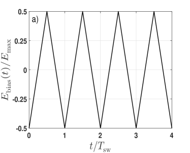
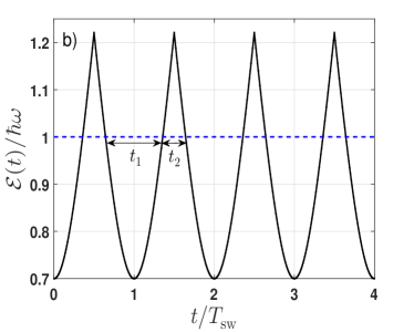
Figure 1: a) A triangular wave bias field $E_{\mathrm{bias}}(t)$ and b) the corresponding energy splitting $\mathcal{E}(t)=\sqrt{\Delta^{2}(t)+\Delta^{2}_{0}}$ of a TLS with bias energy $\Delta(t)=0.5+2pE_{\mathrm{bias}}(t)$, tunneling energy $\Delta_{0}=0.7$, and $pE_{\mathrm{max}}=0.5$ (energies are in units of $\hbar\omega$). The intersections of $\mathcal{E}(t)$ with the dashed line correspond to times where the TLS is swept through resonance with the resonator, the dynamics of each resonance is of the LZ type, with the Hamiltonian (3). In each period of the bias field, the time intervals $t_{1}$ and $t_{2}$ correspond to free propagation between subsequent LZ transitions, with $t_{1}+t_{2}=T_{\mathrm{sw}}$.

To obtain the dielectric loss due to TLSs, we calculate the counting statistics of the number of photons absorbed by a single TLS. Within the full counting statistics formalism, the evolution operator describing a single coherent LZ transition is SSN10

$$\mathcal{U}_{\mathrm{LZ}}(k)=\begin{pmatrix}\sqrt{P}&e^{i\frac{k}{2}}e^{-i\psi}\sqrt{1-P}\\ -e^{-i\frac{k}{2}}e^{i\psi}\sqrt{1-P}&\sqrt{P}\end{pmatrix},$$ (4)

where $\psi$ is the Stokes phase, approaching 0 and $\pi/4$ in the adiabatic ($\xi\ll 1$) and non-adiabatic ($\xi\gg 1$) limits, respectively SE91 . Note that a sign reversal of $v$ in the Hamiltonian (3) corresponds to the transformation $\psi\rightarrow\pi-\psi$ in Eq. (4) SSN10 ; Supp . The counting field $k$ counts the number of photons absorbed by the TLS, with the factors $e^{-ik/2}$ and $e^{ik/2}$ corresponding to the absorption and emission of a photon. In Liouville space Supp , this evolution operator transforms into the superoperator $U_{\mathrm{LZ}}(k)=\mathcal{U}_{\mathrm{LZ}}(k)\otimes\left[\mathcal{U}_{\mathrm{LZ}}(-k)\right]^{\ast}$.

In between two successive transitions, the TLS is out of resonance for a time interval $t$ and the dynamics of its density matrix $\rho$ is described by the Lindblad equation,

$$\dot{\rho}=-\frac{i}{\hbar}\left[\mathcal{H}_{\mathrm{TLS}},\rho\right]+\sum_{i=\pm}\Gamma_{i}\left(L_{i}\rho L^{{\dagger}}_{i}-\frac{1}{2}\{L^{{\dagger}}_{i}L_{i},\rho\}\right),$$ (5)

where $\mathcal{H}_{\mathrm{TLS}}(t)=(\mathcal{E}(t)/2)\sigma_{z}$, $L_{\pm}=\sigma_{\pm}=(\sigma_{x}\pm i\sigma_{y})/2$ and $\Gamma_{+}=\Gamma_{\uparrow}$, $\Gamma_{-}=\Gamma_{\downarrow}$ are the transition rates between the TLS eigenstates. For simplicity, we assume no pure dephasing, such that the decoherence rate is $\Gamma_{2}=\Gamma_{1}/2$, where $\Gamma_{1}=\Gamma_{\uparrow}+\Gamma_{\downarrow}$ is the relaxation rate. The corresponding evolution operator in Liouville space is Supp

$${\tiny U(t)=\begin{pmatrix}\frac{\Gamma_{\uparrow}}{\Gamma_{1}}+\frac{\Gamma_{\downarrow}}{\Gamma_{1}}e^{-\Gamma_{1}t}&0&0&\frac{\Gamma_{\uparrow}}{\Gamma_{1}}\left(1-e^{-\Gamma_{1}t}\right)\\ 0&e^{i\phi(t)-\Gamma_{2}t}&0&0\\ 0&0&e^{-i\phi(t)-\Gamma_{2}t}&0\\ \frac{\Gamma_{\downarrow}}{\Gamma_{1}}\left(1-e^{-\Gamma_{1}t}\right)&0&0&\frac{\Gamma_{\downarrow}}{\Gamma_{1}}+\frac{\Gamma_{\uparrow}}{\Gamma_{1}}e^{-\Gamma_{1}t}\end{pmatrix}},$$ (6)

where $\phi(t)=\frac{1}{\hbar}\int^{t}_{0}\mathcal{E}(t^{\prime})dt^{\prime}$. The evolution of the density matrix after one period of the bias field is obtained as $\ket{\rho(T_{\mathrm{sw}},k)}=U_{\mathrm{sw}}(k)\ket{\rho(0)}$, where $\ket{\rho}=(\rho_{00},\rho_{01},\rho_{10},\rho_{11})^{T}$ is the ket representing the density matrix $\rho$ in Liuoville space Supp , and $U_{\mathrm{sw}}(k)~{}=~{}U_{\mathrm{LZ}}(\pi-\psi,k)U(t_{2})U_{\mathrm{LZ}}(\psi,k)U(t_{1})$ with $T_{\mathrm{sw}}=t_{1}+t_{2}$ (here we have used the fact that the sweep rate changes sign between consecutive transitions). The evolution after time $t=NT_{\mathrm{sw}}$ is then

$$\ket{\rho(t,k)}=U^{N}_{\mathrm{sw}}(k)\ket{\rho(0)}.$$ (7)

The generating function for the statistics of the TLS photon absorption after time $t=NT_{\mathrm{sw}}$ is given by

$$\chi(t,k) =\mathrm{Tr}\left[\ket{\rho(t,k)}\right]=\mathrm{Tr}\left[U^{N}_{\mathrm{sw}}(k)\ket{\rho(0)}\right],$$ (8)

where the trace operation is defined as $\mathrm{Tr}\left[\ket{\rho}\right]\equiv\rho_{00}+\rho_{11}$. In particular, the number of photons absorbed by the TLS during time $t$ is given by the first moment $\braket{N_{\mathrm{ph}}(t)}=-i\frac{\partial\chi(t,k)}{\partial k}\big{|}_{k=0}$. For $k=0$ there should be a stationary solution to Eq. (7), meaning that one of the eigenvalues $\lambda_{1}$ of $U_{\mathrm{sw}}(k=0)$ equals unity, whereas $|\lambda_{j}|<1$ for $j=2,3,4$. As a result, in the limit $t\rightarrow\infty$ only the mode with eigenvalue $\lambda_{1}=1$ will contribute, and after some algebra we obtain the photon absorption rate per TLS Supp ,

$$\gamma_{\mathrm{abs}}=\lim_{t\rightarrow\infty}\frac{\braket{N_{\mathrm{ph}}(t)}}{t}=-\frac{i}{T_{\mathrm{sw}}}\bra{g_{1}}\frac{dU_{\mathrm{sw}}}{dk}\bigg{|}_{k=0}\ket{v_{1}},$$ (9)

where $\bra{g_{1}}$ and $\ket{v_{1}}$ are the left and right eigenvectors of $U_{\mathrm{sw}}(k=0)$ corresponding to the eigenvalue $\lambda_{1}=1$. The total photon absorption rate per unit volume is $\Gamma_{\mathrm{abs}}=n_{\mathrm{TLS}}\gamma_{\mathrm{abs}}\propto P_{0}\,pE_{\mathrm{max}}\gamma_{\mathrm{abs}}$. Comparing the power dissipation density $P_{\mathrm{dis}}=-\hbar\omega\Gamma_{\mathrm{abs}}$ with $P_{\mathrm{dis}}=-\frac{1}{2}\omega\epsilon^{\prime\prime}E^{2}_{\mathrm{ac}}$, we obtain the expression for the loss tangent

$$\tan\delta=\frac{\epsilon^{\prime\prime}}{\epsilon^{\prime}}=\frac{2\hbar\Gamma_{\mathrm{abs}}}{\epsilon E^{2}_{\mathrm{ac}}}=\frac{2p^{2}\Gamma_{\mathrm{abs}}}{\epsilon\hbar\Omega^{2}_{\mathrm{R}0}},$$ (10)

where $\epsilon^{\prime}$ and $\epsilon^{\prime\prime}$ are the real and imaginary parts of the dielectric constant.

The general expression for $\gamma_{\mathrm{abs}}$ is somewhat complicated, see Eq. (26) in the supplementary material Supp . We now consider the experimentally relevant regime $k_{\mathrm{B}}T\ll\hbar\omega$, for which $\Gamma_{1}\approx\Gamma_{\downarrow}$ ($\Gamma_{\uparrow}\approx 0$), and analyze the expression for $\gamma_{\mathrm{abs}}$ in simple limits. We first consider the incoherent limit $\Gamma_{1}T_{\mathrm{sw}}\gg 1$, which in terms of the dimensionless sweep rate $\xi$ can be expressed as $\xi\ll\xi_{2}$, with $\xi_{2}\equiv 8pE_{\mathrm{max}}\Gamma_{1}/(\pi\hbar\Omega^{2}_{\mathrm{R}0})$. In this limit we obtain $\gamma_{\mathrm{abs}}\approx 2\left(1-P\right)/T_{\mathrm{sw}}$. Equation (10) then gives the universal behavior discussed in Refs. BAL13 ; KMS14 , namely $\tan\delta/\tan\delta_{0}\approx 1$ in the non-adiabatic limit $\xi\gg 1$, and $\tan\delta/\tan\delta_{0}\approx\xi$ for $\xi_{1}\ll\xi\ll 1$ Supp . Thus, the results of Refs. BAL13 ; KMS14 are reproduced if subsequent LZ transitions are incoherent such that TLSs start from the ground state at each transition. We note that the regime $\xi<\xi_{1}=2\Gamma_{1}/(\pi\Omega_{\mathrm{R}0})$, in which dissipation occurs within a single LZ transition, has to be treated separately. In this limit the loss approaches the saturation limit $\tan\delta/\tan\delta_{0}=1/\sqrt{1+(\Omega_{\mathrm{R}0}/\Gamma_{1})^{2}}$, as studied numerically in Ref. BAL13 . As mentioned above, in this work we concentrate on the regime $\xi>\xi_{1}$, where dissipation within a single transition can be safely neglected, and consider the effect of dissipation between transitions.

In the coherent regime $\Gamma_{1}T_{\mathrm{sw}}\ll 1$ or $\xi\gg\xi_{2}$, TLSs experience $M=\left(\Gamma_{1}T_{\mathrm{sw}}\right)^{-1}=\xi/\xi_{2}\gg 1$ multiple coherent transitions. In the non-adiabatic regime $\xi\gg 1$, where the probability $1-P$ for photon absorption\emission in a single transition is small, the interference between multiple transitions is constructive for $\phi_{1}+\phi_{2}=2\pi n$ Supp , where $n$ is an integer and $\phi_{1,2}$ are the dynamical phases accumulated between successive transitions. This gives rise to a resonance in $\gamma_{\mathrm{abs}}$ as a function of the phases, whose width in the non-adiabatic regime $\xi\gg 1$ is $\delta\phi\propto M^{-1}$ for $M^{2}\left(1-P\right)<1$ and $\delta\phi\propto\sqrt{1-P}$ for $M^{2}\left(1-P\right)>1$ Supp . The contribution to $\gamma_{\mathrm{abs}}$ of TLSs out of resonance (corresponding to destructive interference Supp ) is $\gamma^{\mathrm{non-res}}_{\mathrm{abs}}\propto\Gamma_{1}\left(1-P\right)=\Gamma_{1}/\xi$, with weak dependence on $\phi_{1}$ and $\phi_{2}$. Below we concentrate on the contribution of the resonance, which dominates over that of the off-resonance part.

To obtain the loss tangent due to an ensemble of TLSs, one has to compute the total absorption rate per unit volume [see Eq. (10)], $\Gamma_{\mathrm{abs}}$, by averaging $\gamma_{\mathrm{abs}}$ over the distribution of TLSs and the orientation of their dipole moments, as described in the supplementary material Supp . This is a complicated procedure Supp , and instead we choose to concentrate on the main effect of the ensemble of TLSs relevant to the interference discussed above, which is the distribution of the phases $\phi_{1}$ and $\phi_{2}$. It is plausible to assume that the wide, random distribution of TLS parameters translates into an approximately homogeneous distribution of $\phi_{1}$ and $\phi_{2}$. We thus neglect the distribution of $\Delta_{0}$, $p$ and $\eta$ in all other quantities, such as the sweep rate, the Rabi frequency, the relaxation rate and the stokes phase, and set $t_{1}=t_{2}=T_{\mathrm{sw}}/2$ (the qualitative results are not sensitive to the latter choice). The absorption rate per TLS, $\gamma_{\mathrm{abs}}$, is then a function of $\xi$, $\xi_{2}$, $\phi_{1}$ and $\phi_{2}$ Supp . Two different behaviors of the loss tangent in the coherent regime are expected for $\xi_{2}<1$ and $\xi_{2}>1$.

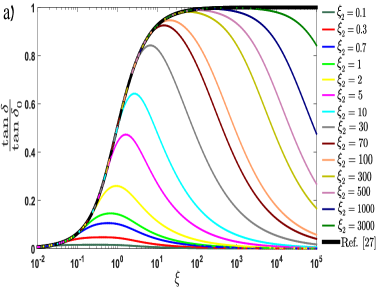
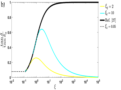
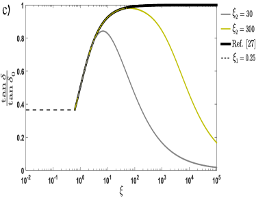
Figure 2: Theoretical results for the loss tangent due to TLSs, normalized by the intrinsic low-power loss tangent $\tan\delta_{0}=\pi P_{0}p^{2}/(3\epsilon)$, as a function of the dimensionless sweep rate $\xi\equiv 2|v_{0}|/(\pi\hbar\Omega^{2}_{\mathrm{R}0})$ for various values of $\xi_{2}\equiv 8pE_{\mathrm{max}}\Gamma_{1}/(\pi\hbar\Omega^{2}_{\mathrm{R}0})$, as indicated in the legend. The results are obtained by a numerical average of the photon absorption rate per TLS, $\braket{\gamma_{\mathrm{abs}}}$, over a homogeneous distribution of the phases $\phi_{1}$ and $\phi_{2}$. a) Calculation in the limit $\xi_{1}=2\Gamma_{1}/(\pi\Omega_{\mathrm{R}0})\rightarrow 0$ and $pE_{\mathrm{max}}/(\hbar\Gamma_{1})\rightarrow\infty$ such that $\xi_{2}=8pE_{\mathrm{max}}\Gamma_{1}/(\pi\hbar\Omega^{2}_{\mathrm{R}0})=2\pi\xi^{2}_{1}pE_{\mathrm{max}}/(\hbar\Gamma_{1})$ is finite, corresponding to full saturation at zero sweep rate. b) Modification of the results for the case of partial saturation at zero sweep rate (finite $\xi_{1}$), with $\xi_{1}=0.05$ and c) $\xi_{1}=0.25$. The loss in a) is cut by the saturation value $\tan\delta/\tan\delta_{0}=1/\sqrt{1+(\Omega_{\mathrm{R}0}/\Gamma_{1})^{2}}$ (horizontal dashed line), to which it approaches for $\xi\lesssim\xi_{1}$ BAL13 ; KMS14 . Due to the decoupling effect at high sweep rates the loss reduces below its value in the absence of a periodic bias field ($\xi=0$).

For $\xi_{2}<1$, the regime $\xi_{2}<\xi\ll 1$ is coherent ($\xi>\xi_{2}$) and adiabatic ($\xi\ll 1$), meaning that photons are absorbed and re-emitted by the TLSs with high probability. The photons are thus dissipated at the relaxation rate of the TLSs, so that $\gamma_{\mathrm{abs}}\propto\Gamma_{1}$ Supp . This gives rise to constant loss tangent, $\tan\delta\propto\xi_{2}$. In the non-adiabatic regime $\xi_{2}<1\ll\xi$ the resonance width is $\delta\phi\propto\sqrt{1-P}$ (since $M^{2}\left(1-P\right)\approx\xi/\xi^{2}_{2}\gg 1$ in this regime). If $\phi_{1}$ and $\phi_{2}$ are nearly homogeneously distributed, the contribution of this resonance to the photon absorption rate is $\gamma^{\mathrm{res}}_{\mathrm{abs}}\propto\gamma_{\mathrm{abs}}(\phi_{1}=-\phi_{2})\cdot\delta\phi\propto\Gamma_{1}\sqrt{1-P}$. Hence, the loss tangent decreases as $\xi^{-1/2}$.

For $\xi_{2}>1$, the loss tangent follows the universal curve of Ref. BAL13 up to $\xi\sim\xi_{2}$. For $\xi\gg\xi^{2}_{2}$ the resonance width is again $\delta\phi\propto\sqrt{1-P}$, and the corresponding contribution of this resonance to the loss tangent is again $\propto\xi^{-1/2}$. In the crossover region $\xi_{2}<\xi\ll\xi^{2}_{2}$ the resonance width is $\delta\phi\propto M^{-1}$, giving rise to the photon absorption rate $\gamma^{\mathrm{res}}_{\mathrm{abs}}\approx\gamma_{\mathrm{abs}}(\phi_{1}=-\phi_{2})\cdot\delta\phi\propto\Gamma_{1}M\left(1-P\right)$, which depends weakly on $\xi$. Table 1 summarizes the qualitative behavior of the loss tangent in various regimes.

	$\xi_{2}<1$			$\xi_{2}>1$
	$\xi<\xi_{2}$	$\xi_{2}<\xi\ll 1$	$\xi\gg 1$	$\xi\ll 1$	$1\ll\xi<\xi_{2}$	$\xi_{2}<\xi\ll\xi^{2}_{2}$	$\xi\gg\xi^{2}_{2}$
$\tan\delta/\tan\delta_{0}$	$\propto\xi$	$\propto\xi_{2}$	$\propto\xi_{2}/\sqrt{\xi}$	$\propto\xi$	$\propto 1$	$\propto 1$	$\propto\xi_{2}/\sqrt{\xi}$

Table 1: Qualitative behavior of the normalized loss tangent $\tan\delta/\tan\delta_{0}$ in various regimes.

In Fig. 2a) we show the results for the loss tangent obtained by a numerical average of the absorption rate over the homogeneous distribution of $\phi_{1}$ and $\phi_{2}$. One readily observes the qualitative limits discussed above. The results in Fig. 2a) are obtained for the limit $\xi_{1}=2\Gamma_{1}/(\pi\Omega_{\mathrm{R}0})\rightarrow 0$, such that TLSs are fully saturated at zero sweep rate (i.e., we take the limits $\xi_{1}\rightarrow 0$ and $pE_{\mathrm{max}}/(\hbar\Gamma_{1})\rightarrow\infty$ such that $\xi_{2}=8pE_{\mathrm{max}}\Gamma_{1}/(\pi\hbar\Omega^{2}_{\mathrm{R}0})=2\pi\xi^{2}_{1}pE_{\mathrm{max}}/(\hbar\Gamma_{1})$ is finite). This shows how the universal curve discussed in Ref. BAL13 (solid black curve in Fig. 2a)) is modified due to multiple coherent transitions. Note that under this assumption the loss at high sweep rates cannot reduce below the vanishing loss at $\xi=0$.

In order to relate directly to experiment, we note that for finite $\xi_{1}$ the loss approaches the saturation limit $\tan\delta/\tan\delta_{0}=1/\sqrt{1+(\Omega_{\mathrm{R}0}/\Gamma_{1})^{2}}=1/\sqrt{1+(2/\pi\xi_{1})^{2}}$ for $\xi<\xi_{1}$ BAL13 ; KMS14 . In Figs. 2b) and  2c) we show the theoretical results expected for finite values of $\xi_{1}$. For each value of $\xi_{2}>\xi_{1}$ (which translates to a given value of $pE_{\mathrm{max}}/(\hbar\Gamma_{1})=\xi_{2}/(2\pi\xi^{2}_{1})$), the results in Fig. 2a) describe the loss at $\xi>\xi_{1}$. For $\xi<\xi_{1}$ we cut these results by the horizontal lines corresponding to the value of the loss at the stationary saturation limit $\xi=0$. In practice, for $\xi\lesssim\xi_{1}$ the loss tangent reduces to its $\xi=0$ value monotonically with decreasing $\xi$, as was studied numerically in Refs. BAL13 ; KMS14 . Thus, in the regime $\xi_{1}<\xi<\xi_{2}$ the loss tangent is described by the universal curve discussed in Ref. BAL13 , whereas it becomes non-universal for $\xi<\xi_{1}$ (due to dissipation within a single transition) or $\xi>\xi_{2}$ (due to coherent multiple transitions). As seen in Figs. 2b) and  2c), for finite $\xi_{1}$ one expects the loss at high sweep rates ($\xi\gg\xi_{2}$) to decrease below its value at $\xi=0$. All the main qualitative features of our theoretical results are observed experimentally. This includes also the saturation of the loss at $\xi<\xi_{1}$, and to some extent the decrease below this value at large sweep rates (see Fig. 4 below).

We stress that the decrease of the loss at the coherent and non-adiabatic regime $\xi\gg\max\{1,\xi_{2}\}$ is a result of interference between $M$ coherent LZ transitions, which reduce the photon absorption probability. To see this, consider $N$ identical TLSs of which $N_{\mathrm{g}}(t)$ and $N_{\mathrm{e}}(t)$ occupying the ground and excited states, respectively. In a classical approach Comment1 , one can write a rate equation for $N_{\mathrm{e}}(t)$,

$$\dot{N}_{\mathrm{e}} =\gamma(N_{\mathrm{g}}-N_{\mathrm{e}})-\Gamma_{\downarrow}N_{\mathrm{e}}+\Gamma_{\uparrow}N_{\mathrm{g}}$$

$$=\gamma(N-2N_{\mathrm{e}})-\Gamma_{1}N_{\mathrm{e}}+\Gamma_{\uparrow}N,$$ (11)

where $\gamma=2\left(1-P\right)/T_{\mathrm{sw}}$ is the photon emission and absorption rate in a single LZ transition. The steady state solution is $N_{\mathrm{e}}=N(\gamma+\Gamma_{\uparrow})/\left(2\gamma+\Gamma_{1}\right)$ and the corresponding photon absorption rate per TLS is

$$\gamma_{\mathrm{abs}}=\frac{\gamma\left(N-2N_{\mathrm{e}}\right)}{N}=\frac{\Gamma_{\downarrow}-\Gamma_{\uparrow}}{\Gamma_{1}}\frac{\gamma}{1+2\gamma/\Gamma_{1}}.$$ (12)

Since $(\Gamma_{\downarrow}-\Gamma_{\uparrow})/\Gamma_{1}=\tanh(\hbar\omega/2k_{\mathrm{B}}T)$ equals unity at low temperatures, we obtain $\gamma_{\mathrm{abs}}\approx\gamma$ for $\gamma\ll\Gamma_{1}$ (or $M(1-P)\ll 1$) and $\gamma_{\mathrm{abs}}\approx\Gamma_{1}/2$ for $\gamma\gg\Gamma_{1}$ (or $M(1-P)\gg 1$). The first limit corresponds to the result of Refs. KMS14 ; BAL13 and the second limit corresponds to a constant loss tangent $\tan\delta\propto\xi_{2}$, as we find above in the regime $\xi_{2}<\xi\ll 1$. Therefore, a classical approach based on independent transitions does not capture the physics of the fast sweep regime, which exhibits a decreasing loss with increasing sweep rate for $\xi>\xi_{2}$.

II.2 Experiment

In our experiment, we study TLS in deposited aluminum oxide by using it as the dielectric in lumped-element LC-resonators. This material is highly relevant for superconducting quantum processors, because it is used for tunnel barriers in Josephson junctions of qubits and also forms naturally on circuit wiring after air exposure. However, any depositable dielectric can in principle be studied with this method.

Figure 3 shows a sample resonator structured by optical lithography from superconducting aluminum on a sapphire substrate. Following experiments by Khalil et al. KMS14 , the capacitances are designed as bridges consisting of four equal Al/AlOx/Al capacitors. Hereby, an electric bias field can be applied to the dielectric. In addition, our setup allows for mechanical TLS tuning by controlling the strain in the sample material with a piezo actuator LJ15 . Each chip contains 8 slightly different resonators that are coupled to a common transmission line, and is installed in a well-shielded and heavily filtered cryogenic setup that allows for measurements in the single-photon regime at sample temperatures of 30 mK BJD17 . All capacitors contain a 25-nm thick layer of amorphous AlO_x that is deposited in a Plassys system by eBeam-evaporation of aluminum in a low-pressure oxygen atmosphere. Further details on the setup and fabrication are found in Supp .

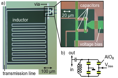
Figure 3: a) Photograph of a lumped-element resonator consisting of a capacitively terminated meandering inductor. The (colorized) inset shows a zoom of the four capacitors between bottom (red) and top layers (green), which are separated by 25nm-thick amorphous AlO_x. b) Circuit schematic. The electric field in the capacitor dielectric is controlled by an applied bias voltage $V_{\mathrm{bias}}$.

We characterize the total dielectric loss tangent $\tan\delta\equiv 1/Q_{i}$ by recording resonance curves using a network analyzer and extracting the internal quality factor $Q_{i}$ using a standard fit procedure PS15 . In particular, we study this loss while a triangular voltage signal $V_{\mathrm{bias}}(t)$ is applied as a bias to the sample dielectric. This results in a sweep rate $v_{0}=p\dot{V}_{\mathrm{bias}}/d$, where $d=25\,$nm is the distance between the capacitor plates, considering that due to the design only half the voltage drops at each capacitor. The shortest periods in our experiment are $10\,$ns, such that $T_{\mathrm{sw}}\gg 2\pi/\omega$, where $\omega\approx 2\pi\times 7\,$GHz is the resonance frequency of the resonator. Resonant transitions due to the bias field can therefore be safely neglected. The highest bias field amplitude is $E_{\mathrm{max}}=0.9\,$MV/m, which allows us to apply a bias field rate $\dot{E}_{\mathrm{bias}}=2E_{\mathrm{max}}/T_{\mathrm{sw}}$ up to $1.8\cdot 10^{14}\,\mathrm{V}/(\mathrm{m}\cdot\mathrm{s})$. For typical values of the dipole moment of TLSs in AlO_x, $p\approx 0.5\,e\AA$, this corresponds to a maximum sweep rate of $|v_{0}|/h\approx 2\cdot 10^{9}\,$GHz/s. The adiabatic condition $v_{0}/(\hbar\omega^{2})\ll 1$ thus holds, justifying the assumption that the bias field changes the energy splitting of the TLS adiabatically. We also note that as in Refs. BJD17 ; SB15 ; SB16 , the dielectric volume of the resonator has been chosen such that on average there is roughly one TLS in resonance with the resonator in the absence of the bias field. By applying the bias field all TLSs within the energy window $pE_{\mathrm{max}}$ around $\hbar\omega$ are swept into resonance and contribute to the loss. In our experiment $pE_{\mathrm{max}}$ is in the range $1-10\,$GHz, hence $\sim 100-1000$ TLSs contribute to the loss and averaging is proper.

Figure 4 shows the measured dielectric loss tangent in two different resonators as a function of the dimensionless sweep rate $\xi=2|v_{0}|/(\pi\hbar\Omega^{2}_{\mathrm{R}0})$. Each curve is obtained by varying the period $T_{\mathrm{sw}}$ of the bias field, keeping its amplitude $E_{\mathrm{max}}$ and the input power $P_{\mathrm{in}}$ fixed. To calculate $\xi$, the maximum Rabi frequency is computed as $\Omega_{\mathrm{R}0}=pE_{\mathrm{ac}}/\hbar=\sqrt{\left(p^{2}P_{\mathrm{in}}Q^{2}_{l}\right)/\left(\hbar^{2}\omega CQ_{\mathrm{c}}d^{2}\right)}$, where $Q_{l}$, $Q_{c}$ are the measured loaded and coupling quality factors, $C$ is the total resonator capacitance, and a typical value of $p=0.5\,$e$\AA$ is used MC18 . Note that for a given $P_{\mathrm{in}}$, the value of $E_{\mathrm{ac}}$ (and thus $\Omega_{\mathrm{R0}}$) depends on the resonator loss (and thus on $\xi$). The values of $\xi$ in the horizontal axes of Fig.  4 take this dependence into account.

To compare the experimental results with our theory, Fig. 4 shows the loss due to TLSs, obtained by subtracting the background loss at the saturation regime (large powers) at $\xi=0$. We further normalize the resulting loss tangent by the intrinsic loss tangent $\tan\delta_{0}$ (see Supp for saturation curves of the resonators and for values of the background and intrinsic TLS loss tangent). In addition, we estimate the values of the parameter $\xi_{2}=8pE_{\mathrm{max}}\Gamma_{1}/(\pi\hbar\Omega^{2}_{\mathrm{R}0})$ for selected curves. For this purpose, we use the value of $\Omega_{\mathrm{R0}}$ at $\xi=0$ and set $p=0.5\,e\AA$ and $\Gamma_{1}=1\,$MHz, in accordance with TLS dipole moments and relaxation rates observed in AlO_x MC18 ; SY10 ; LJ10 ; LJ16 . Note that this is an approximation, since the value of $\xi_{2}$ is not constant for measurement at a fixed power (due to the loss dependence of the Rabi frequency discussed above). For both resonators, the qualitative agreement with the theoretical prediction of Figs. 2 is excellent. By tuning the input power, and therefore varying $\Omega_{\mathrm{R0}}$, one can change the parameter $\xi_{2}$ by several orders of magnitude to obtain the different behaviors shown in Figs. 2. Variation of $E_{\mathrm{max}}$ then weakly tunes the value of $\xi_{2}$ in each regime. For $\xi_{2}\lesssim 1$ one observes wide peaks which become more pronounced for $1\lesssim\xi_{2}<100$. For $\xi_{2}>100$ these peaks become the universal plateau as in Fig. 4b), followed by the reduction in loss. Note that for $\xi_{2}>1$ the loss starts decreasing at $\xi\approx\xi_{2}$, in agreement with the theoretical prediction of Fig. 2a). Unfortunately, comparison of the functional form of this decrease with the power low $\tan\delta\propto\xi^{-1/2}$ predicted by our theory is impossible, both because there is almost no data at the regime $\xi>\xi^{2}_{2}$ and because of the dependence of $\Omega_{\mathrm{R}0}$ on $\xi$, not taken into account by the theory. We also notice that resonator 1 [Fig. 4a)] provides some evidence that the loss at high sweep rates can reduce below its value at $\xi=0$ (no bias field). This is seen for the green and blue curve families for which the TLSs are not fully saturated at $\xi=0$.

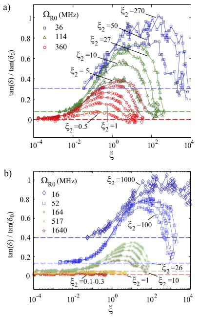
Figure 4: Normalized dielectric loss as a function of the dimensionless sweep rate $\xi$ for various values of $\xi_{2}$ which were set by the applied microwave power (coloured curve families) and the amplitude of the bias field (varied in the range $89.5-806$ kV/m) a) for resonator 1 and b) resonator 2. For each family of curves obtained with the same input power, the legend shows the corresponding value of $\Omega_{\mathrm{R}0}$ calculated at $\xi=0$. Horizontal dashed lines indicate the resonator loss when it is driven at the power levels of the curve families without applied bias field. Negative loss values are within the standard deviation.

III The single-photon regime and correspondence to a qubit coupled to resonant TLSs

To examine whether the effect discussed above is also applicable in the single-photon regime, we consider now a quantized single-mode cavity field $\mathbf{E}_{\mathrm{res}}(t)=\hat{\mathbf{e}}\sqrt{\hbar\omega/\epsilon_{0}V}(ae^{-i\omega t}+a^{{\dagger}}e^{i\omega t})\sin(kz)$ ($\hat{\mathbf{e}}$ is a polarization unit vector, $\epsilon_{0}$ the vacuum permittivity, $V$ the resonator volume, $k$ the wave vector, and $a^{{\dagger}}$, $a$ the photon creation and annihilation operators) propagating along the $z$-axis and interacting with a set of near-resonant TLSs. After neglecting the longitudinal coupling and applying the rotating wave approximation, the corresponding Hamiltonian is

$$\mathcal{H}= \frac{1}{2}\sum_{i}\mathcal{E}_{i}\sigma^{i}_{z}+\hbar\omega a^{{\dagger}}a+\sum_{i}g_{i}\left(\sigma^{i}_{+}a+\sigma^{i}_{-}a^{{\dagger}}\right),$$ (13)

where $g_{i}=-p(\Delta_{0}/\mathcal{E}_{i})\sqrt{\hbar\omega/\epsilon_{0}V}\sin(kz_{i})$ and $\sigma_{\pm}=(\sigma_{x}\pm i\sigma_{y})/2$. As the last term couples different TLSs via the quantized cavity field, the assumption of independent TLSs cannot be invoked as in the case of a classical field discussed above (which corresponds to the substitution $2g_{i}\sqrt{n_{\mathrm{ph}}}=\Omega_{\mathrm{R},i}$). For $\braket{n_{\mathrm{ph}}}\gg 1$, each TLS feels the same classical field in every transition, but for $\braket{n_{\mathrm{ph}}}\sim 1$ the dynamics of each transition depends on previous transitions of other TLSs. In this regime, calculation of the probability for an absorption of a single photon involves a consideration of multiple emissions and absorptions by an ensemble of TLSs, and thus the interference between many more paths than in the above analysis, where the coherent evolution of a single TLS was considered. It is expected, however, that just as in the case of independent TLSs discussed above, the random distribution of TLSs leads to random distribution of phases accumulated between consecutive transitions. As a result, there will be no preference for some resonant paths that involve emissions and absorptions of multiple TLSs, and most paths will interfere destructively, thus justifying an independent treatment of each TLS. In this case, each TLS is described by a Jaynes-Cummings Hamiltonian BM11 ,

$$\mathcal{H}=\frac{1}{2}\mathcal{E}\sigma_{z}+\hbar\omega a^{{\dagger}}a+g\left(\sigma_{+}a+\sigma_{-}a^{{\dagger}}\right),$$ (14)

which reduces to the LZ Hamiltonian in the vicinity of each resonance. Provided this approximation is justified, the physics discussed above is also applicable in the single-photon regime. Indeed, in Fig. 4 the data at the lowest Rabi frequency corresponds to mean photon number $\braket{n_{\mathrm{ph}}}\approx 1$, and clearly displays reduced loss at high sweep rates, suggesting that a treatment of independent TLSs is indeed relevant. A more thorough investigation of the single-photon regime will be performed elsewhere.

We note that the single-photon regime $\braket{n_{\mathrm{ph}}}\ll 1$ corresponds to the problem of a qubit with energy splitting $\mathcal{E}_{\mathrm{q}}$ coupled to a near-resonant TLS with energy splitting $\mathcal{E}_{\mathrm{TLS}}$ Comment3 . Near resonance the relevant coupling is the transverse one, $\propto\sigma^{(\mathrm{q})}_{x}\sigma^{(\mathrm{TLS})}_{x}$, and within the subspace $\{\ket{0,e},\ket{1,g}\}$ ($\ket{0},\ket{1}$ and $\ket{g},\ket{e}$ being the qubit and the TLS ground and excited states, respectively) each resonance is again governed by the LZ dynamics. The above results thus suggest that by sweeping the bias energy of TLSs at a rate larger than their relaxation rate, but smaller than the qubit frequency $\omega_{\mathrm{q}}=\mathcal{E}_{\mathrm{q}}/\hbar$, one may dynamically decouple the qubit from sparse TLSs. Since this sweeping is slow compared to the time scale of the qubit dynamics, the qubit state remains unperturbed. This is in contrast to the saturation regime at strong resonant driving fields, where undesired qubit excitations are inevitable.

Data Availability

Data sets generated and analyzed during the current study are available from the corresponding author on request.

Author Contributions

S.M. developed the theoretical model and performed the calculations in collaboration with A.S. and M.S.; The samples were fabricated by H.S. and A.B.; Measurements were done by H.S. and J.L.; S.M. and J.L. wrote the paper with contributions from all authors.

Additional Information

Supplementary information accompanies this paper.
Competing interests: The authors declare that there are no competing interests.

References

- (1) G. Wendin, Rep. Prog. Phys. 80, 106001 (2017).
- (2) C. Neill, P. Roushan, K. Kechedzhi, S. Boixo, S. V. Isakov, V. Smelyanskiy, R. Barends, B. Burkett, Y. Chen, Z. Chen, B. Chiaro, A. Dunsworth, A. Fowler, B. Foxen, R. Graff, E. Jeffrey, J. Kelly, E. Lucero, A. Megrant, J. Mutus, M. Neeley, C. Quintana, D. Sank, A. Vainsencher, J. Wenner, T. C. White, H. Neven, and J. M. Martinis, Science 360, 195 (2018).
- (3) J. S. Otterbach, R. Manenti, N. Alidoust, A. Bestwick, M. Block, B. Bloom, S. Caldwell, N. Didier, E. Schuyler Fried, S. Hong, P. Karalekas, C. B. Osborn, A. Papageorge, E. C. Peterson, G. Prawiroatmodjo, N. Rubin, C. A. Ryan, D. Scarabelli, M. Scheer, E. A. Sete, P. Sivarajah, R. S. Smith, A. Staley, N. Tezak, W. J. Zeng, A. Hudson, B. R. Johnson, M. Reagor, M. P. da Silva, and C. Rigetti, arXiv:1712.05771 (2017).
- (4) P. Day, H.G. LeDuc, B. A. Mazin, A. Vayonakis, and J. Zmuidzinas, Nature (London) 425, 817 (2003).
- (5) J. Zmuidzinas, Annu. Rev. Condens. Matter Phys. 3, 169 (2012).
- (6) A. Wallraff, D. I. Schuster, A. Blais, L. Frunzio, R.-S. Huang, J. Majer, S. Kumar, S. M. Girvin, and R. J. Schoelkopf, Nature (London) 431, 162 (2004).
- (7) J. Q. You and F. Nori, Nature (London) 474, 589 (2011).
- (8) X. Gu, A. F. Kockum, A. Miranowicz, Y.-X. Liu, and F. Nori, Phys. Rep. 718-719, 1 (2017).
- (9) W. A. Phillips, J. Low-Temp. Phys. 7, 351 (1972).
- (10) P. W. Anderson, B. I. Halperin, and C. M. Varma, Philos. Mag. 25, 1 (1972).
- (11) C. Müller, J. H. Cole, and J. Lisenfeld, arXiv:1705.01108 (2017).
- (12) Y. J. Rosen, M. A. Horsley, S. E. Harrison, E. T. Holland, A. S. Chang, T. Bond, and J. L. DuBois, Appl. Phys. Lett. 114, 202601 (2019).
- (13) A. Bilmes, S. Zanker, A. Heimes, M. Marthaler, G. Schön, G. Weiss, A. V. Ustinov, and J. Lisenfeld, Phys. Rev. B 96, 064504 (2017).
- (14) J. Lisenfeld, G. J. Grabovskij, C. Müller, J. H. Cole, G. Weiss, and A. V. Ustinov, Nature Comm. 6, 6182 (2015).
- (15) C. Müller, J. Lisenfeld, A. Shnirman, and S. Poletto, Phys. Rev. B 92, 035442 (2015).
- (16) S. Meißner, A. Seiler, J. Lisenfeld, A. V. Ustinov, and G. Weiss, Phys. Rev. B 97, 180505 (2018).
- (17) P. V. Klimov, J. Kelly, Z. Chen, M. Neeley, A. Megrant, B. Burkett, R. Barends, K. Arya, B. Chiaro, Y. Chen, A. Dunsworth, A. Fowler, B. Foxen, C. Gidney, M. Giustina, R. Graff, T. Huang, E. Jeffrey, E. Lucero, J. Y. Mutus, O. Naaman, C. Neill, C. Quintana, P. Roushan, D. Sank, A. Vainsencher, J. Wenner, T. C. White, S. Boixo, R. Babbush, V. N. Smelyanskiy, H. Neven, and J. M. Martinis, Phys. Rev. Lett. 121, 090502 (2018).
- (18) C. Neill, A. Megrant, R. Barends, Y. Chen, B. Chiaro, J. Kelly, J. Y. Mutus, P. J. J. O’Malley, D. Sank, J.Wenner, T. C. White, Y. Yin, A. N. Cleland, and J. M. Martinis, Appl. Phys. Lett. 103, 072601 (2013).
- (19) J. Burnett, L. Faoro, I. Wisby, V. L. Gurtovoi, A. V. Chernykh, G. M. Mikhailov, V. A. Tulin, R. Shaikhaidarov, V. Antonov, P. J. Meeson, A. Y. Tzalenchuk, and T. Lindström, Nat. Commun. 5, 4119 (2014).
- (20) L. Faoro, and L. B. Ioffe, Phys. Rev. B 91, 014201 (2015).
- (21) A. L. Burin, S. Matityahu, and M. Schechter, Phys. Rev. B 92, 174201 (2015).
- (22) S. Schlör, J. Lisenfeld, C. Müller, A. Schneider, D. P. Pappas, A. V. Ustinov, and M. Weides, arXiv:1901.05352.
- (23) J. Burnett, A. Bengtsson, M. Scigliuzzo, D. Niepce, M. Kudra, P. Delsing, and J. Bylander, npj Quantum Inf. 5, 54 (2019).
- (24) C. T. Earnest, J. H. Béjanin, T. G. McConkey, E. A. Peters, A. Korinek, H. Yuan, and M. Mariantoni, Supercond. Sci. Technol. 31, 125013 (2018).
- (25) M. Von Schickfus and S. Hunklinger, Phys. Lett. A 64, 144 (1977).
- (26) At the regime of low temperatures considered here, the hyperbolic tangent factor is approximately unity, meaning that the thermal excitation of resonant TLSs is negligible.
- (27) A. L. Burin, M. S. Khalil, and K. D. Osborn, Phys. Rev. Lett. 110, 157002 (2013).
- (28) M. S. Khalil, S. Gladchenko, M. J. A. Stoutimore, F. C. Wellstood, A. L. Burin, and K. D. Osborn, Phys. Rev. B 90, 100201(R) (2014).
- (29) L. D. Landau, Phys. Z. Sov. 2, 46 (1932).
- (30) C. Zener, Proc. R. Soc. Ser. A 137, 696 (1932).
- (31) E. C. G. Stückelberg, Helv. Phys. Acta 5, 369 (1932).
- (32) S. N. Shevchenko, S. Ashhab, and F. Nori, Phys. Rep. 492, 1 (2010).
- (33) W. D. Oliver, Y. Yu, J. C. Lee, K. K. Berggren, L. S. Levitov, and T. P. Orlando, Science 310, 1653 (2005).
- (34) W. D. Oliver and S. O. Valenzuela, Quantum Inf. Process. 8, 261 (2009).
- (35) M. Sillanpää, T. Lehtinen, A. Paila, Y. Makhlin, and P. Hakonen, Phys. Rev. Lett. 96, 187002 (2006).
- (36) C. M. Wilson, G. Johansson, T. Duty, F. Persson, M. Sandberg, and P. Delsing, Phys. Rev. B 81, 024520 (2010).
- (37) A. Izmalkov, S. H. W. van der Ploeg, S. N. Shevchenko, M. Grajcar, E. Il’ichev, U. Hübner, A. N. Omelyanchouk, and H.-G. Meyer, Phys. Rev. Lett. 101, 017003 (2008).
- (38) M. D. LaHaye, J. Suh, P. M. Echternach, K. C. Schwab, and M. L. Roukes, Nature 459, 960 (2009).
- (39) See Supplementary Material for further details of theory and experiments.
- (40) It is important to realize that the LZ transitions occur between photon number states that differ by one photon. This does not contradict the assumption of a classical resonator with mean photon number , such that the transition amplitudes are fixed for all TLSs and do not change between consecutive transitions, which allows us to treat TLSs independently.
- (41) E. Shimshoni and Y. Gefen, Ann. Phys. (N.Y.) 210, 16 (1991).
- (42) J. D. Brehm, A. Bilmes, G. Weiss, A. V. Ustinov, and J. Lisenfeld, Appl. Phys. Lett. 111, 112601 (2017).
- (43) S. Probst, F. B. Song, P. A. Bushev, A. V. Ustinov, and M. Weides, Rev. Sci. Instr. 86, 024706 (2015).
- (44) B. Sarabi , A. N. Ramanayaka, A. L. Burin, F. C. Wellstood, and K. D. Osborn, Appl. Phys. Lett. 106, 172601 (2015).
- (45) B. Sarabi , A. N. Ramanayaka, A. L. Burin, F. C. Wellstood, and K. D. Osborn, Phys. Rev. Lett. 116, 167002 (2016).
- (46) Y. Shalibo, Y. Rofe, D. Shwa, F. Zeides, M. Neeley, J. M. Martinis, and N. Katz, Phys. Rev. Lett. 105, 177001 (2010).
- (47) J. Lisenfeld, C. Müller, J. H. Cole, P. Bushev, A. Lukashenko, A. Shnirman, and A.V. Ustinov, Phys. Rev. Lett. 105, 230504 (2010).
- (48) J. Lisenfeld, A. Bilmes, S. Matityahu, S. Zanker, M. Marthaler, M. Schechter, G. Schön, A. Shnirman, G. Weiss, and A. V. Ustinov, Sci. Rep. 6, 23786 (2016).
- (49) M. Bhattacharya, K. D. Osborn, and A. Mizel, Phys. Rev. B 84, 104517 (2011).
- (50) Note that a resonator is usually in a coherent state and not in a Fock state, and therefore its state cannot exactly be described as a superposition of two states. However, for mean photon number , the most important number states in the coherent superposition are the zero and one photon states, which are in correspondence to the ground and excited states of a qubit.