Efficient Consensus-based Formation Control With Discrete-Time Broadcast Updates

Abstract

This paper presents a consensus-based formation control strategy for autonomous agents moving in the plane with continuous-time single integrator dynamics. In order to save wireless resources (bandwidth, energy, etc), the designed controller exploits the superposition property of the wireless channel. A communication system, which is based on the Wireless Multiple Access Channel (WMAC) model and can deal with the presence of a fading channel is designed. Agents access the channel with simultaneous broadcasts at synchronous update times. A continuous-time controller with discrete-time updates is proposed. A proof of convergence is given and simulations are shown, demonstrating the effectiveness of the suggested approach.

I Introduction

In the context of autonomous multi-agent systems, coordination issues are of obvious importance. Both the design of coordination rules to achieve a desired overall behaviour and the analysis of emergent behaviours for given local interaction rules have been widely studied during the last two decades, e.g. [1, 2].

One particular coordination problem for a multi-agent system is formation control. A group of agents moving in space are required to converge towards a specific formation around a point, to be agreed on. A distributed way for agents to achieve such a formation is by executing a suitable consensus protocol, e.g., see [3]. Consensus is a distributed technique, where agents have to agree on a variable of common interest by exchanging information according to a given communication topology.

Often, energy consumption represents a critical aspect in multi-agent scenarios (e.g., when agents are battery powered). Then, the use of orthogonal channel access methods for inter-agent communication, which is standard, is less than ideal. In orthogonal channel access methods, information exchange is agent-to-agent and avoids interference by time or frequency multiplexing. Instead, the simultaneous broadcast of information and the exploitation of the wireless channel’s superposition property may be advantageous, see [4, 5, 6]. A problem in the context is that channel transmission properties are unknown and time-varying. This was addressed in [7], where a consensus protocol was suggested that can handle unknown channel coefficients. The possible computational saving by using broadcast-based protocol for so-called max-consensus problems was quantified in [8].

In the remainder of this paper, a consensus-based formation control strategy is proposed. Agents move in space with a continuous time dynamics and can synchronously broadcast at discrete-time steps. The proposed communication protocol makes use of the interference of broadcast signals. The formation control strategy takes inspiration from the consensus protocol presented in [9], where continuous-time dynamics and discrete-time communication were brought together.

The paper is organized as follows. Section II summarizes notation. Section III defines the formation control problem. A model of the wireless channel is presented in Section IV-A, and the communication system able to harness the superposition property is designed in Section IV-B. Based on this, Section V presents the consensus-based control strategy. Convergence of the overall scheme is given in Section VI. A comparison with the standard approach to the problem is in Section VII. Simulation results are shown in Section VIII. Finally, Section IX provides concluding remarks.

II Notation

Throughout this paper, $\mathbb{N}_{0}$, respectively $\mathbb{N}$, denotes the set of nonnegative, respectively positive, integers. The sets of real numbers, nonnegative real numbers, and positive real numbers are, respectively, denoted $\mathbb{R}$, $\mathbb{R}_{\geq 0}$, and $\mathbb{R}_{>0}$. Given a set $\mathbb{S}$, its cardinality is denoted by $|\mathbb{S}|$.

Given a matrix $A$ of dimension $n\times m$, the entry in position $(i,j)$ is $[A]_{ij}$. Matrix $A$ is positive (nonnegative) if $[A]_{ij}>0$ ($[A]_{ij}\geq 0$), $\forall i=1\dots n,\ \forall j=1\dots m$. A nonnegative matrix $A$ of dimension $n\times n$ is called reducible if there exists a permutation matrix $Q$ such that $QAQ^{-1}$ is of block upper-triangular form, i.e. $A$ is reducible if and only if it can be brought into upper block-triangular form by identical row and column permutations. If matrix $A$ is not reducible, is called irreducible. A nonnegative square matrix $A$ of dimension $n$ is primitive if $\exists h\in\mathbb{N}$, such that $A^{h}$ is positive. Two nonnegative matrices $A$ and $B$ of the same dimension are of the same type, and we write $A\sim B$, if they have positive entries in the same positions. $\mathbb{I}_{n}$ denotes the n-dimensional identity matrix, $\mathbf{0}_{n\times m}$ is a matrix of zeros with $n$ rows and $m$ columns, and $\mathbf{1}_{n\times m}$ is a matrix of ones with $n$ rows and $m$ columns.

A graph $\mathcal{G}$ is a pair $(\mathcal{N},\mathcal{A})$, where $\mathcal{N}=\{1\dots n\}$ is the set of nodes and $\mathcal{A}\subseteq\mathcal{N}\times\mathcal{N}$ set of arcs. $(i,j)\in\mathcal{A}$ if and only if an arc goes from node $i\in\mathcal{N}$ to node $j\in\mathcal{N}$. Given a sequence of graphs constructed on the same set of nodes, i.e. $\{\mathcal{G}(k)\}_{k\in\mathbb{N}_{0}}$, the set

$$\mathcal{N}_{i}(k):=\{j\in\mathcal{N}\mid(j,i)\in\mathcal{A}(k)\}$$

contains the neighbors of agent $i$ in the graph $\mathcal{G}(k)$. A path from node $i$ to node $j$ in graph $\mathcal{G}(k)$ is a sequence of arcs

$$(l_{0},l_{1}),(l_{1},l_{2}),\dots,(l_{p-1},l_{p})$$

with $p\geq 1$, $l_{0}=i$, $l_{p}=j$, and $(l_{i},l_{i+1})\in\mathcal{A}(k)$, $\forall i=0\dots p-1$. Graph $\mathcal{G}(k)$ is strongly connected if, $\forall i,j\in\mathcal{N}$, there exists a path from node $i$ to node $j$. A weighted graph $\mathcal{G}(k)=(\mathcal{N},\mathcal{A}(k),\mathcal{W}(k))$, with $\mathcal{W}(k)\in\mathbb{R}_{\geq 0}^{n\times n}$, is a graph in which every arc $(i,j)$ has a weight $[\mathcal{W}]_{ij}>0$. Hence, $[\mathcal{W}]_{ij}=0$ implies that $(i,j)\not\in\mathcal{A}(k)$. The weight matrix $\mathcal{W}(k)$ is also called adjacency matrix of graph $\mathcal{G}(k)$.

Given $a,b\in\mathbb{R}$, with $b>a$, $\mathcal{U}(a,b)$ denotes the uniform distribution between $a$ and $b$.

III Problem Description

Let $\mathcal{N}=\{1,\dots,n\}$, $n\in\mathbb{N}$, be a set of autonomous agents moving in two-dimensional space with continuous-time dynamics and exchanging information over the wireless channel at discrete-time steps.

The agents are assumed to exhibit single integrator dynamics, i.e., $\forall i\in\mathcal{N}$, $\forall t\in\mathbb{R}_{\geq 0}$,

$$\dot{\mathbf{p}}_{i}(t)={\mathbf{u}}_{i}(t),\quad{\mathbf{p}}_{i}(0)={\mathbf{p}}_{i_{0}},$$ (1)

where ${\mathbf{p}}_{i}(t)=[x_{i}(t),y_{i}(t)]^{\prime}$ and $\mathbf{u}_{i}(t):=[u_{i}^{x}(t),u_{i}^{y}(t)]^{\prime}$ are the agents’ state and control input, respectively.

In a realistic framework, communication across the network cannot be modeled as a continuous flow of information; instead, agents transmit and receive data only at discrete update times $t_{k}\in\mathbb{R}_{\geq 0}$, $k\in\mathbb{N}_{0}$. In the following, we assume that the interval $\Delta(k)=t_{k+1}-t_{k}$ between two subsequent update times is bounded from below and above, i.e.

$$\exists\Delta_{1},\,\Delta_{2}\in\mathbb{R}_{\geq 0}:\quad\Delta_{1}\leq\Delta(k)\leq\Delta_{2},\,\forall k\in\mathbb{N}_{0}.$$

The communication network topology at update time $t_{k}$ is modeled as a directed graph $\mathcal{G}(k)=(\mathcal{N},\mathcal{A}(k))$.

The scope of this paper is to find a distributed control strategy such that the multi-agent system converges to a formation in the plane, i.e.,

$$\forall i\in\mathcal{N},\ \lim\limits_{t\rightarrow\infty}\mathbf{p}_{i}(t)=\mathbf{p}^{*}+\mathbf{d}_{i},$$ (2)

where $\mathbf{p}^{*}:=[{x}^{*},{y}^{*}]^{\prime}\in\mathbb{R}^{2}$ is the so-called centroid of the formation and $\mathbf{d}_{i}:=[d^{x}_{i},d^{y}_{i}]^{\prime}\in\mathbb{R}^{2}$ is the desired displacement of agent $i\in\mathcal{N}$ from the centroid. As the aim of the distributed control system is to achieve consensus for $\mathbf{p}_{i}(t)-\mathbf{d}_{i}$, $\forall i\in\mathcal{N}$, it can be seen as a consensus protocol.

As pointed out in Section I, the standard approach for implementing consensus protocols is to use orthogonal channel access methods, which aim at providing each agent with all its neighbors’ states. For the reasons outlined in Section I, we propose an alternative approach that is based on synchronous broadcasts of states, which allows for exploiting the wireless channel’s superposition property.

IV Communication System

The wireless channel is a shared broadcast medium; letting multiple users access the same channel frequency spectrum simultaneously results in interference, see [4, pg. 100]. Physically, the electromagnetic waves broadcast by a set of transmitters in the same frequency band superimpose at the receiver.

IV-A Wireless Multiple Access Channel

Consider the following scenario. A set of transmitting agents, say $\underline{\mathcal{N}}=\{1,\dots,\underline{n}\}$, broadcast real-valued signals $\omega_{i}\in\mathbb{R}$, $i\in\underline{\mathcal{N}}$. Then, a simple representation known as Wireless Multiple Access Channel (WMAC), see e.g. [4, Definition 5.2.1], allows to model the value at a receiving agent.

Definition 1 (Wireless Multiple Access Channel (WMAC)).

The WMAC between transmitters in $\underline{\mathcal{N}}$ and a receiver is a map $\mathcal{W}:\mathbb{R}^{|\underline{\mathcal{N}}|}\mapsto\mathbb{R}$ such that

$$\nu=\mathcal{W}(\{\omega_{j}\}_{j\in\underline{\mathcal{N}}}):=\sum_{j\in\underline{\mathcal{N}}}\xi_{j}\omega_{j}+\eta,$$ (3)

where, $\forall j\in\underline{\mathcal{N}}$, $\xi_{j}\in\mathbb{R}$ is the (unknown) channel fading coefficient between a transmitter $j$ and the destination, and $\eta$ is the receiver noise, see [4].

In a collection of papers, see [10, 11, 5] and also [4], an ideal WMAC, i.e.,

$$\forall j\in\underline{\mathcal{N}},\ \xi_{j}=1\ \text{and}\ \eta=0,$$

has been considered. [7] considers a noiseless WMAC with power modulation, i.e.,

$$\forall j\in\underline{\mathcal{N}},\ \xi_{j}\in\mathbb{R}_{>0}\text{ and }\eta=0,$$ (4)

which will be assumed also throughout this paper.

IV-B Communication System Design

With the broadcast communication model (3)-(4) in hand, it is possible to design a strategy that yields the desired results. At every update time $t_{k}$, $k\in\mathbb{N}_{0}$, each agent $j\in\mathcal{N}$ broadcasts

$$\tau_{j}^{x}(k):=x_{j}(t_{k})-d_{j}^{x},$$ (5a)

$$\tau_{j}^{y}(k):=y_{j}(t_{k})-d_{j}^{y}.$$ (5b)

Additionally, to handle the unknown channel coefficients in the WMAC model, the value

$$\tau_{i}^{\prime}(k):=1$$ (6)

is also broadcast. The three signals are broadcast orthogonally, i.e., independent from each other (e.g., each signal is broadcast on a different frequency). By (3)-(4), each agent $i\in\mathcal{N}$ receives

$$\nu_{i}^{x}(k)=\sum_{j\in\mathcal{N}_{i}(k)}\xi_{ij}(k)\tau_{j}^{x}(k),$$

$$\nu_{i}^{y}(k)=\sum_{j\in\mathcal{N}_{i}(k)}\xi_{ij}(k)\tau_{j}^{y}(k),$$

and

$$\nu_{i}^{\prime}(k)=\sum_{j\in\mathcal{N}_{i}(k)}\xi_{ij}(k)\tau_{j}^{\prime}(k),$$

where $\xi_{ij}(k)\in\mathbb{R}_{>0}$ is the (unknown) channel fading coefficient between transmitter $j\in\mathcal{N}_{i}(t_{k})$ and receiver $i$ at update time $t_{k}$, $k\in\mathbb{N}_{0}$. In the following, we will need the normalized values

$$\zeta_{i}^{x}(t_{k}):=\frac{\nu_{i}^{x}(k)}{\nu_{i}^{\prime}(k)}=\frac{\sum_{j\in\mathcal{N}_{i}(k)}\xi_{ij}(k)(x_{j}(t_{k})-d_{j}^{x})}{\sum_{j\in\mathcal{N}_{i}(k)}\xi_{ij}(k)},$$ (7a)

$$\zeta_{i}^{y}(t_{k}):=\frac{\nu_{i}^{y}(k)}{\nu_{i}^{\prime}(k)}=\frac{\sum_{j\in\mathcal{N}_{i}(k)}\xi_{ij}(k)(y_{j}(t_{k})-d_{j}^{y})}{\sum_{j\in\mathcal{N}_{i}(k)}\xi_{ij}(k)}.$$ (7b)

In what follows, let, $\forall i,j\in\mathcal{N}$, $\forall k\in\mathbb{N}$, $h_{ij}(k)$ be the normalized fading coefficient for broadcast transmission from $j$ to $i$ at update step $k$, defined as

$$h_{ij}(k):=\begin{cases}\frac{\xi_{ij}(k)}{\sum_{j\in\mathcal{N}_{i}(k)}\xi_{ij}(k)}&\text{if }(j,i)\in\mathcal{A}(k)\\ 0&\text{else}\end{cases}.$$ (8)

Observation 1.

By construction,

$$\forall i,j\in\mathcal{N},\ \forall k\in\mathbb{N}_{0},\ h_{ij}(k)\in[0,1].$$

Moreover, $\forall i\in\mathcal{N}$, $\forall k\in\mathbb{N}$,

$$\sum_{j=1}^{n}h_{ij}(k)=\sum_{j\in\mathcal{N}_{i}(k)}h_{ij}(k)=1.$$

V Proposed solution

In the following, since the dynamics in the $x$ and $y$ coordinates in (1) are decoupled, we analyze only the dynamics in $x$. An equivalent control strategy will be also applied to the $y$ dynamics.

The following control strategy is inspired by [9], where consensus is achieved in a network of continuous-time agents with asynchronous discrete-time updates. An extended consensus protocol is proposed here for achieving formation. Because we use broadcast transmission, synchronism in transmission and update is required.

We introduce additional state variables $\vartheta^{x}_{i}(t)$, $i\in\mathcal{N}$, $t\in\mathbb{R}_{\geq 0}$. While $x_{i}$ must be always continuous (it represents a position), $\vartheta^{x}_{i}$ can have discontinuities at update times. The proposed control strategy is as follows:

• At update times $t_{k},\ k\in\mathbb{N}_{0}$,

$$\begin{cases}x_{i}(t_{k}^{+})=&x_{i}(t_{k})\\ \vartheta_{i}^{x}(t_{k}^{+})=&(1-\sigma(t_{k}))\vartheta_{i}^{x}(t_{k})+\sigma(t_{k})d_{i}^{x}\\ &+\sigma(t_{k})\zeta_{i}^{x}(t_{k})\end{cases}$$ (9)

• Between update times, i.e., $\forall t\in(t_{k}^{+},t_{k+1}],\ k\in\mathbb{N}_{0}$,

$$\begin{cases}\dot{x}_{i}(t)&=-a_{i}^{x}(t_{k})(x_{i}(t)-\vartheta_{i}^{x}(t))\\ \dot{\vartheta}_{i}^{x}(t)&=b_{i}^{x}(t_{k})(x_{i}(t)-\vartheta_{i}^{x}(t))\end{cases}$$ (10)

where $t_{k}^{+}=\lim_{s\rightarrow 0^{+}}t_{k}+s$ and $\sigma(t_{k})\in(0,1)$, $a_{i}^{x}(t_{k}),\ b_{i}^{x}(t_{k})\in\mathbb{R}_{>0}$ are design parameters. Note that, in general, $\sigma(t_{k})$, $a_{i}^{x}(t_{k})$, and $b_{i}^{x}(t_{k})$ are going to be time-invariant.

Between update times, the continuous time dynamics (10) is executed, which reduces the absolute difference between the two state variables. In fact, if $x_{i}(t)>\vartheta^{x}_{i}(t)$, then $\dot{x}_{i}(t)<0$ and $\dot{\vartheta}_{i}^{x}(t)>0$. Differently, if $x_{i}(t)<\vartheta^{x}_{i}(t)$, we have $\dot{x}_{i}(t)>0$ and $\dot{\vartheta}_{i}^{x}(t)<0$.

At every update time $t_{k}$, $k\in\mathbb{N}_{0}$, (9) is executed; it keeps the positional variable $x_{i}$ constant, while it updates ${\vartheta}_{i}^{x}$. The parameter $\sigma(t_{k})$ is referred to as anti-stubbornness parameter; in fact, the smaller $\sigma(t_{k})$, the more agent $i$ relies on its current value, and the less on the received value $\zeta_{i}^{x}(t_{k})$.

VI Convergence

Theorem 1.

Consider a set of communicating agents with dynamics (9)-(10). If at every update time $t_{k}$, $k\in\mathbb{N}_{0}$, the network topology $\mathcal{G}(k)$ is strongly connected, then the system achieves the desired formation in the sense of (2).

To prove Theorem 1, first, define two additional state variables $\tilde{x}_{i}(t)\in\mathbb{R}$ and $\tilde{\vartheta}^{x}_{i}(t)\in\mathbb{R}$ as

$$\tilde{x}_{i}(t):={x}_{i}(t)-d_{i}^{x},$$ (11a)

$$\tilde{\vartheta}^{x}_{i}(t):={\vartheta}^{x}_{i}(t)-d_{i}^{x}.$$ (11b)

Clearly, consensus in $\tilde{x}_{i}$ will imply (2). Equations (9)-(10) can be rewritten as

• At update times $t_{k},\ k\in\mathbb{N}_{0}$,

$$\begin{cases}\tilde{x}_{i}(t_{k}^{+})&=\tilde{x}_{i}(t_{k})\\ \tilde{\vartheta}_{i}^{x}(t_{k}^{+})&=(1-\sigma(t_{k}))\tilde{\vartheta}_{i}^{x}(t_{k})+\sigma(t_{k})\zeta_{i}^{x}(t_{k})\end{cases}$$ (12)

• Between update times, i.e., $\forall t\in(t_{k}^{+},t_{k+1}],\ k\in\mathbb{N}_{0}$,

$$\begin{cases}\dot{\tilde{x}}_{i}(t)&=-a_{i}^{x}(t_{k})({\tilde{x}}_{i}(t)-{\tilde{\vartheta}}_{i}^{x}(t))\\ \dot{\tilde{\vartheta}}_{i}^{x}(t)&=b_{i}^{x}(t_{k})({\tilde{x}}_{i}(t)-{\tilde{\vartheta}}_{i}^{x}(t))\end{cases}$$ (13)

respectively, where

$$\zeta_{i}^{x}(t_{k})={\sum_{j=1}^{n}h_{ij}(k)\tilde{x}_{j}(t_{k})}.$$ (14)

By (13), $\forall i\in\mathcal{N}$, $\forall k\in\mathbb{N}_{0}$,

$$\left[\begin{matrix}\dot{\tilde{x}}_{i}(t_{k+1})\\ \dot{\tilde{\vartheta}}_{i}(t_{k+1})\end{matrix}\right]=\Phi_{i}(t_{k})\left[\begin{matrix}\dot{\tilde{x}}_{i}(t_{k}^{+})\\ \dot{\tilde{\vartheta}}_{i}(t_{k}^{+})\end{matrix}\right]$$ (15)

where the entries of the state transition matrix

$$\Phi_{i}(t_{k}): =\left[\begin{matrix}\Phi_{i}^{a}(t_{k})&\Phi_{i}^{b}(t_{k})\\ \Phi_{i}^{c}(t_{k})&\Phi_{i}^{d}(t_{k})\end{matrix}\right],$$ (16)

are

$$\Phi_{i}^{a}(t_{k}) =\frac{a_{i}^{x}(t_{k})e^{-(a_{i}^{x}(t_{k})+b_{i}^{x}(t_{k}))(t_{k+1}-t_{k}^{+})}+b_{i}^{x}(t_{k})}{a_{i}^{x}(t_{k})+b_{i}^{x}(t_{k})},$$ (17)

$$\Phi_{i}^{b}(t_{k}) =\frac{a_{i}^{x}(t_{k})(1-e^{-(a_{i}^{x}(t_{k})+b_{i}^{x}(t_{k}))(t_{k+1}-t_{k}^{+})})}{a_{i}^{x}(t_{k})+b_{i}^{x}(t_{k})},$$ (18)

$$\Phi_{i}^{c}(t_{k}) =\frac{b_{i}^{x}(t_{k})(1-e^{-(a_{i}^{x}(t_{k})+b_{i}^{x}(t_{k}))(t_{k+1}-t_{k}^{+})})}{a_{i}^{x}(t_{k})+b_{i}^{x}(t_{k})},$$ (19)

$$\Phi_{i}^{d}(t_{k}) =\frac{b_{i}^{x}(t_{k})e^{-(a_{i}^{x}(t_{k})+b_{i}^{x}(t_{k}))(t_{k+1}-t_{k}^{+})}+a_{i}^{x}(t_{k})}{a_{i}^{x}(t_{k})+b_{i}^{x}(t_{k})}.$$ (20)

This can be intuitively seen by observing that the matrix

$$A_{i}(t_{k})=\left[\begin{matrix}-a_{i}^{x}(t_{k})&a_{i}^{x}(t_{k})\\ b_{i}^{x}(t_{k})&-b_{i}^{x}(t_{k})\end{matrix}\right]$$ (21)

has a zero eigenvalue, while the second eigenvalue is $-(a_{i}^{x}(t_{k})+b_{i}^{x}(t_{k}))$. Furthermore,

$$\Phi_{i}(t_{k})=\\ V_{i}(t_{k})\text{diag}(1,\,e^{-(a_{i}^{x}(t_{k})+b_{i}^{x}(t_{k}))(t_{k+1}-t_{k}^{+})})V_{i}^{-1}(t_{k}),$$

where the columns of $V_{i}(t_{k})$ are right eigenvectors of $A_{i}(t_{k})$ corresponding to the two eigenvalues.

Observation 2.

$\forall i\in\mathcal{N}$, $\forall k\in\mathbb{N}_{0}$, matrix $\Phi_{i}(t_{k})$ is positive and row-stochastic by construction.

This is easy to see as $a_{i}^{x}$, $b_{i}^{x}$, and $(t_{k+1}-t_{k}^{+})$ are positive. Hence, $\Phi_{i}^{a}(t_{k}),\ \Phi_{i}^{b}(t_{k}),\ \Phi_{i}^{c}(t_{k}),\ \Phi_{i}^{d}(t_{k})>0$. Furthermore, $\Phi_{i}^{a}(t_{k})+\Phi_{i}^{b}(t_{k})=\Phi_{i}^{c}(t_{k})+\Phi_{i}^{d}(t_{k})=1$.

The system state vector (regarding movement in $x$-direction) is defined as

$$\tilde{\mathbf{x}}(t):=\left[\tilde{x}_{1}(t),\dots,\tilde{x}_{n}(t),\tilde{\vartheta}_{1}(t),\dots,\tilde{\vartheta}_{n}(t)\right]^{{}^{\prime}}.$$

The state evolution during each interval between $t_{k}^{+}$ and $t_{k+1}$ can be described as

$$\tilde{\mathbf{x}}(t_{k+1})={\bf\Phi}(t_{k})\tilde{\mathbf{x}}(t_{k}^{+}),$$ (22)

where, $\forall k\in\mathbb{N}_{0}$,

$${\bf\Phi}(t_{k}) :=\left[\begin{matrix}{\bf\Phi}^{a}(t_{k})&{\bf\Phi}^{b}(t_{k})\\ {\bf\Phi}^{c}(t_{k})&{\bf\Phi}^{d}(t_{k})\end{matrix}\right].$$ (23)

with

$${\bf\Phi}^{a}(t_{k})=\text{diag}(\Phi_{1}^{a}(t_{k})\dots\Phi_{n}^{a}(t_{k})),$$ (24)

$${\bf\Phi}^{b}(t_{k})=\text{diag}(\Phi_{1}^{b}(t_{k})\dots\Phi_{n}^{b}(t_{k})),$$ (25)

$${\bf\Phi}^{c}(t_{k})=\text{diag}(\Phi_{1}^{c}(t_{k})\dots\Phi_{n}^{c}(t_{k})),$$ (26)

$${\bf\Phi}^{d}(t_{k})=\text{diag}(\Phi_{1}^{d}(t_{k})\dots\Phi_{n}^{d}(t_{k})).$$ (27)

Observation 3.

$\forall k\in\mathbb{N}_{0}$, matrix ${\bf\Phi}(t_{k})$ is nonnegative row-stochastic by construction.

System (12) can be rewritten in matrix form as, $\forall k\in\mathbb{N}_{0}$,

$$\tilde{\mathbf{x}}(t_{k}^{+})=D_{n}^{\sigma}(t_{k})\tilde{\mathbf{x}}(t_{k}),$$ (28)

where

$$D_{n}^{\sigma}(t_{k})=\left[\begin{matrix}\mathbb{I}_{n}&\mathbf{0}_{n,n}\\ \sigma(t_{k})\mathfrak{A}(k)&(1-\sigma(t_{k}))\mathbb{I}_{n}\end{matrix}\right].$$ (29)

Matrix $\mathfrak{A}(k)$ is the adjacency matrix associated with the directed graph $\mathcal{G}(k)$ with normalized fading coefficients as weights, i.e.,

$$\forall i\in\mathcal{N},\ \forall j\in\mathcal{N},\ [\mathfrak{A}(k)]_{ij}:=h_{ij}(k).$$ (30)

Proposition 1.

Given a strongly connected $\mathcal{G}(k)$, matrix $\mathfrak{A}(k)$ is nonnegative, irreducible, and row-stochastic.

Proof.

By (8), $\forall i,j\in\mathcal{N}$, $\forall k\in\mathbb{N}_{0}$, $h_{ij}(k)\in[0,1]$, then $\mathfrak{A}(k)$ is nonnegative. By Observation 1, $\sum_{j=1}^{n}h_{ij}(k)=1$, hence $\mathfrak{A}(k)$ is row-stochastic. Finally, by [12, Thereom 6.2.24], since $\mathcal{G}(k)$ is strongly connected, $\mathfrak{A}(k)$ is also irreducible.

Corollary 1.

$\forall k\in\mathbb{N}_{0}$, $D_{n}^{\sigma}(t_{k})$ is a nonnegative row-stochastic matrix.

Proof.

Nonnegativity of $D_{n}^{\sigma}(t_{k})$ follows directly from nonnegativity of $\mathfrak{A}(k)$ and the fact that $\sigma(t_{k})\in(0,1)$. It is also immediately clear that each of the the first $n$ rows sums up to $1$. Let now be $l$ any value in $n+1\dots 2n$. The $l$-th row sum of $D_{n}^{\sigma}(t_{k})$ is

$$\sum_{j=1}^{2n}[D_{n}^{\sigma}(t_{k})]_{lj} =\sum_{j=1}^{n}[\sigma(t_{k})\mathfrak{A}(k)]_{lj}+\sum_{j=1}^{n}[(1-\sigma(t_{k}))\mathbb{I}_{n}]_{lj}$$

$$=\sigma(t_{k})\sum_{j=1}^{n}[\mathfrak{A}(k)]_{lj}+(1-\sigma(t_{k}))=1,$$

as $\mathfrak{A}(k)=1$ is row-stochastic. This concludes the proof.

Proposition 2.

[13, Prop. 1.2]. If

$$A=\left[\begin{matrix}A_{1}&B\\ C&\mathbf{0}_{(n-l)\times(n-l)}\end{matrix}\right]$$

is an $n\times n$ nonnegative matrix, where $A_{1}$ is an $l\times l$ ($1\leq l<n$) irreducible square matrix, and if $A$ contains no zero row or zero column, then $A$ is irreducible.

Proof.

See [13, proof of Prop. 1.2].

Proposition 3.

If $\mathcal{G}(k)$, $k\in\mathbb{N}_{0}$, is strongly connected, $\Omega(t_{k}):=\Phi(t_{k})D_{n}^{\sigma}(t_{k})$ is irreducible and row-stochastic.

Proof.

$\Omega(t_{k})$ comes from the product of two nonnegative row-stochastic matrices. By [14], $\Omega(t_{k})$ will also be nonnegative and row-stochastic.

To prove its irreducibility, note that (23) and (29) imply

$$\Omega(t_{k})=\left[\begin{matrix}{\bf\Phi}^{a}(t_{k})+\sigma(t_{k}){\bf\Phi}^{b}(t_{k})\mathfrak{A}(k)&(1-\sigma(t_{k})){\bf\Phi}^{b}(t_{k})\\ {\bf\Phi}^{c}(t_{k})+\sigma(t_{k}){\bf\Phi}^{d}(t_{k})\mathfrak{A}(k)&(1-\sigma(t_{k})){\bf\Phi}^{d}(t_{k})\end{matrix}\right].$$

The product $C=AB$ of a diagonal matrix $A$ with positive diagonal entries and a nonnegative irreducible matrix $B$ is an irreducible matrix $C$, since, by [12, Pag. 30], $C\sim B$ and the irreducibility of a matrix depends only on its type (see [14, pg. 735]). By [15, Theorem 1], the sum of a nonnegative and an irreducible matrix is an irreducible matrix. From these two considerations, it immediately follows that ${\bf\Phi}^{a}(t_{k})+\sigma(t_{k}){\bf\Phi}^{b}(t_{k})\mathfrak{A}(k)$ is irreducible.

Let’s now consider matrix $\tilde{\Omega}(t_{k})$, defined as

$$\tilde{\Omega}(t_{k}):=\left[\begin{matrix}{\bf\Phi}^{a}(t_{k})+\sigma(t_{k}){\bf\Phi}^{b}(t_{k})\mathfrak{A}(k)&(1-\sigma(t_{k})){\bf\Phi}^{b}(t_{k})\\ {\bf\Phi}^{c}(t_{k})+\sigma(t_{k}){\bf\Phi}^{d}(t_{k})\mathfrak{A}(k)&\mathbf{0}_{n\times n}\end{matrix}\right].$$

By Proposition 2, $\tilde{\Omega}(t_{k})$ is irreducible. Let now $\bar{\Omega}(t_{k})$ be a nonnegative matrix defined as

$$\bar{\Omega}(t_{k}):=\left[\begin{matrix}\mathbf{0}_{n\times n}&\mathbf{0}_{n\times n}\\ \mathbf{0}_{n\times n}&(1-\sigma(t_{k})){\bf\Phi}^{d}(t_{k})\end{matrix}\right].$$

Hence, $\tilde{\Omega}(t_{k})+\bar{\Omega}(t_{k})={\Omega}(t_{k})$. Therefore, ${\Omega}(t_{k})$ is the sum of an irreducible and a nonnegative matrix; by [15, Theorem 1], ${\Omega}(t_{k})$ is irreducible.

Corollary 2.

If $\Omega(t_{k})$ is irreducible, it is also primitive.

Proof.

The irreducible matrix ${\Omega}(t_{k})$ has a positive diagonal by construction. By [16, Theorem 1.4], any irreducible matrix with positive diagonal is also primitive. This concludes the proof.

By merging (22) and (28), the multiagent system can be written as,

$$\tilde{\mathbf{x}}(t_{k+1})=\Omega(t_{k})\tilde{\mathbf{x}}(t_{k}),\quad k\in\mathbb{N}_{0}.$$ (31)

Proposition 4.

If $\mathcal{G}(k)$ is strongly connected, $\forall k\in\mathbb{N}_{0}$, then the system (31) achieves consensus, i.e.,

$$\lim\limits_{t\rightarrow\infty}\tilde{\mathbf{x}}(t)=\tilde{\mathbf{x}}^{*},$$ (32)

where $\tilde{\mathbf{x}}^{*}={x}^{*}\mathbf{1}_{2n}$, ${x}^{*}\in\mathbb{R}$.

Proof.

Because of the assumptions on $\Delta(k)=t_{k+1}-t_{k}$,

$$\lim\limits_{t\rightarrow\infty}\tilde{\mathbf{x}}(t)=\lim\limits_{k\rightarrow\infty}\tilde{\mathbf{x}}(t_{k}).$$

By (31),

$$\lim\limits_{k\rightarrow\infty}\tilde{\mathbf{x}}(t_{k})=\lim\limits_{k\rightarrow\infty}{\bf\Omega}_{(0)}^{(t_{k-1})}\tilde{\mathbf{x}}(0),$$ (33)

where ${\bf\Omega}_{(0)}^{(t_{k-1})}=\Omega(t_{k-1})\Omega(t_{k-2})\dots\Omega(t_{1})\Omega(t_{0})$. By [14, 1], an infinite product of primitive row-stochastic square matrices of dimension $2n$ converges to

$$\lim\limits_{k\rightarrow\infty}{\bf\Omega}_{(0)}^{(t_{k-1})}=\mathbf{1}_{2n}\tilde{\mathbf{v}}^{\prime},$$ (34)

where $\tilde{\mathbf{v}}\in\mathbb{R}_{>0}^{2n}$ and $\mathbf{1}_{2n}^{\prime}\tilde{\mathbf{v}}=1$. By putting together (33) and (34),

$$\lim\limits_{t\rightarrow\infty}\tilde{\mathbf{x}}(t)=\lim\limits_{k\rightarrow\infty}\tilde{\mathbf{x}}(t_{k})=\mathbf{1}_{2n}\tilde{\mathbf{v}}^{\prime}\tilde{\mathbf{x}}(0)={x}^{*}\mathbf{1}_{2n},$$ (35)

where ${x}^{*}=\tilde{\mathbf{v}}^{\prime}\tilde{\mathbf{x}}(0)$.

By Proposition 4, $\lim\limits_{t\rightarrow\infty}\tilde{\mathbf{x}}(t)={\mathbf{x}}^{*}$. This, in turn, by (11), implies that, $\forall i\in\mathcal{N}$,

$$\lim\limits_{t\rightarrow\infty}{{x}}_{i}(t)={{x}}^{*}-d_{i}^{x}.$$ (36)

As the dynamics in $x$- and $y$-directions are decoupled, as discussed in Section V, the analogous result holds for the $y$-coordinate, i.e., $\forall i\in\mathcal{N}$,

$$\lim\limits_{t\rightarrow\infty}{{y}}_{i}(t)={{y}}^{*}-d_{i}^{y}.$$ (37)

This concludes the proof of Theorem 1.

VII Number of transmissions

As outlined in Section IV-B, the designed communication system requires $3$ orthogonal transmissions at every update time $t_{k}$, $k\in\mathbb{N}_{0}$. Clearly, the number of orthogonal transmissions does not depend on $\mathcal{G}(k)$.

Consider now the case of implementing, instead, a standard orthogonal channel access method, e.g. TDMA (time-division multiple access) or FDMA (frequency-division multiple access). Since every node-to-node transmission needs to be orthogonal, at each update time $t_{k}$, $k\in\mathbb{N}_{0}$, the amount of required orthogonal transmissions equals $g_{k}\in\mathbb{N}$, where

$$g_{k}:=2\sum_{i=1}^{n}|\mathcal{N}_{i}(t_{k})|.$$ (38)

In fact, each agent $i$ has to transmit, at time $t_{k}$, $k\in\mathbb{N}_{0}$, to each neighbor $j\in\mathcal{N}_{i}(t_{k})$, two orthogonal signals (one for the $x$- and one for the $y$-dimension).

In term of employed wireless resources, exploiting the broadcast property of the wireless channel results in a less expensive solution. In fact, $g_{k}>3$ holds if

$$\sum_{i=1}^{n}|\mathcal{N}_{i}(t_{k})|>\frac{3}{2},$$

which is always the case for multi-agent systems with a strongly connected communication topology and $n>2$.

An experimental comparison that takes into account also the effect of the fading channel is presented in the next section.

VIII Simulation

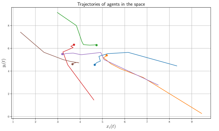
Figure 1: Trajectories in the space of agent in $\mathcal{N}$ seeking for a formation. The final achieved shape is a hexagon.

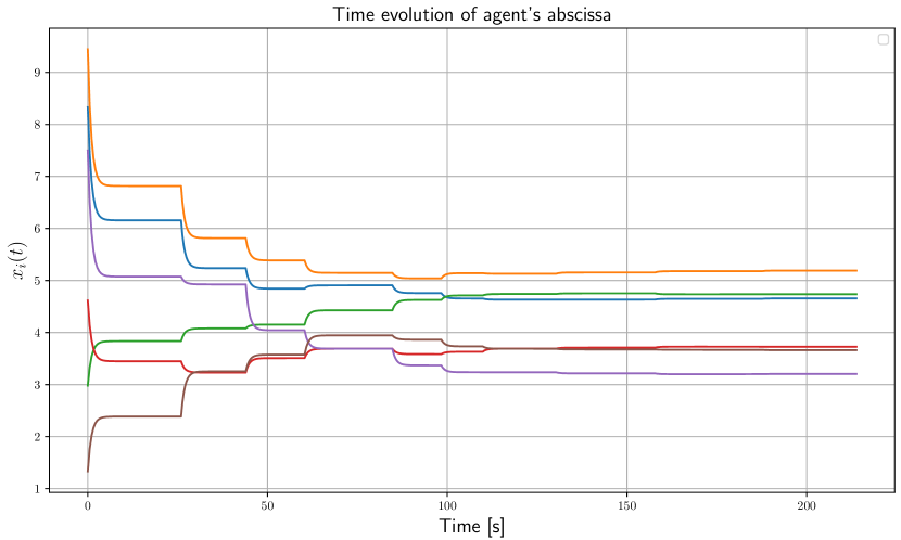
Figure 2: Evolution through time of the physical abscissa coordinate of each agent’s dynamics.

A set $\mathcal{N}$ composed of $n=6$ agents is given, where, $\forall i\in\mathcal{N}$, $x_{i}(0)$ and $y_{i}(0)$ are randomly chosen. The following parameters are used in the simulation, $\forall i\in\mathcal{N}$, $\forall k\in\mathbb{N}_{0}$, $a_{i}^{x}(t_{k})=a_{i}^{y}(t_{k})=0.5$, $b_{i}^{x}(t_{k})=b_{i}^{y}(t_{k})=0.5$, $\sigma_{i}(t_{k})=0.8$. Desired displacements from the formation centroid ($d_{i}^{x}$ and $d_{i}^{y}$) are given, so that the final desired formation is a hexagon.

A sequence of different strongly connected network topologies, i.e. $\{\mathcal{A}(k)\}_{k\in\mathbb{N}_{0}}$, is randomly chosen. At every update step $t_{k}$, $k\in\mathbb{R}_{0}$, also channel fading coefficients are randomly generated, so that, $\forall i\in\mathcal{N},\ \forall j\in\mathcal{N}_{i}(k)$, the coefficients are independent and identically distributed, $\xi_{ij}(k)\sim\mathcal{U}(0,1)$. Also, the sequence $\{\Delta(k)\}_{k\in\mathbb{N}_{0}}$ is randomly chosen, i.e., $\forall k\in\mathbb{N},\ \Delta(k)\sim\mathcal{U}(10,30)$.

Finally, simulation is run. For solving the differential equations in (10), the odeint function from Python is used. In Figure 1, the two-dimensional trajectories of agents are plotted. Clearly, they converge to the desired hexagonal formation. The evolution of the agents’ $x$-position over time is shown in Figure 2.

Also from Figure 2, one can see that, at update time $t_{7}=130\,s$, agents have basically reached the desired formation. With regards to Section VII, reaching the goal has required $g_{bc}$ orthogonal transmissions, where $g_{bc}=21$, i.e. $3$ orthogonal transmissions per $7$ update times. We compare this to the standard approach. Assume the worst case scenario which still guarantees that $\mathcal{G}(k)$ is strongly connected, $\forall k\in\mathbb{N}_{0}$, i.e. $\sum_{i=1}^{n}|\mathcal{N}_{i}(t_{k})|=10$, hence $g_{k}=20$. This shows that, in the case at hand, the amount of wireless resources used for converging with a broadcast-based protocol is equal to the amount of resources required for just one update step of the standard approach. The important amount of saved wireless resources explains why what presented in this paper constitutes an efficient formation control strategy.

IX Conclusion

In this paper, a consensus-based formation control strategy has been proposed. It guarantees that agents with single integrator continuous-time dynamics achieve the desired formation, and it exploits the superposition property of the wireless channel. This translates in having synchronized discrete-time broadcasts.

Note that the designed controller does not implement any collision avoidance strategy. This will be addressed in future work. Additionally, we aim to investigate how to extend (1) to a more general double-integrator dynamics. Furthermore, we aim at experimentally validating the proposed protocol.

References

- [1] W. Ren, R. W. Beard, and E. M. Atkins, “Information consensus in multivehicle cooperative control,” IEEE Control systems magazine, vol. 27, no. 2, pp. 71–82, 2007.
- [2] R. Olfati-Saber and R. M. Murray, “Consensus problems in networks of agents with switching topology and time-delays,” IEEE Transactions on automatic control, vol. 49, no. 9, pp. 1520–1533, 2004.
- [3] R. Falconi, L. Sabattini, C. Secchi, C. Fantuzzi, and C. Melchiorri, “Edge-weighted consensus-based formation control strategy with collision avoidance,” Robotica, vol. 33, no. 2, pp. 332–347, 2015.
- [4] W. Utschick, Communications in Interference Limited Networks. Springer, 2016.
- [5] M. Zheng, M. Goldenbaum, S. Stańczak, and H. Yu, “Fast average consensus in clustered wireless sensor networks by superposition gossiping,” in 2012 IEEE Wireless Communications and Networking Conference (WCNC). IEEE, 2012, pp. 1982–1987.
- [6] M. Goldenbaum, H. Boche, and S. Stańczak, “Nomographic gossiping for f-consensus,” in 2012 10th International Symposium on Modeling and Optimization in Mobile, Ad Hoc and Wireless Networks (WiOpt). IEEE, 2012, pp. 130–137.
- [7] F. Molinari, S. Stanczak, and J. Raisch, “Exploiting the superposition property of wireless communication for average consensus problems in multi-agent systems,” in 2018 European Control Conference (ECC). IEEE, 2018, pp. 1766–1772.
- [8] F. Molinari, S. Stańczak, and J. Raisch, “Exploiting the superposition property of wireless communication for max-consensus problems in multi-agent systems,” in 7th IFAC Workshop on Distributed Estimation and Control in Networked Systems NECSYS 2018, pp. 176–181.
- [9] J. Almeida, C. Silvestre, and A. M. Pascoal, “Continuous-time consensus with discrete-time communications,” Systems & Control Letters, vol. 61, no. 7, pp. 788–796, 2012.
- [10] M. Goldenbaum, H. Boche, and S. Stańczak, “Harnessing interference for analog function computation in wireless sensor networks,” IEEE Transactions on Signal Processing, vol. 61, no. 20, pp. 4893–4906, 2013.
- [11] M. Goldenbaum, S. Stanczak, and M. Kaliszan, “On function computation via wireless sensor multiple-access channels,” in 2009 IEEE Wireless Communications and Networking Conference. IEEE, 2009, pp. 1–6.
- [12] R. A. Horn, R. A. Horn, and C. R. Johnson, Matrix analysis. Cambridge university press, 1990.
- [13] J.-y. Shao, “Products of irreducible matrices,” Linear algebra and its applications, vol. 68, pp. 131–143, 1985.
- [14] J. Wolfowitz, “Products of indecomposable, aperiodic, stochastic matrices,” Proceedings of the American Mathematical Society, vol. 14, no. 5, pp. 733–737, 1963.
- [15] Š. Schwarz, “New kinds of theorems on non-negative matrices,” Czechoslovak Mathematical Journal, vol. 16, no. 2, pp. 285–295, 1966.
- [16] E. Seneta, Non-negative matrices and Markov chains. Springer Science & Business Media, 2006.