A Comparative Study for Unsupervised Network Representation Learning

Abstract

There has been significant progress in unsupervised network representation learning (UNRL) approaches over graphs recently with flexible random-walk approaches, new optimization objectives and deep architectures. However, there is no common ground for systematic comparison of embeddings to understand their behavior for different graphs and tasks. We argue that most of the UNRL approaches either model and exploit neighborhood or what we call context information of a node. These methods largely differ in their definitions and exploitation of context. Consequently, we propose a framework that casts a variety of approaches – random walk based, matrix factorization and deep learning based – into a unified context-based optimization function. We systematically group the methods based on their similarities and differences. We study their differences which we later use to explain their performance differences (on downstream tasks).

We conduct a large-scale empirical study considering 9 popular and recent UNRL techniques and 11 real-world datasets with varying structural properties and two common tasks – node classification and link prediction. We find that for non-attributed graphs there is no single method that is a clear winner and that the choice of a suitable method is dictated by certain properties of the embedding methods, task and structural properties of the underlying graph. In addition we also report the common pitfalls in evaluation of UNRL methods and come up with suggestions for experimental design and interpretation of results.

1 Introduction

There has been a resurgence of unsupervised methods for network embeddings for graphs in the last five years [21, 30, 19, 10]. This is primarily due to improvements in modelling and optimization techniques using neural network based approaches, and their utility in a wide variety of prediction and social network analysis tasks such as link prediction [13], vertex classification [6], recommendations [35], knowledge-base completion etc.

Lack of a comprehensive study. In spite of their success, there is a lack of an in depth systematic study of the differences between various embedding approaches. Prior works have mainly focused on studying similarities between different embedding approaches using unifying theoretical frameworks [14, 22]. As we show in our experiments (cf. Section 7), evaluation studies accompanying each new approach mostly focus on the experimental regimes where they perform well and omit the scenarios where they might perform sub-optimally. Comprehensive large-scale studies comparing these approaches under different experimental conditions are missing altogether to the best of our knowledge. Thus a fundamental practical question remains largely unanswered: From a comparative standpoint, Which Unsupervised Network Representation Learning (UNRL) approaches for nodes are most effective for different graph types and different downstream tasks?

In this paper, we fill this gap by first proposing a common framework that focuses on the differences between the various UNRL approaches. Secondly, we perform a comprehensive experimental evaluation with 9 embedding methods (cf. Table II) using different paradigms – random walks, edge modeling, matrix factorization and deep learning – that includes some of the earliest approaches for learning network representations to the more recent deep learning based approaches and 11 datasets (cf. Table III). In this work we consider only unsupervised methods in the transductive scenario.

Unifying framework. Our common framework for understanding UNRL approaches is inspired by the observation that most of the unsupervised learning approaches operate on an auxiliary neighborhood graph in which similar vertices share an edge. We call such a graph a context graph and for any source vertex $v$, its one-hop neighbor is called its context. Depending on the embedding method, a vertex can be in the context of another if they are in the immediate neighborhood, reachable by truncated random walks, or if they are in the same community/cluster etc. In this paper we study a wide variety of approaches– e.g. that employ random walks [21, 6, 37, 30], neighborhood modelling [28], matrix factorization [22, 19] and deep learning [7, 32] – in our unified framework, where these methods can be understood as optimizing a common form of objective function defined on their respective context graphs. This allows us to understand the differences among these approaches that arises due to their modelling of context.

Comprehensive Experimental Evaluation. In our evaluation of UNRL methods we investigate the conceptual differences between the embedding approaches that result in performance differences on downstream tasks. First, using graphs with diverse structural characteristics we argue about the utility of several approaches. We carefully chose 11 large network datasets (5 undirected and 6 directed) with diverse properties from social networks, citation networks, and collaboration networks. With focus on reproducibility and large scale analysis, we chose at least one dataset used in each of the original papers and try to be as close to the authors original experimental setup as possible on four popular tasks – node classification, link prediction, clustering and graph reconstruction. The first two tasks are thoroughly investigated in the main paper and all details corresponding to clustering and graph reconstruction tasks are only provided in the supplementary material. Second, in addition to performing a large-scale study with a large number of baselines we also find limitations in the experimental setup of earlier approaches. In particular, for evaluating link prediction performance in case of directed graphs most of the earlier works only check for the existence of an edge between a pair of nodes and ignore directionality of the edge. Finally, we question the claimed superiority of various embedding methods in the node classification task, wherein a naïve (yet effective) baseline is not considered. We surprisingly find that for several of the datasets comparable or even better performance is achieved by our improved naïve baseline.

Key findings. Our study does not propose a winner or a loser but highlights the strengths and weaknesses of approaches under different graph and task characteristics. We believe that our results can serve as guidelines for researchers and industry practitioners in the choice of the wide range of embedding methods considered in this work. Some of the key findings of our study are as follows:

• Methods respecting the vertex’s role as source and context during learning of representations as well as in their use for a task are recommended for link prediction in directed graphs.

• Certain structural properties like clustering coefficient, transitivity, reciprocity etc. are recommended to be considered while choosing a specific method.

• A simple immediate neighborhood based classifier turns out to be offering better or comparable performance for a number of datasets.

2 Related Work

With increasing number of unsupervised embedding methods, it has become extremely difficult to objectively compare and choose appropriate methods for a given dataset. Several existing surveys focus on categorization of various network embedding techniques with respect to the methodology such as random walks, matrix factorization and edge modeling etc [2, 3]. But they fail to provide any unifying framework to compare and gain deeper understanding of various methods. Other works which do provide a common framework only focus on demonstrating the equivalence of various methods to matrix factorization [14, 22, 34] but do not consider the differences between the methods and their impact on task performance for a variety of graphs with different structural properties. Several other surveys [8, 33] consider a wide range of unsupervised and semi-supervised embedding methods without any empirical comparison. More importantly, the categorization and comparison in these surveys does not directly correspond with explaining why some methods are superior to other methods under certain circumstances. Surveys which include empirical comparison [5, 36] focus only on effect of training data size for various tasks or the effect of varying hyperparameters on task performance. In [24], the authors consider semi-supervised node classification and demonstrate the effect of different train/validation/test splits and hyperparameters on the performance of several graph neural network models.

We remark that the scope of this work includes unsupervised, transductive methods and non-attributed graphs. We include the most popular representative methods which follow our common objective function in our study. Other methods, for example based on generative modelling [11], adversarial training [20], uncertainty modelling [1] do not fall under our context based formulation and each of these categories deserves a separate study. Semi-supervised methods like graph attention networks [31] are also not considered in our study.

3 Unifying Framework and Research Questions

In this section we first build a unifying framework in which we can conveniently cast the objective functions of the random walk, matrix factorization and deep learning based Unsupervised Network Representation Learning (UNRL) methods. In particular, given a graph $G=(V,E)$ we are interested in learning low dimensional representations of each node $v\in V$ such that similar nodes in $V$ are embedded closer. These representations are then used for downstream tasks for example predicting missing links in $G$ or in node classification task where the goal is to predict missing node labels. Note that as we do not consider additional node or edge attributes in this work, the similarity information among the vertices is inferred from the topological structure of $G$. Towards defining our common framework, we introduce the notion of a context graph and propose a common objective function into which all of the methods under investigation can be mapped.

3.1 Context Graph

In order to understand how various methods differ in their definitions and treatment of similarity, we begin by constructing an auxiliary directed and weighted graph $\mathcal{C}$ from $G$ where $\mathcal{C}=(V,E^{\prime})$ such that the higher the weight of edge $(u,v)\in E^{\prime}$ the larger the similarity among nodes $u$ and $v$. Moreover for nodes with no edge between them, we construct an edge with weight $-1$. The negative weight here denotes the dissimilarity between two nodes. We call $\mathcal{C}$ as the context graph and for each edge $(u,v)\in E^{\prime}$, $v$ is called the context of node $u$. Let $C$ denote the corresponding adjacency matrix of $\mathcal{C}$ with $c_{i,j}$ denoting $(i,j)th$ element in $C$. For an edge $(u,v)\in E^{\prime}$, we call $u$ as the source node and $v$ its context.

As each node can be a source or a context of some other node, we denote the source and context representations of nodes in $\mathcal{C}$ by $\Phi\in\mathbb{R}^{|V|}\times\mathbb{R}^{d}$ and $\theta\in\mathbb{R}^{|V|}\times\mathbb{R}^{d}$ respectively. For any node $v_{i}$, $\Phi_{i}$ and $\theta_{i}$ represent respectively its d-dimensional source and context vectors (representations). We are then interested in learning $\Phi$ and $\theta$ while minimizing the following loss

$$\mathcal{J}=-\sum_{i,j}c_{i,j}\cdot f(\Phi_{i},\theta_{j}),$$ (1)

where, $f$ is monotonically increasing in $\Phi_{i}\cdot\theta_{j}$.

We recall that by our construction, for any two dissimilar nodes $i,j$, $c_{i,j}=-1$. This imposes an additional constraint on the embedding vectors such that the corresponding dot product of embedding vectors is minimized for dissimilar nodes. Note that by minimizing (1) a vertex (in its source representation) will be embedded closer to its context (in its context representation); and therefore two vertices sharing same context will be embedded closer (in their source representations) by transitivity. In this work we consider DeepWalk [21], Node2vec [6], APP [37], LINE-2 [28] employing the above form of the loss function. We also include two methods which use matrix factorization objectives–HOPE [19] and NetMF [22], based on their equivalence to the above objective demonstrated in [14].

In some works such as Verse [30], LINE-1 [28], SDNE [32], unsupervised GraphSAGE [7] the loss function does not consider separately the context role of a vertex. More specifically, for any two neighboring nodes they attempt to embed vertices closer by maximizing the dot product of their source representations. Formally, they learn only $\Phi$ by minimizing the following loss function.

$$\mathcal{J^{\prime}}=-\sum_{i,j}c_{i,j}\cdot f(\Phi_{i},\Phi_{j}).$$ (2)

While many of the considered methods can be explained under a unified framework based on their similarities in their objective functions (as also done by previous works [22, 14]), we are interested in understanding their differences due to their modelling decisions.

Symbol/ Text	Meaning
$G$	Undirected or directed graph with vertex set $V$ and edge set $E$
$\mathbf{P}=D^{-1}A$	Transition matrix where A and D are the adjacency and degree matrices of $G$
$d_{i}$	out-degree of a vertex $v_{i}$ in $G$
$\mathcal{C}$	Context graph of $G$
$C$	Adjacency matrix of $\mathcal{C}$
context	One-hop neighbor of a vertex in $\mathcal{C}$
$\Phi,\theta$	Source and Context representation matrices

TABLE I: Notations

Context Graph	Algorithm	Sym. C	Learnt Embeddings	Used Embeddings	Loss	Optimization
Random Walk based	DeepWalk	✓	$\Phi,\theta$	$\Phi$	$-\sum_{i,j}c_{i,j}\log{\exp{(\Phi_{i}\cdot\theta_{j})}\over\sum_{k\in V}\exp(\Phi_{i}\cdot\theta_{k})}$	Hierarchical Softmax
Random Walk based	Node2vec	✓	$\Phi,\theta$	$\Phi$	$-\sum_{i,j}c_{i,j}\log{\exp{(\Phi_{i}\cdot\theta_{j})}\over\sum_{k\in V}\exp(\Phi_{i}\cdot\theta_{k})}$	Negative Sampling (NS)
PPR based	APP	✗	$\Phi,\theta$	$\Phi,\theta$	$-\sum_{i,j}c_{i,j}\log{\exp{(\Phi_{i}\cdot\theta_{j})}\over\sum_{k\in V}\exp(\Phi_{i}\cdot\theta_{k})}$	NS
PPR based	Verse	✗	$\Phi$	$\Phi$	$-\sum_{i,j}c_{i,j}\log{\exp{(\Phi_{i}\cdot\Phi_{j})}\over\sum_{k\in V}\exp(\Phi_{i}\cdot\Phi_{k})}$	NS
Adjacency based	LINE-1	✓	$\Phi$	$\Phi$	$-\sum_{i,j}c_{i,j}\log{1\over 1+\exp(-\Phi_{i}\cdot\Phi_{j})}$	NS
Adjacency based	LINE-2	✗	$\Phi,\theta$	$\Phi$	$-\sum_{i,j}c_{i,j}\log{\exp{(\Phi_{i}\cdot\theta_{j})}\over\sum_{k\in V}\exp(\Phi_{i}\cdot\theta_{k})}$	NS
Direct matrix	NetMF	✗	$\Phi,\theta$	$\Phi$	$||C-\Phi\cdot\theta||^{2}_{F}$	Matrix Factorization (MF)
Direct matrix	HOPE	✗	$\Phi,\theta$	$\Phi,\theta$	$||C-\Phi\cdot\theta||^{2}_{F}$	MF
Adjacency based	SDNE	✗	$\Phi$	$\Phi$	see Equation (10)	Deep Autoencoders
Random Walk based	Unsupervised GraphSAGE	✓	$\Phi$	$\Phi$	$-\sum_{i,j}c_{i,j}\log{\exp{(\Phi_{i}\cdot\Phi_{j})}\over\sum_{k\in V}\exp(\Phi_{i}\cdot\Phi_{k})}$	NS with Neighborhood Aggregation

TABLE II: A summary of Network Representation Learning algorithms with respect to Context and Optimization. Sym.C corresponds to if the adjacency matrix of context graph is symmetric .

In the rest of this section, we elaborate these differences based on (1) how they define context or neighborhood in the corresponding context graph, (2) how they exploit context and (3) how they optimize their objectives. In Section 3.2 we list 4 different schemes of defining context with each scheme having examples of two embedding methods. For these chosen methods, we then focus on exploitation of context in Section 3.3. We then elaborate on various optimization approaches used by these methods in Section 3.4. The main discussed differences and similarities among the studied methods is also summarized in Table II. Finally, in Section 3.5, we formulate a set of research questions which are answered based on the differences elaborated below and the experimental results in Section 7. The main notations used in the rest of the paper are listed in Table I.

3.2 Different Schemes of Defining Context

In this section, we compare various approaches with respect to the different ways in which the context graph is defined in Section 3.1. The simplest possible context matrix which can be used is the adjacency matrix itself, i.e., nodes sharing a link are similar to each other. In this case the context graph is the same as the original graph $G$. While some methods directly use similarity notions like Katz similarity [9] (e.g., HOPE) or Personalized PageRank (e.g., Verse) to quantify similarity among vertices, other methods explore higher order neighborhoods via random walks and quantify similarity among nodes by their co-occurrence in these walks (e.g., DeepWalk and Node2vec).

3.2.1 Random Walk Based Context

In random walk based methods, the higher order neighborhoods are usually sampled to define the context graph. Roughly, a vertex pair $(u,v)$ co-occurring in a random walk will correspond to two directed edges in the context graph : $u\rightarrow v$ and $v\rightarrow u$. In the first edge $v$ serves as a context for $u$ while for the second edge $u$ is the context. We explain below more precisely the context graphs of two popular methods under this category, namely DeepWalk and Node2vec.

DeepWalk, Node2vec . These methods employ truncated random walks of length $T$ from each vertex $v\in V$ to create vertex sequence, say $W_{v}$. In particular, for each $v_{i}\in W_{v}$ and for each $v_{j}\in W_{v}[i-r:i+r]$ (r is the window size), $(v_{i},v_{j})$ forms an edge in the corresponding context graph. While DeepWalk performs a uniform random walk, Node2vec follows a 2nd order random walk.

More specifically, from [22], for any pair of vertices $v_{i},v_{j}\in V$ for DeepWalk’s walk lengths $T$ and window size $r$ we have

$${c_{i,j}\over\sum_{u,v|c_{u,v}>0}c_{u,v}}\xrightarrow{p}{1\over 2T}\sum_{r=1}^{T}\left({d_{i}\over\sum_{i}d_{i}}\cdot(\mathbf{P}^{r})_{i,j}+{d_{j}\over\sum_{i}d_{i}}\cdot(\mathbf{P}^{r})_{j,i}\right),$$ (3)

Note that the ratio in the L.H.S of (3), i.e. the ratio of weight of edge $(v_{i},v_{j})$ to the total (positive) edge weight in the context graph, quantifies the similarity of vertices $v_{i}$ and $v_{j}$. The similarity between $v_{i}$ and $v_{j}$ is therefore proportional to the sum of probabilities that vertex $v_{j}$ is reachable from a $r$-truncated random walk started from the vertex $v_{i}$ and vice versa. Here $r$ varies from $1$ till the original walk length $T$. One of the implications of (3) is that $c_{i,j}$ and $c_{j,i}$ both represent exactly the same quantity as the r.h.s is symmetric in $i$ and $j$. In general the probability of reaching $v_{i}$ to $v_{j}$ by a random walk of $r$ hops i.e. $(\mathbf{P}^{r})_{i,j}$ is not the same as the probability of reaching from $v_{j}$ to $v_{i}$ in $r$ hops ($(\mathbf{P}^{r})_{j,i}$), the presence of both the terms in r.h.s make the similarity between source $v_{i}$ and context $v_{j}$ equal to similarity between source $v_{j}$ and context $v_{i}$. Therefore, even if the context is explicitly represented by learning a context representation for each node, the possible asymmetric properties of source and context are completely ignored. For example, consider two vertices in a directed graph or in an undirected graph with very different local neighborhood structures such that the reachability probability of one node to another is not the same in the other direction.

Considering the biased walks in Node2vec, it first computes a second order transition probability to sample the next vertex in the walk as defined below.

$$\mathbf{\underline{P}}_{u,v,w}={T_{u\rightarrow v\rightarrow w}\over\sum_{w}T_{u\rightarrow v\rightarrow w},}$$

where

$$T_{u\rightarrow v\rightarrow w}=\begin{cases}{1\over p},\text{if }(u,v)\in E(v,w)\in E,u=w\\ {1},\text{if }(u,v)\in E(v,w)\in E,u\neq w,(u,w)\in E\\ {1\over q},\text{if }(u,v)\in E(v,w)\in E,u\neq w,(u,w)\not\in E\\ 0,\text{otherwise}\end{cases}.$$ (4)

From (4), we note that for directed graphs where an edge $(u,v)$ does not automatically apply existence of an edge $(v,u)$, $p$ might have limited or no influence over the random walks, for example for directed graphs with zero reciprocity. Again for graphs with low clustering coefficient, condition 2 might not hold for many cases. In summary, biased walks of Node2vec might be reduced to uniform random walks as employed by DeepWalk for graphs with low reciprocity and low clustering coefficient and transitivity.

Under assumptions of infinite length walks on undirected graphs, it can be shown that for Node2vec

$${c_{i,j}\over\sum_{u,v|c_{u,v}>0}c_{u,v}}\xrightarrow{p}{1\over 2T}\sum_{r=1}^{T}\sum_{k}\left({\mathbf{X}_{k,i}}(\mathbf{\underline{P}}^{r})_{k,i,j}+{\mathbf{X}_{k,j}}(\mathbf{\underline{P}}^{r})_{j,k,i}\right),$$ (5)

where $\mathbf{X}$ represents a stationary distribution of the second order random walk. Comparing it with (3), uniform degree distribution to choose the source vertex and the transition probabilities are respectively replaced with stationary distribution of the second order random walk and the second order transition probability. As (5) is again symmetric in $i,j$, we also obtain a symmetric adjacency matrix for context graphs used by Node2vec. In summary, the respective context graphs have the following properties.

Property 1.

For DeepWalk and Node2vec’s context graphs, the roles of a vertex as source and context are indistinguishable by construction, for example $c_{i,j}$ and $c_{j,i}$ will be identical even if the underlying graph $G$ is directed.

Property 2.

The parameter $p$ as used by Node2vec will have no effect for a directed graph with zero reciprocity as there are no back edges.

Property 3.

For any triplets $u,v,w$ we have $\mathbf{P}_{v,w}=\mathbf{P}_{u,v,w}$ when $u,v,w$ do not form a triangle and there are no back edges, i.e., $u\neq w$. This implies that Node2vec’s biased walks might not give any additional advantage in case of graphs with low transitivity, low clustering coefficient and zero reciprocity.

3.2.2 Personalized PageRank (PPR) Based Context

APP and Verse. These methods use random walks with restarts to draw source-context pairs. In particular, every time a walk starts from a vertex chosen uniformly at random; a walk is continued with probability $1-\alpha$ where $\alpha$ is the predefined restart probability. The first and last vertices of this walk forms a directed edge in the corresponding context graph with the first node of the walk being the source node. For any vertices $i,j\in V$ we compute the theoretical estimate of $c_{i,j}\over\sum_{u,v}c_{u,v}$.

Proposition 1.

Let $i\in V$ be uniformly chosen as done in APP. Let $j\in V$ be such that the shortest hop distance between nodes $i$ and $j$ be $h$. Then node $j$ is the last node in the walk starting from $i$ with probability $O({1\over|V|}(1-\alpha)^{h}\cdot\alpha\cdot(\mathbf{P}^{h})_{i,j})$, i.e.,

$${c_{i,j}\over\sum_{u,v|c_{u,v}>0}c_{u,v}}=O\left({1\over|V|}(1-\alpha)^{h}\cdot\alpha\cdot(\mathbf{P}^{h})_{i,j}\right).$$

The proof for above proposition is provided in the supplementary material. We observe that the context graph used by APP and Verse is considerably different from that used by DeepWalk and Node2vec. Note Equations (3) and (5) imply $c_{i,j}=c_{j,i}$ for DeepWalk and Node2vec whereas this is not the case for APP and Verse, where their values depend on the neighborhood structures of nodes as shown in Figure 1 where there is a higher probability of reaching from node $u$ to $v$ than vice-versa. We therefore have the following property.

Property 4.

For any $i,j\in V$, $c_{i,j}$ is not always equal to $c_{j,i}$, i.e., $C$ is not always a symmetric matrix or the similarity relation between vertices is not always symmetric.

3.2.3 Adjacency Based Context

LINE  and SDNE. These methods directly use the given graph as its context graph, i.e., $C=A$. They aim to embed vertices closer which have either links between them (optimizing for first order proximity) or share common 1-hop neighborhood (optimizing for second order proximity). They specifically differ in their exact formulations of loss functions and optimization strategies which will be discussed in detail in Section 3.4. Corresponding to LINE, we study both of its variants : LINE-1 ( optimizing only first-order proximity) and LINE-2 (optimizing only second-order proximity). LINE-1+2 is obtained by normalizing and concatenating the embedding vectors from LINE-1 and LINE-2

Special Case of Unsupervised GraphSAGE. GraphSAGE uses a two layer deep neural architecture where in each layer $k$ a node $v\in V$ computes its representation $h^{k}$ as an aggregation of representations (from previous layer) of its neighbors, $\{h^{(k-1)}(u),\forall u\in N(v)\}$. The parameters of aggregation functions are learnt using the loss function similar to DeepWalk. In other words, GraphSAGE also optimizes for embedding the vertices closer, which are more similar with respect to the context matrix generated using Equation (3), where, an source embedding vector of a vertex is a function of embedding vectors of its immediate neighbors. Intuitively this implies that vertices having links between them will be embedded closer. For GraphSAGE we report the best results corresponding to one of its four aggregators (Mean, MeanPool, MaxPool and LSTM). In addition, we study GCN variant of GraphSAGE where the aggregator function is the graph convolution network. Note that we used the unsupervised and transductive variant of GraphSAGE for this work.

3.2.4 Direct Matrix Based Context

NetMF. NetMF is derived from a theoretical analysis of DeepWalk and directly factorizes the context matrix with $(i,j)$th element given by

$$c_{i,j}=\log\left({vol(G)\over kT}\left({1\over d_{j}}\cdot{(\sum_{r=1}^{T}\mathbf{P}^{r}})_{i,j}\right)\right)$$ (6)

where $T,r,k$ are hyperparameters and correspond to walk length, window size and negative samples in DeepWalk.

We remark here that while DeepWalk explicitly encodes similarity between vertices as given by Equation (3), using the equivalence of SGNS[15] optimization to matrix factorization, [22] proposes that DeepWalk implicitly factorizes the context matrix with its $(i,j)th$ element given by Equation (6). Note that the focus of this work is not to validate/invalidate this connection but understand the kind of vertex similarities different methods try to encode in its latent representations. DeepWalk and NetMF are therefore not only different from their optimization techniques but also their respective context graphs representing similarities between vertices.

HOPE. This approach preserves the asymmetric role information of the nodes by approximating high-order proximity measures like Katz measure [9], Rooted PageRank [26] etc. We study the version of HOPE where it uses Katz similarity matrix as the context matrix as it also gives us a different type of context graph to compare with. For example, the context graph generated for Rooted PageRank is quite similar to the ones used by Verse and APP. In a Katz similarity matrix, each entry $c_{i,j}$ is a weighted summation over the path set between two vertexes. More specifically, $c_{i,j}=\sum_{\ell=1}^{\infty}\beta^{k}(A^{k})_{i,j},$ where $\beta$ is a decay parameter and determines how fast the weight of the path decay with growing length.

3.3 Exploitation of Context

Methods differ in their learning and usage of context representations. While some methods only learn source representation for a node, other methods learn both representations but only utilize source representations for the downstream task. There is yet another class of methods which in addition to learning two representations also use both of them for downstream tasks.

DeepWalk, NetMF, LINE-2 and Node2vec. These methods learn both source and context representations but use only source representation for the downstream tasks.

GraphSAGE, LINE-1, Verse and SDNE. All of these methods learn only a source representation of a vertex and ignore its representation as a context.

APP and HOPE. Both these methods learn two representations per vertex and use both the representations for downstream tasks. They in fact use the context representation to represent the node in its destination role if the original graph $G$ is directed.

Difference between APP and Verse. APP and Verse both perform random walks with restarts to compute their respective context graphs. As already discussed (cf. Property 4), the similarities encoded by the context graph in their case are not symmetric, yet Verse ignores this asymmetries and attempts to encode the similarities between vertices in a single embedding space. This is quite contrary to its motivation of encoding Pensonalized PageRank (PPR) which is by construction asymmetric, i.e., $PPR(i,j)$ is not always equal to $PPR(j,i)$, where $PPR(i,j)$ represents the PPR of $i$ with respect to $j$ .

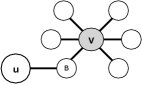
Figure 1: Asymmetric local structures in Undirected Graphs

3.4 Differences in Optimization Methods

Optimization methods span from direct matrix factorization, deep autoencoders, negative sampling to neighborhood aggregation methods using convolutions.

Hierarchical softmax [17] and Negative Sampling [15]. DeepWalk, Node2vec, LINE-2, APP model $f$ in Equation (1) as logarithm of probability for pair $(i,j)$ sharing an edge in the context graph, i.e.,

$$f(\Phi_{i},\theta_{j})=\log{\exp(\Phi_{i}\cdot\theta_{j})\over\sum_{k}\exp(\Phi_{i}\cdot\theta_{k})}$$ (7)

Verse uses exactly the same form of $f$ except that it uses only source representation, i.e, it defines $f$ as

$$f^{verse}(\Phi_{i},\Phi_{j})=\log{\exp(\Phi_{i}\cdot\Phi_{j})\over\sum_{k}\exp(\Phi_{i}\cdot\Phi_{k})}$$ (8)

Since exact computation of $f$ would require computations over all vertex-pairs which would be very expensive. Instead these methods make use of approximations namely hierarchical softmax and negative sampling. Hierarchical softmax is only used by DeepWalk. Other methods employ negative sampling.

For LINE-1, the corresponding function is given as

$$f^{LINE1}(\Phi_{i},\Phi_{j})=\log{1\over 1+\exp(-\Phi_{i}\cdot\Phi_{j})}$$ (9)

and it further approximates it using negative sampling.

Neighborhood Aggregation and Negative Sampling. GraphSAGE trains a set of aggregator functions that learn to aggregate feature information from a vertex’ local neighborhood. Like other methods, GraphSAGE uses an unsupervised loss and its context graph corresponding to the loss function is same as that of DeepWalk. Instead of directly learning the embeddings as done by other methods, GraphSAGE learns the parameters of the aggregator functions via stochastic gradient descent.

Deep Autoencoders. SDNE uses a multi-layer auto-encoder model to capture non-linear structures based on first- and second-order proximities. By reconstructing first order proximity, the model aims to embed vertices closer which have links between them with the corresponding loss function given by $\mathcal{L}_{1}=\sum_{i,j}c_{i,j}||\Phi_{i}-\Phi_{j}||^{2}$.

Drawing parallel to (2) we have $f^{SDNE}=-||\Phi_{i}-\Phi_{j}||^{2}$. For preserving second order proximity it uses the adjacency matrix as input to the autoencoder. Denoting row $i$ of matrix $C$ by $c_{i}$ the reconstruction process will make the vertices with similar neighborhood structures have similar latent representations, i.e, the following loss function will be minimized: $\mathcal{L}_{2}=\sum_{i}||c_{i}-g(\Phi_{i})\odot\beta||^{2}$. where $g$ is a decoder function. $\mathcal{L}_{2}$ is an auxiliary reconstruction loss and is restricted to a node rather than a pair of nodes and hence is of different form than Equation (2).

The contribution of these two proximities is controlled by the hyperparameter $\alpha$ such that setting $\alpha=0$ will switch to only preserving second order proximity. Another hyperparameter $\beta$ controls the reconstruction of zero elements in the adjacency matrix of the training graph. For simplicity we state the loss function without the regularization term:

$$\mathcal{J}=\mathcal{L}_{2}+\alpha\mathcal{L}_{1}$$ (10)

Remark 1.

Like SDNE, LINE also aims to preserve first and second order proximities. But unlike LINE, SDNE uses a deep neural network and performs joint optimization as opposed to learning two separate embeddings and later concatenating them.

Matrix Factorization. HOPE and NetMF compute low rank decomposition of their respective context matrices. While HOPE uses both factors for downstream task denoting the first factor as the source representation of the vertex and the second as target representation, NetMF only uses one representation matrix for downstream tasks. Their loss function is given as: $\mathcal{J}=||C-\Phi\cdot\theta||_{F}^{2}$, where $||.||_{F}$ denotes the Forbenius norm.

Table II summarizes the list of embedding methods along with the corresponding properties with respect to defining and exploiting context and loss functions.

3.5 Research Questions

Based on the differences due to context and optimization methods, we formulate the following research questions.

RQ 1.

How does the choice of different context schemes defined in Section 3.2 affect the performance of downstream tasks? And to what extent is this performance influenced by the structural properties of the underlying graph?

RQ 2.

How do different ways of exploiting the context listed in Section 3.3, affect the performance of network representation learning methods? Which combination of downstream tasks and input graphs could benefit from the explicit use of context embeddings?

RQ 3.

How does the choice of optimization method (listed in Section 3.4) affect the performance? Do deep models always outperform the shallow models?

We answer these research questions in Section 7 based on the observations from extensive experimental comparison and summarize the answers in Section 7.3.

4 Task Description

In this section we describe the two most popular tasks used for empirically comparing various UNRL methods – Link Prediction (LP) and Node Classification (NC). We also discuss the shortcomings of previous works with respect to these tasks and propose new experimental settings to overcome the same. We also considered Graph Reconstruction (GR) and Graph Clustering (GC), please refer to the supplementary material (Sections 4 and 5) for details.

4.1 Link Prediction (LP)

The aim of the link prediction task is to predict missing edges given a network with a fraction of removed edges. In the literature there have been slightly different yet similar experimental settings. A fraction of edges is removed randomly to serve as the test split while the residual network can be utilized for training. The test split is balanced with negative edges sampled from random vertex pairs that have no edges between them. While removing edges randomly, we make sure that no vertex is isolated, otherwise the representations corresponding to these vertices can not be learned.

For directed graphs in addition to the existence of an edge it is also desirable to learn about the directionality of the edge. Therefore, for directed graphs we inverse a fraction of positive edges in the test split in order to create negative edges. For example given an edge $(a,b)$ in the test split we check if $(b,a)$ is also an edge. If not, we replace another negative edge with $(b,a)$ in the negative edge list of the test split. It is trivial to note that methods using only the source representation would not be able to simultaneously predict the existence of edge $(a,b)$ and non existence of edge $(b,a)$.

Tables IV and V present the ROC-AUC (Area Under the Receiver Operating Characteristic Curve) scores for undirected and directed graphs respectively. For each method, the inner product of representation of the pair of vertices normalized by the sigmoid function is employed as the similarity/link-probability measurement.

Remark 2.

We remark that most of the previous works are lacking in the sense that they only evaluate if the method predicts a link and ignore the edge directionality for directed graphs hence giving an unfair treatment to methods designed specifically for directed graphs like HOPE and APP.

Remark 3.

Note that the difficulty of link prediction in directed graphs will be influenced by its reciprocity.

4.2 Multilabel Node Classification (NC)

Given a graph, each node has one or more labels. We report the Micro-F1 and Macro-F1 scores after a $5$-fold multi-label classification using one-vs-rest logistic regression. The main motivation behind using embeddings for this task is the assumption that the local vertex neighborhood dictates its labels. For example, a republican would have more republican than democrat friends. We use 5 undirected and 3 directed networks for this task. The three directed networks with labels are the citation networks wherein an edge represents a citation relationship.

New Baseline. In order to better judge the difficulty of predicting labels for a particular graph we propose an improved naïve baseline, which we call, Max-Vote. In this approach, in order to assign a label to a vertex, only the labels of its immediate neighbors from the training set are considered. In Max-Vote, we first split the datasets into training and test set (80-20) and the labels are assigned for the vertices in the test set using only the labels of the neighbors which are part of the training set. For a given node with $k$ labels in the ground truth, we assign it the most frequent $k$ labels of its labelled immediate neighbors. If less than $k$ neighboring nodes are labelled or the vertex’ neighbors have less than $k$ labels, remaining labels are chosen randomly from the list of all possible labels in the graph. The pseudo-code for the subroutine to label a vertex is shown in Algorithm 1 where $\ell$ denotes the total number of label classes.

Remark 4.

By homophily in node classification we understand that similar nodes share the same label. Our baseline method Max-Vote quantifies homophily when similarity is limited to similarity between immediate neighbors.

1:function Max-Vote($v,N(v),k$)

2:     for $(i=0,1,\ldots\ell)$ do

3:         $L(i)=0$      

4:     for $(i\in N(v))$ do

5:         if ($i$ is labelled) then

6:              for $j\in labels(i)$ do

7:                   $L(j)=L(j)+1$                             

8:     Choose the most frequent $k$ labels in $L$ to label $v$

Algorithm 1 Subroutine to label a node with Max-Vote

5 Structural Properties

In order to quantify the impact that different kinds of graphs have on the performance of the vertex representations, we consider diameter, reciprocity, clustering coefficient, transitivity and spectral separation.

In order to compute diameter ($D$), edge directions are not considered. In networks that are not connected, the diameter of the largest connected component is reported. In a directed network, the reciprocity ($r$) equals the proportion of edges for which an edge in the opposite direction exists, i.e., that are reciprocated. More formally, $r=\frac{1}{m}|\{(u,v)\in E\mid(v,u)\in E\}|$.

The local clustering coefficient of a vertex quantifies how probable it is for $v$ to form a clique of size $3$ with its neighbors. Formally, if $d(v)$ is the degree of $v$, then local clustering coefficient of $v$ is defined as

$$c(u)={|(u,w)\in E\mid(u,v)\in E,(v,w)\in E|\over{d(v)\choose 2}}.$$

For directed graphs, the local clustering coefficient of a vertex $u$ equals the proportion of directed 2-paths starting from $u$ that are completed by a third edge oriented in the same direction as the 2-path. The clustering coefficient ($clus$) of graph $G$ is then defined as the average of the local clustering coefficients of its vertices. We denote the directed clustering coefficient by $clus_{dir}$.

Transitivity ($T$) measures the extent to which two nodes are related in a network that are connected by an edge. It is defined as the ratio of the number of vertex triplets forming a triangle to the total number of triads (subgraphs of $3$ vertices). For directed graphs, the transitivity ($T_{dir}$) equals the proportion of directed 2-paths that are completed by a third edge oriented in the same direction as the 2-path.

The spectral separation ($S$) is the largest absolute eigenvalue of the adjacency matrix divided by the second largest absolute eigenvalue. Low values (slightly larger than one) indicate many independent substructures in the network.

6 Experimental Setup

We empirically validate the impact of various differences among the 9 embedding methods (cf. Table II) on task performance. For reproducibility we used the authors’ implementations whenever available and performed hyperparameter tuning whenever applicable. We provide a detailed description of parameter settings, hardware and software setup in the supplementary material (Section 2). We consider six social network graphs, four citation networks and an authorship network with their structural properties summarized in Table III. We consider two tasks LP and NC defined in Section 4. We also consider Graph Reconstruction and Graph Clustering tasks. However, due to lack of space their results are discussed in the supplementary material (Sections 4 and 5).

Category	Dataset	Type	$|V|$	$|E|$	$|\mathcal{L}|$	$r$	$D$	$clus$	$T$	$clus_{dir}$	$T_{dir}$	$S$
Social	BlogCatalog [29]	undir.	10K	333K	39	n.a	5	0.463	0.0914	n.a	n.a	2.18
	Flickr [29]	undir.	80K	5.90M	195	n.a	6	0.165	0.1875	n.a	n.a	2.06
	Youtube [16]	undir.	1.13M	2.99M	47	n.a	21	0.080	0.0062	n.a	n.a	1.19
	Reddit [7]	undir.	231K	11.6M	41	n.a	10	0.169	0.0458	n.a	n.a	1.47
	Twitter [4]	dir.	465K	834K	n.a	0.3%	8	0.0006	0. 0152	0.0002	0.013	1.05
	Epinion [23]	dir.	75K	508K	n.a	40.52%	15	0.1378	0.0657	0.0982	0.0902	1.74
	DBLP-Ci [12]	dir.	12.5K	49K	n.a	46.4%	10	0.1169	0.0620	0.039	0.0967	1.39
Citation	CoCit [25]	dir.	44K	195K	15	0%	25	0.1419	0.0806	0.0826	0.0913	1.07
	Cora [27]	dir.	23K	91K	70	5.00%	20	0.2660	0.1169	0.169	0.221	1.03
	PubMed [18]	dir.	19K	44k	3	0.07%	18	0.0602	0.0537	0.0325	0.0530	1.14
Collaboration	DBLP-Au [28]	undir.	1.2M	10.3M	n.a	n.a	24	0.635	0.1718	n.a	n.a	1.0005

TABLE III: A summary of benchmark datasets with properties : number of nodes ($|V|$), number of edges ($|E|$), number of labels ($|\mathcal{L}|$), reciprocity ($r$), diameter ($D$), clustering coefficient ($clus$), transitivity ($T$), directed clustering coefficient ($clus_{dir})$ and transitivity ($T_{dir}$), spectral separation ($S$). ’n.a’ indicates the specific property is ’not applicable’ to the corresponding graph.

With respect to datasets, BlogCatalog, Flickr and Youtube are social networks with users as nodes and friendship between them as undirected edges with multiple labels per node. Twitter  and Epinion  are unlabelled, directed graphs modeling the follower and trust between users respectively. DBLP-Ci, CoCit, Cora, PubMed are directed graphs representing academic citation networks, with vertices as papers and edges representing the citations between them. DBLP-Au is a collaboration network of authors of scientific papers from DBLP Computer Science bibliography. An elaborate description about the datasets can be found in the Supplementary material.

7 Results and Discussion

method	BlogCat.	Youtube	Reddit	DBLP-Au	Flickr
DeepWalk	0.527	0.586	0.897	0.850	0.772
Node2vec	0.556	0.652	0.892	0.949	0.821
Verse	0.878	0.884	0.973	0.994	0.918
APP	0.790	0.871	0.974	0.994	0.928
NetMF	0.659	✗	0.949	✗	0.604
LINE-1+2	0.612	0.894	0.949	0.989	0.839
LINE-1	0.495	0.758	0.947	0.989	0.830
LINE-2	0.400	0.823	0.833	0.896	0.694
GraphSage	0.619	0.778	0.936	0.912	0.734
GSage(GCN)	0.661	0.813	0.941	0.975	0.779
SDNE	0.519	✗	✗	✗	0.483

TABLE IV: Link prediction results for undirected graphs using 50% edges as training data. ✗ indicates the corresponding method failed to finish for the given dataset.

7.1 Link Prediction

Main results for the LP task for both undirected (cf. Table IV) and directed graphs (cf. Table V) are summarized below:

1. For undirected graphs, PPR based methods – APP and Verse – are more or less the best performing methods in all datasets (cf. Table IV).

2. LINE that directly uses adjacency matrix as context matrix outperforms random walk based methods for undirected graphs (cf. Section 7.1.2).

3. For directed graphs with low reciprocity, context representation of a node plays a major role (cf. 7.1.2) and methods encoding and using two embedding spaces for source and target roles of nodes should be used for directed link prediction.

4. Deeper models do not have a considerable advantage over the shallow ones for this task (cf. Section 7.1.3).

7.1.1 Different Schemes of Context.

In this section, we investigate in detail the performance difference potentially caused by differences in the definition of the context as questioned in RQ1.

Random Walk Based Approaches. We first question the utility of computationally-expensive biased walks employed by Node2vec and establish that the biased walks do in fact perform worse than simpler counterparts like DeepWalk for graphs with certain structural properties. On the contrary, for undirected graphs with high clustering ratio like BlogCatalog, one observes a relatively higher standard deviation (computed mean and standard deviations provided in Supplementary Material) from the mean of scores computed with 25 combinations of the $p$ and $q$ parameters. Similarly, for directed graphs with high reciprocity and high clustering coefficient, the choice of parameters $p$ and $q$ matters for Node2vec. Note that from properties 2 and 3, the biased walks of Node2vec will not produce any significant gains for graphs with low clustering coefficient and low reciprocity for example Twitter. This is also evident in the empirical results (see Table V). Notable differences are only observed for directed dataset with high reciprocity and clustering coefficient, i.e., Epinion where Node2vec outperforms DeepWalk by $72.86\%$ for the case when only random negative edges exist in the test set. We also observe that for other directed graphs with high reciprocity and clustering coefficient, Node2vec performs better than DeepWalk. Hence we infer that the biased walks in Node2vec can produce considerably different results from DeepWalk for graphs with high clustering coefficient, high diameter and high reciprocity (in case of directed graphs).

	Cora			Twitter			DBLP-Ci			Epinion
method	0%	50%	100%	0%	50%	100%	0%	50%	100%	0%	50%	100%
DeepWalk	0.836	0.669	0.532	0.536	0.522	0.501	0.868	0.680	0.503	0.538	0.560	0.563
Node2vec	0.840	0.649	0.526	0.500	0.500	0.500	0.889	0.697	0.503	0.930	0.750	0.726
Verse	0.875	0.688	0.500	0.52	0.510	0.501	0.809	0.654	0.503	0.955	0.753	0.739
APP	0.865	0.841	0.833	0.723	0.638	0.555	0.957	0.838	0.722	0.639	0.477	0.455
HOPE	0.784	0.734	0.718	0.981	0.980	0.979	0.756	0.737	0.732	0.807	0.718	0.716
LINE-1+2	0.735	0.619	0.518	0.009	0.255	0.500	0.319	0.404	0.501	0.658	0.622	0.617
LINE-1	0.781	0.644	0.526	0.007	0.007	0.254	0.312	0.405	0.501	0.744	0.677	0.668
LINE-2	0.693	0.598	0.514	0.511	0.507	0.503	0.642	0.572	0.503	0.555	0.544	0.543
GraphSAGE	0.902	0.707	0.531	0.659	0.602	0.504	0.806	0.656	0.503	0.814	0.672	0.658
GraphSAGE-GCN	0.927	0.721	0.534	0.589	0.539	0.502	0.856	0.670	0.503	0.816	0.668	0.668
SDNE	0.613	0.557	0.507	✗	✗	✗	0.569	0.540	0.501	0.601	0.560	0.551

TABLE V: Link Prediction Results for directed graphs with (1) random negative edges in test set (2) 50% of the test negative edges created by reversing true edges of the test set (3) when all true edges of test set are reversed to create negative edges in the test set. ✗ indicates the corresponding method failed to finish for the given dataset.

	BlogCatalog		PubMed		Cora		Reddit		Flickr		Youtube		CoCit
method	mic.	mac.	mic.	mac.	mic.	mac.	mic.	mac.	mic.	mac.	mic.	mac.	mic.	mac.
DeepWalk	42.15	28.48	73.96	71.34	64.98	51.53	94.40	92.01	42.20	31.00	47.09	39.89	41.92	30.07
Node2vec	42.46	29.16	72.36	68.54	65.74	49.12	94.11	91.73	42.11	30.57	48.41	42.04	41.64	28.18
Verse	35.51	21.77	71.24	68.68	60.87	45.52	92.87	89.69	35.70	23.00	45.12	37.28	40.17	27.56
APP	20.60	5.39	69.00	65.20	64.58	47.03	77.11	56.28	24.26	4.21	45.04	36.61	40.34	28.06
HOPE	n.a	n.a	63.00	54.6	26.23	1.22	n.a	n.a	n.a	n.a	n.a	n.a	16.66	1.91
NetMF	43.29	29.04	73.66	71.11	63.38	46.16	91.99	86.92	37.44	21.55	✗	✗	40.42	28.7
LINE-1+2	41.01	25.02	62.29	59.79	54.04	41.83	94.50	92.08	41.46	27.65	48.22	41.51	37.71	26.75
LINE-1	41.54	24.28	55.65	53.83	62.36	47.19	94.31	91.96	40.92	26.19	47.49	41.17	36.10	25.70
LINE-2	36.70	18.80	56.81	51.71	51.05	35.37	94.30	91.81	40.49	24.24	47.46	39.97	31.4	20.59
GraphSAGE	19.28	5.07	77.90	76.39	67.07	44.78	89.94	82.28	25.52	5.84	40.45	29.97	43.71	30.52
GraphSAGE-GCN	26.76	10.82	79.19	77.85	69.64	51.64	91.65	86.88	29.66	9.69	42.54	32.54	44.08	30.73
SDNE	26.40	12.29	46.41	32.32	32.43	8.27	✗	✗	29.10	10.53	✗	✗	21.67	9.53
Max-Vote	32.71	19.60	76.81	75.25	71.96	57.21	93.26	90.11	34.60	22.48	28.96	25.65	44.66	33.39

TABLE VI: Multilabel Node Classification results in terms of Micro-F1 and Macro-F1. All results are mean of 5-fold cross validations. ✗ indicates the corresponding method failed to finish for the given dataset. ’n.a’ indicates the given method is ’not applicable’ to the corresponding graph.

Adjacency based approaches. We observe that for link prediction on undirected graphs, LINE performs better than DeepWalk and Node2vec. Note that LINE uses adjacency matrix as its context graph. We observe that for Youtube, that has the lowest clustering co-efficient and transitivity, LINE outperforms DeepWalk and Node2vec by $26.99\%$ whereas for Flickr with transitivity of $0.1875$, the gain is $3.1\%$. On the other hand, for DBLP-Au and Flickr with high clustering coefficient and transitivity, LINE outperforms these methods by a smaller margin. All of the observations lead to the conclusion that LINE performs comparable or better compared to DeepWalk and Node2vec, with the performance becoming much better for graphs with low clustering coefficient and transitivity. SDNE on the other hand performs worse than LINE and other methods (for more discussion see Section 7.1.3).

Direct Matrix based approaches. NetMF is designed specifically for undirected graphs and HOPE for directed graphs. In the original paper NetMF was not compared for the task of link prediction. NetMF could only be run for smaller graphs and there is no clear advantage of using NetMF over other methods for link prediction task. Of the three datasets we observe that NetMF performs better than DeepWalk, Node2vec and LINE for BlogCatalog and Reddit with low transitivity but high clustering coefficient. HOPE while using two embedding spaces to encode a vertex in its source and target roles outperforms most of the single embedding based methods for directed link prediction but is still mostly outperformed by APP, exceptions being for Twitter and Epinion. Interestingly, HOPE is better in predicting the edge direction than APP (see results corresponding to 100% edge reversal in Table V). In summary, Katz-based context graph as used by HOPE performs best for directed graphs with very low reciprocity and low clustering coefficient for example Twitter.

GraphSAGE. GraphSAGE-GCN outperforms DeepWalk, Node2vec and SDNE for most of the directed and undirected graphs. It’s performance is comparable to LINE for undirected graphs with high transitivity. For the directed graph, Cora which has high transitivity it outperforms not only LINE but also HOPE and APP when only random negative edges are considered in the test set (see the $0\%$ columns for Cora in Table V). To understand the attributing reason, we note that in graphs with high transitivity there would be many cases such that for nodes $u,v,z$ : $(u,v)\in E,(v,z)\in E\implies(u,z)\in E$. Let edge $(u,z)$ be in the test set and the other edges are in the training set. In such a case we would expect our embedding method to treat nodes $u$ and $z$ similar (embed them closer) because of existing edges $(u,v)$ and $(v,z)$. Recall that in a GCN architecture, in each layer the hidden representations are averaged among neighbors that are one-hop away. Therefore after 2 layers, a node representation is some aggregation function of its neighbors which are one and two hops away. Now we recall that in two layered neighborhood aggregation based methods like GraphSAGE-GCN, a representation of a node is an aggregation of representations of its one-hop neighborhood which in turn is an aggregation of its neighborhood, thereby encoding similarity between two-hop neighborhoods. In other words the aggregation steps smoothens the node representation along the two hop edges in the graph, thereby encouraging similar representations for two-hop neighbors. We remark that the differences between GraphSAGE and GraphSAGE-GCN are because of the aggregation operators and we empirically observe that for most of the datasets convolution based aggregator performs better.

7.1.2 Exploitation of Context

We recall that both methods APP and Verse use similar context graphs, but the main difference is that Verse uses a single embedding space, while APP uses two different embedding spaces. The advantage of using two embedding spaces by APP for undirected link prediction is not clear. As per the authors, differing local properties of nodes such as degree, may cause asymmetries in undirected graphs. This argument is still insufficient to interpret the use of the embedding space to predict missing links. For example, assume we want to predict the existence of a link between the nodes $u$ and $v$. Using two embedding spaces might predict a link between $u$ and $v$ but not between $v$ and $u$. This can happen when the destination representation of $v$ is embedded closer to the source embedding of $u$ but the source embedding of $v$ is far away from the destination $u$. Note that such a result is probable for example for vertices $u$ and $v$ as shown in Fig. 1. For undirected LP task, other methods (such as LINE-1 and GraphSAGE-GCN) learning a single representation and hence explicitly preserving symmetric properties of source and context perform relatively better than DeepWalk, Node2vec and LINE-2 which learn both source and context representations.

Effect of Reciprocity in Directed Link Prediction. For directed graphs with low reciprocity, learning and using two embedding matrices per vertex is more intuitive as these two matrices represent the two roles of a vertex (source and target respectively). We observe that single embedding based methods are insufficient to capture the directed relationship in graphs. We report results corresponding to the LP for directed graphs in Table V. Note that we test three settings: for $0\%$, we use random negative edges in the test set, for $50\%$ and $100\%$ we force the model to not only predict the right edges but also decide on the edge direction by using the reverse of true (positive) edges in the test set as negative edges (if possible). Methods using two representations per vertex, HOPE and APP outperform single embedding based methods for all directed datasets except for Epinion which has a high reciprocity.

7.1.3 Differences in Optimization.

We observe that the joint optimization of first and second order objectives using deep auto-encoder by SDNE does not provide any additional performance gains as compared to LINE and other methods. We could not run SDNE for bigger datasets because of its prohibitive memory requirements imposed by the input adjacency matrix.

GraphSAGE shares the same unsupervised loss function as DeepWalk but instead of learning directly embeddings it learns parameters of neighborhood aggregation functions. Even though it is not the best performing method when compared to its counterpart sharing the same loss function, it performs much better than DeepWalk for link prediction in directed and undirected graphs.

7.2 Node Classification

In this section, we look at the results from node classification (Table VI). We also present additional experiments to measure the learning rate of different methods for the NC task in supplementary material (Section 4). In contrast to the earlier link prediction task, node classification is a supervised task that includes external information in the form of labels. The effectiveness of an unsupervised representation for vertex classification is the extent to which it can reconcile varying degrees of homophily. We observe that DeepWalk is either the best performing approach or reasonably competitive in most of the datasets. Note that this is both surprising and counter intuitive since it was the earliest proposed approach. This calls into question the utility of its other variants for example biased random walk methods such as Node2vec.

As mentioned in Remark 4 the homophily baseline (Max-Vote) measures the degree of label similarity among neighboring nodes. Lower values indicate low neighborhood homophily where a node is less likely to share the label of its neighbours. In Section 7.2.2 we investigate the effect of neighbourhood homophily in detail and its consequence on utility of edge direction in directed graphs.

7.2.1 Different Schemes of Context.

Random Walk based. Both DeepWalk and Node2vec perform quite well in this task. Taking advantage of longer walks exploiting similarities with higher order neighborhoods, both of these methods perform specifically well when Max-Vote’s performance’s drops, i.e., when neighboring nodes might not have the same labels and it is required to consider labels of higher order neighborhoods.

PPR based. In contrast to link prediction, for node classification task PPR based context matrix is not the best performing.

Direct Matrix based. We observe that NetMF has the best Macro-F1 for NC task on BlogCatalog and close to DeepWalk in all other cases. We could not run NetMF for large datasets because of prohibitive memory requirements limiting any further analysis. HOPE performs poorly for all datasets. We believe that as HOPE is tied to a particular similarity matrix, it is limited to a certain type of task and cannot be generalized.

Algorithm	Favourable Task	Favourable Label Properties	Favourable Graph Properties
DeepWalk	NC	Robust for different label distributions	High Spectral separation
Node2vec	NC	Robust for different label distributions	High Clustering Coefficient, High Reciprocity
APP	LP	-	Directed Graphs, Low Spectral Separation
Verse	LP	-	Undirected or directed with high reciprocity
LINE	LP, NC	Low Similarity among labels of neighboring nodes	Undirected, low clustering coefficient, low transitivity
NetMF	NC	Robust for different label distributions	Undirected
HOPE	LP	-	Directed Graphs with Low Reciprocity and low Clustering coefficient
GraphSAGE-GCN	LP, NC	High Label similarity among immediate neighbors	Undirected graphs with high clustering coefficient

TABLE VII: Summary of Main Results corresponding to best performing methods.

7.2.2 Exploitation of Context

We believe that for directed graphs, edge directionality has little effect on the labels on the nodes. We verify this hypothesis through the empirical performance of various methods as shown in Table VI and as discussed below. Qualitatively we can argue that an edge in the studied directed graphs represents a citation relationship between two papers. Now each paper cites and gets cited by papers of similar areas of labels, hence limiting the effect of direction of citation.

Baseline - Max-Vote First, we observe that our naïve Max-Vote baseline, which ignores the edge direction, outperforms other methods for all directed graphs except PubMed.

APP and HOPE. For all directed graphs, methods ignoring the context representation outperform HOPE and APP which use both vertex and context representation for node classification.

Verse and LINE-1. Verse which only learns vertex representation, hence ignoring the role of context, performs better than APP which shares the same context graph as Verse but additionally learns and uses context representations. Moreover, LINE-1 which specifically only learns vertex representation, hence ignoring the edge directionality, outperforms LINE-2 (designed to take directionality into account) in almost all datasets (except PubMed).

DeepWalk, Node2vec, LINE-2, NetMF. As already observed in Property 1 the context matrix used by these methods is symmetric even if the underlying graph is directed. Consider for example, a directed random walk of length $1$ with vertex sequence $(v1,v2)$ with window length $1$. Now the following source-context pairs are considered for training: $(v1,v2)$ and $(v2,v1)$, thereby ignoring the edge direction between $v1$ and $v2$. Note that this is not the case for LINE-2 which would only consider $(v1,v2)$ for training. So in the above described sense, DeepWalk and Node2vec are still ignoring edge directionality, even if they operate on directed random walks.

7.2.3 Differences in Optimization

Similar to link prediction, LINE outperforms SDNE which uses deep autoencoders. GraphSAGE-GCN outperforms most of the other methods when the baseline Max-Vote performs well, i.e., when there is a high degree of similarity among neighboring nodes. This is also understandable since GraphSAGE-GCN constructs node representations as convolutions of its immediate neighbor representations which explains its good performance when there exists a strong homophily in label distribution of neighboring nodes.

7.3 Answers to Research Questions

In the following we summarize the above analysis while answering the research questions from Section 3.5. The main results pertaining to favourable tasks and dataset properties for best performing methods are summarized in Table VII.

RQ 1. From the experimental results described above, it is clear that the choice of different schemes of defining context graph is dependent on both task and underlying graph properties. For example, for the LP task, PPR based context graph construction provides best results for both undirected and directed graphs. Similarly, for directed graphs, with low reciprocity, Katz similarity based context graph provides best results. Biased walks on the other hand have advantages in link prediction for graphs with high clustering coefficient, high transitivity and high reciprocity. With low clustering coefficients and transitivity LINE-1 performs much better for link prediction. Random walk based methods are more robust in the task of node classification while neighborhood aggregation based methods perform best if there is a high similarity among labels of neighboring nodes.

RQ 2. Context representations should be explicitly used in directed link prediction. The lower the reciprocity (i.e. higher assymetricity in the role of vertex as source and context) in directed graphs, the more important are the context representations. For undirected graphs, methods learning only single node representations (hence preserving the symmetric nature of links) outperform others. Explicit modelling of edge direction via context in directed graphs does not provide any advantage in NC task for the widely used (in other papers) citation networks.

RQ 3. In general, single layer models using negative sampling work better for both LP and NC tasks. Neighborhood aggregation learnt via SGNS objective works best for node classification when there is a high similarity among labels among neighboring nodes. Optimizing first and second order proximities using negative sampling based objective as done by LINE is better than using deep autoencoders to encode these proximities as done by SDNE.

Finally, we also provide best practices and caveats for the practitioners in the supplementary material (Section 4).

8 Conclusions

We studied the important but unexplored problem of analyzing differences between widely used network representation learning approaches. To the best of our knowledge, we are the first to compare UNRL methods using (1) a common unifying framework based on the concept of context, (2) structural properties of the underlying graph and (3) large-scale experiments to demonstrate the properties of various methods observed by the common framework. Our analysis provided several non-intuitive insights which are beneficial for practitioners and academics to apply network embedding techniques for graphs with different properties and different tasks.

9 Acknowledgements

This work is partially funded by SoBigData (European Union’s Horizon 2020 research and innovation programme under grant agreement No. 654024).

Megha Khosla received her PhD degree in Theoretical Computer Science from Max Planck Institute of Informatics and Saarland University, Saarbruecken, Germany. Currently she is a post doctoral researcher at L3S Research center. Her main research focus is on Mining and Learning on Large Graphs.

Vinay Setty is an Associate Professor at the Department Electrical Engineering and Computer Science, University of Stavanger, Norway. In addition to graph mining and network embeddings, his research areas include news ranking, mining and classification.

Avishek Anand is an assistant professor in the Department of Knowledge Based Systems, Leibniz Universität Hannover, and a member of the L3S Research Center, Hannover, Germany. One of his main research focus is scalable learning of continuous representations from discrete input like text and graphs.

See pages - of supplementary.pdf

References

- [1] A. Bojchevski and S. Günnemann. Deep gaussian embedding of graphs: Unsupervised inductive learning via ranking. In ICLR, 2018.
- [2] H. Cai, V. W. Zheng, and K. C.-C. Chang. A comprehensive survey of graph embedding: Problems, techniques, and applications. TKDE, 30(9):1616–1637, 2018.
- [3] P. Cui, X. Wang, J. Pei, and W. Zhu. A survey on network embedding. TKDE, 2018.
- [4] M. De Choudhury, Y.-R. Lin, H. Sundaram, K. S. Candan, L. Xie, A. Kelliher, et al. How does the data sampling strategy impact the discovery of information diffusion in social media? Icwsm, 10:34–41, 2010.
- [5] P. Goyal and E. Ferrara. Graph embedding techniques, applications, and performance: A survey. Knowledge-Based Systems, 151:78–94, 2018.
- [6] A. Grover and J. Leskovec. node2vec: Scalable feature learning for networks. In SIGKDD, pages 855–864. ACM, 2016.
- [7] W. Hamilton, Z. Ying, and J. Leskovec. Inductive representation learning on large graphs. In NIPS, pages 1024–1034, 2017.
- [8] W. L. Hamilton, Z. Ying, and J. Leskovec. Representation learning on graphs: Methods and applications. IEEE Data Eng. Bull., 40:52–74, 2017.
- [9] L. Katz. A new status index derived from sociometric analysis. Psychometrika, 18(1):39–43, 1953.
- [10] M. Khosla, J. Leonhardt, W. Nejdl, and A. Anand. Node representation learning for directed graphs. In ECML, 2019.
- [11] T. N. Kipf and M. Welling. Variational graph auto-encoders. In NeurIPS BDL, 2016.
- [12] M. Ley. The dblp computer science bibliography: Evolution, research issues, perspectives. In SPIRE, pages 1–10. Springer, 2002.
- [13] D. Liben-Nowell and J. Kleinberg. The link-prediction problem for social networks. JASIST, 58(7):1019–1031, 2007.
- [14] X. Liu, T. Murata, K.-S. Kim, C. Kotarasu, and C. Zhuang. A general view for network embedding as matrix factorization. In WSDM, pages 375–383, 2019.
- [15] T. Mikolov, I. Sutskever, K. Chen, G. S. Corrado, and J. Dean. Distributed representations of words and phrases and their compositionality. In NIPS, pages 3111–3119, 2013.
- [16] A. Mislove, M. Marcon, K. P. Gummadi, P. Druschel, and B. Bhattacharjee. Measurement and Analysis of Online Social Networks. In IMC. ACM, 2007.
- [17] F. Morin and Y. Bengio. Hierarchical probabilistic neural network language model. In Aistats, volume 5, pages 246–252. Citeseer, 2005.
- [18] G. Namata, B. London, L. Getoor, B. Huang, and U. EDU. Query-driven active surveying for collective classification. In MLG, 2012.
- [19] M. Ou, P. Cui, J. Pei, Z. Zhang, and W. Zhu. Asymmetric transitivity preserving graph embedding. In SIGKDD, pages 1105–1114. ACM, 2016.
- [20] S. Pan, R. Hu, G. Long, J. Jiang, L. Yao, and C. Zhang. Adversarially regularized graph autoencoder for graph embedding. In IJCAI, pages 2609–2615, 2018.
- [21] B. Perozzi, R. Al-Rfou, and S. Skiena. Deepwalk: Online learning of social representations. In SIGKDD, pages 701–710. ACM, 2014.
- [22] J. Qiu, Y. Dong, H. Ma, J. Li, K. Wang, and J. Tang. Network embedding as matrix factorization: Unifying deepwalk, line, pte, and node2vec. In WSDM, pages 459–467, 2018.
- [23] M. Richardson, R. Agrawal, and P. Domingos. Trust management for the semantic web. In ISWC, pages 351–368. Springer, 2003.
- [24] O. Shchur, M. Mumme, A. Bojchevski, and S. Günnemann. Pitfalls of graph neural network evaluation. CoRR, abs/1811.05868, 2018.
- [25] A. Sinha, Z. Shen, Y. Song, H. Ma, D. Eide, B.-j. P. Hsu, and K. Wang. An overview of microsoft academic service (mas) and applications. In WWW, pages 243–246. ACM, 2015.
- [26] H. H. Song, T. W. Cho, V. Dave, Y. Zhang, and L. Qiu. Scalable proximity estimation and link prediction in online social networks. In SIGCOMM, pages 322–335. ACM, 2009.
- [27] L. Šubelj and M. Bajec. Model of complex networks based on citation dynamics. In WWW, pages 527–530. ACM, 2013.
- [28] J. Tang, M. Qu, M. Wang, M. Zhang, J. Yan, and Q. Mei. Line: Large-scale information network embedding. In WWW, pages 1067–1077, 2015.
- [29] L. Tang and H. Liu. Relational learning via latent social dimensions. In SIGKDD, pages 817–826. ACM, 2009.
- [30] A. Tsitsulin, D. Mottin, P. Karras, and E. Müller. Verse: Versatile graph embeddings from similarity measures. In The Web Conference, pages 539–548, 2018.
- [31] P. Veličković, G. Cucurull, A. Casanova, A. Romero, P. Liò, and Y. Bengio. Graph attention networks. In ICLR, 2018.
- [32] D. Wang, P. Cui, and W. Zhu. Structural deep network embedding. In SIGKDD, pages 1225–1234. ACM, 2016.
- [33] Z. Wu, S. Pan, F. Chen, G. Long, C. Zhang, and P. S. Yu. A comprehensive survey on graph neural networks. arXiv preprint arXiv:1901.00596, 2019.
- [34] C. Yang, Z. Liu, D. Zhao, M. Sun, and E. Chang. Network representation learning with rich text information. In IJCAI, 2015.
- [35] R. Ying, R. He, K. Chen, P. Eksombatchai, W. L. Hamilton, and J. Leskovec. Graph convolutional neural networks for web-scale recommender systems. In SIGKDD, pages 974–983. ACM, 2018.
- [36] D. Zhang, J. Yin, X. Zhu, and C. Zhang. Network representation learning: A survey. IEEE transactions on Big Data, 2018.
- [37] C. Zhou, Y. Liu, X. Liu, Z. Liu, and J. Gao. Scalable graph embedding for asymmetric proximity. In AAAI, pages 2942–2948, 2017.