Accelerating cosmologies in an integrable model with noncommutative minisuperspace variables

Abstract

We study classical and quantum noncommutative cosmology with a Liouville-type scalar degree of freedom. The noncommutativity is imposed on the minisuperspace variables through a deformation of the Poisson algebra. In this paper, we investigate the effects of noncommutativity of minisuperspace variables on the accelerating behavior of the cosmic scale factor. The probability distribution in noncommutative quantum cosmology is also studied and we propose a novel candidate for interpretation of the probability distribution in terms of noncommutative arguments.

I Introduction

Almost two decades ago, the noncommutativity of the spacetime coordinates, such as

$$[x^{\mu},x^{\nu}]=i\theta^{\mu\nu}\,,$$ (1)

has been introduced into the study of quantum field theory DN ; Szabo . If the parameters of the noncommutativity $\theta$ is taken to be constants, this means the existence of an absolute small scale unit, $\sim\sqrt{|\theta|}$. Indeed, motivation of proposing the noncommutative spacetime was originated from string theory. It is then natural to consider that the noncommutativity may play some key role in scenarios of quantum gravitation theory.

Since the seminal paper Ref. GOR appeared, many authors have studied noncommutative quantum cosmologies BP ; PM ; PO ; AAOSS ; GSS1 ; GSS2 ; GSS3 ; MOS1 ; MOS2 ; OMSS ; SPOA ; BBDP1 ; BBDP2 ; BBDP3 ; MMP ; OQ . In the noncommutative quantum cosmological scenario, the authors considered deformation of the minisuperspace variables instead of deformation of the spacetime algebra, which is a hard task to treat neatly. Therefore, it is the simplest way to incorporate noncommutative effects into a cosmological model as a gravitating system.

On the other hand, it is known that the expansion rate of our universe is accelerating in the present days darkenergy1 ; darkenergy2 and also in the very early era of cosmology inflation . Such accelerations can be caused by the dynamics of additional scalar modes in the Einstein gravity. In several models, exact solutions are known and thoroughly investigated TW ; Ohta2 ; CGG ; Roy ; Neupane ; Russo ; MiPi ; PiMi ; ALNW ; KKST .

In the present paper, we study classical and quantum noncommutative cosmology with a Liouville-type scalar degree of freedom. The exponential scalar potential naturally appears in string theory. It is known that such a scalar mode also arises from compactification of extra dimensions or pure $R^{p}$ gravity KSY . Specifically, we investigate the effects of noncommutativity in minisuperspace variables on the accelerating behavior of the cosmic scale factor in exact analytical solutions of the model.

We suppose that the interpretation of probability in noncommutative quantum cosmology confronts a subtle problem on variables. In the commutative case, the Wheeler–De Witt equation comes from the Hamiltonian which is represented with the dynamical commutative variables and derivatives with respect to them. Thus, the arguments of the wave function of the universe are not the original noncommutative variables. We should know at least the correspondence between a deformed set of commutative variables and that of noncommutative variables. By utilizing the exact wave function in the present model, we consider a possibility in interpretation of the probability distribution in noncommutative quantum cosmology. The possibility relies on the use of the Wigner function Wigner . Since the Wigner function was originally introduced by Wigner in order to treat the quantum statistical physics appropriately, it has been widely applied to the problem in various fields of physics and applied physics WF .

This paper is outlined as follows. In Sec. II, we define the field-theory action of our toy model and describe that equivalent actions can be obtained from higher-dimensional theories and higher-derivative theories. The action for minisuperspace variables of the model are exhibited in Sec. III.

We first treat the noncommutative cosmology classically in Sec. IV. In Sec. IV.1, we review the exact classical commutative cosmological solutions. In Sec. IV.2, we derive the exact classical noncommutative cosmological solution. We give the deformation of the Poisson algebra here and we find that the calculations can be performed analytically. In Sec. IV.3, we study the effect of the noncommutativity on the accelerating universe by using the analytical solutions obtained in the previous section.

Next, we consider the noncommutative quantum cosmology of our model in Sec. V. In Sec. V.1, the wave function of the universe in our noncommutative model is obtained and connection to the classical solution is described. Section V.2 contains a brief description of the Wigner distribution function and deformation in minisuperspace variables. We propose a new interpretation of the distribution function with respect to noncommutative variables.

Finally, Sec. VI is devoted to discussion and outlook.

II The simplest models with exponential scalar potentials

Let us consider the action of the $D$-dimensional model $(D>2)$

$$S=\int d^{D}x\sqrt{-g}\left[R-\frac{1}{2}(\nabla\Phi)^{2}-\frac{V}{2}e^{2\alpha\Phi}\right]\,,$$ (2)

where $R$ is the Ricci scalar derived from the metric $g_{\mu\nu}$ ($\mu,\nu=0,1,\dots,D-1$), $g$ is the determinant of $g_{\mu\nu}$, and $\Phi$ is a real scalar field. The constant $\alpha$ denotes the scalar self-coupling. We use the abbreviation $(\nabla\Phi)^{2}\equiv g^{\mu\nu}\partial_{\mu}\Phi\partial_{\nu}\Phi$. Further, we assume that $V$ is a constant. It is known that the exponential potential arises from string theory and is found in string-motivated field theory PW ; Mignemi . In what follows, we exhibit several equivalent models.

II.1 Higher-dimensional Einstein-antisymmetric field theory with a cosmological constant

Let us consider an Einstein-antisymmetric field theory with a cosmological constant in $(D+q)$ dimensions. Its well-known action is

$$S_{D+M}=\int d^{D+q}x\sqrt{-g_{(D+q)}}\left[R_{(D+q)}-\frac{1}{2q!}F_{[q]}^{2}-2\Lambda\right]\,,$$ (3)

where ${g_{(D+q)}}_{MN}$ is the determinant of the metric ${g_{(D+q)}}_{MN}$ ($M,N=0,\dots,D+q-1$) and $R_{(D+q)}$ is the Ricci scalar constructed from ${g_{(D+q)}}_{MN}$. The constant $\Lambda$ represents the cosmological constant. The square of $q$-form field strength $F_{[q]}^{2}$ means $g^{M_{1}N_{1}}g^{M_{2}N_{2}}\cdots g^{M_{q}N_{q}}$ ${F_{[q]}}_{M_{1}M_{2}\cdots M_{q}}{F_{[q]}}_{N_{1}N_{2}\cdots N_{q}}$.

We take a representation for the $(D+M)$-dimensional metric such as

$$ds^{2}={g_{(D+q)}}_{MN}dx^{M}dx^{N}=e^{-\frac{2qb}{D-2}}{g}_{\mu\nu}dx^{\mu}dx^{\nu}+e^{2b}\tilde{g}_{mn}dx^{m}dx^{n}\,,$$ (4)

where $\mu,\nu=0,\dots,D-1$ and $m,n=D,\dots,D+q-1$. The Ricci tensor of the maximal symmetric extra space, whose metric is denoted as $\tilde{g}_{mn}$, is assumed to be written as

$$\tilde{R}_{mn}=k_{b}(q-1)\tilde{g}_{mn}\,,$$ (5)

where $k_{b}$ is a constant, which has been normalized to $1$, $0$, or $-1$. Further, we assume that the $q$-form field strength takes a constant value in the extra space; thus,

$${F_{[q]}}_{D,D+1,\dots,D+q-1}=f\,,$$ (6)

where $f$ is a constant.

Performing the dimensional reduction, we find that the effective $D$-dimensional action is

$$S_{D} = \int d^{D}x\sqrt{-g}\left[R-\frac{q(D+q-2)}{D-2}(\nabla b)^{2}+q(q-1)k_{b}e^{-2\frac{D+q-2}{D-2}b}\right.$$ (7)

$$\qquad\qquad\qquad\left.-\frac{f^{2}}{2}e^{-2\frac{q(D-1)}{D-2}b}-2\Lambda e^{-2\frac{q}{D-2}b}\right]\,,$$

where we omit the overall constant. Further, defining

$$\Phi=-\sqrt{\frac{2q(D+q-2)}{D-2}}b\,,$$ (8)

we obtain the effective action of gravitating scalar field with an exponential potential (2). Then, we identify the coupling parameters in the following three cases:

• Case of compactification, only with the curvature term (Case [CC], $(q-1)k_{b}\neq 0$ and $f=0$ and $\Lambda=0$):

  $$\alpha=\sqrt{\frac{D+q-2}{2q(D-2)}}\,,\quad V=-2q(q-1)k_{b}\,.$$ (9)

• Case of compactification, only with the flux term (Case [CF], $f\neq 0$ and $\Lambda=0$ and $(q-1)k_{b}=0$):

  $$\alpha=(D-1)\sqrt{\frac{q}{2(D-2)(D+q-2)}}\,,\quad V=f^{2}\,.$$ (10)

• Case of compactification, only with the cosmological (Lambda) term (Case [CL], $\Lambda\neq 0$ and $(q-1)k_{b}=0$ and $f=0$):

  $$\alpha=\sqrt{\frac{q}{2(D-2)(D+q-2)}}\,,\quad V=4\Lambda\,.$$ (11)

II.2 Pure $R^{p}$ gravity

Now, we turn to consider pure $R^{p}$ gravity in $D$ dimensional spacetime KSY . We start with the action

$$S=\frac{1}{p}\int d^{D}x\,\sqrt{-g}\,R^{p}\,.$$ (12)

We can use an auxiliary field $\chi$ to obtain classically equivalent action:

$$S=\int d^{D}x\sqrt{-g}\,\left[{\chi^{p-1}}R-\frac{p-1}{p}\chi^{p}\right]\,.$$ (13)

We can eliminate the $\chi$-dependence in front of the Einstein–Hilbert term $R$ in the action (13) by a Weyl transformation. In other words, we consider a Weyl-transformed metric $\tilde{g}_{\mu\nu}$ which satisfies $\sqrt{-g}\chi^{p-1}R=\sqrt{-\tilde{g}}\tilde{R}+\cdots$, where $\tilde{R}$ is the Ricci scalar constructed from $\tilde{g}_{\mu\nu}$. To this end, we choose $g_{\mu\nu}=\chi^{-\frac{2(p-1)}{D-2}}\tilde{g}_{\mu\nu}$ in this time. Then, we obtain

$$S=\int d^{D}x\sqrt{-\tilde{g}}\left[\tilde{R}-\frac{1}{2}(\tilde{\nabla}\Phi)^{2}-\frac{p-1}{p}e^{\sqrt{\frac{2}{(D-1)(D-2)}}\frac{p-D/2}{p-1}\Phi}\right]\,.$$ (14)

Here, we defined $\Phi\equiv-\sqrt{\frac{2(D-1)}{D-2}}(p-1)\ln\chi$. This action (14) is equivalent to the action (2) with the coupling constants

$$\alpha=\frac{1}{\sqrt{2(D-1)(D-2)}}\frac{p-D/2}{p-1}\,,\quad V=\frac{2(p-1)}{p}\,.$$ (15)

We call this case as Case [RP], for later convenience.

III action for minisuperspace variables

Now, we concentrate ourselves on studying cosmological behavior of the model described by the action (2). We adopt the following ansätze. The $(D-1)$-dimensional space is assumed to be a flat Euclidean space and its scale factors and the scalar $\Phi$ are considered to be only time-dependent; i.e., they are functions of the time coordinate $t=x^{0}$. Therefore, we take the metric as follows:

$$ds^{2}=-e^{2n(t)}dt^{2}+e^{2a(t)}d\mathbf{x}^{2}\,,$$ (16)

where $d\mathbf{x}^{2}\equiv\sum_{\mu=1}^{D-1}(dx^{\mu})^{2}$.

Substituting the anzätze and noting that $\sqrt{-g}\propto e^{(D-1)a+n}$, we find

$$S\propto\int dt\,\,e^{(D-1)a-n}\left[2(D-1)\ddot{a}+D(D-1)\dot{a}^{2}-2(D-1)\dot{n}\dot{a}+\frac{1}{2}\dot{\Phi}^{2}-\frac{V}{2}e^{2\alpha\Phi}e^{2n}\right]\,,$$ (17)

where the dot indicates the derivative with respect to time $t$. Here, if we set

$$n(t)=(D-1)a(t)\,$$ (18)

as a gauge choice, the reduced cosmological action becomes

$$S\propto\int dt\left[-(D-1)(D-2)\dot{a}^{2}+\frac{1}{2}\dot{\Phi}^{2}-\frac{V}{2}e^{2[(D-1)a+\alpha\Phi]}\right]\,.$$ (19)

We now find that the “kinetic” terms, which contain the time derivatives, in the above action can have a form

$$-(D-1)(D-2)\dot{a}^{2}+\frac{1}{2}\dot{\Phi}^{2}$$ (20)

$$= -\frac{1}{1-{2\alpha^{2}}\frac{D-2}{D-1}}\left[(D-1)(D-2)\left(\dot{a}+\frac{\alpha}{D-1}\dot{\Phi}\right)^{2}-\frac{1}{2}\left(\dot{\Phi}+2(D-2){\alpha}\dot{a}\right)^{2}\right]\,.$$

Therefore, we can consider the following reduced Lagrangian of two dynamical variables to analyze the dynamics in minisuperspace:

$$L=-\frac{1}{2}\dot{x}^{2}+\frac{1}{2}\dot{y}^{2}-\frac{U}{2}e^{2\lambda x}\,,$$ (21)

where

$$x(t)\equiv\sqrt{2(D-1)(D-2)}\left({a}+\frac{\alpha}{D-1}{\Phi}\right)\,,\quad y(t)\equiv{\Phi}+2(D-2){\alpha}{a}\,,$$ (22)

and

$$\lambda\equiv\sqrt{\frac{D-1}{2(D-2)}}\,,\quad U\equiv\Sigma\cdot V\,,$$ (23)

where

$$\Sigma\equiv 1-{2\alpha^{2}}\frac{D-2}{D-1}\,.$$ (24)

The canonical conjugate momenta are

$$\pi_{x}\equiv\frac{\partial L}{\partial\dot{x}}=-\dot{x}\,,\quad\pi_{y}\equiv\frac{\partial L}{\partial\dot{y}}=\dot{y}\,,$$ (25)

and then, the Hamiltonian of the system is found to be

$$H=-\frac{1}{2}\pi_{x}^{2}+\frac{1}{2}\pi_{y}^{2}+\frac{U}{2}e^{2\lambda x}\,.$$ (26)

The correspondence to the model cases in the previous section is as follows:

$$\bullet~{}\mbox{Case [CC]:}\qquad U=-2\frac{(D-2)(q-1)^{2}}{D-1}k_{b}\,.$$ (27)

$$\bullet~{}\mbox{Case [CF]:}\qquad U=-\frac{(D-2)(q-1)}{D+q-2}f^{2}\,.$$ (28)

$$\bullet~{}\mbox{Case [CL]:}\qquad U=4\frac{(D-2)(D+q-1)}{(D-1)(D+q-2)}\Lambda\,.$$ (29)

$$\bullet~{}\mbox{Case [RP]:}\qquad U=\frac{(D-2)(2p-1)(2Dp-3D+2)}{2(D-1)^{2}p(p-1)}\,.$$

$$\hskip 85.35826pt\mbox{(for }D=4,U>0\mbox{ if }1/2<p<1\mbox{ or }p>5/4.)$$ (30)

In the next section, we will give analytical classical solutions for both commutative and noncommutative system and investigate the cosmic acceleration in noncommutative classical cosmology.

IV The classical system

IV.1 Classical commutative solution

First of all, we review the derivation of commutative classical solutions in the system. As usual dynamical systems, we will work with the Poisson brackets

$$\{x,\pi_{x}\}=\{y,\pi_{y}\}=1\,,$$ (31)

and others are zero. The usual Hamilton’s equations for the Hamiltonian (26) are

$$\dot{x}=\{x,H\}=\frac{\partial H}{\partial\pi_{x}}=-\pi_{x}\,,\quad\dot{y}=\{y,H\}=\frac{\partial H}{\partial\pi_{y}}=\pi_{y}\,,$$

$$\dot{\pi}_{x}=\{\pi_{x},H\}=-\frac{\partial H}{\partial x}=-\lambda Ue^{2\lambda x}\,,\quad\dot{\pi}_{y}=\{\pi_{y},H\}=-\frac{\partial H}{\partial y}=0\,.$$ (32)

From these equations, we obtain the equations of motion as follows:

$$\ddot{x}-\lambda Ue^{2\lambda x}=0\,,\qquad\ddot{y}=0\,.$$ (33)

Note that, because we now consider the cosmological system, the parametric invariance of $t\rightarrow ct$ ($c$ is a constant) requires

$$H=0\,,$$ (34)

if the solution is substituted into the Hamiltonian.

One can easily find that the solution for $y(t)$ is simply given by

$$y(t)=P(t-t_{0})+y_{0}\,,$$ (35)

where $P$, $t_{0}$ and $y_{0}$ are constants. The exact solution for $x(t)$, which obeys one-dimensional Liouville equation and the constraint $H=0$, is given by

$$\bullet~{}U>0\qquad x(t)=\frac{1}{2\lambda}\ln\frac{P^{2}}{U\sinh^{2}\lambda P(t-t_{0})}\,,$$ (36)

$$\bullet~{}U<0\qquad x(t)=\frac{1}{2\lambda}\ln\frac{P^{2}}{|U|\cosh^{2}\lambda P(t-t_{0})}\,.$$ (37)

IV.2 Classical noncommutative system

Now, we investigate the noncommutative classical dynamics of the system. At first, we define the minisuperspace variables with noncommutativity. By replacing

$$x\rightarrow X\,,\quad\pi_{x}\rightarrow\Pi_{X}\,,\quad y\rightarrow Y\,,\quad\pi_{y}\rightarrow\Pi_{Y}\,,$$ (38)

we obtain the Hamiltonian

$$H_{\theta}=-\frac{1}{2}\Pi_{X}^{2}+\frac{1}{2}\Pi_{Y}^{2}+\frac{U}{2}e^{2\lambda X}\,.$$ (39)

Here, we consider the Poisson brackets

$$\{X,\Pi_{X}\}=1\,,\quad\{Y,\Pi_{Y}\}=1\,,\quad\{X,Y\}=\theta\,,$$ (40)

and others are zero. The parameter of the noncommutativity $\theta$ is assumed to be a constant. If we set the noncommutativity parameter $\theta\rightarrow 0$, the system returns to the commutative system. The Hamilton’s equations are now given by

$$\dot{X}=\{X,H_{\theta}\}=-\Pi_{X}\,,\quad\dot{Y}=\{Y,H_{\theta}\}=\Pi_{Y}-\theta\lambda Ue^{2\lambda X}\,,$$

$$\dot{\Pi}_{X}=\{\Pi_{X},H_{\theta}\}=-\lambda Ue^{2\lambda X}\,,\quad\dot{\Pi}_{Y}=\{\Pi_{Y},H_{\theta}\}=0\,.$$ (41)

The solution for these equations turns out to be BP ; PO ; GSS1 ; OMSS ; SPOA ; BBDP2 ; BBDP3

$$\bullet~{}U>0$$

$$X(t)=\frac{1}{2\lambda}\ln\frac{P^{2}}{U\sinh^{2}\lambda P(t-t_{0})}\,,\quad Y(t)=P(t-t_{0})+y_{0}+\theta P\coth\lambda P(t-t_{0})\,,$$ (42)

$$\bullet~{}U<0$$

$$X(t)=\frac{1}{2\lambda}\ln\frac{P^{2}}{|U|\cosh^{2}\lambda P(t-t_{0})}\,,\quad Y(t)=P(t-t_{0})+y_{0}+\theta P\tanh\lambda P(t-t_{0})\,,$$ (43)

which satisfy the Hamiltonian constraint $H_{\theta}=0$. It should be noticed that the analytic solutions can be simply classified by the sign of $U$.

Using the variables $x,y,\pi_{x},$ and $\pi_{y}$ which satisfy commutative Poisson brackets (31), we can express the noncommutative Poisson algebra (40) GOR ; BP ; PM ; PO ; AAOSS ; GSS1 ; GSS2 ; GSS3 ; MOS1 ; MOS2 ; OMSS ; SPOA ; BBDP1 ; BBDP2 ; BBDP3 ; MMP ; OQ ; Djemai . Here, we develop more generic deformation of variables. We define

$$X=x-\frac{\theta-\rho}{2}\pi_{y}\,,\quad Y=y+\frac{\theta+\rho}{2}\pi_{x}\,,\quad\Pi_{X}=\pi_{x}\,,\quad\Pi_{Y}=\pi_{y}\,,$$ (44)

where $\rho$ is a constant. One can easily find that these satisfy noncommutative Poisson brackets (40). Although the symmetric choice $\rho=0$ seems to be natural especially for the case of the spacetime noncommutativity, there is no reason to specify the choice in the present small system of minisuperspace.

Now, the Hamiltonian (39) reads

$$H_{\theta}=-\frac{1}{2}\pi_{x}^{2}+\frac{1}{2}\pi_{y}^{2}+\frac{U}{2}e^{2\lambda[x-(\theta-\rho)\pi_{y}/2]}\,.$$ (45)

The Hamilton’s equations for commutative variables become

$$\dot{x}=\frac{\partial H_{\theta}}{\partial\pi_{x}}=-\pi_{x}\,,\quad\dot{y}=\frac{\partial H_{\theta}}{\partial\pi_{y}}=\pi_{y}-\frac{\theta-\rho}{2}\lambda Ue^{2\lambda[x-(\theta-\rho)\pi_{y}/2]}\,,$$

$$\dot{\pi}_{x}=-\frac{\partial H_{\theta}}{\partial x}=-\lambda Ue^{2\lambda[x-(\theta-\rho)\pi_{y}/2]}\,,\quad\dot{\pi}_{y}=-\frac{\partial H_{\theta}}{\partial y}=0\,,$$ (46)

Then, the Hamilton’s equations (41) are recovered as follows:

$$\dot{X} = \dot{x}-\frac{\theta-\rho}{2}\dot{\pi}_{y}=-\pi_{x}=-\Pi_{X}\,,$$

$$\dot{Y} = \dot{y}+\frac{\theta+\rho}{2}\dot{\pi}_{x}=\pi_{y}-\theta\lambda Ue^{2\lambda[x-(\theta-\rho)\pi_{y}/2]}=\Pi_{Y}-\theta\lambda Ue^{2\lambda X}\,,$$

$$\dot{\Pi}_{X} = \dot{\pi}_{x}=-\lambda Ue^{2\lambda X}\,,\quad\dot{\Pi}_{Y}=\dot{\pi}_{y}=0\,.$$ (47)

Note that there remains no dependence on the value of $\rho$.

Incidentally, the solutions for commuting variables $x$ and $y$ are given by

$$\bullet~{}U>0\quad x(t)=\frac{1}{2\lambda}\ln\frac{P^{2}}{U\sinh^{2}\lambda P(t-t_{0})}+\frac{\theta-\rho}{2}P\,,$$ (48)

$$y(t)=P(t-t_{0})+y_{0}+\frac{\theta-\rho}{2}P\coth\lambda P(t-t_{0})\,,$$

$$\bullet~{}U<0\quad x(t)=\frac{1}{2\lambda}\ln\frac{P^{2}}{|U|\cosh^{2}\lambda P(t-t_{0})}+\frac{\theta-\rho}{2}P\,,$$ (49)

$$y(t)=P(t-t_{0})+y_{0}+\frac{\theta-\rho}{2}P\tanh\lambda P(t-t_{0})\,,$$

which satisfy $H=0$. Note that $x(t)$ and $y(t)$ depend only on the combination of the parameters $\theta-\rho$. Of course, the variables $X(t)$ and $Y(t)$ constructed from the solutions for $x(t)$ and $y(t)$ with the relation (44) are independent of the additional parameter $\rho$.

IV.3 Effect of noncommutativity on accelerating universe

Here, we study the effect of noncommutativity on the accelerating universe. The solutions (48) and (49) represent the expanding universe in appropriate ranges of parameters. To investigate the evolution of the scale factor, we should regard the following form for the metric:

$$ds^{2} = -d\eta^{2}+S^{2}(\eta)d\mathbf{x}^{2}\,,$$ (50)

where $\eta$ is the cosmic time for the $D$-dimensional spacetime and $S$ is the “physical” scale factor of $(D-1)$-dimensional flat space. Thus, we obtain the relations

$$S(\eta)=e^{a(t)}\,,\quad d\eta=\pm e^{(D-1)a(t)}dt=\pm S^{D-1}dt\,.$$ (51)

Note that, because of the time-reversal symmetry, we can choose the sign in the above equation as to observe an expanding phase.

It is difficult to determine the existence or absence of transient acceleration only from analytic methods. Therefore, we should investigate the behavior of $S(\eta)$ in a numerical plot. Anyway, analytic solutions are very useful to express numerical values. To this end, we first observe

$$\frac{dS}{d\eta}=S^{1-D}\frac{dS}{dt}=-\frac{1}{D-2}\frac{dS^{2-D}}{dt}\,,\quad\frac{d^{2}S}{d\eta^{2}}=-\frac{1}{D-2}S^{1-D}\frac{d^{2}S^{2-D}}{dt^{2}}\,.$$ (52)

Thus, for expanding ($\frac{dS}{d\eta}>0$) and accelerating physical universes ($\frac{d^{2}S}{d\eta^{2}}>0$) Ohta2 , $-\frac{dS^{2-D}}{dt}>0$ and $-\frac{d^{2}S^{2-D}}{dt^{2}}>0$. All the solutions in the present model have an expanding phase with an appropriate choice of the direction of time. We define a normalized function $A(t)\equiv-S^{D-2}(t)\frac{d^{2}S^{2-D}(t)}{dt^{2}}$, which is independent of the absolute scale of $S$, to investigate the cosmic acceleration KKST . Then, the positive value of $A(t)$ indicates the accelerating phase of the universe.

In our present parametrization, we find

$$S^{D-2}=e^{(D-2)a}=\exp\left[{\frac{D-2}{(D-1)\Sigma}(\lambda X-\alpha Y)}\right]\,.$$ (53)

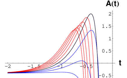
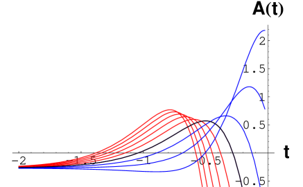
(a)                                                                       (b)

Figure 1: (a) $A(t)$ as a function of $t$ in Case [CC] with $k_{b}=-1$. The curve in black indicates the commutative case ($\theta=0$). The red curves correspond to the cases with $\theta=0.1,0.2,0.3,0.4,0.5$, according to the location of the peak from top to bottom. The blue curves correspond to the cases with $\theta=-0.1,-0.2,-0.3$, according to the location of the peak from top to bottom. (b) $A(t)$ as a function of $t$ in Case [CF]. The red curves correspond to the cases with $\theta=0.1,0.2,0.3,0.4,0.5$, according to the location of the peak from bottom to top. The blue curves correspond to the cases with $\theta=-0.1,-0.2,-0.3$, according to the location of the peak from bottom to top. For the other parameters for each fugure, see text.

We first consider Case [CC], with $k_{b}=-1$, $D=4$, $q=2$, $t_{0}=0$ and $P=2$. As already known, the model with $k_{b}=-1$, i.e., with the hyperbolic internal space, yields an accelerating universe TW ; Ohta2 . We show the values $A(t)=-S^{D-2}(t)\frac{d^{2}S^{2-D}(t)}{dt^{2}}$ versus $t$ for $\theta=-0.3\sim 0.5$ in FIG. 1 (a). The plot shows that acceleration is weakened for nonzero values of the noncommutativity parameter $\theta$. For $\theta>0$, we find that the acceleration period remains for a broad range of parameters. On the other hand, for $\theta<0$, the acceleration period disappears for sufficient large values of $|\theta|$. The same tendencies are found in Case [CL] with $\Lambda>0$ and Case [RP] with $p>1$. In general, the similar behavior of the scale factor is found in the case with $V>0$ and $\Sigma>0$.

Next, we consider Case [CF], with $f=1$, $D=4$, $q=2$, $t_{0}=0$ and $P=2$. The similar model with the flux and the dilaton field has been studied in the literature including Ref. CGG ; Roy . We show the values $A(t)=-S^{D-2}(t)\frac{d^{2}S^{2-D}(t)}{dt^{2}}$ versus $t$ for $\theta=-0.3\sim 0.5$ in FIG. 1 (b) in Case [CF]. The acceleration is strengthened for finite values of $|\theta|$, conversely to Case [CC]. In general, the similar behavior of the scale factor is found in the cases with $V>0$ and $\Sigma<0$.

To summarize, in the model described by the action with an exponential scalar potential (2) with $V>0$, the noncommutativity reduces the cosmic acceleration if $\alpha^{2}<\frac{D-1}{2(D-2)}$ while the noncommutativity enhances the acceleration if $\alpha^{2}>\frac{D-1}{2(D-2)}$.

V The quantum system

V.1 Wave function of the universe

In a commutative model, we can obtain the minisuperspace Wheeler–De Witt equation by replacing $\pi_{x}\rightarrow-i\frac{\partial}{\partial x}$ and $\pi_{y}\rightarrow-i\frac{\partial}{\partial y}$ in the Hamiltonian $H$ and regarding the Hamiltonian constraint as $H\Psi(x,y)=0$, where $\Psi(x,y)$ is the wave function of the universe Halliwell .

Deformation of the Wheeler-De Witt equation in our noncommtative case with the Hamiltonian $H_{\theta}$ can be performed by

$$X\rightarrow\hat{X}=x+i\frac{\theta-\rho}{2}\frac{\partial}{\partial y}\,,\quad Y\rightarrow\hat{Y}=y-i\frac{\theta+\rho}{2}\frac{\partial}{\partial x}\,,$$

$$\Pi_{X}\rightarrow\hat{\Pi}_{X}=-i\frac{\partial}{\partial x}\,,\quad\Pi_{Y}\rightarrow\hat{\Pi}_{Y}=-i\frac{\partial}{\partial y}\,.$$ (54)

These operators satisfy the relations

$$[\hat{X},\hat{\Pi}_{X}]=i\,,\quad[\hat{Y},\hat{\Pi}_{Y}]=i\,,\quad[\hat{X},\hat{Y}]=i\theta\,,$$ (55)

and other commutators vanish.

The corresponding Wheeler-De Witt equation is found to be

$$\frac{1}{2}\left\{\frac{\partial^{2}}{\partial x^{2}}-\frac{\partial^{2}}{\partial y^{2}}+U\exp\left[2\lambda\left(x+i\frac{\theta-\rho}{2}\frac{\partial}{\partial y}\right)\right]\right\}\Psi(x,y)=0\,.$$ (56)

The solution of the equation can be written as GOR ; ALNW

$$\Psi(x,y)=\int_{-\infty}^{\infty}d\nu\,{\cal A}_{\nu}\,\Psi_{\nu}(x,y)=\int_{-\infty}^{\infty}d\nu\,{\cal A}_{\nu}\,\psi_{\nu}(x)\,e^{i\nu(y-y_{0})}\,,$$ (57)

where

$$\psi_{\nu}(x)=c_{1}F_{i\nu/\lambda}(\sqrt{U}e^{\lambda[x-\nu(\theta-\rho)/2]}/\lambda)+c_{2}G_{i\nu/\lambda}(\sqrt{U}e^{\lambda[x-\nu(\theta-\rho)/2]}/\lambda)\,,\quad(U>0)$$ (58)

with

$$F_{\nu}(z)\equiv\frac{1}{2\cos(\nu\pi/2)}[J_{\nu}(z)+J_{-\nu}(z)]\,,\quad G_{\nu}(z)\equiv\frac{1}{2\sin(\nu\pi/2)}[J_{\nu}(z)-J_{-\nu}(z)]\,,$$ (59)

and

$$\psi_{\nu}(x)=c_{3}K_{i\nu/\lambda}(\sqrt{|U|}e^{\lambda[x-\nu(\theta-\rho)/2]}/\lambda)\,.\quad(U<0)$$ (60)

In the above expressions, ${\cal A}_{\nu}$ is the overall amplitude for $\nu$ and $c_{1},c_{2}$ and $c_{3}$ are normalization factors. $J_{\nu}(z)$ and $K_{\nu}(z)$ represent the Bessel function and the modified Bessel function of the second kind, respectively.

In the noncommutative case, we would like to consider $\Psi(X,Y)$ instead of $\Psi(x,y)$, i.e., the expression in the main noncommutative variables. In our model, the relation $\hat{\Pi}_{Y}\Psi_{\nu}=\nu\Psi_{\nu}$ holds. Moreover, if we take the parameter choice $\rho=-\theta$, we find that $Y$ equals $y$. Therefore, we can regard $X\sim x-\theta P$ approximately at this parameter choice, where $P$ is the most probable value of $\nu$ for the peaked wave packet.

The Gaussian wave packet has often been considered many times ALNW ; KN ; Kiefer1 ; Kiefer2 in a semiclassical analysis of quantum cosmology. For simplicity in calculations, we adopt here a rectangular form of the amplitude, which is finite in the width $\Gamma$ around the central value $\nu=P$, i.e.,

$${\cal A}_{\nu}=\Gamma^{-1/2}\quad(P-\Gamma/2<\nu<P+\Gamma/2)\,,\mbox{~{}and~{}}{\cal A}_{\nu}=0\quad(\nu<P-\Gamma/2,\,P+\Gamma/2<\nu)\,,$$ (61)

where $\Gamma$ is a constant. Fortunately, we will find that the dependence on noncommutativity has more influence than the choice of the shape of amplitude.

First, we consider the case with $U>0$ (58). We set the factors as ALNW

$$c_{1}=\sqrt{\frac{\nu/\lambda}{\tanh(\nu\pi/(2\lambda))}}\,,\quad c_{2}=0\,.$$ (62)

The choice that $c_{1}=0$ and $c_{2}\neq 0$ and the other general choices will lead to a similar result, because $F_{\nu}(e^{x})$ and $G_{\nu}(e^{x})$ have only the different phase shift in $x$ ALNW .

We show the density plot of the probability distribution $\varrho(X,Y)\equiv|\Psi(X,Y)|^{2}$ with the parameter $\rho=-\theta$ against $X\equiv x-\theta P$ and $Y=y$ in the case with $U>0$ in FIG. 2. Here, we consider Case [CC] with $k_{b}=-1$, $D=4$, $q=2$, $t_{0}=0$ and $P=2$ and set $\Gamma=5$. The figures correspond to the case with: (a) $\theta=0$, (b) $\theta=0.1$, (c) $\theta=-0.1$. The solid curves in figures shows the classical solutions (42).

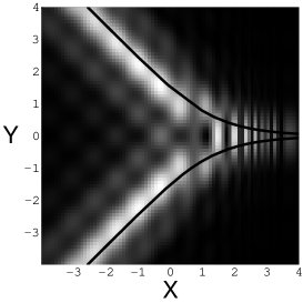
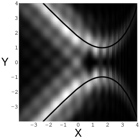
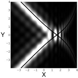
(a)                                         (b)                                         (c)

Figure 2: The probability distribution $\varrho\equiv|\Psi(X,Y)|^{2}$ in the case with $U>0$. The figures correspond to the case with: (a) $\theta=0$, (b) $\theta=0.1$, (c) $\theta=-0.1$. For the other parameters, see text.

Next, we consider the case with $U<0$ (60). We set the factors as

$$c_{3}=\sqrt{\frac{2(\nu/\lambda)\sinh(\pi\nu/\lambda)}{\pi}}\,.$$ (63)

We plot $\varrho=|\Psi(X,Y)|^{2}$ with the parameter $\rho=-\theta$ against $X=x-\theta P$ and $Y=y$ in the case with $U<0$ in FIG. 3. Here, we consider Case [CF] with $f=1$, $D=4$, $q=2$, $t_{0}=0$ and $P=2$ and set $\Gamma=5$. The figures correspond to the case with: (a) $\theta=0$, (b) $\theta=0.1$, (c) $\theta=-0.1$. The solid curves in figures shows the classical solutions (43).

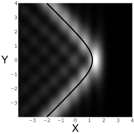
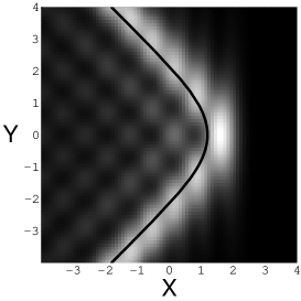
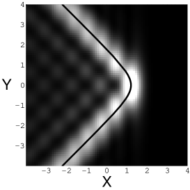
(a)                                         (b)                                         (c)

Figure 3: The probability distribution $\varrho\equiv|\Psi(X,Y)|^{2}$ in the case with $U<0$. The figures correspond to the case with: (a) $\theta=0$, (b) $\theta=0.1$, (c) $\theta=-0.1$. For the other parameters, see text.

In each case, one finds that the peak of the distribution function reproduces a classical trajectory well, even with the simplest rectangular form of amplitude adopted here.

The interpretation of the noncommutative variables, especially $X$ in the present case may not be accepted in general noncommutative dynamics, since the ‘expectation value’ $P$ for $\nu$ corresponds to a unique constant in our classical model.

V.2 Wigner function and deformation

In the previous subsection, we utilized the expectation value of $p_{y}\approx\nu$ to define the noncommutative variable $X$. In general, the noncommutative variable can be obtained from the linear combination of phase space variables, say, $x$ and $p_{y}$ in the two dimensional commutative system. Now, we propose another candidate of probability distribution by using the Wigner function Wigner ; WF and examine its validity by analysis with our soluble model. The Wigner function gives a (pseudo) probability distribution whose arguments are dynamical variables and their conjugate variables.

Generally speaking, the Wigner function Wigner ; WF is defined, in terms of a wave function $\phi(q)$, by

$$W(q,p)\equiv\frac{1}{2\pi}\int_{-\infty}^{\infty}du\,\phi^{*}\left(q-\frac{u}{2}\right)\phi\left(q+\frac{u}{2}\right)e^{-ipu}\,.$$ (64)

The Wigner function has beautiful properties, such as

$$\int_{-\infty}^{\infty}dp\,W(q,p)=\left|\phi\left(q\right)\right|^{2}\,,\quad\int_{-\infty}^{\infty}dq\,W(q,p)=|\tilde{\phi}\left(p\right)|^{2}\,,$$ (65)

where $\tilde{\phi}(p)$ is the Fourier transform of $\phi(q)$.

The application of the Wigner function has been considered already in quantum cosmologies with deformed phase spaces with slightly different motivations from ours CGT ; RJ . Our present aim is to construct the probability distribution whose arguments are noncommutative variables, say, $X$ and $Y$, from the Wigner function defined by the wave function of commutative variables $x$ and $y$.

We start with the Wigner distribution function constructed from the wave function $\Psi(x,y)$ (57), where we leave the variable $x$ untouched:

$$W(x,y,p_{y}) = \frac{1}{2\pi}\int_{-\infty}^{\infty}dv\,\Psi^{*}\left(x,y-\frac{v}{2}\right)\Psi\left(x,y+\frac{v}{2}\right)e^{-ip_{y}v}$$ (66)

$$= \frac{1}{2\pi}\int_{-\infty}^{\infty}d\nu^{\prime}\int_{-\infty}^{\infty}d\nu\,{\cal A}_{\nu^{\prime}}^{*}\psi^{*}_{\nu^{\prime}}(x){\cal A}_{\nu}\psi_{\nu}(x)e^{i(\nu-\nu^{\prime})(y-y_{0})}\int_{-\infty}^{\infty}dv\,e^{-i[p_{y}-(\nu^{\prime}+\nu)/2]v}$$

$$= \int_{-\infty}^{\infty}d\nu\,{\cal A}_{p_{y}-\nu/2}^{*}\psi^{*}_{p_{y}-\nu/2}(x){\cal A}_{p_{y}+\nu/2}\psi_{p_{y}+\nu/2}(x)e^{i\nu(y-y_{0})}\,.$$

Therefore, the Fourier transform between $y$ and $\nu$ is easily obtained as a simple form:

$$\tilde{W}(x,\nu,p_{y}) \equiv \frac{1}{2\pi}\int_{-\infty}^{\infty}dy\,W(x,y,p_{y})e^{-i\nu(y-y_{0})}$$ (67)

$$= {\cal A}_{p_{y}-\nu/2}^{*}\psi^{*}_{p_{y}-\nu/2}(x){\cal A}_{p_{y}+\nu/2}\psi_{p_{y}+\nu/2}(x)\,.$$

Now, we come to an idea that one may interpret $X=x-\theta p_{y}$ as in the relation (44) with $\rho=-\theta$. To this end, we define

$$X\equiv x-\theta p_{y}\,,\quad\tilde{X}\equiv\theta x+p_{y}\,,$$ (68)

and integrate out the extra variable $\tilde{X}$. Namely, we propose a (Fourier transformed) probability distribution

$$\tilde{\varrho}_{W}(X,\nu)\equiv\frac{1}{1+\theta^{2}}\int_{-\infty}^{\infty}d\tilde{X}\,\tilde{W}(x(X,\tilde{X}),\nu,p_{y}(X,\tilde{X}))\,,$$ (69)

where

$$x(X,\tilde{X})=\frac{1}{1+\theta^{2}}(X+\theta\tilde{X})\,,\quad p_{y}(X,\tilde{X})=\frac{1}{1+\theta^{2}}(\tilde{X}-\theta X)\,.$$ (70)

To compare the new probability distribution with that considered in the last section, we consider the Fourier transform of $\rho(X,Y)$:

$$\tilde{\cal\varrho}(X,\nu) = \frac{1}{2\pi}\int_{-\infty}^{\infty}dy\int_{-\infty}^{\infty}d\nu^{\prime\prime}\int_{-\infty}^{\infty}d\nu^{\prime}\,{\cal A}_{\nu^{\prime\prime}}^{*}\psi^{*}_{\nu^{\prime\prime}}(X+\theta P){\cal A}_{\nu^{\prime}}\psi_{\nu^{\prime}}(X+\theta P)e^{i(\nu^{\prime}-\nu^{\prime\prime})(y-y_{0})}\,e^{-i\nu(y-y_{0})}$$ (71)

$$= \int_{-\infty}^{\infty}d\nu^{\prime}\,{\cal A}_{\nu^{\prime}-\nu/2}^{*}\psi^{*}_{\nu^{\prime}-\nu/2}(X+\theta P){\cal A}_{\nu^{\prime}+\nu/2}\psi_{\nu^{\prime}+\nu/2}(X+\theta P)\,.$$

These expressions show the fact that $\tilde{\cal\varrho}_{W}(X,\nu)$ can be very close to $\tilde{\cal\varrho}(X,\nu)$ if the amplitude ${\cal A}_{\nu}$ has the compact form of which central value is located at $\nu\sim P$. One can also find that $\tilde{\cal\varrho}_{W}(X,\nu)$=$\tilde{\cal\varrho}(X,\nu)$ exactly in the commutative case with $\theta=0$.

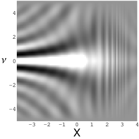
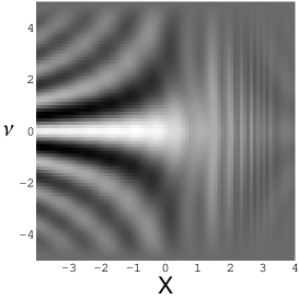
(a)                                         (b)                                         (c)

Figure 4: The new Fourier transformed probability distribution $\tilde{\varrho}_{W}(X,\nu)$ in the case with $U>0$. The figures correspond to the case with: (a) $\theta=0$, (b) $\theta=0.1$, (c) $\theta=-0.1$.

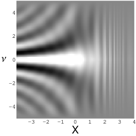
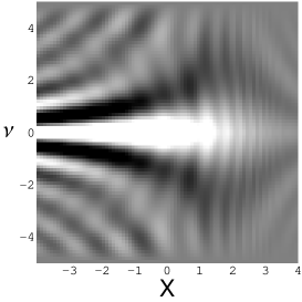
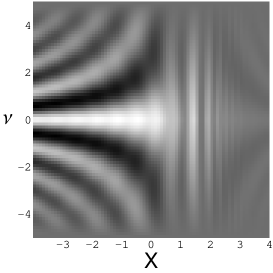
(a)                                         (b)                                         (c)

Figure 5: The Fourier transform of the probability distribution defined in the previous section, $\tilde{\varrho}(X,\nu)$ in the case with $U>0$ for comparison. The figures correspond to the case with: (a) $\theta=0$, (b) $\theta=0.1$, (c) $\theta=-0.1$.

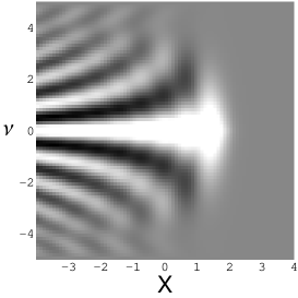
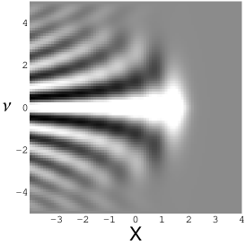
(a)                                         (b)                                         (c)

Figure 6: The new Fourier transformed probability distribution $\tilde{\varrho}_{W}(X,\nu)$ in the case with $U<0$. The figures correspond to the case with: (a) $\theta=0$, (b) $\theta=0.1$, (c) $\theta=-0.1$.

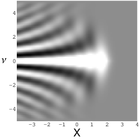
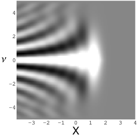
(a)                                         (b)                                         (c)

Figure 7: The Fourier transform of the probability distribution defined in the previous section, $\tilde{\varrho}(X,\nu)$ in the case with $U<0$ for comparison. The figures correspond to the case with: (a) $\theta=0$, (b) $\theta=0.1$, (c) $\theta=-0.1$.

The numerical calculations for the probability distributions are shown in FIG. 4, FIG. 5, FIG. 6, and FIG. 7. The case with $U>0$ is shown in FIG. 4 and FIG. 5. FIG. 4 represents $\tilde{\varrho}_{W}(X,Y)$ while FIG. 5 represents $\tilde{\varrho}(X,Y)$ which is the Fourier transform of the distribution $\varrho(X,Y)$ considered in the previous section. In the figures, the noncommutative parameter is set to: (a) $\theta=0$, (b) $\theta=0.1$, and (c) $\theta=-0.1$. One can hardly find notable differences between FIG. 4 and FIG. 5. Similarly, the case with $U<0$ is shown in FIG. 6 and FIG. 7. Any remarkable difference cannot be found also in this case.

Consequently, it is safely to say that the newly defined distribution function $\tilde{\varrho}_{W}(X,Y)$ is valid for describing the present model. Note that our present model and analysis may be very specific; we have only studied quantum cosmologies in terms of wave packets, which have rather semiclassical properties and is easy to treat. The study of the probability distribution derived from the Wigner function in terms of generic wave functions will be expected in future work. Nonetheless, the verification of the validity through the exact analytic solutions in the present work is the first essential step to study the noncommutative quantum cosmology with noncommutative variables.

VI discussion and outlook

In this paper, a noncommutative deformation of the minisuperspace variables is studied by means of an integrable model. Its analytical solutions are obtained in classical and quantum cosmology.

It has been already known that the $D$-dimensional model with an exponential scalar potential $\frac{V}{2}e^{2\alpha\phi}$, which is related to higher-dimensional/higher-derivative theories, gives rise to an accelerating universe. We find that the noncommutativity suppresses acceleration if the coupling $\alpha$ is small whereas it enhances acceleration if the coupling $\alpha$ is large, provided that $V>0$. The critical value is given by $\alpha^{2}={\frac{D-1}{2(D-2)}}$ in our model.

The different behaviors, which depend on the sign of $U$, should be thoroughly investigated both in classical and quantum perspectives, since interesting features in the Liouville quantum mechanics with a negative potential have been reported KT . This issue is left for a future work.

We have managed to interpret the probability distribution in noncommutative quantum cosmology. We first showed that the peak of the wave packet reproduces the classical trajectory by using exact solutions with an interpretation of the noncommutative variables in the present model. Next, we proposed a new probability distribution in noncommutative quantum cosmology constructed from the Wigner function. Its validity in the present solvable model is confirmed numerically.

In general, the Wigner function is not positive-definite, as is well-known. Although our study focusing on wave packets is not suffering from the problem of ‘negative probability’, we should treat carefully the problem with general settings and we have to search for a possible solution to the problem.

In future study, we will investigate general noncommutative cosmology by using the probability distribution function provided in this paper. Also, general deformations of minisuperspace variables should be studied further. The model with a phantom scalar field phantom ; DKS ; ALNW and/or a phantom gauge field KS may also be worth studying in the context of noncommutative cosmology.

References

- (1) M. R. Douglas and N. A. Nekrasov, Rev. Mod. Phys. 73 (2001) 977.
- (2) R. J. Szabo, Phys. Rep. 378 (2003) 207.
- (3) H. García-Compeán, O. Obregón and C. Ramírez, Phys. Rev. Lett. 88 (2002) 161301.
- (4) G. D. Barbosa and N. Pinto-Neto, Phys. Rev. D70 (2004) 103512.
- (5) L. O. Pimentel and C. Mora, Gen. Rel. Grav. 37 (2005) 817.
- (6) L. O. Pimentel and O. Obregón, Gen. Rel. Grav. 38 (2006) 553.
- (7) M. Aguero, J. A. S. Aguilar, C. Ortiz, M. Sabido and J. Socorro, Int. J. Theor. Phys. 46 (2007) 2928.
- (8) W. Guzmán, M. Sabido and J. Socorro, Phys. Rev. D76 (2007) 087302.
- (9) W. Guzmán, M. Sabido and J. Socorro, Rev. Mex. Fís. 53 suppl. 4 (2007) 94.
- (10) W. Guzmán, M. Sabido and J. Socorro, AIP Conf. Proc. 1318 (2010) 209.
- (11) E. Mena, O. Obregón and M. Sabido, Rev. Mex. Fís. 53 suppl. 4 (2007) 118.
- (12) E. Mena, O. Obregón and M. Sabido, Int. J. Mod. Phys. D18 (2009) 95.
- (13) C. Ortiz, E. Mena, M. Sabido and J. Socorro, Int. J. Theor. Phys. 47 (2008) 1240.
- (14) J. Socorro, L. O. Pimentel, C. Ortiz and M. Aguero, Int. J. Theor. Phys. 48 (2009) 3567.
- (15) C. Bastos, O. Bertolami, N. C. Dias and J. N. Prata, Phys. Rev. D78 (2008) 023516.
- (16) C. Bastos, O. Bertolami, N. C. Dias and J. N. Prata, J. Phys. Conf. Ser. 174 (2009) 012053.
- (17) C. Bastos, O. Bertolami, N. Dias and J. N. Prata, Int. J. Mod. Phys. A24 (2009) 2741.
- (18) M. Maceda, A. Macías and L. O. Pimentel, Phys. Rev. D78 (2008) 064041.
- (19) O. Obregón and I. Quiros, Phys. Rev. D84 (2011) 044005.
- (20) L. Amendra and S. Tsujikawa, “Dark energy: theory and observations”, (Cambridge University Press, New York, 2010).
- (21) E. J. Copeland, M. Sami and S. Tsujikawa, Int. J. Mod. Phys. D15 (2006) 1753.
- (22) A. D. Linde, “Particle physics and inflationary cosmology”, Contemporary Concepts in Physics 5, (Harwood Academic Pub., Philadelphia, 1990).
- (23) P. K. Townsend and M. N. R. Wohlfarth, Phys. Rev. Lett. 91 (2003) 061302.
- (24) N. Ohta, Phys. Rev. Lett. 91 (2003) 061303.
- (25) C.-M. Chen, D. V. Gal’tsov and M. Gutperle, Phys. Rev. D66 (2002) 024043.
- (26) S. Roy, Phys. Lett. B567 (2003) 322.
- (27) I. P. Neupane, Class. Quant. Grav. 21 (2004) 4387.
- (28) J. G. Russo, Phys. Lett. B600 (2004) 185.
- (29) S. Mignemi and N. Pintus, Gen. Rel. Grav. 47 (2015) 51.
- (30) N. Pintus and S. Mignemi, J. Phys. Conf. Series 956 (2018) 012022.
- (31) A. A. Andrianov, C. Lan, O. O. Novikov and Y.-F. Wang, Eur. J. Phys. C78 (2018) 786.
- (32) N. Kan, M. Kuniyasu, K. Shiraishi and K. Takimoto, Phys. Rev. D98 (2018) 044054.
- (33) N. Kan, K. Shiraishi and M. Yashiki, Gen. Rel. Grav. 51 (2019) 90.
- (34) E. Wigner, Phys. Rev. 40 (1932) 749.
- (35) J. Weinbub and D. K. Ferry, App. Phys. Rev. 5 (2018) 041104.
- (36) S. J. Poletti and D. L. Wiltshire, Phys. Rev. D50 (1994) 7260.
- (37) S. Mignemi, Int. J. Mod. Phys. 28 (2013) 1350080.
- (38) C. Simeone, “Deparametrization and path integral quantization of cosmological models”, (World Scientific Lecture Notes in Physics–Vol. 69, World Scientific, Singapore, 2001).
- (39) J. W. York, Phys. Rev. Lett. 28 (1972) 1082.
- (40) G. W. Gibbons and S. W. Hawking, Phys. Rev. D15 (1972) 2752.
- (41) A. E. F. Djemai, Int. J. Theor. Phys. 43 (2004) 299.
- (42) J. J. Halliwell, “Introductory Lectures on Quantum Cosmology”, in Proceedings of the Jerusalem Winter School on Quantum Cosmology and Baby Universe (edited by T. Piran, World Scientific, Singapore, 1991).
- (43) Y. Kazama and R. Nakayama, Phys. Rev. D32 (1985) 2500.
- (44) C. Kiefer, Phys. Rev. D38 (1988) 1761.
- (45) C. Kiefer, Nucl. Phys. B341 (1990) 273.
- (46) R. Cordero, H. García-Compeán and F. J. Turrubiates, Phys. Rev. D83 (2011) 125030.
- (47) M. Rashki and S. Jalalzadeh, Gen. Rel. Grav. 49 (2017) 14.
- (48) H. Kobayashi and I. Tsutsui, Nucl. Phys. B472 (1996) 409.
- (49) R. R. Caldwell, Phys. Lett. B545 (2002) 23.
- (50) M. P. Dabrowski, C. Kiefer and B. Sandhöfer, Phys. Rev. D74 (2006) 044022.
- (51) D. E. Kaplan and R. Sundrum, JHEP 0607 (2006) 042.