The galaxy luminosity function in the LAMOST Complete Spectroscopic Survey of Pointing Area at the Southern Galactic Cap

Abstract

We present optical luminosity functions (LFs) of galaxies in the ${}^{0.1}g$, ${}^{0.1}r$, and ${}^{0.1}i$ bands, calculated using data in $\sim 40$ $deg^{2}$ sky area of LAMOST Complete Spectroscopic Survey of Pointing Area (LaCoSSPAr) in Southern Galactic Cap. Redshifts for galaxies brighter $r=18.1$ were obtained mainly with LAMOST. In each band, LFs derived using both parametric and non-parametric maximum likelihood methods agree well with each other. In the ${}^{0.1}r$ band, our fitting parameters of the Schechter function are $\phi_{*}=(1.65\pm 0.36)\times 10^{-2}h^{3}Mpc^{-3}$, $M_{*}=-20.69\pm 0.06$ mag, and $\alpha=-1.12\pm 0.08$, in agreements with previous studies. Separate LFs are also derived for emission line galaxies and absorption line galaxies, respectively. The LFs of absorption line galaxies show a dip at ${}^{0.1}r\sim 18.5$ and can be well fitted by a double-Gaussian function, suggesting a bi-modality in passive galaxies.

1 Introduction

Luminosity is one of the most basic properties of galaxies. Studies of galaxy luminosity functions (LFs) give direct statistical estimates for the space density of galaxies with respect to their luminosities, and provide important information about the galaxy formation and evolution.

In recent years, many large spectroscopic surveys have been conducted to investigate the nearby universe. Among them, the Center for Astrophysics (CfA) Survey (Huchra et al. [1983]), the Two-Degree Field (2dF) Galaxy Redshift Survey (Lewis et al. [2002]), the Sloan Digital Sky Survey (SDSS; York et al. [2000]), and the Galaxy And Mass Assembly (GAMA) redshift survey (Driver et al. [2009]; Baldry et al. [2010]), etc., were all very successful and gave us a better understanding of the universe. Thanks to these surveys, many investigations of galaxy LFs have been done, providing important observing constraints on theories of galaxy formation and evolution.

Blanton et al. ([2001]) calculated the galaxy LFs in SDSS $ugriz$ bands using SDSS commissioning data and discussed the dependence of luminosity on surface brightness, color and morphology. Blanton et al. ([2003]) fitted the LFs using two parameters, Q and P, to study effects of luminosity and density evolution, respectively. Montero-Dorta & Prada ([2009]) calculated the luminosity function with a sample selected from SDSS DR6 (Adelman-McCarthy et al. [2008]), and found a remarkable excess at the bright end of the ${}^{0.1}u$ band LF. Loveday et al. ([2012]) focused on the evolution of the LFs in a redshift range of $0.002<z<0.5$ and pointed out different evolution features between blue galaxies and red galaxies based on GAMA core data release (Driver et al. [2011]).

At higher redshift ($z>0.5$), Willmer et al. ([2006]) constructed $B$-band LFs of red and blue galaxies in different redshift slices from $z\sim 0.2$ to $z\sim 1.2$ based on the Deep Evolutionary Exploratory Probe 2 redshift survey (DEEP2; Davis et al. [2003]), and found a more significant luminosity evolution for blue galaxies while for red galaxies a more significant density evolution. Montero-Dorta et al. ([2016]) used the Baryon Oscillation Spectroscopic Survey (BOSS; Dawson et al. [2013]) high redshift sample, and computed the high mass end of the SDSS ${}^{0.55}i$ band luminosity functions of red sequence galaxies at redshift $z\sim 0.55$, they suggested that these red sequence galaxies formed at redshift $z=1.5-3$. L$\acute{o}$pez-Sanjuan et al. ([2017]) studied the B-band luminosity functions for star-forming and quiescent galaxies based on ALHAMBRA (Advanced, Large, Homogeneous Area, Mediam-Band Redshift Astronomical) survey (Moles et al. [2008]), and provided a distinct understanding of the evolution of B-band luminosity function and luminosity density for different types of galaxies since $z\sim 1$.

The Large Sky Area Multi-Object Fiber Spectroscopic Telescope (LAMOST) is a Wang-Su reflecting Schmidt telescope (Wang et al. [1996]; Su & Cui [2004]; Cui et al. [2012]; Zhao et al. [2012]) located in Xinglong Station of National Astronomical Observatory, Chinese Academy of Sciences (NAOC). Thanks to its $\sim 20$ $deg^{2}$ field of view (FOV) and 4000 fibers, LAMOST can spectroscopically observe more than 3000 scientific targets simultaneously (nearly 5 times more than SDSS), making it efficient to obtain spectra of celestial objects. LAMOST ExtraGAlactic Survey (LEGAS), an important part of LAMOST scientific survey, aims to cover $\sim 8000deg^{2}$ of the Northern Galactic Cap (NGC) and $\sim 3500deg^{2}$ of the Southern Galactic Cap (SGC) and take hundreds of thousands of spectra for extra-galactic objects with redshifts $z<0.3$ in five years (Yang et al. [2018]). When finishing its extra-galactic survey, LAMOST will provide a catalog, covering large sky area ($\sim 11500deg^{2}$ in total) and containing millions of spectroscopic information of galaxies.

This work is based on LAMOST Complete Spectroscopic Survey of Pointing Area (LaCoSSPAr), an early project of LEGAS. The LaCoSSPAr is a LAMOST key project aiming at observing all sources (galactic and extra-galactic) with a magnitude limit of $14.0<r<18.1$ in selected two 20 $degree^{2}$ regions in SGC, where the faint magnitude limit is 0.1 mag deeper than LAMOST designed and 0.33 mag deeper than that of SDSS legacy survey. This survey is designed to investigate the completeness and selection effects in the wider LEGAS survey (Yang et al. [2018]). By using the spectra observed by LAMOST and cross-matching with data of other photometric surveys, the galaxy LFs can be investigated in specific bands. Our fields locate in the SGC, where the footprint covered by the SDSS is small. Meanwhile, thanks to the high galactic latitude, our galaxy sample suffers less from the effects of Galactic extinction.

In this paper, we use the galaxy redshift sample based on LaCoSSPAr, which is the most complete sample in LEGAS up to now, and combine with SDSS Petrosian magnitudes, to estimate the galaxy LFs in SDSS ${}^{0.1}g$, ${}^{0.1}r$, ${}^{0.1}i$ bands. Our sample has a fainter limiting magnitude than SDSS and our goal is to achieve a better understanding about the faint end of galaxy LFs. In section 2, we give an introduction to LAMOST data and data reduction, and describe our sample selection and correction for the incompleteness. In section 3, we introduce the methods used to estimate the galaxy LFs. And in section 4, we present the results of the LFs and discussion. A summary is presented in section 5. Throughout this paper, we adopt a Friedmann-Robertson-Walker cosmological world model with constants of $\Omega_{m}=0.3$,$\Omega_{\Lambda}=0.7$ and $H_{0}=70$ $kms^{-1}Mpc^{-1}$.

2 Sample

2.1 LaCoSSPAr, data and data reduction

The LaCoSSPAr surveys two $\sim 20$ $degree^{2}$ regions in SGC with limiting magnitude of $r=18.1$ mag. Originally, the plan was to select a higher density region and a lower density region to test possible environmental effects. The high density field (Field B: $R.A.=21.53^{\circ}$, $Dec.=-2.20^{\circ}$) is selected to cover a large Abell rich cluster (Abell et al. [1989]), and the low density field (Field A: $R.A.=37.88^{\circ}$, $Dec.=3.44^{\circ}$) is selected in a blank region near Field B (as shown in Figure 1 in Yang et al. [2018]). However, it was found later that Field A (low density field) actually contains 11 faint Abell and Zwicky clusters and therefore may not represent low density regions. The effects of the field selection will be discussed in Section 4.

The input catalog for targets of LaCoSSPAr survey were selected from the Data Release 9 (DR9; Ahn et al. [2012]) of the SDSS PhotoPrimary database, using the criteria of $14.0<r<18.1$ and type =‘Galaxy’. Sources (936) were excluded when they are in the following special regions that are not observed by LAMOST: (1) in the LAMOST five guide CCDs fields, (2) within 10" from bright stars, and (3) in dense regions. The final LaCoSSPAr target catalog contains 5623 sources, of which 5442 (96.8%) were observed successfully, and 181 (3.2%) failed mainly due to bad fibers.

The raw data of successful observations were first reduced by the LAMOST 2D and 1D pipelines (Luo et al. [2012]), which include bias subtraction, flat-fielding through twilight exposures, cosmic-ray removal, spectrum extraction, wavelength calibration, sky subtraction and exposure coaddition. However, for many spectra with relatively low SNR the pipeline does not work well. Low SNR makes it hard to recognize diagnostic lines. Also, bad sky line subtraction often introduces fake lines that affect significantly the redshift measurement. Consequently, only about a third of total observed galaxies obtained redshifts from the pipeline. In order to achieve better redshift detection rate, additional data processing of the 1D spectrum is carried out using our own software (Yang et al. [2018]). Briefly speaking, in order to improve the results of sky line subtraction, in the residual spectrum we replaced all $>3\sigma$ points around each skyline ($\pm 15\AA$) by the values of continuum fitting. After this, we inspected each spectrum by eyes (by at least two individuals) and re-measured the redshift by identifying emission lines and absorption lines. These new steps improved significantly the success rate of redshift detection (Bai et al. [2017]). Redshifts of 3098 sources were detected, corresponding to a detection rate of 55%. They have a median redshift of $\bar{z}=0.104$ and typical uncertainty of $\sigma_{z}/(1+z)<0.001$.

2.2 Parent Sample and Redshift Completeness

The parent sample for the LF calculations is based on the LaCoSSPAr target catalog (see Section 2.1). Actually, many sources in that catalog are stars or fake targets identified mistakenly as galaxies by SDSS. In order to exclude them, we inspected the images of all sources visually on the SDSS navigator tool and discarded those showing obvious characteristics of a star, or no show at all (fake sources). Furthermore, among the 3098 sources with LAMOST redshifts, 60 were found to be Galactic sources with z=0 and therefore were excluded. Finally, our parent sample contains 5531 galaxies, of which 3038 having redshifts from LAMOST. In addition, 457 galaxies in the sample have SDSS redshifts but no LAMOST redshifts. Altogether, 3495 galaxies in our sample have measured redshifts, corresponding to a redshift completeness of 63%. For galaxies brighter than the magnitude limit of SDSS spectroscopic survey, r=17.77 mag, the redshift completeness of the sample is 69% (2592/3749).

In Figure 1, the magnitude distribution of galaxies in the parent sample is presented. For each galaxy, the Galactic extinction was corrected using the dust maps of Schlegel, Finkbeiner & Davis ([1998]). Upper panel shows histograms of magnitudes in $gri$ bands for all visually-examined photometric galaxies. We use different colors to represent galaxies with redshifts from LaCoSSPAr (red), galaxies with redshifts from SDSS (orange) and galaxies having no redshifts (blue) in each bin. Lower panel gives the fraction for different classes within each magnitude bin. The black dashed lines mark the magnitude limits of corresponding subsamples used in the calculation of individual LFs. Beyond these limits, the completeness (i.e. the ratio between galaxies with redshifts and galaxies identified photometrically) drops rapidly below 50%. Figure 1 shows that the completeness of faint galaxies is better than that of bright galaxies. This counter-intuitive result deserves some explanation. It appears that the success of redshift detection depends sensitively on how accurately the fiber position coincides with the target position. Because targets fainter than $r=16$ were observed with longer integration times and more repeats (Yang et al. [2018]), they are more resilient against the effect of bad fiber position, and therefore have better detection rates.

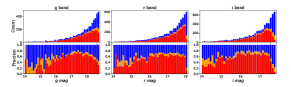
Figure 1: Upper panel: the histogram of Petrosian magnitude in each band for all galaxies in the parent sample. Different colors represent for galaxies with redshifts from LaCoSSPAr (red), galaxies having no LaCoSSPAr redshifts but having redshifts from SDSS (orange) and galaxies having no redshifts (blue). Lower panel: the fraction for different classes within each magnitude bin. The black dashed lines show the upper magnitude limit of subsample.

We checked the dependence of LaCoSSPAr redshift incompleteness on redshift itself by comparing with the SDSS spectroscopic sample. Given the magnitude limit of SDSS spectroscopic main galaxy sample, we plot in Figure 3 sky positions of all photometric galaxies (blue dots) and galaxies with SDSS redshifts (red dots), both brighter than $r=17.6$, in our two fields. The Stripe 82 of SDSS Legacy Survey (Abazajian et al. [2009]) overlaps with our survey, resulting in a higher SDSS redshift coverage between $-1.25^{\circ}<Dec.<1.25^{\circ}$, as presented in Figure 3. In order to construct a complete comparison sample, we divided our two fields into many grid cells and calculated the ratio between galaxies having SDSS redshifts and photometric galaxies for each cell. In Figure 3, we present the completeness map of SDSS survey in our two fields. The complete comparison sample (here after ‘sample C’) includes all galaxies located within cells that are $100\%$ complete and with $-1.25^{\circ}<Dec.<1.25^{\circ}$. It contains 120 galaxies.

A plot of the redshift dependence of the completeness is presented in Figure 4. In the upper panel, histograms of distributions of SDSS redshifts (blue bars) and LoCaSSPAr redshifts (orange bars) are plotted for sample C. The bin size has been adjusted to ensure roughly equal number of galaxies in each bin. The completeness and error are plotted in the lower panel. It appears that, for galaxies with $r<17.6$, the redshift completeness of LaCoSSPAr has two different levels for $z<\sim 0.08$ and $z>\sim 0.08$: $\sim 0.4$ for low redshift range and $\sim 0.7$ for high redshift range. In Figure 5, we divided the 120 galaxies in ‘sample C’ into a $z>0.08$ subsample and a $z<0.08$ subsample. Galaxies in the high redshift subsample are all with $r>16.0$ mag, so they have higher completeness. In the low redshift subsample, galaxies cover a large magnitude range from 14.4 mag to 17.6 mag. Among them, bright galaxies have lower completeness while faint galaxies still have relative higher completeness. It appears that the difference between redshift incompleteness in two redshift ranges is caused by the different incompleteness between bright and faint galaxies, as shown in Figure 1.

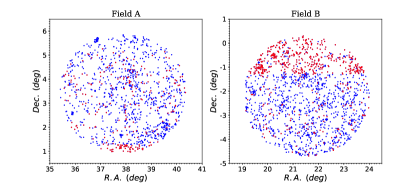
Figure 2: Spatial distribution for photometric galaxies (blue dots) and galaxies having SDSS redshifts (red dots) with $r<17.6$.

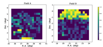
Figure 3: The completeness map for SDSS survey in our two fields. Color bar represents the ratio between galaxies having SDSS redshifts and photometric galaxies for each cell.

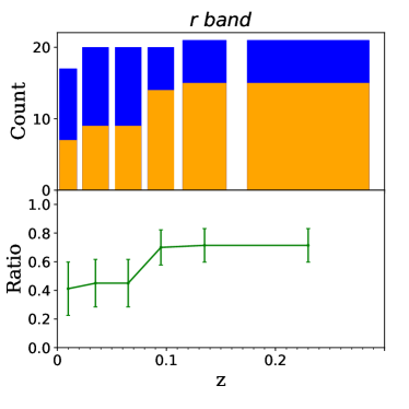
Figure 4: Relationship between redshift completeness of LaCoSSPAr and galaxy redshift. Upper panel: the histograms of redshift distribution. The blue bars and orange bars represent counts of redshifts from SDSS survey and from LaCoSSPAr, respectively. We only use the $100\%$ complete cells within $-1.25^{\circ}<Dec.<1.25^{\circ}$ in Figure 3 to calculate the galaxy numbers. The bin size are set to ensure roughly equal numbers of galaxies for blue bars in each bin. Lower panel: green dots show the ratio of number count of galaxies with LaCoSSPAr redshifts to number count of galaxies with SDSS redshifts in each bin in the upper panel.

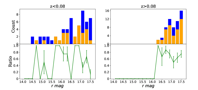
Figure 5: Upper panel: the histograms of Petrosian magnitude in r band for galaxies in ‘sample C’ (blue bars) and galaxies only with redshifts from LaCoSSPAr in ‘sample C’ (orange bars). These galaxies are divided into $z<0.08$ and $z>0.08$ panels. Lower panel: the ratio of counts in orange bars to counts in blue bars.

2.3 Samples for LFs in different bands

Samples for LFs in different bands were constructed by applying corresponding redshift limits and apparent magnitude limits to the parent sample. The lower magnitude limits were set to be 14.0 mag in all bands. The upper magnitude limit in $r$ band was set to be the same with that of LaCoSSPAr, $r<18.1$ mag. In other bands, we chose the upper limit at the magnitude where the redshift completeness falls rapidly (Figure 1). As for the redshift limits, we chose the upper redshift limits at where 98 percent of galaxies are included in the sample to avoid large noise in the determination of the normalization at high redshift. And the lower redshift limits are the same with that in Blanton et al. ([2001]), which can reduce the effect of galaxy peculiar velocities when calculating galaxy luminosity distance.

The lower and upper limits of redshift and magnitude along with the number of galaxies for the samples are listed in Table 1. In this work, we did not include the $u$, $z$ bands because of their relative large photometric uncertainties.

Table 1: Magnitude and redshift limits and galaxy counts of samples for LFs in different bands.

Band	Magnitude limits	Redshift limits	No. of Galaxies
$g$	$14.0<m<18.7$	$0.016<z<0.23$	2718
$r$	$14.0<m<18.1$	$0.016<z<0.27$	3412
$i$	$14.0<m<17.6$	$0.016<z<0.275$	3235

3 Luminosity functions

We used KCORRECT v4_3 (Blanton et al. [2007]) code to estimate the K-corrections for SDSS magnitudes. In order to compare with LFs in previous works based on SDSS data, we adopted ‘blueshift = 0.1’ when using this code, and obtained absolute magnitudes in z=0.1 blushifted bandpasses.

In LF calculations, we exploited two methods based on maximum likelihood approach. One is the parametric maximum likelihood method introduced by Sandage, Tammann & Yahil ([1979], the so called STY method). It is based on the probability for a galaxy of redshift $z_{i}$ and absolute magnitude $M_{i}$ to be included in a magnitude-limited sample:

$$p_{i}=\frac{\phi(M_{i})}{\int_{max[M_{min}(z_{i}),M_{1}]}^{min[M_{max}(z_{i}),M_{2}]}\phi(M)dM}$$ (1)

where $M_{min}(z_{i})$ and $M_{max}(z_{i})$ are the minimum and maximum absolute magnitudes a galaxy at redshift $z_{i}$ can have in order to be included in the sample, $M_{1}$ and $M_{2}$ are the absolute magnitude limit of the sample. In order to correct for the incompleteness, the following correcting factor $Fac_{n}(mag_{bin})$ is defined for every galaxy in each bin,

$$Fac_{n}(mag_{bin})=\frac{1}{Fraction_{red}(mag_{bin})+Fraction_{orange}(mag_{bin})}$$ (2)

Here $Fraction_{red}$ and $Fraction_{orange}$ correspond to red bars and orange bars presented in Figure 1. We assumed that the incompleteness depends only on the apparent magnitude. A Schechter function (Schechter [1976]) for $\phi(M)$ was adopted when maximizing the log-likelihood function $ln\mathcal{L}$,

$$\phi(M)=0.4ln(10)\phi_{*}10^{-0.4(M-M_{*})(\alpha+1)}exp(-10^{-0.4(M-M_{*})})$$ (3)

$$ln\mathcal{L}=\sum_{i}^{N_{gal}}{Fac_{i}lnp_{i}}$$ (4)

The other method, the Stepwise Maximum Likelihood Method (SWML), is a non-parametric method described by Efstathiou, Ellis & Peterson ([1988]). This method does not depend on any assumption on the particular form of an LF. The sample is divided into $N_{bin}$ bins according to the absolute magnitude, and the LF can be calculated as:

$$\phi(M)=\phi_{i},M_{i}-\Delta/2<M<M_{i}+\Delta/2,i=1,2,...,N_{bin}$$ (5)

where $\phi_{i}$ is the value of the LF in each bin, which can be derived iteratively by maximizing a log-likelihood function similar to that in Eq. (4).

For either method, we used the minimum variance estimator (Davis & Huchra ([1982]) to calculate independently the normalization constant $\bar{n}$ of each LF. $\bar{n}$ represents the number density of galaxies, and it can be expressed as:

$$\phi(M)=\bar{n}\phi^{*}(M)$$ (6)

where $\phi^{*}(M)$ is the unit-normalized luminosity function.

We did not carry out the correction for cosmic evolutionary effects because it may introduce significant uncertainties due to our relatively small sample size and large number of parameters involved in the calculation (Blanton et al. [2003]).

In the calculation of errors of the STY LFs, we used the jackknife re-sampling method which has been used in many previous work (Blanton et al. [2003]; Loveday et al. [2012]). We divided our total region into 8 sub-regions of approximately equal area, each time omitting 1 region in the calculation, and got a set of parameters $x^{k}=\{\alpha,M_{*},\bar{n}\}$. The statistical variance of the fitting parameter $x^{k}=\{\alpha,M_{*},\bar{n}\}$ can be written as

$$var(x^{k})=\frac{N-1}{N}\sum_{n=1}^{N}(x_{n}^{k}-\bar{x}^{k})^{2}$$ (7)

where N=8 is the number of jackknife regions and $\bar{x}^{k}$ is the mean of the parameter $x_{n}^{k}$ fitted while excluding region i. It should be pointed out that, for large samples covering widely separated sky areas (e.g. Blanton et al. [2003]), Jackknife method can include uncertainties due to large-scale structure across the survey, namely the cosmic variance. However, due to relatively small area of our survey, this does not apply to our results. Therefore, while the uncertainties of parameters ($\alpha$, $M_{*}$) in our work may be underestimated, the cosmic variance is added to the error of $\bar{n}$. It is estimated according to (Peebles et al. [1980]; Somerville et al. [2004]; Xu et al. [2012])

$$\sigma^{2}_{cv}=J_{2}(\gamma)\times(r_{0}/r_{sample})^{\gamma}$$ (8)

where $r_{0}=5.59h^{-1}Mpc$ and $\gamma=1.84$ (Zehavi et al. [2005]) are parameters in the two point correlation function, $r_{sample}$ represents the radius of sample volume, and $J_{2}$ is

$$J_{2}(\gamma)=\frac{72}{(3-\gamma)\times(4-\gamma)\times(6-\gamma)\times 2^{\gamma}}.$$ (9)

In ${}^{0.1}r$ band, the cosmic variance contributes $\sim 63.3\%$ of the error of $\bar{n}$.

For SWML LFs, the errors of $\phi_{i}$ were calculated using inversion of the information matrix as described in Efstathiou, Ellis & Peterson ([1988]).

In every band, we also calculated the luminosity density using parameters of corresponding STY LF:

$$j=\int_{0}^{\infty}dLL\phi(L)=\phi_{*}L_{*}\Gamma(\alpha+2).$$ (10)

4 The results and discussion

4.1 LFs and luminosity densities

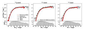
Figure 6: Upper panel: the LFs of LaCoSSPAr in SDSS ${}^{0.1}g,^{0.1}r,^{0.1}i$ bands. The black dots are the SWML LFs with error bars and black lines are the results of best Schechter function fit by using STY method. The red thick curves show the LFs of Blanton et al. ([2003]) along with its error region, and red lines are the best-fitting Schechter functions, both are under a simple evolution assumption. LFs of Field A and Field B are also plotted as squares and triangles, respectively. In r-band panel, we overplot the dotted line shown in Fig.15 in Blanton et al. ([2003]), which represent the best-fit Schechter function based on a sample of $\sim$ 10,000 galaxies, taking no account for the effect of evolution. Lower panel: histograms of the number of galaxies in each bin for SDSS ${}^{0.1}g,^{0.1}r,^{0.1}i$ bands.

As shown in Figure 6, our LFs obtained using the parametric STY method and the nonparametric SWML method agree well in all three bands. In every band our LF extents approximately $\sim 1$ mag toward the fainter end compared to that of Blanton et al. ([2003]), because the LAMOST redshift survey is deeper than SDSS. The marginally significant discrepancy with the results of Blanton et al. ([2003]) is mainly due to the cosmic evolution correction carried out by them but omitted in this work (see Section 4.1). Indeed, when compared to their ${}^{0.1}r$ LF without evolution correction (green dotted line in the mid-panel of Figure 6), the discrepancy is reduced remarkably: the difference is $<1\sigma$ for any Schechter function parameter except for $M_{*}$ ($2.5\sigma$, Table 2). Another reason for the differences between LFs of Blanton et al. ([2003]) and ours could be due to the cosmic variance. Both Field A and Field B from which our sample was selected are affected by clusters (see Section 2.1). In Figure 6, overplotted are the LFs derived using subsamples of sources in the two fields, separately. The difference between results from the two fields is mainly in the faint end. In the bright end of ${}^{0.1}r$ LFs, results of the total sample and of the subsamples in the two fields are all slightly higher than the non-evolution LF of Blanton et al. ([2003]). Nevertheless, as shown in Table 2, the difference between values of our ${}^{0.1}r$ band density parameter $\bar{n}$ and that of the non-evolution model of Blanton et al. ([2003]) is only 7%, significantly less than $1\sigma$. In this work, we used 0.4 absolute magnitude bin for the SWML estimates to ensures that there are adequate number of galaxies in each bin. From the lower panel in Figure 6 it can be seen that in ${}^{0.1}r$ band, there are $\sim 10$ galaxies for the faintest bin. This to some extent makes our errors bars in SWML estimates seem comparable to Blanton et al. ([2003])’s results (Figure 6), though our sample size is much smaller.

Table 2 lists our best-fitting parameters, the luminosity densities, number densities and their $1\sigma$ uncertainties in ${}^{0.1}g,^{0.1}r,^{0.1}i$ bands. For comparison, we also list the parameters of the ${}^{0.1}r$ band non-evolution LF of Blanton et al. ([2003]). The uncertainties of best fitting parameters in our work are larger than Blanton et al. ([2003]). because small size samples selected from small sky areas are used in this work. Our ${}^{0.1}r$ band luminosity density agrees very well with that of Blanton et al. ([2003]) based on the non-evolution LF. Our luminosity densities are also consistent with the luminosity density evolution trend shown in Fig. 20. of Loveday et al. ([2012]).

Table 2: Three parameters $\phi_{*},M_{*},\alpha$ of Schechter function fits, luminosity densities and number densities in ${}^{0.1}g^{0.1}r^{0.1}i$ bands for this work and Blanton et al. ([2003]).

This work
Band	$\phi_{*}\ (10^{-2}h^{3}Mpc^{-3})$	$M_{*}-5log_{10}h$	$\alpha$	$j+2.5log_{10}h$ (mag in $Mpc^{3}$)	$\bar{n}\ (10^{-2}h^{3}Mpc^{-3})$
${}^{0.1}g$	$2.93\pm 0.54$	$-19.49\pm 0.05$	$-0.91\pm 0.08$	$-15.61\pm 0.22$	$2.70\pm 0.50$
${}^{0.1}r$	$1.65\pm 0.36$	$-20.69\pm 0.06$	$-1.12\pm 0.08$	$-16.32\pm 0.27$	$1.52\pm 0.33$
${}^{0.1}i$	$1.22\pm 0.24$	$-21.15\pm 0.06$	$-1.14\pm 0.06$	$-16.47\pm 0.24$	$1.13\pm 0.22$
Blanton et al.(2003) (no evolution)
Band	$\phi_{*}\ (10^{-2}h^{3}Mpc^{-3})$	$M_{*}-5log_{10}h$	$\alpha$	$j+2.5log_{10}h$ (mag in $Mpc^{3}$)	$\bar{n}\ (10^{-2}h^{3}Mpc^{-3})$
${}^{0.1}r$	$1.77$	$-20.54$	$-1.15$	$-16.28$	1.63

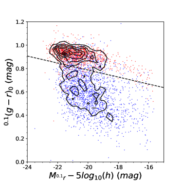
Figure 7: The color-Magnitude diagram for the r-band subsample described in Section 2.3. Red and blue color dots are used to distinguish absorption line galaxies and emission line galaxies. The black contour lines for r-band subsample and a black dashed separation line for the rest-frame bi-modality of galaxies (Zehavi et al. [2011]) are also plotted.

4.2 Dependence of LFs on spectral type

Depending on whether there are obvious emission lines in their spectra, Yang et al. ([2018]) divided galaxies observed in LaCoSSPAr survey into emission line galaxies and absorption line galaxies. The absorption line galaxies sample comprises 1375 typical passive galaxies. Figure 7 presents the color-magnitude diagram of $M_{{}^{0.1}r}$ vs. ${}^{0.1}(g-r)_{0}$ for the r-band subsample described in Section 2.3. Here ${}^{0.1}(g-r)_{0}$ is the rest-frame color for 0.1 blushifted g and r band. Red dots represent the absorption line galaxies and blue dots the emission line galaxies. A contour diagram and a separation line are also overplotted in Figure 7. The color-magnitude separation line (black dashed) is taken from Zehavi et al. ([2011]):

$${}^{0.1}(g-r)_{0}=0.21-0.03\times M_{{}^{0.1}r}$$ (11)

In Figure 8, SWML LFs of SDSS ${}^{0.1}g,^{0.1}r,^{0.1}i$-band for emission line galaxies (blue dots), absorption line galaxies (red dots), and red galaxies (those located above the separation line in Figure 7, red open circle) are plotted, respectively, and are compared to the LFs of the total samples. The absorption line galaxies show higher number densities than emission line galaxies at the luminous end ($Mag_{{}^{0.1}r}$ or $Mag_{{}^{0.1}i}$ $>21.5$ mag) in ${}^{0.1}r$ and ${}^{0.1}i$ bands. In each band, the LF of emission line galaxies appears to have a Schechter function profile with a steeper faint end slope than that of the total sample. As for absorption line galaxies (and red galaxies), the LFs show an obvious dip at $M-5log_{10}h\sim-18.5$ mag in all three bands. A standard Schechter function cannot provide a good fit to the LF of absorption line galaxies over entire magnitude range.

Similar results have been found in many previous works on LFs of passive galaxies in different photometric bands and different redshift ranges (Madgwick et al. [2002]; Wolf et al. [2003]; Blanton et al. [2005]; Salimbeni et al. [2008];  Loveday et al. [2012]; L$\acute{o}$pez-Sanjuan et al. [2017]). Madgwick et al. ([2002]) investigated galaxy luminosity functions for the 2dF survey in $M_{b_{j}}$ band for different spectral types. They divided their galaxies into four spectral types by introducing a new parameter $\eta$, which identifies the average emission and absorption line strength in the galaxy rest-frame spectrum. Their LF for ‘Type 1’ galaxies (absorption line galaxies) shows an obvious dip at $M_{b_{j}}-5log_{10}h\sim-16$ mag.

For comparisons, in Figure 8 we overplot the LFs of red (red dotted lines) and blue galaxies (blue dotted lines) by Loveday et al. ([2012]) in three bands, and by Montero-Dorta & Prada ([2009]) in ${}^{0.1}r$ band (red and blue dashed line). The LFs of blue galaxies of Loveday et al. ([2012]) are in general lower than those of our emission line galaxies. A possible cause for this, beside the difference in definitions of blue galaxies and emission line galaxies, could be the cosmic evolutionary effect because our galaxies have a higher median redshift ($\bar{z}=0.104$) than theirs (all with $z<0.1$) and we did not do any evolutionary correction. For red galaxies, Loveday et al. ([2012]) fitted the LFs with double-power-law Schechter functions, in the form of

$$\phi(M)=0.4ln(10)exp[-10^{-0.4(M-M_{*,S})}]\times\\ \{\phi_{1,S}10^{-0.4(M-M_{*,S})(\alpha_{1,S}+1)}+\\ \phi_{2,S}10^{-0.4(M-M_{*,S})(\alpha_{2,S}+1)}\}.$$ (12)

They show poor agreements with our results for both absorption line galaxies and red galaxies. Montero-Dorta & Prada ([2009]) used the Schechter function to fit their LFs for red and blue galaxies. Their ${}^{0.1}r$ band LF of blue galaxies shows a much better agreement with ours than Loveday et al. ([2012]), but the LF of red galaxies is significantly different from ours.

We found that a double-Gaussian function, as defined in what follows, can provide significantly better fits to the LFs of absorption line galaxies and red galaxies:

$$\phi=\phi_{1,G}exp(-\frac{(M-M_{1,G})^{2}}{2\sigma^{2}_{1,G}})+\phi_{2,G}exp(-\frac{(M-M_{2,G})^{2}}{2\sigma^{2}_{2,G}})$$ (13)

In Figure 9 and Tables 3-4 we compare results of double-Gaussian fittings and double-power-law Schechter function fittings. For absorption line galaxies, the former not only provides a much better fit to the dip at $M_{{}^{0.1}r}-5log_{10}h\sim-18.5$ mag, but also results in smaller reduced-$\chi^{2}$’s in all three bands than the latter. While the double-power-law Schechter function has one characteristic absolute magnitude ($M_{*,S}$), the double-Gaussian function has two characteristic absolute magnitudes $M_{1,G}$ and $M_{2,G}$. This may hint at a bi-modality in the population of absorption line galaxies, with the two sub-populations having distinctively different characteristic luminosities (masses): The more massive sub-population has the luminosity of $L^{*}$ galaxies, while galaxies in the less massive sub-population are $\sim 3.5$ mag (i.e. $\sim 25\times$) fainter.

Peng et al. (2010; 2012) argued that passive galaxies are mainly formed through two distinct processes of “mass quenching" and “environment quenching”. The massive central galaxies (characterized by $L^{*}$ galaxies) are presumably quenched by the first process, and low mass satellite galaxies are quenched by the second process. Is the “bi-modality” of the absorption line galaxies consistent with this theory? To answer this question, we carried out the following test: Firstly we cross-matched our sample of absorption line galaxies with the SDSS-DR7 based NYU-VAGC catalog that Yang et al. (2007) used for group identifications, and then checked the matches for memberships in Yang’s groups. After excluding galaxies associated with one-galaxy groups (i.e. single galaxies) and with groups having no halo mass estimates (uncertain groups), we found 83 absorption line galaxies (70 bright galaxies with $M_{{}^{0.1}r}-5log_{10}h<-18.5$, 13 faint galaxies with $M_{{}^{0.1}r}-5log_{10}h>-18.5$) belonging to 30 groups. Among the 70 bright galaxies (“more massive galaxies”), 26 (37%) are the brightest or the most massive galaxies in their groups, and another 7 (10%) are the second brightest galaxies in groups with three or more members, suggesting that $\sim 50\%$ of these galaxies are the master galaxies in groups. On the other hand, none of the faint galaxies is the brightest neither the most massive galaxy in any group that they belong. Actually, 8 out of the 13 faint absorption line galaxies belong to a single rich group (group-ID 280, with 34 identified members), and indeed they appear to be the “satellite” galaxies in the group, all with the $M_{r}$ rank after the 20th. Our results seem to agree with the hypotheses that the bright and massive absorption line galaxies tend to be master galaxies in groups, while most faint and less massive absorption line galaxies are satellites, consistent with the theory of Peng et al. (2010; 2012). It is worth noting that, because of the poor coverage of the SDSS spectroscopic survey in our fields (Figure 3), only a small fraction of the absorption line galaxies have matches in the NYU-VAGC catalog. Also, the number of faint galaxies (83) is much less than that of bright galaxies (1292) in the absorption line galaxy sample since the finding volume of the former is much smaller than that of the latter.

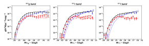
Figure 8: SWML estimates of LFs for emission line galaxies (blue dots and error bars) and absorption line galaxies (red dots and error bars) in ${}^{0.1}g,^{0.1}r,^{0.1}i$ bands in our work. The red unfilled circles are the SWML estimates of LFs for red galaxies corresponding to galaxies located above the separation line in Figure 7. The black dots, error bars and black solid lines are the same as LFs presented in Figure 6. The dashed lines plotted in ${}^{0.1}r$ band are the best fitting Schechter function of LFs for blue galaxies (blue dashed line) and red galaxies (red dashed line) estimated by Montero-Dorta et al. ([2009]). The dotted lines in each band present the LFs for blue (blue dotted line) and red (red dotted line) galaxies at low redshift ($z<0.1$) from Fig. 13 of Loveday et al. ([2012]), which are all fitted with the double-power-law Schechter function.

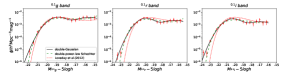
Figure 9: Double-Gaussian function (black solid lines) and double-power-law Schechter function (green dashed lines) fit to LFs of absorption line galaxies in ${}^{0.1}g,^{0.1}r,^{0.1}i$ bands. The red dots are SWML estimates of absorption line galaxies showed in Figure 8. Red dotted lines represent the LFs for red galaxies at low redshift ($z<0.1$) from Fig. 13 of Loveday et al. ([2012]).

Table 3: Least squares fitting parameters of double-Gaussian function to LFs of absorption line galaxies in each band.

Band	$\phi_{1,G}$	$M_{1,G}-5log_{10}h$	$\sigma_{1,G}^{2}$	$\phi_{2,G}$	$M_{2,G}-5log_{10}h$	$\sigma_{2,G}^{2}$	$\chi^{2}_{\nu}$
	$(10^{-2}h^{3}Mpc^{-3})$			$(10^{-2}h^{3}Mpc^{-3})$
${}^{0.1}g$	0.40	-18.95	1.36	0.40	-15.63	3.66	0.66
${}^{0.1}r$	0.34	-20.04	1.53	0.23	-16.50	4.40	0.93
${}^{0.1}i$	0.30	-20.35	1.66	0.18	-16.96	4.40	1.07

Table 4: Least squares fitting parameters of double-power-law Schechter function to LFs of absorption line galaxies in each band.

Band	$M_{*,S}-5log_{10}h$	$\alpha_{1,S}$	$\alpha_{2,S}$	$\phi_{1,S}$	$\phi_{2,S}$	$\chi^{2}_{\nu}$
				$(10^{-5}h^{3}Mpc^{-3})$	$(10^{-2}h^{3}Mpc^{-3})$
${}^{0.1}g$	-19.48	-1.90	-0.53	9.05	0.79	0.80
${}^{0.1}r$	-20.68	-2.03	-0.52	1.91	0.66	1.31
${}^{0.1}i$	-21.16	-2.57	-0.64	0.08	0.53	1.67

5 Summary

LAMOST is one of the most powerful telescopes in accessing the spectra of celestial objects. As a key project of LAMOST, LaCoSSPAr provides the most complete dataset of LAMOST ExtraGAlactic Survey (LEGAS) up to now. In this work, we analyzed the redshift incompleteness in LaCoSSPAr survey quantitatively, and obtained the first measurements of the galaxy LFs in the ${}^{0.1}g$, ${}^{0.1}r$, and ${}^{0.1}i$ bands using LAMOST spectroscopic data.

We used both parametric (STY) and non-parametric (SWML) maximum likelihood methods to construct LFs, and found good agreements between the results. Our LFs are compatible to previous works using SDSS data. Thanks to deeper magnitude limit of LAMOST, compared to results based on SDSS data, we were able to extend the faint end of the LFs by $\sim 1$ mag. Our luminosity densities are consistent with the luminosity density evolution obtained by Loveday et al. ([2012]).

We divided our sample into emission line galaxies and absorption line galaxies, and derived their LFs separately. Our results show that, in every band, the SWML estimate of emission line galaxies LF has a Schechter function profile with a steeper faint end slope than that of the total sample. The LFs of absorption line galaxies show an obvious dip near $\sim 18.5$ mag in all three bands, and cannot be fitted by Schechter functions. On the other hand double-Gaussian functions, with two characteristic absolute magnitudes $M_{1,G}$ and $M_{2,G}$, provide excellent fits to them. This may hint at a bi-modality in the population of absorption line galaxies (representing passive galaxies), with the two sub-populations having distinctively different characteristic luminosities (masses): The more massive sub-population has the luminosity of $L^{*}$ galaxies, while galaxies in the less massive sub-population are $\sim 3.5$ mag (i.e. $\sim 25\times$) fainter. Investigations using the group catalog of Yang et al (2007) indicate that the former tend to be the master galaxies in groups while most of the latter are satellites.

This work is based on a small size galaxy sample within $\sim 40$ $deg^{2}$ survey area which leads to large statistic uncertainties in LF estimates. In the future, we can expect a large-area covering sample when LAMOST finishes its LEGAS survey which can give us a better-constrained and unbiased estimates for LFs.