Novel numerical analysis for simulating the generalized 2D multi-term time fractional Oldroyd-B fluid model

Abstract

In this paper, we consider the finite difference method for the generalized two-dimensional (2D) multi-term time-fractional Oldroyd-B fluid model, which is a subclass of non-Newtonian fluids. Different from the general multi-term time fractional equations, the generalized fluid equation not only has a multi-term time derivative but also possess a special time fractional operator on the spatial derivative. Firstly, a new discretization of the time fractional derivative is given. And a vital lemma, which plays an important role in the proof of stability, is firstly proposed. Then the new finite difference scheme is constructed. Next, the unique solvability, unconditional stability and convergence of the proposed scheme are proved by the energy method. Numerical examples are given to verify the numerical accuracy and efficiency of the numerical scheme as compared to theoretical analysis, and this numerical method can extended to solve other non-Newtonian fluid models.

1 Introduction

In the last few decades, non-Newtonian fluids which do not satisfy a linear relationship between the stress tensor and the deformation tensor have been widely applied in engineering and industry. The constitutive equation of non-Newtonian fluids is much more complex than its Newtonian counterparts, and the constitutive equations involving fractional calculus have been proved to be a valuable tool to handle viscoelastic properties [1, 2] and some results are obtained which are in good agreement with the experimental data [3, 4].

One particular subclass of non-Newtonian fluids is the generalized Oldroyd-B fluid, which has been found to approximate the response to many dilute polymeric liquids. Some recent work regarding the generalized Oldroyd-B fluids can be found in references [5, 6, 7, 8]. The fundamental electromagnetic relations have been summarized by Sutton [9]. For the magnetohydrodynamic(MHD) flow, Zheng et al. [10, 11] discussed the flow between two plates with slip boundary conditions and obtain the exact solution in terms of Fox $H$-function by some transform techniques. Khan et al. [12, 13] investigated the MHD flow of a generalized Oldroyd-B fluid in a circular pipe and a porous space, respectively.

One important part is the following incompressible Oldroyd-B fluid which is bounded by two infinite rigid plates, when a magnetic field is imposed on the above flow under the assumption of low magnetic Reynolds number. Fetecau et al. [14] considered the two dimensional case:

$$(1+\lambda D^{\alpha}_{t})\frac{\partial u(x,y,t)}{\partial t}=\upsilon(1+\theta D^{\beta}_{t})(\frac{\partial^{2}}{\partial x^{2}}+\frac{\partial^{2}}{\partial y^{2}})u(x,y,t),$$

where $\lambda$ and $\theta$ are relaxation and retardation times, $\nu=\frac{\mu}{\rho}$ is the kinematic viscosity of the fluid, $\rho$ is the density of the fluid, $\mu$ is the dynamic viscosity coefficient of the fluid. $D^{\alpha}_{t}$, $D^{\beta}_{t}$ are the time fractional operators, $0<\alpha,\beta<1$ and $u(x,y,t)$ is the velocity. Khan et al. [13] considered the following generalized Oldroyd-B fluid in a porous medium with the influence of Hall current

$$(1+\lambda{D}_{t}^{\alpha})\frac{\partial u(x,t)}{\partial t} =\nu(1+\theta{D}_{t}^{\beta})\frac{\partial^{2}u(x,t)}{\partial x^{2}}-\frac{\nu\varphi_{1}}{k}(1+\theta{D}_{t}^{\beta})u(x,t)$$

$$-\frac{\sigma B_{0}^{2}}{\rho(1-i\phi)}(1+\lambda{D}_{t}^{\alpha})u(x,t),$$

where $k$ is the permeability of the porous medium, $\varphi_{1}$ is the porosity of the medium, $\phi$ is the Hall parameter, $B_{0}$ is the magnetic intensity and $\sigma$ is the electrical conductivity.

Stimulated by the above research in this field, we will give the following two dimensional Oldroyd-B fluid with the influence of Hall current

$$(1+\lambda{D}_{t}^{\alpha})\frac{\partial u(x,y,t)}{\partial t} =\nu(1+\theta{D}_{t}^{\beta})(\frac{\partial^{2}u}{\partial x^{2}}+\frac{\partial^{2}u}{\partial y^{2}})-\frac{\nu\varphi_{1}}{k}(1+\theta{D}_{t}^{\beta})u(x,y,t)$$

$$-\frac{\sigma B_{0}^{2}}{\rho(1-i\phi)}(1+\lambda{D}_{t}^{\alpha})u(x,y,t),$$

we will give the detailed derivation of this fluid model in Section 2.

The research of the incompressible Oldroyd-B fluid is limited to the analytical solution, numerical methods with supporting stability and convergence analysis are limited. In order to give the numerical methods and the discrete scheme, we will consider the following generalized two-dimensional multi-term time fractional non-Newtonian diffusion equation:

$$\sum_{l=1}^{p}a_{l}D^{\gamma_{l}}_{t}u+b_{1}\frac{\partial u}{\partial t}+\sum_{m=1}^{q}c_{m}D^{\alpha_{m}}_{t}u+b_{2}u$$

$$=~{}~{} b_{3}(\frac{\partial^{2}u}{\partial x^{2}}+\frac{\partial^{2}u}{\partial y^{2}})+\sum_{r=1}^{s}d_{r}D^{\beta_{r}}_{t}(\frac{\partial^{2}u}{\partial x^{2}}+\frac{\partial^{2}u}{\partial y^{2}})+f(x,y,t),$$ (1)

where $u=u(x,y,t),$ $(x,y)\in\Omega=(0,L_{x})\times(0,L_{y}),0<t\leq T,$ and with the following initial condition

$$u(x,y,0)=\varphi(x,y),u_{t}(x,y,0)=\phi(x,y),(x,y)\in\Omega$$

and the boundary conditions

$$u(0,y,t)=u(L_{x},y,t)=0,0\leq y\leq L_{y},t>0,$$

$$u(x,0,t)=u(x,L_{y},t)=0,0\leq x\leq L_{x},t>0,$$

where $a_{l}>0,b_{i}>0,c_{m}>0,d_{r}>0,$ $1<\gamma_{l}<2,0<\alpha_{m},\beta_{r}<1$, $l=1,\cdots,p,i=1,2,3,m=1,\cdots,q,r=1,\cdots,s$, and the Caputo time frational derivative $D^{\gamma}_{t}u$, $D^{\alpha}_{t}u$ are given by [15, 16]

$$D^{\gamma}_{t}u=\frac{1}{\Gamma(2-\gamma)}\int_{0}^{t}(t-s)^{1-\gamma}\frac{\partial^{2}u(x,y,s)}{\partial s^{2}}ds,1<\gamma<2,$$

$$D^{\alpha}_{t}u=\frac{1}{\Gamma(1-\alpha)}\int_{0}^{t}(t-s)^{-\alpha}\frac{\partial u(x,y,s)}{\partial s}ds,0<\alpha<1,$$

where $\Gamma(\cdot)$ is the Gamma function.

Although there are some literatures [10, 11, 17, 18] give the analytical solutions of the generalized Oldroyd-B fluid, but they are always given in series form with generalized G or $H$-function. Therefore, numerical method is a promising tool to solve these equations. And up to now, numerical methods to solve fractional diffusion equation mainly are finite difference methods [19, 20, 21, 22, 23, 24, 25], finite element method [26, 27, 28, 29], finite volume methods [30, 31], spectral methods [32, 33, 34] and meshless methods [35, 36]. Bazhlekova et al. [37] proposed a finite difference method to solve the viscoelastic flow with generalized fractional Oldroyd-B model, fractional operator is Riemann-Liouville time fractional derivative and they utilised the Grünwald-Letnikov formula to approximate it, which was low accuracy and lacked theoretical analysis. Recently, Feng et al. [38] gave the numerical solution to these problems, but it confined to one-dimensional case, the two-dimensional case is seldom solved, and the temporal convergence order we get in this paper is ${\min\{3-\gamma_{l},2-\alpha_{m},2-\beta_{r}\}}$, this is also better than [38] which the temporal convergence is only first order.

The outline of the paper is as follows. In section 2, preliminary knowledge is given, in which a new numerical scheme to discretise the time fractional derivative is proposed. In section 3, we develop the finite difference method for the generalized Oldroyd-B fluid model and derive the implicit scheme. And we proceed with the proof of the stability and convergence of the scheme by energy method and discuss the solvability of the numerical scheme in section 4. In section 5, we present two numerical examples to demonstrate the effectiveness of our method and some conclusions are drawn finally.

2 Formulation of the Multi-term time fractional flow model

We impose a magnetic field in the positive $y$-axis with intensity $B_{0}$ and the electrical conductivity is $\sigma$. Suppose that the main flow only takes place along the $x-$axis, then we shall assume the velocity field and the extra stress of the form

$$\textbf{V}=\textbf{V}(x,y,t)=u(x,y,t)\textbf{i},~{}\textbf{S}=\textbf{S}(x,y,t)=S(x,y,t)\textbf{i}$$ (2)

where i is the unit vector in the $z-$direction of the Cartesian coordinate system $x,y$ and $z$.

The conservation equation of an incompressible fluid is

$$div\textbf{V}=0,$$ (3)

$$\rho\frac{d\textbf{V}}{dt}=-\nabla P+div\textbf{S}+\textbf{J}\times\textbf{B}+\textbf{r},$$ (4)

where $\rho$ is the fluid density, $P$ is the hydrostatic pressure, $\nabla$ is the gradient operator, r is the Darcy resistance for an Oldroyd-B fluid, and J is the current density, B is the total magnetic field so that $\textbf{B}=\textbf{B}_{0}+\textbf{b}$, $\textbf{B}_{0}$ and b are the applied and induced magnetic fields, respectively. By Eq.(2), the continuous equation (3) holds automatically. The constitutive equation for a generalized Oldroyd-B fluid is defined as[15]:

$$(1+\lambda\frac{D^{\alpha}}{Dt^{\alpha}})\textbf{S}=\mu(1+\theta\frac{D^{\beta}}{Dt^{\beta}})\textbf{A},\quad(0<\alpha,\beta<1)$$ (5)

where $\mu$ is the dynamic viscosity and $\lambda$ and $\theta$ are relaxation and retardation times, and $\alpha$ and $\beta$ are fractional calculus orders, and $\textbf{A}=\textbf{L}+\textbf{L}^{T}(\textbf{L}=\nabla\textbf{V})$ denotes the first Rivlin-Ericksen tensor. The material derivative operators $\frac{D^{\alpha}}{Dt^{\alpha}}$ and $\frac{D^{\beta}}{Dt^{\beta}}$ can be expressed as

$$\frac{D^{\alpha}}{Dt^{\alpha}}\textbf{S}=D^{\alpha}_{t}\textbf{S}+(\textbf{V}\cdot\nabla)\textbf{S}-\textbf{L}\textbf{S}-\textbf{S}\textbf{L}^{T},$$ (6)

$$\frac{D^{\beta}}{Dt^{\beta}}\textbf{A}=D^{\beta}_{t}\textbf{A}+(\textbf{V}\cdot\nabla)\textbf{A}-\textbf{L}\textbf{A}-\textbf{A}\textbf{L}^{T},$$ (7)

where $D^{\alpha}_{t}$ and $D^{\beta}_{t}$ are the Caputo fractional derivative operators of order $\alpha$ and $\beta$ with respect to $t$, respectively. $\theta=0$ we have a generalized Maxwell fluid. The classical Navier-Stokes fluid can be obtained for $\lambda=\theta=0$ and $\alpha=\beta=1$. The Hall effect is taken into consideration, and thus we have

$$\textbf{J}\times\frac{\omega_{e}\tau_{e}}{B_{0}}(\textbf{J}\times\textbf{B})=\sigma[\textbf{E}+\textbf{V}\times\textbf{B}\times\frac{1}{en_{e}}\bigtriangledown p_{e}],$$ (8)

in which $\omega_{e}$ is the cyclotron frequency of electrons, $\tau_{e}$ is the electron collision time, $\sigma$ is the electrical conductivity, $e$ is the electron charge, $n_{e}$ is the number density of electrons and $p_{e}$ is the electron pressure, E is the electric field. Further, it is assumed that there is no applied or polarization voltage so that $\textbf{E}=0$.

Moreover, Darcy resistance r can also be interpreted as measure of the flow resistance offered by the solid matrix, thus r satisfies the following equation:

$$(1+\lambda\frac{D^{\alpha}}{Dt^{\alpha}})\textbf{r}=-\frac{\mu\phi_{1}}{k}(1+\theta\frac{D^{\beta}}{Dt^{\beta}})\textbf{V}.$$ (9)

where $\phi_{1}$ is the porosity of the medium.

Substituting (6) and (7) into (5) and taking into account the initial condition $\textbf{S}(x,y,0)=0$, we obtain $S_{xx}=S_{xy}=S_{yy}=0$ and the relevant partial differential equations

$$(1+\lambda D_{t}^{\alpha})S_{zx}=\mu(1+\theta D_{t}^{\beta})\frac{\partial u}{\partial x},~{}(1+\lambda D_{t}^{\alpha})S_{zy}=\mu(1+\theta D_{t}^{\beta})\frac{\partial u}{\partial y},$$ (10)

then substituting Eqs.(8-10) into Eq.(4) and neglecting the pressure gradient, then we obtain the generalized two dimensional Oldroyd-B fluid with the influence of Hall current.

3 Preliminary

Firstly, in the $x-$direction $[0,L_{x}]$, we take the mesh points $x_{i}=ih_{x}$, $i=0,1,\cdots,M_{x}$, in the $y-$direction $[0,L_{y}]$, we take the mesh points $y_{j}=jh_{y}$, $j=0,1,\cdots,M_{y}$, and $t_{n}=n\tau$, $n=0,1,\cdots,N$, where $h_{x}=L_{x}/M_{x}$,$h_{y}=L_{y}/M_{y}$, $\tau=T/N$ are the uniform spatial step size and temporal step size, respectively. Denote $\Omega_{\tau}\equiv\{t_{n}|~{}0\leq n\leq N\}$, $\Omega_{h}\equiv\{(x_{i},y_{j})|~{}0\leq i\leq M_{x},0\leq j\leq M_{y}\}$. Suppose $u_{ij}^{n}=u(x_{i},y_{j},t_{n})$, $u_{ij}^{n}$ is a grid function on $\Omega_{h}\times\Omega_{\tau}$. We introduce the following notations:

$$\nabla_{t}u_{ij}^{n}=\frac{u_{ij}^{n}-u_{ij}^{n-1}}{\tau},\quad u_{ij}^{n-\frac{1}{2}}=\frac{u_{ij}^{n}+u_{ij}^{n-1}}{2},\quad\nabla_{x}u_{ij}^{n}=\frac{u_{ij}^{n}-u_{i-1j}^{n}}{h},$$

$$\delta_{x}^{2}u_{ij}^{n}=\frac{u_{i-1j}^{n}-2u_{ij}^{n}+u_{i+1j}^{n}}{h_{x}^{2}},\quad\delta_{y}^{2}u_{ij}^{n}=\frac{u_{ij-1}^{n}-2u_{ij}^{n}+u_{ij+1}^{n}}{h_{y}^{2}}.$$

For improving the temporal convergence accuracy from first order [38] to higher order, we will give a new discretization of the fractional derivative ${D_{t}^{\alpha}}u$ $(0<\alpha<1)$. For the function $u\in C^{0,0,3}_{x,y,t}(\Omega\times(0,T])$ at the point$(x_{i},y_{j},t_{n-\frac{1}{2}})$, then the following equality holds

$${D_{t}^{\alpha}}u(\cdot,t_{n-\frac{1}{2}}) =\frac{1}{\Gamma(1-\alpha)}\int_{0}^{t_{n-\frac{1}{2}}}\frac{\partial_{\eta}u(\cdot,\eta)d\eta}{(t_{n-\frac{1}{2}}-\eta)^{\alpha}}$$

$$=\frac{1}{\Gamma(1-\alpha)}\sum_{k=1}^{n-1}\int_{t_{k-1}}^{t_{k}}\frac{\partial_{\eta}u(\cdot,\eta)d\eta}{(t_{n-\frac{1}{2}}-\eta)^{\alpha}}$$

$$+\frac{1}{\Gamma(1-\alpha)}\int_{t_{n-1}}^{t_{n-\frac{1}{2}}}\frac{\partial_{\eta}u(\cdot,\eta)d\eta}{(t_{n-\frac{1}{2}}-\eta)^{\alpha}},$$ (11)

where $u(\cdot,t)$ denotes $u(x_{i},y_{j},t).$ On each interval $[t_{k-1},t_{k}](1\leq k\leq n-1)$, denoting the quadratic interpolation $\Pi_{2,k}u(\cdot,t)$ of $u(\cdot,t)$ using three points $(t_{k-1},u(\cdot,t_{k-1}))$, $(t_{k},u(\cdot,t_{k}))$ and $(t_{k+1},u(\cdot,t_{k+1}))$, we get

$$\Pi_{2,k}u(\cdot,t) =u(\cdot,t_{k-1})\frac{(t-t_{k})(t-t_{k+1})}{2\tau^{2}}-u(\cdot,t_{k})\frac{(t-t_{k-1})(t-t_{k+1})}{\tau^{2}}$$

$$+u(\cdot,t_{k+1})\frac{(t-t_{k-1})(t-t_{k})}{2\tau^{2}},$$ (12)

on the interval $[t_{n-1},t_{n-\frac{1}{2}}]$, denoting the linear interpolation $\Pi_{1,n}u(\cdot,t)$ of $u(\cdot,t)$ using two points $(t_{n-1},u(\cdot,t_{n-1}))$ and $(t_{n},u(\cdot,t_{n}))$, we get

$$\Pi_{1,n}u(\cdot,t)=u(\cdot,t_{n})\frac{(t-t_{n})}{\tau}-u(\cdot,t_{n-1})\frac{(t-t_{n-1})}{\tau},$$ (13)

similar to the calculation in [39], we obtain the difference analog of the Caputo fractional derivative of the order $\alpha~{}(0<\alpha<1)$ for the function $u(x,y,t)$ in the following form:

$$D_{t}^{\alpha}u(\cdot,t_{n-\frac{1}{2}}) =\frac{1}{\Gamma(1-\alpha)}\sum_{k=1}^{n-1}\int_{t_{k-1}}^{t_{k}}\frac{\partial_{\eta}(\Pi_{2,k}u(\cdot,\eta))d\eta}{(t_{n-\frac{1}{2}}-\eta)^{\alpha}}$$ (14)

$$+\frac{1}{\Gamma(1-\alpha)}\int_{t_{n-1}}^{t_{n-\frac{1}{2}}}\frac{\partial_{\eta}(\Pi_{1,n}u(\cdot,\eta))d\eta}{(t_{n-\frac{1}{2}}-\eta)^{\alpha}}+R_{1}$$

$$=\frac{\tau^{-\alpha}}{\Gamma(2-\alpha)}\Big{[}c_{0}^{(\alpha)}u_{ij}^{n}-\sum_{k=1}^{n-1}(c_{n-k-1}^{(\alpha)}-c_{n-k}^{(\alpha)})u_{ij}^{k}-c_{n-1}^{(\alpha)}u_{ij}^{0}\Big{]}+R_{1}$$

$$=\frac{\tau^{1-\alpha}}{\Gamma(2-\alpha)}\sum^{n}_{k=1}c_{n-k}^{(\alpha)}\nabla_{t}u_{ij}^{k}+R_{1},$$

where $R_{1}$ is the error, and for $n=1$

$$c_{0}^{(\alpha)}=a_{0}^{(\alpha)},$$ (15)

for $n\geq 2$,

$$c_{k}^{(\alpha)}=\left\{\begin{aligned} &a_{0}^{(\alpha)}+b_{1}^{(\alpha)},\qquad\qquad k=0,\\ &a_{k}^{(\alpha)}+b_{k+1}^{(\alpha)}-b_{k}^{(\alpha)},~{}~{}1\leq k\leq n-2,\\ &a_{k}^{(\alpha)}-b_{k}^{(\alpha)},\qquad\qquad k=n-1,\end{aligned}\right.$$ (16)

where $a_{0}^{(\alpha)}=(\frac{1}{2})^{1-\alpha},a_{k}^{(\alpha)}=(k+\frac{1}{2})^{1-\alpha}-(k-\frac{1}{2})^{1-\alpha},k\geq 1,$ and $b_{k}^{(\alpha)}=\frac{1}{2-\alpha}\Big{[}(k+\frac{1}{2})^{2-\alpha}-(k-\frac{1}{2})^{2-\alpha}\Big{]}-\frac{1}{2}\Big{[}(k+\frac{1}{2})^{1-\alpha}+(k-\frac{1}{2})^{1-\alpha}\Big{]},k\geq 1.$

Lemma 3.1.

For any $0<\alpha<1$ and $u\in C^{0,0,3}_{x,y,t}(\Omega\times(0,T])$, the error

$$|R_{1}|=|D_{t}^{\alpha}u(\cdot,t_{n-\frac{1}{2}})-\frac{\tau^{1-\alpha}}{\Gamma(2-\alpha)}\sum^{n}_{k=1}c_{n-k}^{(\alpha)}\nabla_{t}u_{ij}^{k}|=O(\tau^{2-\alpha}),$$ (17)

Proof.

Let $R_{1}=R_{1}^{n-1}+R_{n-1}^{n-\frac{1}{2}}$, where

$$R_{1}^{n-1} =\frac{1}{\Gamma(1-\alpha)}\sum_{k=1}^{n-1}\int_{t_{k}}^{t_{k+1}}\frac{\partial_{\eta}(u(\cdot,\eta)-\Pi_{2,k}u(\cdot,\eta))d\eta}{(t_{n-\frac{1}{2}}-\eta)^{\alpha}},$$

$$R_{n-1}^{n-\frac{1}{2}} =\frac{1}{\Gamma(1-\alpha)}\int_{t_{n-1}}^{t_{n-\frac{1}{2}}}\frac{\partial_{\eta}(u(\cdot,\eta)-\Pi_{1,n}u(\cdot,\eta))d\eta}{(t_{n-\frac{1}{2}}-\eta)^{\alpha}},$$

we estimate the error $R_{1}^{n-1}$ similarly to [39]:

$$R_{1}^{n-1}\leq\frac{2^{\alpha}|\partial_{t}^{3}u(\cdot,\xi)|}{3\Gamma(1-\alpha)}\tau^{3-\alpha},$$

and

$$R_{n-1}^{n-\frac{1}{2}} =\frac{1}{\Gamma(1-\alpha)}\int_{t_{n-1}}^{t_{n-\frac{1}{2}}}\frac{(\partial_{\eta}u(\cdot,\eta)-\frac{u(\cdot,t_{n})-u(\cdot,t_{n-1})}{\tau})d\eta}{(t_{n-\frac{1}{2}}-\eta)^{\alpha}}$$

$$=\frac{1}{\Gamma(1-\alpha)}\int_{t_{n-1}}^{t_{n-\frac{1}{2}}}\frac{(\partial_{\eta}u(\cdot,t_{n-\frac{1}{2}})-\frac{u(\cdot,t_{n})-u(\cdot,t_{n-1})}{\tau})d\eta}{(t_{n-\frac{1}{2}}-\eta)^{\alpha}}+O(\tau^{2-\alpha})$$

$$=O(\tau^{2-\alpha}),$$

then the error $|R_{1}|=O(\tau^{2-\alpha})$, Lemma 1 is proved. ∎

The new discretization of ${D_{t}^{\alpha}}u$ $(0<\alpha<1)$ will help us improve the temporal convergence accuracy of the Eq.(1) from $\tau$ [38] to $\tau^{\min\{3-\gamma_{l},2-\alpha_{m},2-\beta_{r}\}}$.

Lemma 3.2.

The coefficients $a_{k}^{(\alpha)}(k=0,1,2,\ldots,n)$ and $b_{k}^{(\alpha)}(k=1,2,\ldots,n)$ satisfy the following properties:

• $a_{k}^{(\alpha)}>0,\lim\limits_{k\rightarrow\infty}a_{k}^{(\alpha)}=0$;  $a_{k}^{(\alpha)}>a_{k+1}^{(\alpha)},k\geq 1$;  $a_{k+1}^{(\alpha)}-2a_{k}^{(\alpha)}+a_{k-1}^{(\alpha)}\geq 0,$ $k\geq 2$,

• $b_{k}^{(\alpha)}>0;$  $\lim\limits_{k\rightarrow\infty}b_{k}^{(\alpha)}=0$;  $b_{k}^{(\alpha)}>b_{k+1}^{(\alpha)}.$

Proof.

Similar to the proof in [39]. ∎

Lemma 3.3.

The coefficients $c_{k}^{(\alpha)}(k=0,1,2,\ldots,n-1)$ satisfy the following properties:

• $c_{k}^{(\alpha)}>0$, $\lim\limits_{k\rightarrow\infty}c_{k}^{(\alpha)}=0$,

• $c_{0}^{(\alpha)}>c_{1}^{(\alpha)}>\cdots>c_{n-2}^{(\alpha)}>c_{n-1}^{(\alpha)}$,

• $c_{k+1}^{(\alpha)}-2c_{k}^{(\alpha)}+c_{k-1}^{(\alpha)}>0,~{}k\geq 2,$$~{}k\neq n-2.$

Proof.

Similar to the proof in [39], the properties (1)-(2) are easy to get. Let us prove the property (3).

For $k\geq 2$ and $k+1\neq n-1$ we have

$${c_{k+1}^{(\alpha)}-2c_{k}^{(\alpha)}+c_{k-1}^{(\alpha)}=(a_{k+1}^{(\alpha)}+b_{k+2}^{(\alpha)}-b_{k+1}^{(\alpha)})-2(a_{k}^{(\alpha)}+b_{k+1}^{(\alpha)}-b_{k}^{(\alpha)})+(a_{k-1}^{(\alpha)}+b_{k}^{(\alpha)}-b_{k-1}^{(\alpha)})}$$

$$=\frac{1}{2-\alpha}\big{[}(k+\frac{5}{2})^{2-\alpha}-4(k+\frac{3}{2})^{2-\alpha}+6(k+\frac{1}{2})^{2-\alpha}-4(k-\frac{1}{2})^{2-\alpha}+(k-\frac{3}{2})^{2-\alpha}\big{]}$$

$$-\frac{1}{2}\big{[}(k+\frac{5}{2})^{1-\alpha}-4(k+\frac{3}{2})^{1-\alpha}+6(k+\frac{1}{2})^{1-\alpha}-4(k-\frac{1}{2})^{1-\alpha}+(k-\frac{3}{2})^{1-\alpha}\big{]}$$

$$=\alpha(1-\alpha)(1+\alpha)\int_{0}^{1}dz_{1}\int_{0}^{1}dz_{2}\int_{0}^{1}dz_{3}\int_{0}^{1}\frac{dz_{4}}{(k-\frac{3}{2}+z_{1}+z_{2}+z_{3}+z_{4})^{2+\alpha}}$$

$$+\frac{\alpha(1-\alpha)(1+\alpha)(2+\alpha)}{2}\int_{0}^{1}dz_{1}\int_{0}^{1}dz_{2}\int_{0}^{1}dz_{3}\int_{0}^{1}\frac{dz_{4}}{(k-\frac{3}{2}+z_{1}+z_{2}+z_{3}+z_{4})^{3+\alpha}}$$

$$>\alpha(1-\alpha)(1+\alpha)\frac{1}{(k+\frac{5}{2})^{2+\alpha}}+\frac{\alpha(1-\alpha)(1+\alpha)(2+\alpha)}{2}\frac{1}{(k+\frac{5}{2})^{3+\alpha}}>0,$$

formula $h^{\prime}(z)<0$. Consequently, $c_{n}^{(n+1,\alpha)}>c_{n+1}^{(n+2,\alpha)},n\geq 1$. the proof is completed. ∎

Remark 1: When $c_{2}^{(\alpha)}-2c_{1}^{(\alpha)}+c_{0}^{(\alpha)}$ is a formula of parameter $\alpha$, but it is not always greater than 0, by simple algebraic calculation, when $0<\alpha<0.4471$, $c_{2}^{(\alpha)}-2c_{1}^{(\alpha)}+c_{0}^{(\alpha)}<0$, else $c_{2}^{(\alpha)}-2c_{1}^{(\alpha)}+c_{0}^{(\alpha)}>0$.

Similarly, for the time fractional derivative ${D_{t}^{\beta}}u$ $(0<\beta<1)$, we use the following formula

$${D_{t}^{\beta}}u(\cdot,t_{n-\frac{1}{2}}) =\frac{\tau^{-\beta}}{\Gamma(2-\beta)}\Big{[}c_{0}^{(\beta)}u_{ij}^{n}-\sum_{k=1}^{n-1}(c_{n-k-1}^{(\beta)}-c_{n-k}^{(\beta)})u_{ij}^{k}-c_{n-1}^{(\beta)}u_{ij}^{0}\Big{]}+R_{2},$$ (18)

$$=\frac{\tau^{1-\beta}}{\Gamma(2-\beta)}\sum^{n}_{k=1}c_{n-k}^{(\beta)}\nabla_{t}u_{ij}^{k}+R_{2},$$

where $R_{2}=O(\tau^{2-\beta})$ and the coefficients are similar to Lemma 2 and Lemma 3.

Next, we will give the new scheme for the fractional derivative ${D_{t}^{\beta}}(\partial_{x}^{2}+\partial_{y}^{2})u,$ $0<\beta<1$.

Since

$${D_{t}^{\beta}}(\partial_{x}^{2}+\partial_{y}^{2})u(\cdot,t_{n-\frac{1}{2}}) =(\delta_{x}^{2}+\delta_{y}^{2})u(\cdot,t_{n-\frac{1}{2}})$$

$$-\frac{h_{x}^{2}}{12}\frac{\partial^{4}u(\xi_{i},y_{j},t_{n-\frac{1}{2}})}{\partial x^{4}}-\frac{h_{y}^{2}}{12}\frac{\partial^{4}u(x_{i},\varsigma_{j},t_{n-\frac{1}{2}})}{\partial y^{4}},$$

where $x_{i-1}\leq\xi_{i}\leq x_{i},y_{j-1}\leq\varsigma_{j}\leq y_{j}$, then we have

$${D_{t}^{\beta}}(\partial_{x}^{2}+\partial_{y}^{2})u(\cdot,t_{n-\frac{1}{2}}) =\frac{\tau^{-\beta}}{\Gamma(2-\beta)}\Big{[}c_{0}^{(\beta)}(\partial_{x}^{2}+\partial_{y}^{2})u(\cdot,t_{n})$$

$$-\sum_{k=1}^{n-1}(c_{n-k-1}^{(\beta)}-c_{n-k}^{(\beta)})(\partial_{x}^{2}+\partial_{y}^{2})u(\cdot,t_{k})$$

$$-c_{n-1}^{(\beta)}(\partial_{x}^{2}+\partial_{y}^{2})u(\cdot,0)\Big{]}+R_{3},$$

$$=\frac{\tau^{-\beta}}{\Gamma(2-\beta)}\Big{[}c_{0}^{(\beta)}(\delta_{x}^{2}+\delta_{y}^{2})u(\cdot,t_{n})$$

$$-\sum_{k=1}^{n-1}(c_{n-k-1}^{(\beta)}-c_{n-k}^{(\beta)})(\delta_{x}^{2}+\delta_{y}^{2})u(\cdot,t_{k})$$

$$-c_{n-1}^{(\beta)}(\delta_{x}^{2}+\delta_{y}^{2})u(\cdot,0)\Big{]}+R_{4}+R_{3},$$

where $|R_{3}|\leq C\tau^{2-\beta}$ and

$$R_{4} =-\frac{h_{x}^{2}\tau^{-\beta}}{12\Gamma(2-\beta)}\sum_{k=0}^{n-1}c_{k}^{(\beta)}\Big{[}\frac{\partial^{4}u(\xi_{i},y_{j},t_{n-k})}{\partial x^{4}}-\frac{\partial^{4}u(\xi_{i},y_{j},t_{n-k-1})}{\partial x^{4}}\Big{]}$$

$$-\frac{h_{y}^{2}\tau^{-\beta}}{12\Gamma(2-\beta)}\sum_{k=0}^{n-1}c_{k}^{(\beta)}\Big{[}\frac{\partial^{4}u(x_{i},\varsigma_{j},t_{n-k})}{\partial y^{4}}-\frac{\partial^{4}w(x_{i},\varsigma_{j},t_{n-k-1})}{\partial y^{4}}\Big{]}$$

$$=-\frac{h_{x}^{2}\tau^{1-\beta}}{12\Gamma(2-\beta)}\sum_{k=0}^{n-1}c^{(\beta)}_{k}\frac{\partial^{5}u(\xi_{i},y_{j},\eta_{n-k})}{\partial x^{4}\partial t}-\frac{h_{y}^{2}\tau^{1-\beta}}{12\Gamma(2-\beta)}\sum_{k=0}^{n-1}c^{(\beta)}_{k}\frac{\partial^{5}u(x_{i},\varsigma_{j},\upsilon_{n-k})}{\partial y^{4}\partial t},$$

where $t_{n-k-1}<\eta_{n-k},\upsilon_{n-k}<t_{n-k}$.

$$|R_{4}| \leq\frac{\tau^{1-\beta}}{12\Gamma(2-\beta)}\big{(}h_{x}^{2}\max_{\begin{subarray}{c}(x,y)\in\Omega\\ t\in(0,T]\end{subarray}}\bigg{|}\frac{\partial^{5}u(\xi_{i},y_{j},\eta_{n-k})}{\partial x^{4}\partial t}\bigg{|}+h_{y}^{2}\max_{\begin{subarray}{c}(x,y)\in\Omega\\ t\in(0,T]\end{subarray}}\bigg{|}\frac{\partial^{5}u(x_{i},\varsigma_{j},\upsilon_{n-k})}{\partial y^{4}\partial t}\bigg{|}\big{)}\sum_{k=0}^{n-1}c_{k}^{(\beta)}$$

$$=\frac{\tau^{1-\beta}}{12\Gamma(2-\beta)}\big{(}h_{x}^{2}\max_{\begin{subarray}{c}(x,y)\in\Omega\\ t\in(0,T]\end{subarray}}\bigg{|}\frac{\partial^{5}u(\xi_{i},y_{j},\eta_{n-k})}{\partial x^{4}\partial t}\bigg{|}+h_{y}^{2}\max_{\begin{subarray}{c}(x,y)\in\Omega\\ t\in(0,T]\end{subarray}}\bigg{|}\frac{\partial^{5}u(x_{i},\varsigma_{j},\upsilon_{n-k})}{\partial y^{4}\partial t}\bigg{|}\big{)}\sum_{k=0}^{n-1}a_{k}^{(\beta)}$$

$$=\frac{\tau^{1-\beta}}{12\Gamma(2-\beta)}\big{(}h_{x}^{2}\max_{\begin{subarray}{c}(x,y)\in\Omega\\ t\in(0,T]\end{subarray}}\bigg{|}\frac{\partial^{5}u(\xi_{i},y_{j},\eta_{n-k})}{\partial x^{4}\partial t}\bigg{|}+h_{y}^{2}\max_{\begin{subarray}{c}(x,y)\in\Omega\\ t\in(0,T]\end{subarray}}\bigg{|}\frac{\partial^{5}u(x_{i},\varsigma_{j},\upsilon_{n-k})}{\partial y^{4}\partial t}\bigg{|}\big{)}\cdot(n-\frac{1}{2})^{1-\beta}$$

$$\leq\frac{T^{1-\beta}}{12\Gamma(2-\beta)}\big{(}h_{x}^{2}\max_{\begin{subarray}{c}(x,y)\in\Omega\\ t\in(0,T]\end{subarray}}\bigg{|}\frac{\partial^{5}u(\xi_{i},y_{j},\eta_{n-k})}{\partial x^{4}\partial t}\bigg{|}+h_{y}^{2}\max_{\begin{subarray}{c}(x,y)\in\Omega\\ t\in(0,T]\end{subarray}}\bigg{|}\frac{\partial^{5}u(x_{i},\varsigma_{j},\upsilon_{n-k})}{\partial y^{4}\partial t}\bigg{|}\big{)},$$

then we have

$${D_{t}^{\beta}}(\partial_{x}^{2}+\partial_{y}^{2})u(\cdot,t_{n-\frac{1}{2}})=\frac{\tau^{1-\beta}}{\Gamma(2-\beta)}\sum^{n}_{k=1}c_{n-k}^{(\beta)}\nabla_{t}(\delta_{x}^{2}+\delta_{y}^{2})u_{ij}^{k}+R_{5},$$ (19)

where $R_{5}\leq C(\tau^{2-\beta}+h_{x}^{2}+h_{y}^{2})$.

Lemma 3.4.

For $0<\alpha<1$, $c_{k}^{(\alpha)}$ is defined as (15),(16), and for any positive integer $N$ and real vector $\mathbf{Q}=(v^{1},v^{2},\ldots,v^{N-1},v^{N})\in R^{N+1}$, we have

$$\sum_{n=1}^{N}\sum_{k=1}^{n}c_{n-k}^{(\alpha)}\,v^{k}v^{n}\geq 0.$$ (20)

Analyse: This is the vital Lemma, which plays an important role in the proof of unconditional stability. In the literature [42], the real sequence ${a_{0},a_{1},\cdots,a_{n},\cdots}$ satisfy $a_{n+1}-2a_{n}+a_{n-1}\geq 0,n=1,2,\cdots$. But from the Remark 1, the coefficients $c_{2}^{(\alpha)}-2c_{1}^{(\alpha)}+c_{0}^{(\alpha)}$ is not always greater than $0$. Next, we will give the proof that it does not affect the results. Then similar to Proposition 5.1 [42], we will first prove the following results.

For the coefficients $c_{k}^{(\alpha)}$ is defined as (16),(17), if

$$\lim\limits_{M\rightarrow\infty}c_{M+1}^{(\alpha)}\sum\limits_{k=0}\limits^{M}\cos(kx)\geq 0,$$

(the limit may be $+\infty$), then

$$\sum\limits_{k=0}\limits^{\infty}c_{k}^{(\alpha)}\cos(kx)>0$$

(and the sum of the series may be $+\infty$).

Proof.

For each nonnegative integer $M$, we define $A_{M}=\sum\limits_{k=0}\limits^{M}c_{k}^{(\alpha)}\cos(kx)$, by summing by parts twice, we arrive at

$$A_{M} =c_{M+1}^{(\alpha)}\sum\limits_{k=0}\limits^{M}\cos(kx)-(c_{M+2}^{(\alpha)}-c_{M+1}^{(\alpha)})\sum\limits_{k=0}\limits^{M}\sum\limits_{p=0}\limits^{k}\cos(px)$$

$$+\sum\limits_{k=0}\limits^{M}(c_{k+2}^{(\alpha)}-2c_{k+1}^{(\alpha)}+c_{k}^{(\alpha)})$$

$$+\sum\limits_{k=1}\limits^{M}(c_{k+2}^{(\alpha)}-2c_{k+1}^{(\alpha)}+c_{k}^{(\alpha)})\sum\limits_{p=1}\limits^{k}\sum\limits_{m=0}\limits^{p}\cos(mx).$$

From the well-known identity

$$\sum\limits_{m=0}\limits^{p}\cos(mx)=\left\{\begin{aligned} &\frac{1-\cos x+\cos(px)-\cos(p+1)x}{2(1-\cos x)},~{}\cos x\neq 1,\\ &p+1,\qquad\qquad\qquad\qquad~{}~{}~{}~{}~{}~{}~{}~{}~{}~{}~{}~{}~{}~{}\cos x=1.\end{aligned}\right.$$

by induction we get

$$\sum\limits_{p=0}\limits^{k}\sum\limits_{m=0}\limits^{p}\cos(mx) =\left\{\begin{aligned} &\frac{(k+2)-(k+1)\cos x-\cos(k+1)x}{2(1-\cos x)},~{}\cos x\neq 1\\ &\frac{(k+2)(k+1)}{2},\qquad\qquad\qquad\qquad~{}~{}~{}~{}~{}~{}\cos x=1\end{aligned}\right.$$

$$\geq 0,$$

and

$$\sum\limits_{p=1}\limits^{k}\sum\limits_{m=0}\limits^{p}\cos(mx) =\left\{\begin{aligned} &\frac{k-(k-1)\cos x-\cos(k+1)x}{2(1-\cos x)},~{}\cos x\neq 1\\ &\frac{k(k+3)}{2},\qquad\qquad\qquad\qquad~{}~{}~{}~{}~{}~{}\cos x=1\end{aligned}\right.$$

$$\geq 0.$$

From the properties of $c_{k}^{(\alpha)}$ in Lemma 3,

$$\lim\limits_{M\rightarrow\infty}\sum\limits_{k=0}\limits^{M}(c_{k+2}^{(\alpha)}-2c_{k+1}^{(\alpha)}+c_{k}^{(\alpha)}) =\lim\limits_{M\rightarrow\infty}(c_{0}^{(\alpha)}-c_{1}^{(\alpha)}+c_{M+2}^{(\alpha)}-c_{M+1}^{(\alpha)})$$

$$=c_{0}^{(\alpha)}-c_{1}^{(\alpha)}>0,$$

it is clear that $\sum\limits_{k=0}\limits^{\infty}c_{k}^{(\alpha)}\cos(kx)>0.$ ∎

Next one makes the same proof to Proposition 5.2 [42], (21) is proved.

Next we give the following lemmas [43].

Lemma 3.5.

Discretization of the time fractional derivative ${D_{t}^{\gamma}}u(x,y,t)$ $(1<\gamma<2)$. From the results in [43], at mesh points $(x_{i},y_{j},t_{n-\frac{1}{2}})$ we get

$${D_{t}^{\gamma}}u(x_{i},y_{j},t_{n-\frac{1}{2}}) \approx\frac{1}{2}[D_{t}^{\gamma}u(x_{i},y_{j},t_{n})+D_{t}^{\gamma}u(x_{i},y_{j},t_{n-1})\big{]}$$ (21)

$$=\frac{\tau^{1-\gamma}}{\Gamma(3-\gamma)}\Big{[}a_{0}^{(\gamma)}\nabla_{t}u_{ij}^{n}-\sum_{k=1}^{n-1}(a_{n-k-1}^{(\gamma)}-a_{n-k}^{(\gamma)})\nabla_{t}u_{ij}^{k}$$

$$-a_{n-1}^{(\gamma)}\frac{\partial u(x_{i},y_{j},0)}{\partial t}\Big{]}+R_{8},$$

where $R_{8}=O(\tau^{3-\gamma})$, the coefficients $a_{k}^{(\gamma)}=(k+1)^{2-\gamma}-k^{2-\gamma}$, $k=0,1,2,\ldots$ and satisfy the following properties:

• $a_{k}^{(\gamma)}>0$, $a_{0}^{(\gamma)}=1$, $a_{k}^{(\gamma)}>a_{k+1}^{(\gamma)}$, ${\lim\limits_{k\to\infty}}a_{k}^{(\gamma)}=0$,

• $\sum\limits_{k=0}^{n-1}(a_{k}^{(\gamma)}-a_{k+1}^{(\gamma)})+a_{n}^{(\gamma)}=1$,

• $(2-\gamma)(k+1)^{1-\gamma}\leq a_{k}^{(\gamma)}\leq(2-\gamma)k^{1-\gamma}$.

Lemma 3.6 ([38]).

For $1<\gamma<2$, define $a_{k}^{(\gamma)}=(k+1)^{2-\gamma}-k^{2-\gamma}$, $k=0,1,2,\ldots,n$ and $S=\{S_{1},S_{2},S_{3},\ldots\}$ and $P$, then it holds that

$$\frac{\tau^{1-\gamma}}{\Gamma(3-\gamma)}\sum_{n=1}^{N}\Big{[}a_{0}^{(\gamma)}S_{n}-\sum_{k=1}^{n-1}(a_{n-k-1}^{(\gamma)}-a_{n-k}^{(\gamma)})S_{k}-a_{n-1}^{(\gamma)}P\Big{]}S_{n}$$

$$\geq \frac{T^{1-\gamma}}{2\Gamma(2-\gamma)}\sum_{n=1}^{N}S_{n}^{2}-\frac{T^{2-\gamma}}{2\tau\Gamma(3-\gamma)}P^{2},~{}N=1,2,3,\ldots$$

4 The derivation of the difference scheme

To develop a finite difference scheme for the generalized problem (1), we define $\mathcal{V}_{h}=\{v~{}|~{}v~{}\text{is~{}a~{}grid~{}function~{}on}~{}\Omega_{h}~{}\text{and}~{}v_{0j}=v_{M_{x}j}=v_{i0}=v_{iM_{y}}=0\}.$ For any $u,v\in\mathcal{V}_{h}$, we define the following discrete inner products and induced norms:

$$(u,v)=h_{x}h_{y}\sum_{i=1}^{M_{x}-1}\sum_{i=1}^{M_{y}-1}u_{ij}v_{ij},$$

$$\langle(\nabla_{x}+\nabla_{y})u,(\nabla_{x}+\nabla_{y})v\rangle=h_{x}h_{y}\sum_{i=1}^{M_{x}}\sum_{i=1}^{M_{y}}(\nabla_{x}+\nabla_{y})u_{ij}\cdot(\nabla_{x}+\nabla_{y})v_{ij},$$

$$||v||_{0}=\sqrt{(v,v)},\quad||v||_{\infty}=\max_{\begin{subarray}{c}1\leq i\leq M_{x}\\ 1\leq j\leq M_{y}\end{subarray}}{\mid v\mid},\quad|v|_{1}=\sqrt{\langle(\nabla_{x}+\nabla_{y})v,(\nabla_{x}+\nabla_{y})v\rangle},$$

and

$$||v||_{1}=\sqrt{d_{2}||v||_{0}^{2}+d_{3}||v||_{1}^{2}}.$$ (22)

Similar to one-dimensional case, it is easy to get the following properties

$$((\delta_{x}^{2}+\delta_{y}^{2})v^{k},v^{n})=-\langle(\nabla_{x}+\nabla_{y})v^{k},(\nabla_{x}+\nabla_{y})v^{n}\rangle,$$

$$((\delta_{x}^{2}+\delta_{y}^{2})v^{k},\nabla_{t}v^{n}) =-\frac{1}{\tau}\langle(\nabla_{x}+\nabla_{y})v^{k},(\nabla_{x}+\nabla_{y})v^{n}-(\nabla_{x}+\nabla_{y})v^{n-1}\rangle$$ (23)

$$(\nabla_{t}((\delta_{x}^{2}+\delta_{y}^{2})v^{k}),\nabla_{t}v^{n}) =-\langle\nabla_{t}((\nabla_{x}+\nabla_{y})v^{k}),\nabla_{t}((\nabla_{x}+\nabla_{y})v^{n})\rangle.$$ (24)

We define the grid function$f_{ij}^{n}=f(x_{i},y_{j},t_{n}),\varphi_{ij}=\varphi(x_{i},y_{j}),\phi_{ij}=\phi(x_{i},y_{j}),$ where $(x_{i},y_{j})\in\Omega_{h},0\leq n\leq N.$

Now, we will present the difference scheme for the two-dimensional problem (1), assume that $u(x,y,t)\in C_{x,y,t}^{4,4,3}(\Omega\times(0,T])$,we have

$${\sum_{l=1}^{p}a_{l}D^{\gamma_{l}}_{t}u(x_{i},y_{j},t_{n-\frac{1}{2}})+b_{1}\frac{\partial u(x_{i},y_{j},t_{n-\frac{1}{2}})}{\partial t}+\sum_{m=1}^{q}c_{m}D^{\alpha_{m}}_{t}u(x_{i},y_{j},t_{n-\frac{1}{2}})}$$

$$+b_{2}u(x_{i},y_{j},t_{n-\frac{1}{2}})=b_{3}(\frac{\partial^{2}u(x_{i},y_{j},t_{n-\frac{1}{2}})}{\partial x^{2}}+\frac{\partial^{2}u(x_{i},y_{j},t_{n-\frac{1}{2}})}{\partial y^{2}})$$ (25)

$$+\sum_{r=1}^{s}d_{r}D^{\beta_{r}}_{t}(\frac{\partial^{2}u(x_{i},y_{j},t_{n-\frac{1}{2}})}{\partial x^{2}}+\frac{\partial^{2}u(x_{i},y_{j},t_{n-\frac{1}{2}})}{\partial y^{2}})+f(x_{i},y_{j},t_{n-\frac{1}{2}}).$$

From Eqs.(LABEL:e14), (19) and (21), we have the following scheme

$$\sum_{l=1}^{p}a_{l}\mu_{1,l}\Big{[}a_{0}^{(\gamma_{l})}\nabla_{t}u_{ij}^{n}-\sum_{k=1}^{n-1}(a_{n-k-1}^{(\gamma_{l})}-a_{n-k}^{(\gamma_{l})})\nabla_{t}u_{ij}^{k}-a_{n-1}^{(\gamma_{l})}\phi_{ij}\Big{]}$$

$$+b_{1}\nabla_{t}u_{ij}^{n}+\sum_{m=1}^{q}c_{m}\mu_{2,m}\sum^{n}_{k=1}c_{n-k}^{(\alpha_{m})}\nabla_{t}u_{ij}^{k}+b_{2}u_{ij}^{n-\frac{1}{2}}$$

$$=b_{3}(\delta_{x}^{2}+\delta_{y}^{2})u_{ij}^{n-\frac{1}{2}}+\sum_{r=1}^{s}d_{r}\mu_{3,r}\sum^{n}_{k=1}c_{n-k}^{(\beta_{r})}\nabla_{t}(\delta_{x}^{2}+\delta_{y}^{2})u_{ij}^{k}$$ (26)

$$+f_{ij}^{n-\frac{1}{2}}+R_{1ij}^{n},$$

where $\mu_{1,l}=\frac{\tau^{1-\gamma_{l}}}{\Gamma(3-\gamma_{l})}$, $\mu_{2,m}=\frac{\tau^{1-\alpha_{m}}}{\Gamma(2-\alpha_{m})}$, $\mu_{3,r}=\frac{\tau^{1-\beta_{r}}}{\Gamma(2-\beta_{r})}$, and $u(x_{i},y_{j},t_{n-\frac{1}{2}})=\frac{u(x_{i},y_{j},t_{n})+u(x_{i},y_{j},t_{n-1})}{2}+O(\tau^{2})$, $\frac{\partial}{\partial t}u(x_{i},y_{j},t_{n-\frac{1}{2}})=\frac{u(x_{i},y_{j},t_{n})-u(x_{i},y_{j},t_{n-1})}{\tau}+O(\tau^{2})$, so $|R_{1ij}^{n}|\leq C(\tau^{\min(3-\gamma_{l},2-\alpha_{m},2-\beta_{r})}+h_{x}^{2}+h_{y}^{2})$, in which $C$ is independent of $\tau$, $h_{x}$ and $h_{y}$. Omitting the error term, we use $U_{ij}^{n}$ as the numerical solution, then we obtain the implicit finite difference scheme for Eq.(1)

$$\sum_{l=1}^{p}a_{l}\mu_{1,l}\Big{[}a_{0}^{(\gamma_{l})}\nabla_{t}U_{ij}^{n}-\sum_{k=1}^{n-1}(a_{n-k-1}^{(\gamma_{l})}-a_{n-k}^{(\gamma_{l})})\nabla_{t}U_{ij}^{k}-a_{n-1}^{(\gamma_{l})}\phi_{ij}\Big{]}$$

$$+b_{1}\nabla_{t}U_{ij}^{n}+\sum_{m=1}^{q}c_{m}\mu_{2,m}\sum^{n}_{k=1}c_{n-k}^{(\alpha_{m})}\nabla_{t}U_{ij}^{k}+b_{2}U_{ij}^{n-\frac{1}{2}}$$

$$=b_{3}(\delta_{x}^{2}+\delta_{y}^{2})U_{ij}^{n-\frac{1}{2}}+\sum_{r=1}^{s}d_{r}\mu_{3,r}\sum^{n}_{k=1}c_{n-k}^{(\beta_{r})}\nabla_{t}(\delta_{x}^{2}+\delta_{y}^{2})U_{ij}^{k}+f_{ij}^{n-\frac{1}{2}},$$ (27)

with initial and boundary conditions

$$U^{0}_{ij} =\varphi_{ij},~{}(x_{i},y_{j})\in\Omega_{h},$$

$$U_{ij}^{n} =0,~{}(x_{i},y_{j})\in\mathcal{V}_{h},~{}1\leq n\leq N.$$

5 Analysis of the numerical scheme

5.1 Solvability of the scheme

Firstly, we discuss the solvability of the finite difference scheme (4).

Theorem 5.1.

The finite difference scheme (4) is uniquely solvable.

Proof.

The finite difference scheme (4) can be recast into

$$\bigg{(}\frac{\sum\limits_{l=1}^{p}a_{l}\mu_{1,l}+b_{1}}{\tau}+\sum_{m=1}^{q}c_{m}\mu_{2,m}c_{0}^{(\alpha_{m})}+\frac{b_{2}}{2}\bigg{)}U_{ij}^{n}-\big{(}\frac{b_{3}}{2}+\sum_{r=1}^{s}d_{r}\mu_{3,r}c_{0}^{(\beta_{r})}\big{)}(\delta_{x}^{2}+\delta_{y}^{2})U_{ij}^{n}$$

$$= \big{(}\frac{\sum\limits_{l=1}^{p}a_{l}\mu_{1,l}+b_{1}}{\tau}-\frac{b_{2}}{2}\big{)}U_{ij}^{n-1}+\sum_{l=1}^{p}a_{l}\mu_{1,l}\Big{[}\sum_{k=1}^{n-1}(a_{n-k-1}^{(\gamma_{l})}-a_{n-k}^{(\gamma_{l})})\nabla_{t}U_{ij}^{k-\frac{1}{2}}+a_{n-1}^{(\gamma_{l})}\phi_{ij}\Big{]}$$

$$+ \sum_{m=1}^{q}c_{m}\mu_{2,m}\Big{[}\sum_{k=1}^{n-1}(c_{n-k-1}^{(\alpha_{m})}-c_{n-k}^{(\alpha_{m})})U_{ij}^{k}+c_{n-1}^{(\alpha_{m})}U_{ij}^{0}\Big{]}+\frac{b_{3}}{2}(\delta_{x}^{2}+\delta_{y}^{2})U_{ij}^{n-1}$$

$$- \sum_{r=1}^{s}d_{r}\mu_{3,r}\Big{[}\sum_{k=1}^{n-1}(c_{n-k-1}^{(\beta_{r})}-c_{n-k}^{(\beta_{r})})(\delta_{x}^{2}+\delta_{y}^{2})U_{ij}^{k}+c_{n-1}^{(\beta_{r})}(\delta_{x}^{2}+\delta_{y}^{2})U_{ij}^{0}\Big{]}+(f_{ij}^{n}+f_{ij}^{n-1})/2,$$ (28)

at each time level, the coefficient matrix $A$ is

$$A=\left[\begin{array}[]{cccccc}B&C&0&\cdots&0&0\\ {C}&B&{C}&\cdots&0&0\\ 0&{C}&B&\cdots&0&0\\ \vdots&\vdots&\vdots&\ddots&\vdots&\vdots\\ 0&0&0&\cdots&B&{C}\\ 0&0&0&\cdots&{C}&B\\ \end{array}\right],$$

where $B$ and $C$ are block matrixes,

$$B=\left[\begin{array}[]{cccccc}r_{1}+2r_{2}+2r_{3}&-r_{3}&0&\cdots&0&0\\ -r_{3}&r_{1}+2r_{2}+2r_{3}&-r_{3}&\cdots&0&0\\ 0&-r_{3}&r_{1}+2r_{2}+2r_{3}&\cdots&0&0\\ \vdots&\vdots&\vdots&\ddots&\vdots&\vdots\\ 0&0&0&\cdots&r_{1}+2r_{2}+2r_{3}&-r_{3}\\ 0&0&0&\cdots&-r_{3}&r_{1}+2r_{2}+2r_{3}\\ \end{array}\right],$$

and

$$C=\left[\begin{array}[]{cccccc}-r_{2}&0&0&\cdots&0&0\\ 0&-r_{2}&0&\cdots&0&0\\ 0&0&-r_{2}&\cdots&0&0\\ \vdots&\vdots&\vdots&\ddots&\vdots&\vdots\\ 0&0&0&\cdots&-r_{2}&0\\ 0&0&0&\cdots&0&-r_{2}\\ \end{array}\right],$$

where $U^{n}=\left[u_{11}^{n},u_{12}^{n},\cdots,u_{1M_{y}-1}^{n},u_{21}^{n},u_{22}^{n},\cdots,u_{2M_{y}-1}^{n},\cdots,u_{M_{x}-11}^{n},u_{M_{x}-12}^{n},\cdots,u_{M_{x}-1M_{y}-1}^{n}\right],\\ F^{n}=\left[f_{11}^{n},f_{12}^{n},\cdots,f_{1M_{y}-1}^{n},f_{21}^{n},f_{22}^{n},\cdots,f_{2M_{y}-1}^{n},\cdots,f_{M_{x}-11}^{n},f_{M_{x}-12}^{n},\cdots,f_{M_{x}-1M_{y}-1}^{n}\right],\\ \Phi=\left[\phi_{11},\phi_{12},\cdots,\phi_{1M_{y}-1},\phi_{21},\phi_{22},\cdots,\phi_{2M_{y}-1},\cdots,\phi_{M_{x}-11},\phi_{M_{x}-12},\cdots,\phi_{M_{x}-1M_{y}-1}\right],\\ \Psi=\left[\varphi_{11},\varphi_{12},\cdots,\varphi_{1M_{y}-1},\varphi_{21},\varphi_{22},\cdots,\varphi_{2M_{y}-1},\cdots,\varphi_{M_{x}-11},\varphi_{M_{x}-12},\cdots,\varphi_{M_{x}-1M_{y}-1}\right],$ where $r_{1}=\frac{\sum_{l=1}^{p}a_{l}\mu_{1,l}+b_{1}}{\tau}+\sum_{m=1}^{q}c_{m}\mu_{2,m}c_{0}^{(\alpha_{m})}+\frac{b_{2}}{2}>0$ , $r_{2}=\frac{\frac{b_{3}}{2}+\sum_{r=1}^{s}d_{r}\mu_{3,r}c_{0}^{(\beta_{r})}}{h_{x}^{2}}>0$, $r_{3}=\frac{\frac{b_{3}}{2}+\sum_{r=1}^{s}d_{r}\mu_{3,r}c_{0}^{(\beta_{r})}}{h_{y}^{2}}>0$, $r_{4}=\frac{\sum_{l=1}^{p}a_{l}\mu_{1,l}+b_{1}}{\tau}-\frac{b_{2}}{2}$ and $r_{5}=\frac{b_{3}}{2}$. Then $A$ is a strictly diagonally dominant matrix. Therefore $A$ is nonsingular, which means that the numerical scheme (4) is uniquely solvable. ∎

5.2 Stability

Then, we will analyze the stability of the schemes (4) by energy method.

Theorem 5.2.

The finite difference scheme (4) is unconditionally stable.

Proof.

Multiplying Eq.(17) by $h_{x}h_{y}\tau\nabla_{t}U_{ij}^{n}$ and summing $i$ from 1 to $M_{x}-1$, $j$ from 1 to $M_{y}-1$ and summing $n$ from 1 to $N$, we obtain

$$\tau\sum_{n=1}^{N}\sum_{i=1}^{M_{x}-1}\sum_{j=1}^{M_{y}-1}\sum_{l=1}^{p}a_{l}\mu_{1,l}h_{x}h_{y}\Big{[}a_{0}^{(\gamma_{l})}\nabla_{t}U_{ij}^{n}-\sum_{k=1}^{n-1}(a_{n-k-1}^{(\gamma_{l})}-a_{n-k}^{(\gamma_{l})})\nabla_{t}U_{ij}^{k}-a_{n-1}^{(\gamma_{l})}\phi_{ij}\Big{]}\nabla_{t}U_{ij}^{n}$$

$$+b_{1}\tau\sum_{n=1}^{N}\sum_{i=1}^{M_{x}-1}\sum_{j=1}^{M_{y}-1}h_{x}h_{y}(\nabla_{t}U_{ij}^{n})^{2}+\tau\sum_{n=1}^{N}\sum_{i=1}^{M_{x}-1}\sum_{j=1}^{M_{y}-1}\sum_{m=1}^{q}c_{m}\mu_{2,m}h_{x}h_{y}\sum^{n}_{k=1}c_{n-k}^{(\alpha_{m})}\nabla_{t}U_{ij}^{k}\nabla_{t}U_{ij}^{n}$$

$$+b_{2}\tau\sum_{n=1}^{N}\sum_{i=1}^{M_{x}-1}\sum_{j=1}^{M_{y}-1}h_{x}h_{y}U_{ij}^{n-\frac{1}{2}}\nabla_{t}U_{ij}^{n}=b_{3}\tau\sum_{n=1}^{N}\sum_{i=1}^{M_{x}-1}\sum_{j=1}^{M_{y}-1}h_{x}h_{y}(\delta_{x}^{2}+\delta_{y}^{2})U_{ij}^{n-\frac{1}{2}}\nabla_{t}U_{ij}^{n}$$

$$+\tau\sum_{n=1}^{N}\sum_{i=1}^{M_{x}-1}\sum_{j=1}^{M_{y}-1}\sum_{r=1}^{s}d_{r}\mu_{3,r}h_{x}h_{y}\sum^{n}_{k=1}c_{n-k}^{(\beta_{r})}\nabla_{t}(\delta_{x}^{2}+\delta_{y}^{2})U_{ij}^{k}\nabla_{t}U_{ij}^{n}$$

$$+\tau\sum_{n=1}^{N}\sum_{i=1}^{M_{x}-1}\sum_{j=1}^{M_{y}-1}h_{x}h_{y}f_{ij}^{n-\frac{1}{2}}\nabla_{t}U_{ij}^{n}.$$ (29)

For the first term, using Lemma 3.6, we have

$$\tau\sum_{n=1}^{N}\sum_{i=1}^{M_{x}-1}\sum_{j=1}^{M_{y}-1}\sum_{l=1}^{p}a_{l}\mu_{1,l}h_{x}h_{y}\Big{[}a_{0}^{(\gamma_{l})}\nabla_{t}U_{ij}^{n}-\sum_{k=1}^{n-1}(a_{n-k-1}^{(\gamma_{l})}-a_{n-k}^{(\gamma_{l})})\nabla_{t}U_{ij}^{k}-a_{n-1}^{(\gamma_{l})}\phi_{ij}\Big{]}\nabla_{t}U_{ij}^{n}$$

$$\geq \sum_{l=1}^{p}a_{l}\frac{\tau T^{1-\gamma_{l}}}{2\Gamma(2-\gamma_{l})}\sum_{n=1}^{N}\sum_{i=1}^{M_{x}-1}\sum_{j=1}^{M_{y}-1}h_{x}h_{y}(\nabla_{t}U_{ij}^{n})^{2}-\sum_{l=1}^{p}a_{l}\frac{a_{1}T^{2-\gamma_{l}}}{2\Gamma(3-\gamma_{l})}\sum_{i=1}^{M_{x}-1}\sum_{j=1}^{M_{y}-1}h_{x}h_{y}\phi^{2}_{ij}$$

$$= \sum_{l=1}^{p}a_{l}\frac{\tau T^{1-\gamma_{l}}}{2\Gamma(2-\gamma_{l})}\sum_{n=1}^{N}||\nabla_{t}U^{n}||_{0}^{2}-\sum_{l=1}^{p}a_{l}\frac{T^{2-\gamma_{l}}}{2\Gamma(3-\gamma_{l})}||\phi||_{0}^{2}.$$ (30)

For the second term, we have

$$b_{1}\tau\sum_{n=1}^{N}\sum_{i=1}^{M_{x}-1}\sum_{j=1}^{M_{y}-1}h_{x}h_{y}(\nabla_{t}U_{ij}^{n})^{2}=b_{1}\tau\sum_{n=1}^{N}||\nabla_{t}U^{n}||_{0}^{2}.$$ (31)

Using Lemma 3.4, we obtain

$$\tau\sum_{n=1}^{N}\sum_{i=1}^{M_{x}-1}\sum_{j=1}^{M_{y}-1}\sum_{m=1}^{q}c_{m}\mu_{2,m}h_{x}h_{y}\sum^{n}_{k=1}c_{n-k}^{(\alpha_{m})}\nabla_{t}U_{ij}^{k}\nabla_{t}U_{ij}^{n}$$

$$= \sum_{m=1}^{q}c_{m}\mu_{2,m}\sum_{n=1}^{N}\sum_{k=1}^{n}c_{n-k}^{(\alpha_{m})}(\nabla U^{k},\nabla U^{n})>0.$$ (32)

For the fourth term, we have

$$b_{2}\tau\sum_{n=1}^{N}\sum_{i=1}^{M_{x}-1}\sum_{j=1}^{M_{y}-1}h_{x}h_{y}U_{ij}^{n-\frac{1}{2}}\nabla_{t}U_{ij}^{n}=\frac{b_{2}}{2}\sum_{n=1}^{N}(U^{n}+U^{n-1},U^{n}-U^{n-1})$$

$$= \frac{b_{2}}{2}\sum_{n=1}^{N}(||U^{n}||_{0}^{2}-||U^{n-1}||_{0}^{2})=\frac{b_{2}}{2}(||U^{N}||_{0}^{2}-||U^{0}||_{0}^{2}).$$ (33)

Applying (23), we obtain

$$b_{3}\tau\sum_{n=1}^{N}\sum_{i=1}^{M_{x}-1}\sum_{j=1}^{M_{y}-1}h_{x}h_{y}(\delta_{x}^{2}+\delta_{y}^{2})U_{ij}^{n-\frac{1}{2}}\nabla_{t}u_{ij}^{n}=b_{3}\tau\sum_{n=1}^{N}((\delta_{x}^{2}+\delta_{y}^{2})U^{n-\frac{1}{2}},\nabla_{t}U^{n})$$

$$= -\frac{b_{3}}{2}\sum_{n=1}^{N}\langle(\nabla_{x}+\nabla_{y})U^{n}+(\nabla_{x}+\nabla_{y})U^{n-1},(\nabla_{x}+\nabla_{y})U^{n}-(\nabla_{x}+\nabla_{y})U^{n-1}\rangle$$

$$= -\frac{b_{3}}{2}\sum_{n=1}^{N}(|U^{n}|_{1}^{2}-|U^{n-1}|_{1}^{2})=\frac{b_{3}}{2}(|U^{0}|_{1}^{2}-|U^{N}|_{1}^{2}).$$ (34)

Combining (LABEL:e14) and Lemma 3.4, we have

$$\tau\sum_{n=1}^{N}\sum_{i=1}^{M_{x}-1}\sum_{j=1}^{M_{y}-1}\sum_{r=1}^{s}d_{r}\mu_{3,r}h_{x}h_{y}\sum^{n}_{k=1}c_{n-k}^{(\beta_{r})}\nabla_{t}(\delta_{x}^{2}+\delta_{y}^{2})U_{ij}^{k}\nabla_{t}U_{ij}^{n}$$

$$= \sum_{r=1}^{s}d_{r}\mu_{3,r}\tau\sum_{n=1}^{N}\sum^{n}_{k=1}c_{n-k}^{(\beta_{r})}(\nabla_{t}((\delta_{x}^{2}+\delta_{y}^{2})U^{k}),\nabla_{t}U^{n})$$

$$= -\sum_{r=1}^{s}d_{r}\mu_{3,r}\tau\sum_{n=1}^{N}\sum^{n}_{k=1}c_{n-k}^{(\beta_{r})}\langle\nabla_{t}((\nabla_{x}+\nabla_{y})U^{k}),\nabla_{t}((\nabla_{x}+\nabla_{y})U^{n})\rangle<0.$$ (35)

For the last term and using the important inequality $ab\leq\varepsilon a^{2}+\frac{b^{2}}{4\varepsilon}$, we have

$$\tau\sum_{n=1}^{N}\sum_{i=1}^{M_{x}-1}\sum_{j=1}^{M_{y}-1}h_{x}h_{y}f_{ij}^{n-\frac{1}{2}}\nabla_{t}U_{ij}^{n}$$

$$\leq \tau\bigg{(}\sum_{l=1}^{p}\frac{a_{l}T^{1-\gamma_{l}}}{2\Gamma(2-\gamma_{l})}+b_{1}\bigg{)}\sum_{n=1}^{N}\sum_{i=1}^{M_{x}-1}\sum_{j=1}^{M_{y}-1}h_{x}h_{y}(\nabla_{t}U_{ij}^{n})^{2}$$

$$+\frac{\tau}{4\bigg{(}\sum_{l=1}^{p}\frac{a_{l}T^{1-\gamma_{l}}}{2\Gamma(2-\gamma_{l})}+b_{1}\bigg{)}}\sum_{n=1}^{N}\sum_{i=1}^{M_{x}-1}\sum_{j=1}^{M_{y}-1}h_{x}h_{y}(f_{ij}^{n-\frac{1}{2}})^{2}$$ (36)

$$= \tau\bigg{(}\sum_{l=1}^{p}a_{l}\frac{T^{1-\gamma_{l}}}{2\Gamma(2-\gamma_{l})}+b_{1}\bigg{)}\sum_{n=1}^{N}||\nabla_{t}U^{n}||_{0}^{2}+\frac{\tau}{4\bigg{(}\sum_{l=1}^{p}\frac{a_{l}T^{1-\gamma_{l}}}{2\Gamma(2-\gamma_{l})}+b_{1}\bigg{)}}\sum_{n=1}^{N}||f^{n-\frac{1}{2}}||_{0}^{2}.$$

Substituting (30)-(36) into (4), we have

$$\tau\bigg{(}\sum_{l=1}^{p}\frac{a_{l}T^{1-\gamma_{l}}}{2\Gamma(2-\gamma_{l})}+b_{1}\bigg{)}\sum_{n=1}^{N}||\nabla_{t}U^{n}||_{0}^{2}-\sum_{l=1}^{p}\frac{a_{l}T^{2-\gamma_{l}}}{2\Gamma(3-\gamma_{l})}||\phi||_{0}^{2}$$

$$+\frac{b_{2}}{2}(||U^{N}||_{0}^{2}-||u^{0}||_{0}^{2})\leq\frac{b_{3}}{2}(|U^{0}|_{1}^{2}-|U^{N}|_{1}^{2})$$

$$+ \tau\bigg{(}\sum_{l=1}^{p}\frac{a_{l}T^{1-\gamma_{l}}}{2\Gamma(2-\gamma_{l})}+b_{1}\bigg{)}\sum_{n=1}^{N}||\nabla_{t}U^{n}||_{0}^{2}+\frac{\tau}{4\bigg{(}\sum_{l=1}^{p}\frac{a_{l}T^{1-\gamma_{l}}}{2\Gamma(2-\gamma_{l})}+b_{1}\bigg{)}}\sum_{n=1}^{N}||f^{n-\frac{1}{2}}||_{0}^{2},$$

then we have

$${b_{2}}||U^{N}||_{0}^{2}+{b_{3}}|U^{N}|_{1}^{2}$$

$$\leq {b_{2}}||U^{0}||_{0}^{2}+{b_{3}}|U^{0}|_{1}^{2}$$

$$+ \sum\limits_{l=1}^{p}\frac{a_{l}T^{2-\gamma_{l}}}{\Gamma(3-\gamma_{l})}||\phi||_{0}^{2}+\frac{T}{\sum\limits_{l=1}^{p}\frac{a_{l}T^{1-\gamma_{l}}}{\Gamma(2-\gamma_{l})}+2b_{1}}\max_{1\leq n\leq N}||f^{n-\frac{1}{2}}||_{0}^{2}.$$ (37)

From Eq.(23), the definition of $H^{1}$ norm, we have

$$||U^{N}||_{1}^{2}\leq|U^{0}|_{H^{1}}^{2}$$

$$+ \sum\limits_{l=1}^{p}\frac{a_{l}T^{2-\gamma_{l}}}{\Gamma(3-\gamma_{l})}||\phi||_{0}^{2}+\frac{T}{\sum\limits_{l=1}^{p}\frac{a_{l}T^{1-\gamma_{l}}}{\Gamma(2-\gamma_{l})}+2b_{1}}\max_{1\leq n\leq N}||f^{n-\frac{1}{2}}||_{0}^{2}.$$ (38)

which means that the scheme (4) is unconditionally stable. ∎

5.3 Convergence

Now we discuss the convergence of the scheme (4).

Theorem 5.3.

Define ${u}^{n}$ and $U^{n}$ as the exact solution and numerical solution vectors of scheme (4), respectively. Suppose that the solution to problem (1) satisfies $u(x,y,t)\in C_{x,y,t}^{4,4,3}(\Omega)$, then there exists a positive constant $C$ independent of $h$ and $\tau$ such that

$$||{u}^{n}-U^{n}||_{H^{1}} \leq C\sqrt{\frac{TL_{x}L_{y}}{{\sum_{l=1}^{p}\frac{a_{l}T^{1-\gamma_{l}}}{\Gamma(2-\gamma_{l})}}+2b_{1}}}(\tau^{\min(3-\gamma_{l},2-\alpha_{m},2-\beta_{r})}+h_{x}^{2}+h_{y}^{2}).$$

Proof.

Denote $e_{ij}^{n}=u_{ij}^{n}-U_{ij}^{n}$, and $e^{n}$ is the error vector. Subtracting (4) from (25), we have

$$\sum_{l=1}^{p}a_{l}\mu_{1,l}\Big{[}a_{0}^{(\gamma_{r})}\nabla_{t}e_{ij}^{n}-\sum_{k=1}^{n-1}(a_{n-k-1}^{(\gamma_{r})}-a_{n-k}^{(\gamma_{r})})\nabla_{t}e_{ij}^{k}\Big{]}+b_{1}\nabla_{t}e_{ij}^{n}$$

$$+ \sum_{m=1}^{q}c_{m}\mu_{2,m}\Big{[}c_{0}^{(\alpha_{m})}e_{i}^{n}-\sum_{k=1}^{n-1}(c_{n-k-1}^{(\alpha_{m})}-c_{n-k}^{(\alpha_{m})})e_{ij}^{k}-c_{n-1}^{(\alpha_{m})}e_{ij}^{0}\Big{]}+b_{2}e_{i}^{n-\frac{1}{2}}$$

$$= b_{3}(\delta_{x}^{2}+\delta_{y}^{2})e_{i}^{n-\frac{1}{2}}+\sum_{r=1}^{s}d_{r}\mu_{3,r}\Big{[}c_{0}^{(\beta_{r})}(\delta_{x}^{2}+\delta_{y}^{2})e_{ij}^{n}-\sum_{k=1}^{n-1}(c_{n-k-1}^{(\beta_{r})}-c_{n-k}^{(\beta_{r})})(\delta_{x}^{2}+\delta_{y}^{2})e_{ij}^{k}$$

$$-c_{n-1}^{(\beta_{r})}(\delta_{x}^{2}+\delta_{y}^{2})e_{ij}^{0}\Big{]}+R_{ij}^{n-\frac{1}{2}},$$

with

$$e_{ij}^{0} =0,\quad(x_{i},y_{j})\in\Omega_{h},$$

$$e_{ij}^{n} =0,\quad(x_{i},y_{j})\in\mathcal{V}_{h},~{}1\leq n\leq N.$$

Applying Theorem 2, and

$$|R_{ij}^{n-\frac{1}{2}}|\leq C(\tau^{\min(3-\gamma_{l},2-\alpha_{m},2-\beta_{r})}+h_{x}^{2}+h_{y}^{2}).$$

Then from (38), we can obtain

$$||e^{n}||_{1}^{2} \leq\frac{\tau h_{x}h_{y}}{{\sum\limits_{l=1}^{p}\frac{a_{l}T^{1-\gamma_{l}}}{\Gamma(2-\gamma_{l})}}+2b_{1}}\sum\limits_{k=1}^{n}\sum\limits_{i=1}^{M_{x}-1}\sum\limits_{i=1}^{M_{y}-1}(R_{ij}^{k})^{2}$$

$$\leq\frac{\tau h_{x}h_{y}}{{\sum\limits_{l=1}^{p}\frac{a_{l}T^{1-\gamma_{l}}}{\Gamma(2-\gamma_{l})}}+2b_{1}}\sum\limits_{k=1}^{n}\sum_{i=1}^{M_{x}-1}\sum\limits_{i=1}^{M_{y}-1}C^{2}(\tau^{\min(3-\gamma_{l},2-\alpha_{m},2-\beta_{r})}+h_{x}^{2}+h_{y}^{2})^{2}$$

$$\leq\frac{C^{2}n\tau(M_{x}-1)h_{x}(M_{y}-1)h_{y}}{{\sum\limits_{l=1}^{p}\frac{a_{l}T^{1-\gamma_{l}}}{\Gamma(2-\gamma_{l})}}+2b_{1}}(\tau^{\min(3-\gamma_{l},2-\alpha_{m},2-\beta_{r})}+h_{x}^{2}+h_{y}^{2})^{2}$$

$$\leq\frac{C^{2}TL_{x}L_{y}}{{\sum\limits_{l=1}^{p}\frac{a_{l}T^{1-\gamma_{l}}}{\Gamma(2-\gamma_{l})}}+2b_{1}}(\tau^{\min(3-\gamma_{l},2-\alpha_{m},2-\beta_{r})}+h_{x}^{2}+h_{y}^{2})^{2}.$$

∎

This completes the proof of convergence of the difference scheme (27).

6 Numerical examples

In this section, we carry out some numerical experiments using the proposed finite difference schemes to illustrate our theoretical statements.

Example 1 Consider the following multi-term time fractional diffusion equation

$$\begin{cases}~{}{D_{t}^{\gamma_{1}}}u(x,y,t)+{D_{t}^{\gamma_{2}}}u(x,y,t)+\frac{\partial u(x,y,t)}{\partial{t}}+{D_{t}^{\alpha_{1}}}u(x,y,t)+{D_{t}^{\alpha_{2}}}u(x,y,t)+u(x,y,t)\\[1.0pt] ~{}=\frac{\partial^{2}u(x,y,t)}{\partial{x^{2}}}+\frac{\partial^{2}u(x,y,t)}{\partial{y^{2}}}+{D_{t}^{\beta_{1}}}(\frac{\partial^{2}u(x,y,t)}{\partial{x^{2}}}+\frac{\partial^{2}u(x,y,t)}{\partial{y^{2}}})\\[1.0pt] ~{}+{D_{t}^{\beta_{2}}}(\frac{\partial^{2}u(x,y,t)}{\partial{x^{2}}}+\frac{\partial^{2}u(x,y,t)}{\partial{y^{2}}})+f(x,y,t),\\[2.0pt] ~{}u(x,y,0)=\sin(\pi x)\sin(\pi y),\quad u_{t}(x,y,0)=0,\quad 0\leq x\leq 1,0\leq y\leq 1,\\[1.0pt] ~{}u(0,y,t)=0,u(1,y,t)=0;\qquad u(x,0,t)=0,u(x,1,t)=0\quad\quad 0\leq t\leq T,\end{cases}$$

where $(x,y,t)\in[0,1]\times[0,1]\times[0,T],$ $0<\alpha_{1},\alpha_{2},\beta_{1},\beta_{2}<1$, $1<\gamma_{1},\gamma_{2}<2$, the source term is $f(x,y,t)=\sin(\pi x)\sin(\pi y)\Big{[}\frac{\Gamma(4)t^{3-\gamma_{1}}}{\Gamma(4-\gamma_{1})}+\frac{\Gamma(4)t^{3-\gamma_{2}}}{\Gamma(4-\gamma_{2})}+3t^{2}+\frac{\Gamma(4)t^{3-\alpha_{1}}}{\Gamma(4-\alpha_{1})}+\frac{\Gamma(4)t^{3-\alpha_{2}}}{\Gamma(4-\alpha_{2})}+(1+2\pi^{2})(t^{3}+1)+\frac{2\pi^{2}\Gamma(4)t^{3-\delta_{1}}}{\Gamma(4-\delta_{1})}+\frac{2\pi^{2}\Gamma(4)t^{3-\delta_{2}}}{\Gamma(4-\delta_{2})}\Big{]},$ and the exact solution is $u(x,y,t)=(t^{3}+1)\sin(\pi x)\sin(\pi y)$.

In this simulation, we choose $h_{x}=h_{y}=h,$ and use the implicit finite difference scheme (4) to solve the equation and the numerical results are given in Table 1 and Table 2. Table 1 shows the $L_{2}$ error and $L_{\infty}$ error and the convergence order of $h$ for different $\gamma_{1}$, $\gamma_{2}$, $\alpha_{1}$, $\alpha_{2}$, $\beta_{1}$, $\beta_{2}$ with $\tau=1/1000$ at $t=1$. Table 2 shows the $L_{2}$ error and $L_{\infty}$ error and the convergence order of $\tau$ for different $\gamma_{1}$, $\gamma_{2}$, $\alpha_{1}$, $\alpha_{2}$, $\beta_{1}$, $\beta_{2}$ with $\tau^{\min\{3-\gamma_{1},3-\gamma_{2},2-\alpha_{1},2-\alpha_{2},2-\beta_{1},2-\beta_{2}\}}\approx h^{2}$ at $t=1$.

From the tables, we can find the numerical results are in good agreement with the exact solution and reach the accuracy of $\tau^{\min\{3-\gamma_{1},3-\gamma_{2},2-\alpha_{1},2-\alpha_{2},2-\beta_{1},2-\beta_{2}\}}+h^{2}$ order, which demonstrates the effectiveness of our numerical method and confirms the theoretical analysis.

Table 1: The spacial error and convergence order for different $\gamma_{1}$, $\gamma_{2}$, $\alpha_{1}$, $\alpha_{2}$, $\beta_{1}$, $\beta_{2}$ with $\tau=1/1000$.

$\gamma_{1}=1.8,~{}\gamma_{2}=1.6,~{}\alpha_{1}=\beta_{1}=0.8,~{}\alpha_{2}=\beta_{2}=0.6$	$L_{2}$ error	Order	$L_{\infty}$ error	Order
$h=1/4$	3.1425E-02		6.2850E-02
$h=1/8$	7.7096E-03	2.03	1.5419E-02	2.03
$h=1/16$	1.9092E-03	2.01	3.8185E-03	2.01
$h=1/32$	4.6706E-04	2.03	9.3413E-04	2.03
$h=1/64$	1.0701E-04	2.13	2.1402E-04	2.13
$\gamma_{1}=1.4,~{}\gamma_{2}=1.2,~{}\alpha_{1}=\beta_{1}=0.6,~{}\alpha_{2}=\beta_{2}=0.4$	$L_{2}$ error	Order	$L_{\infty}$ error	Order
$h=1/4$	3.1612E-02		6.3224E-02
$h=1/8$	7.7561E-03	2.03	1.5512E-02	2.03
$h=1/16$	1.9248E-03	2.01	3.8497E-03	2.01
$h=1/32$	4.7517E-04	2.02	9.5033E-04	2.02
$h=1/64$	1.1326E-04	2.07	2.2652E-04	2.07

Table 2: The temporal error and convergence order for different $\gamma_{1}$, $\gamma_{2}$, $\alpha_{1}$, $\alpha_{2}$, $\beta_{1}$, $\beta_{2}$ with $\tau^{\min\{3-\gamma_{1},3-\gamma_{2},2-\alpha_{1},2-\alpha_{2},2-\beta_{1},2-\beta_{2}\}}\approx h^{2}$.

$\gamma_{1}=1.8,~{}\gamma_{2}=1.6,~{}\alpha_{1}=\beta_{1}=0.8,~{}\alpha_{2}=\beta_{2}=0.6$	$L_{2}$ error	Order	$L_{\infty}$ error	Order
$\tau=1/20$	1.2344E-02		2.4689E-02
$\tau=1/40$	5.4202E-03	1.19	1.0513E-02	1.23
$\tau=1/80$	2.2146E-03	1.29	4.4293E-03	1.25
$\tau=1/160$	9.8769E-04	1.16	1.9643E-03	1.17
$\tau=1/320$	4.2609E-04	1.21	8.5217E-04	1.20
$\gamma_{1}=1.4,~{}\gamma_{2}=1.2,~{}\alpha_{1}=\beta_{1}=0.6,~{}\alpha_{2}=\beta_{2}=0.4$	$L_{2}$ error	Order	$L_{\infty}$ error	Order
$\tau=1/20$	6.1264E-03		1.2253E-02
$\tau=1/40$	2.2731E-03	1.43	4.4801E-03	1.45
$\tau=1/80$	8.6577E-04	1.39	1.7219E-03	1.38
$\tau=1/160$	3.0586E-04	1.50	6.1050E-04	1.50
$\tau=1/320$	1.1523E-04	1.41	2.3028E-04	1.41

Example 2 Consider the following model[14]:

$$\begin{cases}~{}(1+\lambda^{\alpha}{D}_{t}^{\alpha})\frac{\partial u(x,y,t)}{\partial t}=\nu(1+\lambda^{\beta}{D}_{t}^{\beta})(\frac{\partial^{2}}{\partial x^{2}}+\frac{\partial^{2}}{\partial y^{2}})u(x,y,t),\\[1.0pt] ~{}u(x,y,0)=u_{t}(x,y,0)=0,\quad x>0,\quad 0\leq y\leq d,\\[1.0pt] ~{}u(x,0,t)=u(x,d,t)=0,\quad x>0,\quad t\geq 0,\\[2.0pt] ~{}u(0,y,t)=At,u(L,y,t)=0,\quad x>0,\quad t\geq 0,\end{cases}$$

where $d$ is the distance between the two side walls, $L$ is the distance of the plate in $x$-direction. In the calculation, we choose $h=1/20$, $\tau=1/100$, $L=d=5$. In order to observe the effects of different physical parameter on the velocity field, we plot some figures to demonstrate the dynamic characteristics of the generalized Oldroyd-B fluid. The variations of $u(x,y,t)$ with $x,y$ for different values of $\lambda,\nu,\alpha,\beta$ at a fixed time($t=1$) are illustrated in Figs. 1-2, from the figures, we can conclude that the parameter $\lambda,\nu$ and the fractional order $\alpha,\beta$ have effects on the velocity function $u(x,y,t)$. Fig 3 shows the influence of time on the velocity and we can note that the flow velocity increases with $t=0.5$ and $t=1$ respectively.

(a) $\lambda=4,~{}\nu=1$

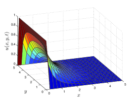
(b) $\lambda=1,~{}\nu=2$

Figure 1: Numerical solution profiles of velocity $u(x,y,t)$ at $~{}\alpha=0.8,~{}\beta=0.6.$

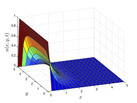
(a) $~{}\alpha=0.6,~{}\beta=0.5$

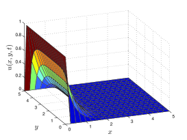
(b) $~{}\alpha=0.8,~{}\beta=0.2$

Figure 2: Numerical solution profiles of velocity $u(x,y,t)$ at $~{}\lambda=2,~{}\nu=1$.

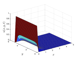
(a) $~{}t=0.5$

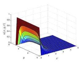
(b) $~{}t=1$

Figure 3: Numerical solution profiles of velocity $u(x,y,t)$ of at $~{}\alpha=0.8,~{}\beta=0.4,~{}\lambda=5,~{}\nu=2$.

7 Conclusion

In this paper, we proposed a finite difference method to solve the multi-term time fractional diffusion equation incorporating the unsteady MHD Couette flow of a generalized Oldroyd-B fluid. We give a implicit finite difference schemes with accuracy of $O(\tau^{\min\{3-\gamma_{l},2-\alpha_{m},2-\beta_{r}\}}+h_{x}^{2}+h_{y}^{2})$. In addition, we established the stability and convergence analysis for the implicit difference scheme. Two numerical examples were exhibited to verify the effectiveness and reliability of our method. We can conclude that our numerical method is robust and can be extended to other multi-term time fractional diffusion equations, such as the generalized Oldroyd-B fluid in a rotating system and the generalized Maxwell fluid model. In future work, we shall investigate alternating direction implicit (ADI) method to the two-dimensional generalized Oldroyd-B fluid, convert the two-dimensional computation to several one-dimensional ones, and reduce the computing time and storage.
Acknowledgements

The first author wishes to acknowledge that this work was partially supported by National Natural Science Foundation of China (Nos.11801060). The second two author wish to acknowledge that this research was partially supported by the Australian Research Council (ARC) via the Discovery Project (DP180103858).

References

• [1] R.L. Bagley, P.J. Torvik, A theorectical basis for the application of fractional calculus to viscoelasticity, Journal of Rheology, 27, 201-210 (1983)
• [2] C. Friedrich. Relaxation and retardation functions of the Maxwell model with fractional derivative, Rheologica Acta, 30, 151-158 (1991)
• [3] N. Makris, M.C. Constantinou, Fractional-derivative Maxwell model for viscous danmpers, Journal of Structural Engineering, 117, 2708-2724 (1991)
• [4] A. Hern$\acute{a}$ndez-Jimenez, J. Hern$\acute{a}$ndez-Santiago, A. Macisa-Garc$\acute{i}$a, J. S$\acute{a}$nchez-Gonz$\acute{a}$lez, Relaxation modulus in PMMA and PTFE fitting by fractional Maxwell model, Polymer Testing, 21, 325-331 (2002)
• [5] H.T. Qi, M. Y. Xu, Some unsteady unidirectional flows of a generalized Oldroyd-B fluid with fractional derivative, Appl. Math. Model., 33, 4184-4191 (2009)
• [6] J. Zhao, L. Zheng, Z. Zhang, F. Liu, Unsteady natural convection boundary layer heat transfer of fractional Maxwell viscoelastic fluid over a vertical plate, International Journal of Heat and Mass Transfer, 97, 760-766 (2016)
• [7] J. Zhao, L. Zheng, X.X. Zhang, F. Liu, X. Chen, Unsteady natural convection heat transfer past a vertical flat plate embedded in a porous medium saturated with fractional Qldroyd-B fluid, Journal of Heat Transfer, 139, 012501 (2017)
• [8] Y. Jiang, H. Qi, H. Xu, X. Jiang, Transient electroosmotic slip flow of fractional Oldroyd-B fluids, Microfluid Nanofluid, 21, 1-10 (2017)
• [9] G.M. Sutton, A. Sherman, Engineering magnetohydrodynamics, McGraw-Hill, New York (1965)
• [10] Y.Q. Liu, L.C. Zheng, X.X. Zhang, Unsteady MHD Couette flow of a generalized Oldroyd-B fluid with fractional derivative, Comput. Math. Appl., 61, 443-450 (2011)
• [11] L.C. Zheng, Y.Q. Liu, X.X. Zhang, Slip effects on MHD flow of a generalized Oldroyd-B fluid with fractional derivative, Nonlinear Analysis: Real World Applications, 13, 513-523 (2012)
• [12] M. Khan, T. Hayat, S. Asghar, Exact solution for MHD flow of a generalzied Oldroyd-B fluid with modified Darcy's law, Int. J. Eng. Sci., 44, 333-339 (2006)
• [13] M. Khan, K. Maqbool, T. Hayat, Influence of Hall current on the flows of a generalzied Oldroyd-B fluid in a porous space, Acta Mechanica, 184, 1-13 (2006)
• [14] Constantin Fetecaua, Corina Fetecau, M. Kamran, D. Vieru, Exact solutions for the flow of a generalized Oldroyd-B fluid induced by a constantly accelerating plate between side walls perpendicular to the plate, J. Non-Newtonian Fluid Mech. 156, 189201 (2009)
• [15] R. Hilfer, Applications of Fractional Calculus in Physics, World Scientifi Press, Singapore (2000)
• [16] I. Podlubny, Fractional differential equations, Academic Press, San Diego (1999)
• [17] C. Ming, F. Liu, L. Zheng, I. Turner, V. Anh, Analytical solutions of multi-term time fractional differential equations and application to unsteady flows of generalized viscoelastic fluid, Comput. Math. Appl., 72, 2084-2097 (2016)
• [18] X.Y. Jiang, H.T. Qi, Thermal wave model of bioheat transfer with modified Riemann-Liouville fractional derivative, J. Phys. A: Math. Theor., 45, 831-842 (2012)
• [19] F. Liu, V. Anh and I. Turner, Numerical solution of the space fractional Fokker-Planck Equation, Journal of Computational and Applied Mathematics, 166, 209-219 (2004)
• [20] F. Liu, P. Zhuang, V. Anh, I. Turner and K. Burrage , Stability and Convergence of the difference Methods for the space-time fractional advection-diffusion equation, Applied Mathematics and Computation, 191, 12-20 (2007)
• [21] P. Zhuang, F. Liu, V. Anh and I. Turner, New solution and analytical techniques of the implicit numerical methods for the anomalous sub-diffusion equation, SIAM J. Numer. Anal., 46, 1079-1095 (2008)
• [22] P. Zhuang, F. Liu, V. Anh and I. Turner, Numerical methods f or the variable-order fractional advection-diffusion with a nonlinear source term, SIAM J. Numer. Anal., 47, 1760-1781 (2009)
• [23] F. Liu, M.M. Meerschaert, R. McGough, P. Zhuang and Q. Liu, Numerical methods for solving the multi-term time fractional wave equations, Fractional Calculus & Applied Analysis, 16, 9-25 (2013)
• [24] F. Liu, P. Zhuang, I. Turner, V. Anh and K. Burrage, A semi-alternating direction method for a 2-D fractional FitzHugh-Nagumo monodomain model on an approximate irregular domain, J. Comp. Physics, 293, 252-263 (2015)
• [25] L.B. Feng, P. Zhuang, F. Liu, I. Turner, V. Anh, J. Li, A fast second order accurate method for a two-sided space-fractional diffusion equation with variable coefficients, Comput. Math. Appl., 73, 1155-1171(2017)
• [26] Y. Zhao, Y. Zhang, F. Liu, I. Turner, Y. Tang and V. Anh, Analytical solution and nonconforming finite element approximation for the 2D multi-term fractional subdiffusion equation, Applied Mathematical Modelling, 40, 8810-8825 (2016)
• [27] Z. Yang, Z. Yuan, Y. Nie, J. Wang, X. Zhu, F. Liu, Finite element method for nonlinear Riesz space fractional diffusion equations on irregular domains, J. Comp Physics, 330, 863-883 (2017)
• [28] Xuan Zhao, Xiaozhe Hu, Wei Cai, George Em Karniadakis, Adaptive finite element method for fractional differential equations using hierarchical matrices, Computer Methods in Applied Mechanics and Engineering, 325, 56-76 (2017)
• [29] Wenping Fan, Fawang Liu, A numerical method for solving the two-dimensional distributed order space-fractional diffusion equation on an irregular convex domain, Applied Mathematics Letter, 77, 114-121 (2018)
• [30] F. Liu, P. Zhuang, I. Turner, K. Burrage and V. Anh, A new fractional finite volume method for solving the fractional diffusion equation, Applied Mathematical Modelling, 38,3871-3878 (2014)
• [31] J. Li, F. Liu, L. B. Feng, I. Turner, A novel finite volume method for the Riesz space distributed-order advection-diffusion equation, Appl. Math. Model., 46, 536-553(2017)
• [32] F. Zeng, F. Liu, C. Li, K. Burrage, I. Turner, V.Anh, A Crank-Nicolson ADI spectral method for a two-dimensional Riesz space fractional nonlinear reaction-diffusion equation, SIAM J. Numer. Anal., 52, 2599-2622 (2014)
• [33] M. Zheng, F. Liu, I. Turner and V. Anh, A novel high order space-time spectral method for the time-fractional Fokker-Planck equation, SIAM J. Sci. Computing, 37, A701-A724 (2015)
• [34] X. Zhao and Z.M. Zhang, Superconvergence points of fractional spectral interpolation, SIAM J. SCI. Comput., 38, A598-A613 (2016)
• [35] Q. Liu, F. Liu, I. Turner , V. Anh and Y. Gu A RBF meshless approach for modeling a fractal mobile/immobile transport model, Appl. Math. Comp., 226, 336-147 (2014)
• [36] Q. Liu, F. Liu, Y. Gu , P. Zhuang, J. Chen, I. Turner, A meshless method based on Point Interpolation Method (PIM) for the space fractional diffusion equation, Appl. Math. Comp., 256, 930-938 (2015)
• [37] E. Bazhlekova, I. Bazhlekov, Viscoelastic flows with fractional derivative models: computational approach by convolutional calculus of Dimovski, Fract. Calc. Appl. Anal., 17, 954-976 (2014)
• [38] L.B. Feng, F. Liu, I. Turner, P.H. Zhuang, Numerical methods and analysis for simulating the flow of a generalized Oldroyd-B fluid between two infinite parallel rigid plates, International Journal of Heat and Mass Transfer, 115, 1309-1320 (2017)
• [39] A.A. Alikhanov, A new difference scheme for the time fractional diffusion equation, Journal of Computational Physics, 280, 424-438 (2015)
• [40] I. Karatay, N. Kale, S.R. Bayramoglu. A new difference scheme for time fractional heat equations based on the Crank-Nicholson method, Fractional Calculus and Applied analysis, 16, 892-910 (2013)
• [41] J.C. Liu, H. Li, Y. Liu, A new fully discrete finite difference/element approxiamation for fractional cable equation, J. Appl. Math. Comput., 52, 345-361 (2016)
• [42] J.C. Lopez-Marcos, A difference scheme for a nonlinear partial integrodifferential equation, SIAM Journal on Numerical Analysis, 27, 20-31 (1990)
• [43] F. Liu, P. Zhuang and Q. Liu, Numerical Methods of Fractional Partial Differential Equations and Applications, Science Press, China (in Chinese) (2015)