Predicting Stochastic Human Forward Reachable Sets Based on Learned Human Behavior

Abstract

With the recent surge of interest in introducing autonomous vehicles to the everyday lives of people, developing accurate and generalizable algorithms for predicting human behavior becomes highly crucial. Moreover, many of these emerging applications occur in a safety-critical context, making it even more urgent to develop good prediction models for human-operated vehicles. This is fundamentally a challenging task as humans are often noisy in their decision processes. Hamilton-Jacobi (HJ) reachability is a useful tool in control theory that provides safety guarantees for collision avoidance. In this paper, we first demonstrate how to incorporate information derived from HJ reachability into a machine learning problem which predicts human behavior in a simulated collision avoidance context, and show that this yields a higher prediction accuracy than learning without this information. Then we propose a framework to generate stochastic forward reachable sets that flexibly provides different safety probabilities and generalizes to novel scenarios. We demonstrate that we can construct stochastic reachable sets that can capture the trajectories with probability from $0.75$ to $1$.

I Introduction

In recent years, there has been much excitement in introducing intelligent systems that can navigate autonomously in environments with humans. For example, many self-driving car companies [1], [2], [3] have emerged in the past few years. Furthermore, projects like Amazon Prime Air [4] and Google’s Project Wing [5] aim to tap into the airspace for package delivery. There has also been immense interest in using UAVs for disaster response [6]. While roads provide structure, in airspace the interaction of vehicles occurs in a more unstructured setting, presenting the challenge of making predictions based on more limited information.

Critical to introducing autonomous vehicles into the workspace of humans is safety. The authors in [7] have focused on safety from a differential game perspective by characterizing the set of states from which one vehicle is guaranteed to be safe from a second assuming the second can take worst case actions within a bounded set. In [8], the authors demonstrate learning these bounds online in an uncertain environment. The authors in [9] characterize the notion of safety using torque limits on the robot. However, these works don’t consider the complexity of having humans in the environment. Taking humans into account is challenging because unlike dynamics model governing the robotic systems, we don’t generally have models for how humans make decisions in unstructured scenarios.

Key to having safe human-robot interaction is the ability for robots to navigate safely around human-operated vehicles. To enable this, the autonomous systems need to make predictions of human behaviors to avoid collisions. Past work has used various methods to perform behavior prediction of vehicles operated by humans. Many works have modeled humans as dynamical systems optimizing their own cost functions [10], [11]. Inverse reinforcement learning aims to learn these cost functions by observing past trajectories of the humans. There has also been work on using recurrent neural networks to make predictions on future trajectories [12], [13]. However, the methods presented in [10]-[13] only generate a single trajectory and do not provide probabilistic information of future trajectories. Since human behavior is noisy, having probabilistic information on future trajectories is important.

In the control theory literature, HJ reachability theory models the worst case scenario [7] and hence is often overly conservative when applied to real world scenarios. There has been a growing body of work in using stochastic reachable sets to reduce conservatism and model uncertainty. For example, [14] derives a stochastic reachable set and uses it for motion planning by making assumptions on the behavior of moving obstacles a priori. However, humans often don’t satisfy these assumptions and human behavior is also often influenced by the behavior of other vehicles in the environment.

In [15], the authors develop the notion of a human safe set for a human supervisor, to model when the supervisor would start to intervene with robot teams operating on their own in order to avoid static obstacles. However, this does not provide information on a mapping from any joint configuration of the human and robot to the human’s action when we aim to also model how the human would avoid, for example, predicting the direction of avoidance, and the entire avoidance process. In this paper, we also aim to model the situation in which humans are avoiding moving robots and comprehensively evaluate the effectiveness of incorporating varying degrees of information derived from HJ reachability.

In [16], the authors learn a forward reachable set by optimizing the disturbance bound, learning from data that is repeatedly gathered from similar initial configurations and generating a reachable set that satisfies an accuracy threshold. However, if we aim to apply the learned reachable set to a scenario in which the two vehicles are approaching from an angle different from what’s seen in the training data set, the reachable set generated will not be suitable. In [17], the authors assume that there are different modes that humans are in and learn a reachable set for each of these distinct modes. In this paper, we are interested in prediction methods that generalize to novel scenarios without the need to train a reachable set for each scenario.

In this paper, we first demonstrate how to incorporate information derived from HJ reachability in learning human behavior in a specific example of a simulated two vehicle unstructured setting. We illustrate that the use of HJ reachability yields considerable improvement in predicting human behavior when compared to not using it, for the humans that participated in our study. Furthermore, we propose a framework for learning stochastic human forward reachable sets (SHFRS) that flexibly captures regions with varying levels of safety. The proposed framework generalizes to prediction in scenarios not trained on. We validate our approaches on data gathered from human experiments with 8 participants.

The paper is organized as follows: section II presents the background of HJ reachability in the context of two vehicle collision avoidance. Section III presents our problem statement, how we incorporate information derived from HJ reachability into the learning problem, and the stochastic reachable set framework. Section IV presents our experiment setup, evaluation metrics, experimental results, and an implementation of the stochastic forward reachable set method described in III. Section V includes conclusion and future work. Due to space constraints, all proofs are omitted, but can be found in the full version of this paper on arXiv.

II Background

Our proposed method builds on HJ reachability theory [7]. HJ reachability is a control-theoretic method that provides safety certificates by characterizing the set of states that could, under the worst case behavior of the unknown but bounded disturbance, lead to danger.

We give a brief overview of how to apply HJ reachability to solve a pairwise collision avoidance problem such as the one in [7]. Consider two vehicles $Q_{1},Q_{2}$ described by the following ordinary differential equations (ODE):

$$\dot{x}_{i}=f_{i}(x_{i},u_{i}),\quad u_{i}\in\mathcal{U}_{i},\quad i=1,2.$$ (1)

Given the dynamics of the two vehicles (1), we can derive the relative dynamics in the form of (2):

$$\dot{x}_{ij} =g_{ij}(x_{ij},u_{i},u_{j})$$ (2)

$$u_{i} \in\mathcal{U}_{i},u_{j}\in\mathcal{U}_{j}\quad i,j=1,2,\quad i\neq j.$$

We assume the functions $f_{i}$ and $g_{ij}$ are uniformly continuous, bounded, and Lipschitz continuous in arguments $x_{i}$ and $x_{ij}$ respectively for fixed $u_{i}$ and $(u_{i},u_{j})$ respectively. In addition, the control functions $u_{i}(\cdot)\in\mathbb{U}_{i}$ are drawn from the set of measurable functions.

The set of states that represents a collision is denoted as $\mathcal{Z}_{ij}$, and we compute the following backward reachable set (BRS), which is the set of states from which a collision could occur over $[0,t]$ based on the worst case action of $Q_{j}$:

$$\mathcal{V}_{ij}(t)=\{x_{ij}:\forall u_{i}\in\mathbb{U}_{i},\exists u_{j}\in\mathbb{U}_{j},$$ (3)

$$x_{ij}(\cdot)\text{ satisfies \eqref{eq:rdyn}},\exists s\in[0,t],x_{ij}(s)\in\mathcal{Z}_{ij}\}.$$

Reachability theory is valid for any time horizon $t$; however, for clarity, we will let $t\rightarrow\infty$ in this paper. $\mathcal{V}_{ij}$ can be obtained as the sub-zero level set of the viscosity solution $V_{ij}(t,x)$ of a terminal value HJ PDE. For details on obtaining $V_{ij}$, please see [7]. The BRS can thus be denoted as $\mathcal{V}_{ij}=\{x_{ij}\in\mathbb{R}^{n}:\lim_{t\rightarrow\infty}V_{ij}(t,x_{ij})\leq 0\}$. We will also use a slight abuse of notation and write $V_{ij}(x_{ij})=\lim_{t\rightarrow\infty}V_{ij}(t,x_{ij})$. The interpretation is that $Q_{i}$ is guaranteed to be able to avoid collision with $Q_{j}$ over an infinite time horizon as long as the optimal control is applied as soon as the potential conflict occurs, represented by the sub-zero level set of $V_{ij}(x_{ij})$.

III Methodology

We aim to predict the behavior of a human controlling a vehicle (which we will call $Q_{\mathcal{H}}$ for human vehicle) in a shared space with an autonomous vehicle (called $Q_{\mathcal{R}}$ for robot vehicle), in an unstructured setting. The unstructured setting presents the challenge of using a limited amount of information to correctly model humans. The methodology section consists of two parts. In the first, we frame the learning problem and propose a way to use information derived from HJ reachability in making better predictions. In the second, we propose a framework to generate stochastic human forward reachable sets (SHFRS) using the behavior prediction obtained from the result of the learning problem in the first part, although the proposed framework can work with any learning model that outputs probabilistic prediction over actions of humans.

III-A Predicting human actions

III-A1 Problem Statement

In an environment with a human vehicle $Q_{\mathcal{H}}$ and a robot vehicle $Q_{\mathcal{R}}$ with dynamics in the form of (1), the human operator controls $Q_{\mathcal{H}}$ to avoid colliding with $Q_{\mathcal{R}}$. The human can provide control from a discrete set of $M$ control inputs $\{u_{1},\dots,u_{M}\}$ where $u_{min}\leq u_{m}\leq u_{max},m\in\{1,\dots,M\}$. For example, these could be one-dimensional real numbers corresponding to turning clockwise, turning counter-clockwise, or going straight. Let the states of the human and robot be denoted as $x_{\mathcal{H}}$ and $x_{\mathcal{R}}$ respectively. We aim to learn to predict the human action $\hat{u}$ within $\{u_{1},\dots,u_{M}\}$ at any joint configuration of $Q_{\mathcal{H}}$ and $Q_{\mathcal{R}}$. Our first contribution is to show through a set of human experiments that incorporating information derived from HJ reachability into the proposed learning problem can improve accuracy in prediction.

III-A2 Proposed method

In machine learning, feature vectors are representations of data points that can potentially improve the predictive performance. Since we’re working in an unstructured environment, we avoid direct dependency on absolute states and use the relative state $x_{\mathcal{H}\mathcal{R}}=x_{\mathcal{H}}-x_{\mathcal{R}}$.

The construction of good features is in general a challenging but important problem in machine learning [18]. In this project, we choose from a set of ”standard” geometric features, and augment with features derived from the safety value functions. The standard features we can incorporate are the translational and rotational components of the relative state. We also include cosine and sine of the rotational components in the relative states to provide nonlinear angular information. We denote features relevant to translation properties as $\vec{g}_{t}$, features relevant to rotational properties as $\vec{g}_{r}$, and features relevant to the trigonometric properties of the angles as $\vec{g}_{trig}$. For example, if the state of the vehicle is described by $x_{\mathcal{H}}=\begin{bmatrix}x_{\mathcal{H},1}&x_{\mathcal{H},2}&x_{\mathcal{H},3}\end{bmatrix}$ and $x_{\mathcal{R}}=\begin{bmatrix}x_{\mathcal{R},1}&x_{\mathcal{R},2}&x_{\mathcal{R},3}\end{bmatrix}$ where the first, second, and third components correspond to the $x$ coordinates, $y$ coordinates, and rotational angles, the relative state is $x_{\mathcal{H}\mathcal{R}}=\begin{bmatrix}x_{\mathcal{H}\mathcal{R},1}&x_{\mathcal{H}\mathcal{R},2}&x_{\mathcal{H}\mathcal{R},3}\end{bmatrix}=\begin{bmatrix}x_{\mathcal{H},1}-x_{\mathcal{R},1}&x_{\mathcal{H},2}-x_{\mathcal{R},2}&x_{\mathcal{H},3}-x_{\mathcal{R},3}\end{bmatrix}.$ Then based on our feature construction method, $\vec{g}_{t}\coloneqq\begin{bmatrix}\left|x_{\mathcal{H}\mathcal{R},1}\right|&\left|x_{\mathcal{H}\mathcal{R},2}\right|\end{bmatrix}^{T}$, $\vec{g}_{r}\coloneqq\begin{bmatrix}x_{\mathcal{H}\mathcal{R},3}\end{bmatrix}^{T}$, and $\vec{g}_{trig}\coloneqq\begin{bmatrix}cos\left(x_{\mathcal{H}\mathcal{R},3}\right)&sin\left(x_{\mathcal{H}\mathcal{R},3}\right)\end{bmatrix}^{T}$. Combining everything, we have that the standard feature vector has the form $\vec{g}_{std}\coloneqq\begin{bmatrix}\vec{g}_{t}^{T}&\vec{g}_{r}^{T}&\vec{g}_{trig}^{T}\end{bmatrix}^{T}.$

In safety critical scenarios, past works predominantly incorporate distance, measured by the l-2 norm, $\left\lVert\cdot\right\rVert_{2}$, of the translational properties in relative states, as a feature in learning human behavior. For example, using the previous example, the distance feature is $g_{d}\coloneqq\left\lVert\begin{bmatrix}x_{\mathcal{H}\mathcal{R},1}&x_{\mathcal{H}\mathcal{R},2}\end{bmatrix}\right\rVert_{2}$.

We hypothesize that safety levels derived from HJ reachability can potentially provide crucial information in predicting human action and the safety levels viewed from different agents may both provide valuable information. Let the safety levels of the human with respect to the robot be denoted as $V_{\mathcal{H}\mathcal{R}}(x_{\mathcal{H}\mathcal{R}})$ and the safety levels of the robot with respect to the human be denoted as $V_{\mathcal{R}\mathcal{H}}(x_{\mathcal{R}\mathcal{H}})$. If we include all the features proposed so far, we have the feature vector $\vec{g}=\begin{bmatrix}\vec{g}_{std}^{T}&g_{d}&V_{\mathcal{H}\mathcal{R}}(x_{\mathcal{H}\mathcal{R}})&V_{\mathcal{R}\mathcal{H}}(x_{\mathcal{R}\mathcal{H}})\end{bmatrix}^{T}.$

Now we present how we learn the human actions given the construction of feature vector $\vec{g}$. Let the data set be represented as $\{x_{\mathcal{H}\mathcal{R},n},u_{n}\}_{n=1}^{N}$, where $N$ represents the number of data points, $x_{\mathcal{H}\mathcal{R},n}$ represents the relative state of data point $n$, and $u_{n}$ represents the action the human took at this relative state. We call $u_{n}$ the label for datapoint $x_{\mathcal{H}\mathcal{R},n}$. Let $\vec{g}_{n}$ be the feature vector for $x_{\mathcal{H}\mathcal{R},n}$.

To model the problem probabilistically, we denote the probability of label $u_{n}$ of a datapoint $x_{\mathcal{H}\mathcal{R},n}$ as the function $P(u_{n}|x_{\mathcal{H}\mathcal{R},n};\theta)$ that is parameterized by $\theta$, with the goal to learn the parameter $\theta$. We assume that the data points are independent and identically distributed (iid) and we learn the parameter $\theta$ by maximizing the probability

$$\underset{\theta}{max}\text{ }\prod_{n=1}^{N}P(u_{n}|x_{\mathcal{H}\mathcal{R},n};\theta).$$ (4)

This is referred to as the maximum likelihood method. Here we refer to $P(u_{n}|x_{\mathcal{H}\mathcal{R},n};\theta)$ as the function approximator.

Alternatively, we could make no probabilistic assumption on the data. For example, a Support Vector Machine (SVM) finds a hyperplane that separates data points with different labels. Another example is a decision tree, which uses a tree-like structure to separate the data by recursively grouping it based on the decision rule at each node of the tree.

III-B A framework for generating stochastic human forward reachable sets (SHFRS) based on learned human behavior

III-B1 Problem statement

We aim to provide a framework to generate stochastic human forward reachable sets (SHFRS), with varying levels of safety, that capture future trajectories of $Q_{H}$. Mathematically, the problem is defined as follows: Let $T_{c}$ denote the current time step. Given the past and current states of the trajectory, $\{x_{\mathcal{H}}^{(i)},x_{\mathcal{R}}^{(i)}\}_{i=0}^{T_{c}}$, develop a framework to generate a SHFRS $\mathcal{S}$ composed of $F$ mutually disjoint regions $\mathcal{S}_{j}$ such that each region $\mathcal{S}_{j}$ is associated with a probability $p_{\mathcal{S}_{j}}$. Furthermore, the probabilities $p_{\mathcal{S}_{j}}$’s should satisfy $\sum_{j=1}^{F}p_{\mathcal{S}_{j}}=1.$

We say that a region provides a higher safety probability if the region captures future trajectories with a higher probability. Our second main contribution is thus a framework that provides varying levels of safety probabilities through stochastic reachable sets in novel scenarios.

III-B2 Proposed method

To generate a SHFRS satisfying the properties described earlier, we learn $F$ forward reachable sets, $\mathcal{F}_{1},\dots,\mathcal{F}_{F}$ that satisfy the following properties:

• $\mathcal{F}_{1}\subseteq\mathcal{F}_{2}\subseteq\dots\subseteq\mathcal{F}_{F-1}\subseteq\mathcal{F}_{F}$.

• We associate a probability $p_{\mathcal{F}_{j}}$ with each reachable set $\mathcal{F}_{j}$. This probability specifies the likelihood that the trajectory in the next $T$ time steps will be within $\mathcal{F}_{j}$. $p_{\mathcal{F}_{1}},\dots,p_{\mathcal{F}_{F}}$ should satisfy $p_{\mathcal{F}_{1}}\geq\underline{p}$, $p_{\mathcal{F}_{F}}=1$, and $p_{\mathcal{F}_{j+1}}\geq p_{\mathcal{F}_{j}},\forall j\in\{1,\dots,F-1\}$. Note that $\underline{p}$ represents the desired minimum probability with which the smallest reachable set $\mathcal{F}_{1}$ should capture the human trajectories.

Note that we define $\mathcal{F}_{0}=\emptyset$. With this definition , $p_{\mathcal{F}_{0}}=0$. The set of constraints $p_{\mathcal{F}_{j+1}}\geq p_{\mathcal{F}_{j}},\forall j\in\{1,\dots,F-1\}$ encourages the set of reachable sets to provide increasing levels of safety. The constraint $p_{\mathcal{F}_{F}}=1$ enables us to provide a safety certificate in the worst case scenario.

We propose to generate these reachable sets $\mathcal{F}_{j}$’s by learning time-varying control input bounds for each. For simplicity, we consider the case in which the human input is one dimensional, though our method generalizes to the multi-dimensional case.

Definition 1

Time-varying bounds on control inputs: Let $\underline{u}_{j}^{(i)}$ and $\boldmath\bar{u}_{j}^{(i)}$ denote the lower and upper bounds on the control inputs for reachable set $\mathcal{F}_{j}$, between time $t_{T_{c}+i}$ and $t_{T_{c}+i+1}$. This is defined for all $\forall i\in\{0,\dots,T-1\}$, $\forall j\in\{1,\dots,F\}$. Note that $t_{T_{c}+i}$ corresponds to the real-valued time at time step $T_{c}+i$.

Given $\underline{u}_{j}^{(i)}$ and $\bar{u}_{j}^{(i)}$ for all $i\in\{0,\dots,T-1\}$, we can construct the forward reachable set $\mathcal{F}_{j}$ using the following definition.

Definition 2

Forward reachable set with time-varying constraints on inputs: Suppose we have time varying constraints for the control inputs, i.e., there exists $t_{0},\dots,t_{T}$ such that $0=t_{0}<t_{1}<\dots<t_{T-1}<t_{T}$ and the control input between time $t_{i}$ and time $t_{i+1}$ is within the set $U^{(i)}=[\underline{u}_{j}^{(i)},\bar{u}_{j}^{(i)}]$. Denote $\mathcal{L}$ as the initial set of states to grow the reachable set from. To make this well defined on the boundary time points, we define the reachable set to be $\mathcal{F}(t_{0})=\mathcal{L}$, $\mathcal{F}(t_{i+1})=\{x:\exists u(t)\in U^{(i)}\text{ s.t. }t\in[t_{i},t_{i+1}],x(\cdot)\text{ satisfies }\dot{x}=f(x,u),x(t_{i})\in\mathcal{F}(t_{i}),x(t)=x\}.$

Algorithm 1 presents how we determine the time-varying bounds $\underline{u}_{j}^{(i)},\bar{u}_{j}^{(i)}$. The algorithm takes in the following arguments: $\{x^{(i)}\}_{i=0}^{T_{c}}$, $G$, $\{\epsilon_{j}\}_{j=1}^{F}$, and $\{k^{(i)}\}_{i=0}^{T-1}$. We use $x^{(i)}$ as a shorthand notation for $(x_{\mathcal{H}}^{(i)},x_{\mathcal{R}}^{(i)})$. For generality, the algorithm takes in joint states from all past time steps and the current time step $T_{c}$. The argument $G$ represents any learned function that can take in the past and current joint configurations of the vehicles, and outputs a probabilistic distribution over the set of possible actions. Note that we allow $G$ to take in the past states for prediction here, however, it could also be the case that $G$ makes predictions solely based on the current joint configuration like the function approximators learned in III-A. As we illustrate in the next paragraph as we describe our Algorithm, the scalar $\epsilon_{j}$ determines how much to grow the input bounds for $\mathcal{F}_{j}$, and the positive integer $k^{(i)}$ indicates the number of likely actions we use to generate these bounds at time step $i$.

Algorithm 1, which learns time varying bounds for the human inputs, is described below. On line 1, ”low” and ”high” predicted joint states are initialized with the values of the current joint states; here $\hat{x}_{l}^{(T_{c}+i)},i>0,$ refers to the predicted joint states at time step $T_{c}+i$, using the low control input value, the subscript $h$ is used for the high control input value. Inside the loop, lines 3-4 obtain the $k^{(i)}$ top likely actions based on the learned function $G$, for both the low and high cases; and lines 5-6 obtain the corresponding lowest and highest value inputs, denoted $\underline{u}^{(i)},\bar{u}^{(i)}$ respectively. In lines 7-10, we obtain the corresponding desired $\underline{u}_{j}^{(i)},\bar{u}_{j}^{(i)}$ for each reachable set $\mathcal{F}_{j}$ by expanding $\underline{u}^{(i)},\bar{u}^{(i)}$ with $\epsilon_{j}$ as shown. Lines 11-12 obtain the robot’s actions for both the $l$ and $h$ cases using the function getRobotAction, which is defined using the robot’s model. On line 13, the predicted actions of the human for the case $l$ and $h$ at time step $T_{c}+i$ are set to be the lower and upper bounds, respectively, of the control input for the smallest reachable set $\mathcal{F}_{1}$. Lines 14-18 simulate the predicted states of the human and robot for the next time step $T_{c}+i+1$. This process repeats as $i$ increments.

input :  $\{x\}_{i=0}^{T_{c}}$, $G$, $\{\epsilon_{j}\}_{j=1}^{F}$, $\{k^{(i)}\}_{i=0}^{T-1}$

output :  $\underline{u}_{j}^{(i)},\bar{u}_{j}^{(i)}$ for $i\in\{0,\dots,T_{c}-1\}$, $j\in\{1,\dots,F\}$

1

2Assign $\hat{x}_{l}^{(T_{c})}=x^{(T_{c})}$, $\hat{x}_{h}^{(T_{c})}=x^{(T_{c})}$;

3 for $i\leftarrow 0$ to $T-1$ do

4       $\text{set\_}\hat{u}_{\mathcal{H},l}$ = getTopKPredictedHumanActions(G, $\{x\}_{i=0}^{T_{c}-1}$, $\{\hat{x}_{l}\}_{i=T_{c}}^{T_{c}+i}$, $k^{(i)}$ ) ;

5      

6      $\text{set\_}\hat{u}_{\mathcal{H},h}$ = getTopKPredictedHumanActions(G, $\{x\}_{i=0}^{T_{c}-1}$, $\{\hat{x}_{h}\}_{i=T_{c}}^{T_{c}+i}$, $k^{(i)}$ ) ;

7      

8      $\underline{u}^{(i)}=\text{ getMin }\left(\text{set\_}\hat{u}_{\mathcal{H},l},\text{set\_}\hat{u}_{\mathcal{H},h}\right)$ ;

9      

10      $\bar{u}^{(i)}=\text{ getMax }\left(\text{set\_}\hat{u}_{\mathcal{H},l},\text{set\_}\hat{u}_{\mathcal{H},h}\right)$ ;

11      

12      for $j\leftarrow 1$ to $F$ do

13             $\underline{u}_{j}^{(i)}=\operatorname{max}(\underline{u}^{(i)}-\epsilon_{j},u_{min})$ ;

14             $\bar{u}_{j}^{(i)}=\operatorname{min}(\bar{u}^{(i)}+\epsilon_{j},u_{max})$ ;

15            

16       end for

17      

18      $\hat{u}_{\mathcal{R},l}^{(T_{c}+i)}$ = getRobotAction( $\{x\}_{i=0}^{T_{c}-1}$, $\{\hat{x}_{l}\}_{i=T_{c}}^{T_{c}+i}$ ) ;

19      

20      $\hat{u}_{\mathcal{R},h}^{(T_{c}+i)}$ = getRobotAction( $\{x\}_{i=0}^{T_{c}-1}$, $\{\hat{x}_{h}\}_{i=T_{c}}^{T_{c}+i}$ );

21      

22      $\hat{u}_{\mathcal{H},l}^{(T_{c}+i)},\hat{u}_{\mathcal{H},h}^{(T_{c}+i)}=\underline{u}_{1}^{(i)},\bar{u}_{1}^{(i)}$ ;

23      

24      for boundType $\in\{l,h\}$ do

25             for agentType $\in\{\mathcal{H},\mathcal{R}\}$ do

26                   $\hat{x}_{\text{agentType,boundType}}^{(T_{c}+i+1)}=$ForwardDynamics(  $\hat{x}_{\text{agentType,boundType}}^{(T_{c}+i)},\hat{u}_{\text{agentType,boundType}}^{(i)})$ ;

27                  

28             end for

29            

30       end for

31      

32 end for

Algorithm 1 Generation of time-varying input bounds for reachable sets $\mathcal{F}_{j}$’s

We now present the conditions $\epsilon_{j}$’s should satisfy to enable $\mathcal{F}_{j}\subseteq\mathcal{F}_{j+1},\forall j\in\{1,\dots,F-1\}$.

Theorem 1

Based on this reachable set generation scheme, If for any $j\in\{1,\dots,F-1\}$, $\epsilon_{j}\leq\epsilon_{j+1}$ and $\forall j\in\{1,\dots,F\},\epsilon_{j}\geq 0$, for any $j\in\{1,\dots,F-1\}$, $\mathcal{F}_{j}\subseteq\mathcal{F}_{j+1}$.

We compute $p_{j}$ associated with $\mathcal{F}_{j}$ by letting it be the percentage of the human trajectories that fall entirely within the predicted $\mathcal{F}_{j}$.

Corollary 1

Using our algorithm, $p_{\mathcal{F}_{j+1}}\geq p_{\mathcal{F}_{j}},\forall j\in\{1,\dots,F-1\}.$

Corollary 2

If we set $\epsilon_{F}$ such that $\underline{u}_{F}^{(i)}=u_{min},\bar{u}_{F}^{(i)}=u_{max},\forall i\in\{0,\dots,T-1\}$, then $p_{\mathcal{F}_{F}}=1$.

Having $\sum_{j=1}^{F}p_{\mathcal{S}_{j}}=p_{\mathcal{F}_{F}}=1$ allows us to capture all possible future trajectories and provides us with the ability to use $\mathcal{F}_{F}$ as the most conservative safety standard.

IV Experiments

We conduct experiments to understand how incorporating information derived from HJ reachability affects the prediction of human behavior with our proposed method. Furthermore, we present the learned stochastic human forward reachable sets (SHFRS) generated based on our proposed framework with the same experimental data.

IV-A Experimental design

We recruited 8 participants between the age 20-27 from the university campus to participate in the experiment. We gather trajectory data by having each human subject control a human vehicle in a simulated environment with another robot vehicle. The robot vehicle has a goal which is displayed to the human, and the robot is automatically controlled to reach its designated goal in exactly 10 seconds. The human subject is informed that the robot is heading straight to the goal and will not actively avoid the human vehicle.

In our experiment, we use vehicles with the following dynamics:

$$\dot{p}_{x,i} =v\cos\psi_{i}$$ (5)

$$\dot{p}_{y,i} =v\sin\psi_{i}$$

$$\dot{\psi}_{i} =\omega_{i},\quad\omega_{min}\leq\omega_{i}\leq\omega_{max}$$

where the state variables $p_{x,i},p_{x,i},\psi_{i}$ represent the $x$ position, $y$ position, and heading of vehicle $Q_{i}$, $i\in\{\mathcal{H},\mathcal{R}\}$. Each vehicle travels at a constant speed of $v=2$, and its turn rate $\omega_{i}$ is constrained by $\omega_{min}=-0.5,\omega_{max}=0.5$. Using a computer keyboard, the participants can provide control inputs corresponding to $\{\omega_{min},0,\omega_{max}\}$, which are control inputs for turning right, going straight, and turning left respectively. We think that these controls are sufficient for the human participants to avoid the robot vehicle while not burdening the cognitive load of the humans by giving them an abundance of possible controls, which may confound the experimental results.

Two example scenes from our data collection web application are presented in the top two plots in Figure 1. The robot and human vehicle are colored in red and blue respectively. The tails and the directions of the arrows indicate the exact locations and orientations of the vehicles respectively. The goal of the robot is presented as a red square. The human operator is asked to provide control inputs so that the human vehicle avoids the danger zone of the robot vehicle, represented as $\mathcal{L}_{ij}=\{p_{x,ij}:(p_{x,i}-p_{x,j})^{2}+(p_{y,i}-p_{y,j})^{2}\leq R_{c}^{2}\}$, where $R_{c}=3$ in our experiment. Each scene is also designed so that if the human subject doesn’t avoid the robot, the human and robot vehicles will collide eventually. Hence the human subjects are instructed to continuously provide control inputs for avoidance starting from when they feel danger until they no longer think that the human vehicle and the robot vehicle will collide if they don’t provide any more avoidance inputs. The human does not need to repeatedly press the key to avoid but can just hold down the key to avoid continuously. The scene ends when the robot reaches the goal.

The experiment is divided into three phases. In the first phase, we provide instructions and the participants are given 1 minute to familiarize themselves with the interface we developed and the dynamics of the vehicle. In the second phase, participants are given three practice scenes to further familiarize themselves with the setup of the study. In the third phase, participants are given 50 vehicle avoidance tasks. The initial states of the human and robot vehicles are randomized for each scene. We record the states of the human and robot vehicles, along with the action of the human, every 0.2 seconds.

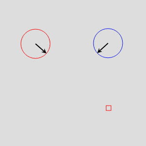
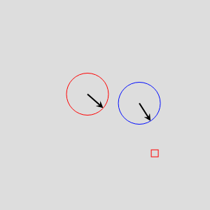
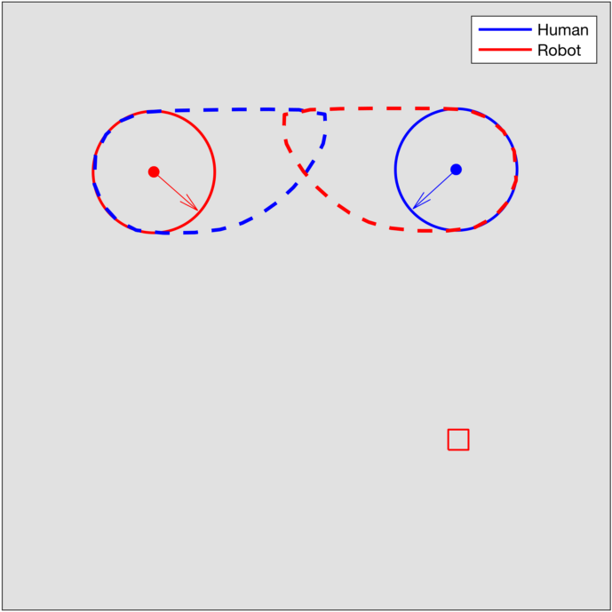
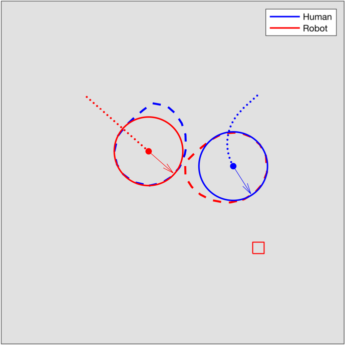
Figure 1: The top two figures illustrate the interface we designed to collect data from participants. The top left figure shows the initial configuration and the top right figure shows the configuration after the human has inputted controls to avoid the robot. The bottom figures illustrate the sub-zero level set for the value functions $V_{\mathcal{H}\mathcal{R}}$ and $V_{\mathcal{R}\mathcal{H}}$ for the configurations in the top figures, computed using [19]. Neither of the safety value functions are provided to the human subjects during the experiment: the subjects only see the scenes in the top figures.

IV-B Analysis of prediction performance

In this section, we present the experimental results of incorporating information derived from HJ reachability into the learning problem.

We perform a five fold cross validation to tune the hyperparameters of the models and evaluate the result based on predictive performance on the test data. We model that each human has a different pattern in avoidance behavior, hence, we trained a classifier for each subject. We perform an extensive comparison of incorporating different subsets of information derived from HJ reachability. To rigorously compare the sets of features, we conduct statistical significance tests to see if the differences in performance are statistically significant. We apply the Mann-Whitney test on pairs of feature sets and compute the p-values.

As described in III-A, the standard features are $\mathcal{B}=\{\left|p_{x,\mathcal{H}\mathcal{R}}\right|,\left|p_{y,\mathcal{H}\mathcal{R}}\right|,\psi_{\mathcal{H}\mathcal{R}},\cos\psi_{\mathcal{H}\mathcal{R}},\sin\psi_{\mathcal{H}\mathcal{R}}\}$. We augment these with features, $d_{\mathcal{H}\mathcal{R}}=\sqrt{p_{x,\mathcal{H}\mathcal{R}}^{2}+p_{y,\mathcal{H}\mathcal{R}}^{2}}$, $v_{\mathcal{R}}=V_{\mathcal{H}\mathcal{R}}(x_{\mathcal{H}\mathcal{R}})$, and $v_{\mathcal{H}}=V_{\mathcal{R}\mathcal{H}}(x_{\mathcal{R}\mathcal{H}})$ to the feature set, which represent the distance between the two vehicles, and the safety levels of the human relative to robot and robot relative to human, respectively. To obtain safety levels, we compute the BRS (3) with the relative dynamics of the two vehicles derived from the vehicle dynamics (5). To describe the sets of features, we use subscripts $d$, $h$, and $r$ to represent the addition of the features to the standard feature set $d_{\mathcal{H}\mathcal{R}}$, $v_{\mathcal{R}}$, and $v_{\mathcal{H}}$ respectively. For example, $\mathcal{B}_{hrd}=\mathcal{B}\cup\{v_{\mathcal{R}},v_{\mathcal{H}},d_{\mathcal{H}\mathcal{R}}\}$ and $\mathcal{B}_{hr}=\mathcal{B}\cup\{v_{\mathcal{H}},d_{\mathcal{H}\mathcal{R}}\}$.

We conduct two sets of experiments: in experiment (I), we perform prediction on the exact control the human inputs, i.e., we predict the control as one of the three possible control inputs, $\{\omega_{min},0,\omega_{max}\}$. In experiment (II), the goal is to predict whether the human will input control to avoid at any joint state of the $Q_{\mathcal{H}}$ and $Q_{\mathcal{R}}$, which is equivalent to predicting whether the input is $\omega=0$ or if the input falls in $\{\omega_{min},\omega_{max}\}$ in our setup. We consider the following metric for both sets of experiments:

• Accuracy: $\frac{1}{\sum_{k=1}^{K}L_{k}}\sum_{k=1}^{K}\sum_{l=1}^{L_{k}}\mathds{1}\{\hat{y}_{k}^{(l)}=y_{k}^{(l)}\}\times 100\%$ where $\hat{y}_{k}^{(l)}$ and $y_{k}^{(l)}$ represent the predicted action and the ground truth action of the human at time step $l$ in trajectory $k$ respectively. Here $K$ represents the number of trajectories and $L_{k}$ represents the number of time steps in trajectory $k$.

For experiment II, we further evaluate the following metrics:

• $D_{start}$: Let $\hat{T}_{k,f}$ be the first time step in trajectory $k$ that our algorithm predicts the vehicle avoids and $T_{k,f}$ be the first time step the human avoids in the experiment. This metric is defined as: $\frac{1}{K}\sum_{k=1}^{K}\left|\hat{T}_{k,f}-T_{k,f}\right|$.

• $D_{end}$: Let $\hat{T}_{k,e}$ be the last time step in trajectory $k$ that our algorithm predicts the vehicle avoids and $T_{k,e}$ be the last time step the human avoids in the experiment. This metric is defined as: $\frac{1}{K}\sum_{k=1}^{K}\left|\hat{T}_{k,e}-T_{k,e}\right|$.

We consider support vector machine (SVM), decision tree (DT), and logistic regression (LR) machine learning models. SVM and DT models don’t make assumptions about the probabilistic distribution of the data. LR assumes that each data point is iid. Despite the fact that the data we gather are temporally correlated, we are interested in investigating how well LR performs on the data.

Our experimental results indicate that incorporating the safety levels derived from HJ reachability can yield considerable improvement in predictive performance. Table I illustrates the accuracies obtained by applying the SVM, DT, and LR models on the two sets of experiments, (I) and (II). We can see that for all models on both tasks, using the feature set $\mathcal{B}_{hrd}$ yields the highest performance, considerably higher than just incorporating distance, $\mathcal{B}_{d}$ ($p<0.05$). It is also notable that for all three algorithms on both tasks, incorporating exactly one of the two safety levels $v_{\mathcal{H}},v_{\mathcal{R}}$ outperforms incorporating just the distance $d_{\mathcal{H}\mathcal{R}}$ ($p<0.05$). We see that incorporating the robot’s safety level with respect to the human, $v_{\mathcal{R}}$, generally, but not always, yields higher performance than if not including it. This suggests that taking into account the safety from the perspective of the robot vehicle is also important. With the feature set and model fixed, the accuracies in experiment (II) is in general higher than those in experiment (I). This is expected as in experiment (II), we need to also predict the direction of the avoidance. However, the difference is not big, suggesting that the algorithms did reasonably well in predicting avoidance direction.

Table II illustrates the performance of the models on predicting the first and last time steps of avoidance. We can see from the table that using DT with feature set $\mathcal{B}_{hrd}$ yields the best performance in metric $D_{s}$ and is on average $1.48$ time steps off from the ground truth, which is equivalent to $1.48\times 0.2=0.296$ seconds off since every time step is $0.2$ second apart. Similar to the accuracy metric, incorporating just one of the safety levels yields a more accurate prediction than just considering $d_{\mathcal{H}\mathcal{R}}$ ($p<0.05$). We can also see that including the feature $v_{\mathcal{R}}$ generally result in better prediction than including the feature $v_{\mathcal{H}}$. It is also interesting to see that the models did a much better job predicting when a human would start avoiding than when a human would end avoiding. We hypothesize that this is because humans are generally more noisy in determining when to stop avoiding after there is no longer immediate danger as once the danger is cleared, when to stop avoiding is less important.

	$\mathcal{B}_{hrd}$	$\mathcal{B}_{hr}$	$\mathcal{B}_{hd}$	$\mathcal{B}_{rd}$	$\mathcal{B}_{h}$	$\mathcal{B}_{r}$	$\mathcal{B}_{d}$
SVM (I)	78.67	78.46	76.56	76.74	75.11	76.33	69.75
DT (I)	75.77	74.24	73.65	75.27	71.37	73.65	68.68
LR (I)	77.73	77.4	74.71	77.38	73.31	76.61	69.15
SVM (II)	83.89	83.15	81.12	82.85	79.62	82.15	70.72
DT (II)	81.29	78.58	79.26	80.55	79.15	78.5	68
LR (II)	81.70	81.61	78.79	81.62	77.54	80.88	71.35

TABLE I: This table shows the accuracies of SVM, DT, and LR models using different feature sets. We can see that including the information derived from HJ reachability yields improvement in predictive performance than just including distance as a feature.

	$\mathcal{B}_{hrd}$	$\mathcal{B}_{hr}$	$\mathcal{B}_{hd}$	$\mathcal{B}_{rd}$	$\mathcal{B}_{h}$	$\mathcal{B}_{r}$	$\mathcal{B}_{d}$
SVM, $D_{s}$	2.02	2.06	2.23	1.88	2.3	2.03	4.22
DT, $D_{s}$	1.48	2.02	1.98	1.56	2.44	1.68	2.92
LR, $D_{s}$	2.43	2.84	2.6	2.29	2.93	2.83	7.3
SVM, $D_{e}$	6.7	7.38	8.67	7.03	8.78	8.07	15.94
DT, $D_{e}$	8.77	9.09	8.43	8.02	9.45	9.25	14.5
LR, $D_{e}$	7.67	7.35	9.17	7.72	9.96	8.09	17.57

TABLE II: This table shows results for the metrics $D_{start}$ ($D_{s}$) and $D_{end}$ ($D_{e}$). Similarly to the accuracy metric, we see that both safety levels derived from HJ reachability improve prediction performance.

Intuitively, we think the higher performance of including safety levels derived from HJ reachability is that inherently the safety levels encode some information about the dynamics and how dangerous the configuration is based on worst case analysis. The geometric distance of the two vehicles can also encode useful information about how dangerous the configuration might be, however, it’s not as informative as the safety levels.

IV-C Stochastic human forward reachable set (SHFRS) implementation

In this section, we demonstrate an implementation of our proposed forward reachable set prediction framework in III-B by applying our framework on the experimental data gathered. For demonstration purpose, we use the logistic regression predictor learned in experiment I in IV-B for prediction, although it is possible to use any predictor that gives probabilistic information on the predicted actions. Note that the constraint $p_{\mathcal{F}_{1}}\geq\underline{p}$ can always be satisfied by tuning $\epsilon_{1}$’s and $k^{(i)}$’s. The intuition is that the better the predictor we use in Algorithm I, the smaller $\epsilon_{1}$ and $k^{(i)}$’s are needed to achieve $p_{\mathcal{F}_{1}}\geq\underline{p}$. An example of the SHFRS using an implementation of this framework is illustrated in Figure 2. We can see that the stochastic reachable set we produce gives varying degrees of safety probabilities.

To provide intuition on the effect of tuning $\epsilon_{j}$’s and $k^{(i)}$’s during the optimization, we demonstrate the effect of changing these parameters. The leftmost figure of Figure 2 shows the stochastic reachable set generated with $\epsilon_{1}=0,\epsilon_{2}=0.15,\epsilon_{3}=0.25,\epsilon_{4}=0.4,\epsilon_{5}=1.0$ and $k^{(i)}=2,i\in\{0,1\}$ and $k^{(i)}=1,i\in\{2,\dots,9\}$. The SHFRS in the middle figure is generated by fixing the $k^{(i)}$’s used in the left figure and varying the $\epsilon_{j}$’s. We let $\epsilon_{1}=0.2$ $\epsilon_{2}=0.3,\epsilon_{3}=0.35,\epsilon_{4}=0.45$ and leave $\epsilon_{5}$ unchanged. Increasing $\epsilon_{j}$ makes the region $\mathcal{F}_{j}$ larger. On the other hand, the SHFRS in rightmost figure is generated by fixing the $\epsilon_{j}$’s used in generating the SHFRS in the leftmost figure and varying the $k^{(i)}$’s. We let $k^{(i)}=2,i=\{0\}$ and $k^{(i)}=1,i\in\{1,\dots,9\}$ in the rightmost figure. Making $k^{(i)}$ smaller decreases the area of $\mathcal{F}_{j}$’s, except for $\mathcal{F}_{F}$, which aims to capture the worst case scenario.

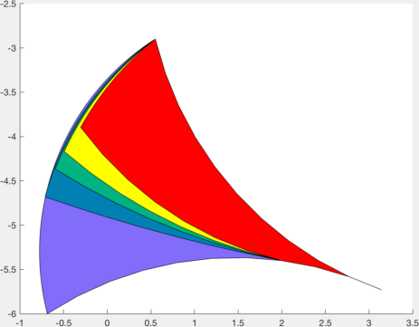
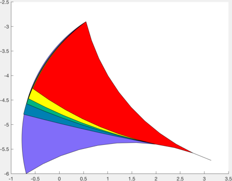
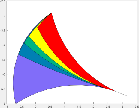
Figure 2: These are stochastic human forward reachable sets (SHFRS) generated using our framework. The algorithm predicts that the human will likely turn right within the next $T=10$ time steps. The regions in red, yellow, green, blue, purple correspond to $\mathcal{S}_{1},\mathcal{S}_{2},\mathcal{S}_{3},\mathcal{S}_{4},\mathcal{S}_{5}$ respectively. The middle figure is generated with the same $k^{(i)}$’s as the leftmost figure but the $\epsilon_{j}$’s used are larger or equal to those used in the leftmost figure. Increasing $\epsilon_{j}$ increases the area of $\mathcal{F}_{j}$. The rightmost figure is generated with the same $\epsilon_{j}$’s as the leftmost figure, but with $k^{(i)}$’s smaller or equal to those in the leftmost figure. We can see that decreasing $k^{(i)}$’s makes the areas of $\mathcal{F}_{j}$’s smaller. For the SHFRS in the middle figure, the probability for each of the five regions is: $p_{\mathcal{F}_{1}}=p_{\mathcal{S}_{1}}=0.752,p_{\mathcal{F}_{2}}=p_{\mathcal{S}_{1}\cup\mathcal{S}_{2}}=0.771,p_{\mathcal{F}_{3}}=p_{\cup_{i=1}^{3}\mathcal{S}_{i}}=0.773,p_{\mathcal{F}_{4}}=p_{\cup_{i=1}^{4}\mathcal{S}_{i}}=0.775,p_{\mathcal{F}_{5}}=p_{\cup_{i=1}^{5}\mathcal{S}_{i}}=1.0$.

Algorithm 1 can be computed efficiently online. The generation of SHFRS based on the output of Algorithm 1 can be computed online if the mapping from any $\{[\underline{u}_{j}^{(i)},\bar{u}_{j}^{(i)}]\}_{i=0}^{T-1}$ to $\mathcal{F}_{j}$ has been computed offline.

V Conclusion and Future Work

We first demonstrate how to incorporate information derived from HJ reachability into a machine learning problem and show that this can yield considerable improvement in prediction performance of human behavior compared with using one of the most typical features, the distance feature, in safety critical scenarios. We then propose a framework to generate stochastic human forward reachable set (SHFRS) that flexibly offers different levels of safety probabilities and generalizes to unseen scenarios. In future work, it would be interesting to develop methodologies to evaluate how useful safety levels from HJ reachability are for continuous action prediction or under situations where temporal information are considered. Other directions include further imposing metrics on the SHFRS framework and generalizing the framework to work with continuous action prediction.

VI Acknowledgement

The author would like to thank Prof. Claire Tomlin for providing advice on the project and helping to edit many parts of the paper.

References

- [1] Waymo, Inc. (2018) Waymo. [Online]. Available: https://waymo.com/
- [2] Cruise Automation, Inc. (2018) Cruise. [Online]. Available: https://getcruise.com/
- [3] Aurora, Inc. (2018) Aurora. [Online]. Available: https://aurora.tech/
- [4] Amazon.com, Inc. (2016) Amazon prime air. [Online]. Available: http://www.amazon.com/b?node=8037720011
- [5] Business Insider. (2017) Google’s drone delivery project just shared some big news about its future. [Online]. Available: https://www.businessinsider.com/project-wing-update-future-google-drone-delivery-project-2017-6
- [6] AUVSI News. (2016) Uas aid in south carolina tornado investigation. [Online]. Available: http://www.auvsi.org/blogs/auvsi-news/2016/01/29/tornado
- [7] I. Mitchell, A. Bayen, and C. Tomlin, “A time-dependent Hamilton-Jacobi formulation of reachable sets for continuous dynamic games,” IEEE Transactions on Automatic Control, vol. 50, no. 7, pp. 947–957, 2005.
- [8] A. K. Akametalu, J. F. Fisac, J. H. Gillula, S. Kaynama, M. N. Zeilinger, and C. J. Tomlin, “Reachability-based safe learning with gaussian processes,” in 53rd IEEE Conference on Decision and Control, Dec 2014, pp. 1424–1431.
- [9] D. Held, Z. McCarthy, M. Zhang, F. Shentu, and P. Abbeel, “Probabilistically safe policy transfer,” in 2017 IEEE International Conference on Robotics and Automation, ICRA 2017, Singapore, Singapore, May 29 - June 3, 2017, 2017, pp. 5798–5805.
- [10] P. Abbeel and A. Y. Ng, “Apprenticeship learning via inverse reinforcement learning,” in Proceedings of the Twenty-first International Conference on Machine Learning, ser. ICML ’04. New York, NY, USA: ACM, 2004.
- [11] B. D. Ziebart, A. L. Maas, J. A. Bagnell, and A. K. Dey, “Maximum entropy inverse reinforcement learning,” in Proceedings of the Twenty-Third AAAI Conference on Artificial Intelligence, AAAI 2008, Chicago, Illinois, USA, July 13-17, 2008, 2008, pp. 1433–1438. [Online]. Available: http://www.aaai.org/Library/AAAI/2008/aaai08-227.php
- [12] H. Wu, Z. Chen, W. Sun, B. Zheng, and W. Wang, “Modeling trajectories with recurrent neural networks,” in Proceedings of the Twenty-Sixth International Joint Conference on Artificial Intelligence, IJCAI-17, 2017, pp. 3083–3090. [Online]. Available: https://doi.org/10.24963/ijcai.2017/430
- [13] A. Alahi, K. Goel, V. Ramanathan, A. Robicquet, L. Fei-Fei, and S. Savarese, “Social lstm: Human trajectory prediction in crowded spaces,” in 2016 IEEE Conference on Computer Vision and Pattern Recognition (CVPR), June 2016, pp. 961–971.
- [14] N. Malone, K. Lesser, M. Oishi, and L. Tapia, “Stochastic reachability based motion planning for multiple moving obstacle avoidance,” in Proceedings of the 17th International Conference on Hybrid Systems: Computation and Control, ser. HSCC ’14. New York, NY, USA: ACM, 2014, pp. 51–60. [Online]. Available: http://doi.acm.org/10.1145/2562059.2562127
- [15] D. L. McPherson, D. R. R. Scobee, J. Menke, A. Y. Yang, and S. S. Sastry, “Modeling supervisor safe sets for improving collaboration in human-robot teams,” CoRR, vol. abs/1805.03328, 2018. [Online]. Available: http://arxiv.org/abs/1805.03328
- [16] V. Govindarajan, K. Driggs-Campbell, and R. Bajcsy, “Data-driven reachability analysis for human-in-the-loop systems,” in 2017 IEEE 56th Annual Conference on Decision and Control (CDC), Dec 2017, pp. 2617–2622.
- [17] K. R. Driggs-Campbell, R. Dong, and R. Bajcsy, “Robust, informative human-in-the-loop predictions via empirical reachable sets,” IEEE Trans. Intelligent Vehicles, vol. 3, no. 3, pp. 300–309, 2018. [Online]. Available: https://doi.org/10.1109/TIV.2018.2843125
- [18] P. Domingos, “A few useful things to know about machine learning,” Commun. ACM, vol. 55, no. 10, pp. 78–87, Oct. 2012.
- [19] I. M. Mitchell, “A Toolbox of Level Set Methods.” UBC Department of Computer Science Technical Report TR-2007-11 (June 2007).