Transfer Entropy Rate
Through Lempel-Ziv Complexity

Abstract

In this article we present a methodology to estimate the Transfer Entropy Rate between two systems through the Lempel-Ziv complexity. This methodology carries a set of practical advantages: it estimates the Transfer Entropy Rate from two single discrete series of measures, it is not computationally expensive and it does not assume any model for the data. The results of simulations over three different unidirectional coupled systems, suggest that this methodology can be used to assess the direction and strength of the information flow between systems.

Keywords Transfer Entropy, Transfer Entropy Rate, Lempel-Ziv Complexity.

1 Introduction

The Transfer Entropy (TE) and the Transfer Entropy Rate (TER) are closely related concepts that measure information transport. The former was proposed by Schreiber in [1] and independently by Paluš in [2]. The later was described by Amblard et al. in [3, 4]. They are able to quantify the strength and direction of the coupling between simultaneously observed systems [5]. Moreover, they have become of general interest since they can be used to study complex interaction phenomena found in many disciplines [6].

On the other hand, Lempel-Ziv’s complexity (LZC) is a classical measure that, for ergodic sources, relates the concepts of complexity (in the Kolmogorov-Chaitin sense), and entropy rate [7, 8]. For an ergodic dynamical process, the amount of new information gained per unit of time (entropy rate) can be estimated by measuring the capacity of this source to generate new patterns (LZC). Because of the simplicity of the LZC method, the entropy rate can be estimated from a single discrete sequence of measurements with a low computational cost [9].

In this article we aim to relate the concepts of Transfer Entropy Rate and Lempel-Ziv complexity. To be precise, we will exploit the advantages of the LZC methodology to calculate the TER between two ergodic dynamical systems.

The remainder of this paper is organized as follows. Section 2 begins with a brief review of the concepts of TE, TER and LZC. In Section 3 we described the proposed methodology to estimate the Transfer Entropy Rate through the Lempel-Ziv complexity. In Section 4 we present and analyze the results of the simulations carried out to evaluate the performance of our approach. Finally, Sections 5 and 6 the discussion and conclusions are presented.

2 Methodology

In this section we will briefly review some theoretical concepts related with the LZC, TE and TER. Moreover, we will introduce the notation used along the document.

Since our intent is to investigate a possible causality connection between two dynamical systems, we need to analyze the signals that they produce. We will assume the existence of ergodic probability measures that describe the density of trajectories in phase space, such us it can be treated as probability densities. This allows us to analyze the dynamics of the systems through the construction of random processes from their signals.

Consider a system ${X}$ that produces a time series ${x_{t}=x_{1}\dots x_{T}}$. We can compose samples of an $m$-dimensional time-embedded process $\left\{X^{\left(m\right)}\right\}=\left\{X_{1},\dots,X_{m}\right\}$ by sampling $x_{t}$ with a frequency of $1/\tau$ [10, 11]:

$$\bm{x}_{n}^{\left(m\right)}=\left(x_{n},x_{n-\tau},\dots,x_{n-\left(m-1\right)\tau}\right),$$

where $n=1,\dots,T-\left(m-1\right)\tau$. The process $\left\{X^{\left(m\right)}\right\}$ is characterized by the joint probability distribution:

$$p\left(\bm{x}_{n}^{\left(m\right)}\right)=P\left\{\left(X_{1},\dots,X_{m}\right)=\bm{x}_{n}^{\left(m\right)}\right\}.$$

We can define the $m$-order entropy rate as [11]:

$$h\left(X^{\left(m\right)}\right) =H\left(X_{t+\tau}|X^{\left(m\right)}\right)$$

$$=H\left(X^{\left(m+1\right)}\right)-H\left(X^{\left(m\right)}\right),$$

where $H\left(X^{\left(m\right)}\right)$ is the entropy of the joint distribution $p\left(\bm{x}_{n}^{\left(m\right)}\right)$:

$$H\left(X^{\left(m\right)}\right) =H\left(X_{1},\dots,X_{m}\right),$$

$$=-\sum_{x_{1}}\cdots\sum_{x_{m}}{p\left(\bm{x}_{n}^{\left(m\right)}\right)\ln p\left(\bm{x}_{n}^{\left(m\right)}\right)}.$$

The $m$-order entropy rate measures the variation of the total information in the time-embedded process when the embedding dimension $m$ is increased by 1. From this definition we can calculate the entropy rate of the system ${X}$ as [12, 13]:

$$h\left(X\right) =\mathop{\lim}\limits_{m\to\infty}\!{h\left(X^{\left(m\right)}\right)},$$ (1)

$$=\mathop{\lim}\limits_{m\to\infty}\!{\frac{H\left(X^{\left(m\right)}\right)}{m}}.$$ (2)

Equations (1) and (2) relate two different interpretations of the entropy rate. The first one tells that $h\left(X\right)$ is a measure of our uncertainty about the present state of the system under the assumption that its entire past is observed. The second one states that the entropy rate is the average information gained by observing the system. In this respect, systems with a higher entropy rates generate information at a higher rate, and this make their dynamics more difficult to predict.

2.1 Lempel-Ziv Complexity

The concepts of entropy rate and Lempel-Ziv complexity are closely related since systems with higher entropy rate tend to generate more complex sequences (time series). In that context, the entropy rate of an ergodic system can be estimated by measuring its capacity to generate new patterns [9]. Estimating the entropy rate of a system using the Lempel-Ziv algorithm carries a set of practical advantages: it can be estimated from a single discrete series of measures, the algorithm is fast and it does not assume any model for the data.

Suppose a stationary stochastic process $\left\{X_{t}\right\}$ that produces a sequence $x_{t}$ of length $T$, where for a fixed $t$, the random variable $X_{t}$ can take values from an alphabet $\Omega_{x}$ of $\alpha$ symbols. To estimate the complexity of this process we will use the Lempel and Ziv’s scheme proposed in 1976 [14]. In this approach, a sequence $x_{t}$ is parsed into a number $\mathcal{C}_{x_{t}}$ of words, by considering as a new word any subsequence that has not yet been encountered. For example the sequence $100110111001010001011$ is parsed in $7$ words: $1\cdot 0\cdot 01\cdot 101\cdot 1100\cdot 1010\cdot 001011$. Then, the entropy rate can be computed as [8]:

$$h\left(X\right)=\mathop{\lim}\limits_{T\to\infty}\!{\frac{\mathcal{C}_{x_{t}}\left[\ln\left(\alpha\right)+\ln{\mathcal{C}_{x_{t}}}\right]}{T}}.$$ (3)

This approach can be easily generalized to multivariate processes by extending the alphabet size [7]. Consider an $m$-dimensional stationary process $\left\{X^{\left(m\right)}\right\}$, that produces the sequences $x_{t,i}=x_{1,i},\dots,x_{T,i}$ with ${i=1,\dots,m}$, each one of them from an alphabet of $\alpha$ symbols. Let ${z_{t}=z_{1},\dots,z_{T}}$ be a new sequence defined over an extended alphabet of size $\alpha^{m}$ [7]:

$$z_{t}=\sum_{i=1}^{m}{\alpha^{i-1}x_{t,i}},$$

then the joint Lempel-Ziv complexity ${\mathcal{C}_{x_{t,i}}=\mathcal{C}_{z_{t}}}$ and the $m$-order entropy rate can be calculated as [7, 8]:

$$h\left(X^{\left(m\right)}\right) =h\left(Z\right),$$

$$=\mathop{\lim}\limits_{T\to\infty}\!{\frac{\mathcal{C}_{z_{t}}\left[\ln\left(\alpha^{m}\right)+\ln{\mathcal{C}_{z_{t}}}\right]}{T}}.$$

2.2 Transfer Entropy and Transfer Entropy Rate

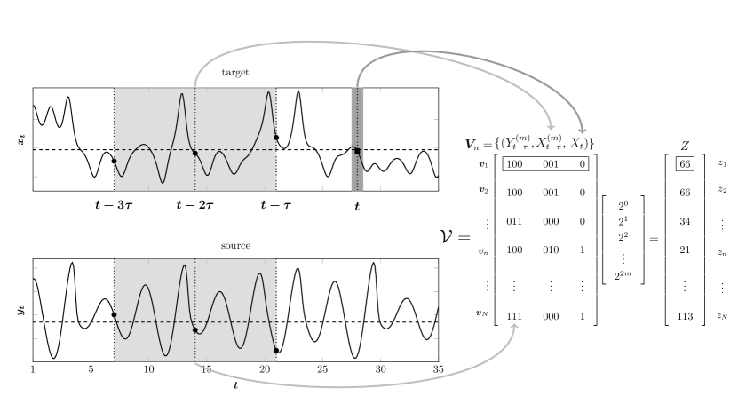
Figure 1: Diagram to obtain the sequence $z_{n}$ to calculate the entropy rate $h\left({Y}_{t-\tau}^{\left(m\right)},{X}_{t-\tau}^{\left(m\right)},X_{t}\right)$. The matrix $\mathcal{V}$ is obtained by embedding ($m=3$) the binarized version of $x_{t}$ and $y_{t}$. The median values of both time series are shown as horizontal dashed lines.

The Transfer Entropy is able to assess the amount of information transferred from process $Y$ (driver/source) to process $X$ (driven/target). It is defined as [5, 6, 15, 1]:

$$\text{{T}}_{Y\to X}^{\left(m\right)}= \phantom{+}H\left({X}_{t-\tau}^{\left(m\right)},{Y}_{t-\tau}^{\left(m\right)}\right)-H\left(X_{t},{X}_{t-\tau}^{\left(m\right)},{Y}_{t-\tau}^{\left(m\right)}\right),$$

$$+H\left(X_{t},{X}_{t-\tau}^{\left(m\right)}\right)-H\left({X}_{t-\tau}^{\left(m\right)}\right).$$ (4)

The parameter $m$ is commonly called the history length or embedding dimension and $\tau$ is the lag or embedding lag [6]. $\text{{T}}_{Y\to X}^{\left(m\right)}$ quantifies the amount of information contained in the $m$-past states of process $Y$ (${Y}_{t-\tau}^{\left(m\right)}$) about the current state of the process $X$ ($X_{t}$), that is not already explained by the $m$-past states of process $X$ (${X}_{t-\tau}^{\left(m\right)}$). This measure is asymmetric ($\text{{T}}_{Y\to X}^{\left(m\right)}\neq\text{{T}}_{X\to Y}^{\left(m\right)}$) and increases along with the coupling level, allowing to determine the direction and strength of the information flow [5].

In [3] Amblard et al. suggest that under stationarity conditions the TE can be considered as an information flow rate. This idea leads to the definition of Transfer Entropy Rate [3, 4, 16]:

$$\text{{t}}_{Y\to X}^{\left(m\right)} \equiv h\left(X\right)-h\left(X|Y\right),$$

$$=h\left(X_{t},{X}_{t-\tau}^{\left(m\right)}\right)-h\left({Y}_{t-\tau}^{\left(m\right)},{X}_{t-\tau}^{\left(m\right)},X_{t}\right),$$ (5)

where $h\left(X\right)$ is the entropy rate of $X$ and $h\left(X|Y\right)$ is the conditional entropy rate [16]:

$$h\left(X|Y\right) \equiv\mathop{\lim}\limits_{m\to\infty}\!{H\left(X_{t}\big{|}{X}_{t-\tau}^{\left(m\right)},{Y}_{t-\tau}^{\left(m\right)}\right)},$$

$$=\mathop{\lim}\limits_{m\to\infty}\!{\frac{H\left({Y}_{t-\tau}^{\left(m\right)},{X}_{t-\tau}^{\left(m\right)},X_{t}\right)}{m}},$$

$$=h\left({Y}_{t-\tau}^{\left(m\right)},{X}_{t-\tau}^{\left(m\right)},X_{t}\right).$$

The TER lies between zero and the entropy rate of the target $X$, being equal to zero if $X$ and $Y$ are independent [16].

If the processes $X$ and $Y$ had no relationship, then $\text{{t}}_{Y\to X}^{\left(m\right)}$ should be equal to zero. However, in practical applications, the estimation of $\text{{t}}_{Y\to X}^{\left(m\right)}$ could present a bias due to the finite length of the data. Some authors [6] proposed to correct this bias by empirically finding the distribution of the surrogate measurement $\text{{\^{t}}}_{\widehat{Y}\to X}^{\left(m\right)}$. The surrogate data must be generated in such a way that the temporal correlation between the source and the target is destroyed but statistical properties and the temporal structure of both processes are preserved [5, 6]. Note that only the second term in equation (5) depends on the source, so the surrogate transfer entropy from $Y$ to $X$ is defined as:

$$\text{{\^{t}}}_{\widehat{Y}\to X}^{\left(m\right)}=-\left<h_{k}\left({\hat{Y}}_{t-\tau}^{\left(m\right)},{X}_{t-\tau}^{\left(m\right)},X_{t}\right)\right>_{K},$$ (6)

where ${\hat{Y}}_{t-\tau}^{\left(m\right)}$ is obtained by redrawing with replacement samples from ${Y}_{t-\tau}^{\left(m\right)}$, and $<\cdot>_{K}$ is the mean value over the $k=1,2,\dots,K$ surrogate realizations.

In order to assess the directionality of the information transport we need to analyze the global TER estimator:

$$\mathcal{T}=\text{{t}}_{Y\to X}^{\left(m\right)}-\text{{t}}_{X\to Y}^{\left(m\right)}-\left(\text{{\^{t}}}_{\widehat{Y}\to X}^{\left(m\right)}-\text{{\^{t}}}_{\widehat{X}\to Y}^{\left(m\right)}\right).$$ (7)

A positive value of $\mathcal{T}$ suggests that the information flow goes from system $Y$ to system $X$, meanwhile a negative value suggests the contrary. Finally, if $\mathcal{T}=0$, there is no information flow between systems.

3 Transfer Entropy Rate Based on Lempel-Ziv Complexity

In this section we formalize our approach to estimate the Transfer Entropy Rate using the Lempel-Ziv complexity. The idea is to estimate the two joint entropy rates on the right-hand side of equation (5) by means of their associated joint Lempel-Ziv complexities. To this end, we propose a methodology based on the construction of delayed embedding vectors from quantized time series. For simplicity in the description of the method we will assume binary time series, although this methodology can be extended to higher quantization levels. Consider two binarized time series ($\alpha=2$) from a coupled system: let $x_{t}=x_{1}\dots x_{T}$ be the target and $y_{t}=y_{1}\dots y_{T}$ be the source. In all the simulations, each time series was binarized with its own median value. Set the parameter $m$ (embedding dimension) and $\tau$ (embedding lag) and create the collection of embedding vectors (see Fig. 1):

$$\bm{V}_{n}=\left\{\left({Y}_{t-\tau}^{\left(m\right)},{X}_{t-\tau}^{\left(m\right)},X_{t}\right)\right\},$$

where:

$$n =1,2,\dots,N,\qquad\text{with}\qquad N=T-m\tau,$$

$$t =m\tau+j,$$

$$\bm{v}_{n} =\left(\bm{y}^{\left(m\right)}_{t-\tau},\bm{x}^{\left(m\right)}_{t-\tau},x_{t}\right),$$

$$\bm{x}^{\left(m\right)}_{t-\tau} =\left[x_{t-m\tau},\dots,x_{t-2\tau},x_{t-\tau}\right],$$

$$\bm{y}^{\left(m\right)}_{t-\tau} =\left[y_{t-m\tau},\dots,y_{t-2\tau},y_{t-\tau}\right].$$

By construction $\bm{V}_{n}$ is a collection of ${\left(2m+1\right)}\text{-uples}$ and we can define the sequence ${z_{n}=\sum_{i=1}^{2m+1}{2^{i-1}v_{n,i}}}$, over an extended alphabet of size $2^{2m+1}$ (see Fig. 1). Then, the joint entropy rate can be calculated as [7]:

$$h\left({Y}_{t-\tau}^{\left(m\right)},{X}_{t-\tau}^{\left(m\right)},X_{t}\right) =h\left(\bm{V}_{n}\right),$$

$$=h\left(Z\right),$$

$$=\mathop{\lim}\limits_{N\to\infty}\!{\frac{\mathcal{C}_{z_{n}}\left[\ln\left(2^{{2m+1}}\right)+\ln{\mathcal{C}_{z_{n}}}\right]}{N}},$$ (8)

where $\mathcal{C}_{z_{n}}$ is the LZC of the sequence $z_{n}$. This procedure can be followed to estimate the first term of equation (5), considering the collection of embedding vectors ${\bm{V}_{n}=\left\{\left({X}_{t-\tau}^{\left(m\right)},X_{t}\right)\right\}}$ and the sequence ${z_{n}=\sum_{i=1}^{m+1}{2^{i-1}v_{n,i}}}$. Moreover, we can use the same methodology to obtain a surrogate measurement $h_{k}\left({\hat{Y}}_{t-\tau}^{\left(m\right)},{X}_{t-\tau}^{\left(m\right)},X_{t}\right)$. In this case, ${\hat{Y}}_{t-\tau}^{\left(m\right)}$ is obtained by shuffling (or redrawing with replacement) ${Y}_{t-\tau}^{\left(m\right)}$ amongst the set of $\left\{{Y}_{t-\tau}^{\left(m\right)},{X}_{t-\tau}^{\left(m\right)},X_{t}\right\}$ tuples.

3.1 Implementation

As we have mentioned before, our methodology is based on the construction of embedding spaces from time series. In this direction, our algorithm has two parameters: the embedding dimension ($m$) and the embedding lag ($\tau$). As well as other embedding based algorithms, we have found that the best results are achieved when a good reconstruction of the state space is guaranteed [17]. In other words, when $m$ is bigger than the minimum embedding dimension of the system and $\tau$ is large enough so that the various coordinates of the embedding vectors contains as much new information as possible, without being entirely independent. In this sense a good choice of embedding dimension is $m=m_{x}+m_{y}+1$, here $m_{x}$ and $m_{y}$ are estimations of the minimum embedding dimension of $X$ and $Y$, respectively. On the other hand, we propose to use an embedding lag value $\tau=\text{max}\left(\tau_{x},\tau_{y}\right)$, where $\tau_{x}$ and $\tau_{y}$ are the lags that minimize the mutual information function between $x_{t}$ and $x_{t-\tau}$, and between $y_{t}$ and $y_{t-\tau}$, respectively.

The Algorithm 1 describes the steps to calculate the global Transfer Entropy Rate ($\mathcal{T}$), between processes $X$ and $Y$. In the first step both time series, $x_{t}=x_{1}\dots x_{T}$ and $y_{t}=y_{1}\dots y_{T}$, must be binarized. This can be done using measures as the mean value, or the median value, among other options. Consider $x_{t}$ as the target/driven series and $y_{t}$ as the source/driver series and follow steps 3-6 to obtain the TER from $Y$ to $X$ ($\text{{t}}_{Y\to X}^{\left(m\right)}$) and step 7 to obtain its surrogate estimation ($\text{{\^{t}}}_{\widehat{Y}\to X}^{\left(m\right)}$). As it was previously described, to estimate each term in equation (5) we need to embed the binarized time series in spaces with different dimensions. Considering the one with the greatest dimension: $\left\{{Y}_{t-\tau}^{\left(m\right)},{X}_{t-\tau}^{\left(m\right)},X_{t}\right\}$, the embedding vectors in this space can be disposed in a matrix ${\mathcal{V}=\left[{Y}_{t-\tau}^{\left(m\right)},{X}_{t-\tau}^{\left(m\right)},X_{t}\right]}$ (see figure 1). The sequence $z_{n}$ can be expressed as the product:

$$z_{n}=\mathcal{V}\left[2^{0},2^{1},\dots,2^{2m}\right]^{T},$$

and, the entropy rate $h\left({Y}_{t-\tau}^{\left(m\right)},{X}_{t-\tau}^{\left(m\right)},X_{t},\right)$ can be computed using equation (8). Regarding the second term in equation (5), given that the space $\left\{{X}_{t-\tau}^{\left(m\right)},X_{t}\right\}$ is a subspace of $\left\{{Y}_{t-\tau}^{\left(m\right)},{X}_{t-\tau}^{\left(m\right)},X_{t}\right\}$, the sequence $z_{n}$ needed to estimate $h\left({X}_{t-\tau}^{\left(m\right)},X_{t}\right)$ can be computed by taking the product of the last $m+1$ columns of $\mathcal{V}$ with $\left[2^{0},2^{1},\dots,2^{m}\right]^{T}$. Finally, use equation (5) to obtain $\text{{t}}_{Y\to X}^{\left(m\right)}$.

In the step 7 we must generate the surrogate data. Choose a number $K$ of surrogate data sets to be generated and build the surrogate data matrices $\mathcal{V}_{k}=\left[{\hat{Y}}_{t-\tau}^{\left(m\right)},{X}_{t-\tau}^{\left(m\right)},X_{t}\right]$ for $k=1,2,\dots,K$. Here, for each $k$, the sample $\left\{{\hat{Y}}_{t-\tau}^{\left(m\right)}\right\}$ is set by redrawing with repetition from the collection $\left\{{Y}_{t-\tau}^{\left(m\right)}\right\}$. Then, the surrogate Transfer Entropy Rate $\text{{\^{t}}}_{\widehat{Y}\to X}^{\left(m\right)}$ is obtained as the mean value of $h_{k}\left({\hat{Y}}_{t-\tau}^{\left(m\right)},{X}_{t-\tau}^{\left(m\right)},X_{t}\right)$ over all surrogate realizations.

To estimate $\text{{t}}_{X\to Y}^{\left(m\right)}$ (transfer entropy from $X$ to $Y$) and its surrogate $\text{{\^{t}}}_{\widehat{X}\to Y}^{\left(m\right)}$ just set $y_{t}$ as the target series, $x_{t}$ as the source and repeat the procedure described in the steps 3-8. Finally, the global TER must be estimated using equation (7).

Algorithm 1 LeZTER Algorithm.
                                                                                                                                    MATLAB code: https://bitbucket.org/jrinckoar/tentropyrate-lzc/src/master/

1:Binarize the temporal series $x_{t}$ and $y_{t}$ using each median value.

2:Set $x_{t}$ as target/driven series and $y_{t}$ as source/driver series.  

3:Given a value of $m$ and $\tau$, set the matrix of embedding vectors:

$$\mathcal{V}=\left[{Y}_{t-\tau}^{\left(m\right)},{X}_{t-\tau}^{\left(m\right)},X_{t}\right],$$

and obtain the sequence $z_{n}$ (see Fig. 1).

4:Calculate the LZC of $z_{n}$ and the entropy rate $h\left({Y}_{t-\tau}^{\left(m\right)},{X}_{t-\tau}^{\left(m\right)},X_{t}\right)$ using equation (8).

5:Calculate the entropy rate $h\left({X}_{t-\tau}^{\left(m\right)},X_{t}\right)$. Obtain the corresponding $z_{n}$ sequence considering the submatrix of $\mathcal{V}$.

6:Calculate the Transfer Entropy Rate $\text{{t}}_{Y\to X}^{\left(m\right)}$ using equation (5).

7:Set a number $K$ of surrogate data sets. For $k=1,2,\dots,K$ form the matrices:

$$\mathcal{V}_{k}=\left[{\hat{Y}}_{t-\tau}^{\left(m\right)},{X}_{t-\tau}^{\left(m\right)},X_{t}\right].$$

Calculate $h_{k}\left({\hat{Y}}_{t-\tau}^{\left(m\right)},{X}_{t-\tau}^{\left(m\right)},X_{t}\right)$ using equation (8) and $\text{{\^{t}}}_{\widehat{Y}\to X}^{\left(m\right)}$ using equation (6).  

8:Set $y_{t}$ as target series, $x_{t}$ as source series and repeat the steps 3-7 to calculate $\text{{t}}_{X\to Y}^{\left(m\right)}$ and $\text{{\^{t}}}_{\widehat{X}\to Y}^{\left(m\right)}$.  

9:Obtain the global estimation of Transfer Entropy Rate $\mathcal{T}$ using equation (7).

4 Results

We have conducted three simulations using different unidirectional coupled systems: the Henon-Henon, the Lorenz-Lorenz and the Lorenz driven by Rössler. The results presented in Figs. 2, 3 and 4 were computed using values of $m$ and $\tau$ that met the conditions mentioned in Subsection 3.1.

The first system was the coupled Henon-Henon [18, 2]:

$$\begin{cases}y_{1}\left[n+1\right]&=1.4-y_{1}^{2}\left[n\right]-by_{2}\left[n\right],\\ y_{2}\left[n+1\right]&=y_{1}\left[n\right],\\ x_{1}\left[n+1\right]&=1.4-\Big{(}\epsilon y_{1}\left[n\right]+\left(1-\epsilon\right)x_{1}\left[n\right]\Big{)}x_{1}\left[n\right]-bx_{2}\left[n\right],\\ x_{2}\left[n+1\right]&=x_{1}\left[n\right],\\ \end{cases}$$

where $b=0.3$. For the simulation, the coupling parameter $\epsilon$ was varied from zero to one in steps of $0.1$. For each $\epsilon$, $200$ realizations were computed using random initial conditions. The Transfer Entropy Rate was calculated with $m=\left\{2,3,4,5,6,7\right\}$ and $\tau=\left\{1,3,5,7,10\right\}$. This procedure was repeated for data lengths $N=\left\{3000,5000,10000\right\}$.

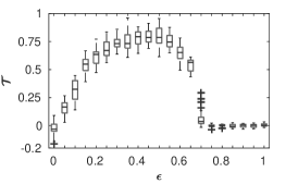
(a)

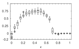
(b)

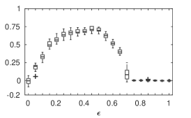
(c)

Figure 2: Henon-Henon coupled system. Boxplot of Transfer Entropy Rate as a function of the coupling parameter $\epsilon$. $\mathcal{T}$ was calculated with $m=5$ and $\tau=1$ for different data lengths: (a) $N=3000$, (b) $N=5000$ and (c) $N=10000$.

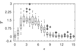
(a)

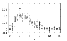
(b)

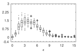
(c)

Figure 3: Lorenz-Lorenz coupled system. Boxplot of Transfer Entropy Rate as a function of the coupling parameter $\epsilon$. $\mathcal{T}$ was calculated with $m=7$ and $\tau=5$ for different data lengths: (a) $N=3000$, (b) $N=5000$ and (c) $N=10000$.

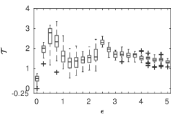
(a)

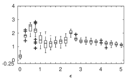
(b)

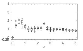
(c)

Figure 4: Rössler-Lorenz coupled system. Boxplot of Transfer Entropy Rate as a function of the coupling parameter $\epsilon$. $\mathcal{T}$ was calculated with $m=7$ and $\tau=10$ for different data lengths: (a) $N=3000$, (b) $N=5000$, and (c) $N=10000$.

The results are shown in the Fig. 2. Each plot presents the global TER ($\mathcal{T}$), calculated with $m=5$ and $\tau=1$, as a function of the coupling parameter $\epsilon$. It can be observed in Fig. 2a ($N=3000$) that the median value of estimator $\mathcal{T}$ is zero for $\epsilon=0$. This is an expected result since there is no information flow between the two systems. Moreover, the median value of $\mathcal{T}$ increases along with the coupling parameter until $\epsilon=0.5$. The positivity of $\mathcal{T}$ points out the correct direction of coupling and its increasing magnitude indicates a rising strength of the coupling. On the other hand, for $\epsilon\geq 0.7$ the median value of $\mathcal{T}$ is zero. For these values of the coupling parameter the Henon-Henon system is synchronized in such a way that both systems are statistically indistinguishable. In this kind of situations, $\mathcal{T}$ is unable to point out any information flow. This behaviour has been already observed on other Transfer Entropy estimators [2, 15, 18]. It can be seen in Figs. 2b and 2c ($N=5000$ and $N=10000$, respectively) that the variance of $\mathcal{T}$ decreases as long as the data length is increased.

For the second simulation we have chosen the Lorenz-Lorenz system:

$$\begin{cases}\dot{y}_{1}&=10\left(-y_{1}+y_{2}\right),\\ \dot{y}_{2}&=\rho_{1}y_{1}-y_{2}-y_{1}y_{3},\\ \dot{y}_{3}&=y_{1}y_{2}-\frac{8}{3}y_{3},\\ \dot{x}_{1}&=10\left(-x_{1}+x_{2}\right)+\epsilon\left(y_{1}-x_{1}\right),\\ \dot{x}_{2}&=\rho_{2}x_{1}-x_{2}-x_{1}x_{3},\\ \dot{x}_{3}&=x_{1}x_{2}-\frac{8}{3}x_{3},\end{cases}$$

where $\rho_{1}=28.5$, $\rho_{2}=27.5$ and $\epsilon\in\left\{0,\dots,15\right\}$. For each value of the coupling parameter, $200$ realization were computed, each one starting from a different initial condition. The numerical integration was performed using the ode45 function of Matlab (algorithm of Dormand and Prince) with step size $\Delta t=0.03$. For each realization the first $10000$ data points where discarded. Then, $\mathcal{T}$ was calculated for all the combination of the parameters: $m=\left\{2,3,4,5,6,7\right\}$ and $\tau=\left\{1,3,5,7,10\right\}$. The above procedure was applied varying the data length $N=\left\{3000,5000,10000\right\}$.

In Fig. 3 is shown estimator $\mathcal{T}$ ($m=7$ and $\tau=5$) as a function of $\epsilon$ for the Lorenz-Lorenz coupled system. For $N=3000$ (Fig. 3a) it can be observed that for uncoupled systems $\epsilon=0$ the median value of $\mathcal{T}\approx 0$. As the coupling parameter increases, $\mathcal{T}$ is positive and grows until the synchronization threshold is reached $\epsilon\approx 12$ [18]. From this point, the value of $\mathcal{T}$ goes toward zero despite the systems are coupled. The same behavior was displayed by the symbolic transfer entropy [19] and other information flow estimators calculated over the same system [18]. As well as in the case of the Henon-Henon coupled system, the variance of $\mathcal{T}$ decreases as the number of data points is increased (figures 3b and 3c).

The third system is the Lorenz driven by Rössler (Rössler-Lorenz) system:

$$\begin{cases}\dot{y}_{1}&=-\alpha\left(y_{2}+y_{3}\right),\\ \dot{y}_{2}&=\alpha\left(y_{1}+0.2y_{2}\right),\\ \dot{y}_{3}&=\alpha\Big{(}0.2+y_{3}\left(y_{1}-5.7\right)\Big{)},\\ \dot{x}_{1}&=10\left(-x_{1}+x_{2}\right),\\ \dot{x}_{2}&=28x_{1}-x_{2}-x_{1}x_{3}+\epsilon y^{\beta}_{2},\\ \dot{x}_{3}&=x_{1}x_{2}-\frac{8}{3}x_{3},\end{cases}$$

where $\alpha=6$, $\beta=2$ and $\epsilon\in\left\{0,0.2,\dots,5\right\}$. For each value of the coupling parameter, $200$ realization using random initial conditions were computed. The numerical integration was performed using the same methodology described for the Lorenz-Lorenz system, but $\Delta t=0.02617$ [15]. The TER was calculated using the same parameter’s values of the afore simulations.

In Fig. 4 the behavior of $\mathcal{T}$ as a function of the coupling parameter for $m=7$ and $\tau=10$ is shown. For this coupled system the synchronization threshold is $\epsilon\approx 2.8$ [18, 20]. It can be observed in Fig. 4a ($N=3000$) that the median value of $\mathcal{T}$ is always positive, even for $\epsilon=0$. This means that the $\mathcal{T}$ estimator is detecting false coupling for $\epsilon=0$. This phenomenon has been also observed in the Symbolic Transfer Entropy [19]. However, the $\mathcal{T}$ estimator is detecting the correct coupling direction. Figs. 4b and 4c display a similar behaviour but notice that the variance of $\mathcal{T}$ decreases.

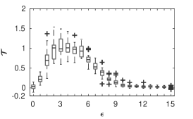
(a)

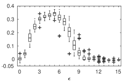
(b)

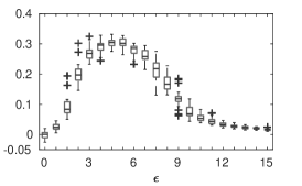
(c)

Figure 5: Comparison of Transfer Entropy Rate estimation with three different methods: (a) Lempel-Ziv’s complexity based method, (b) Symbolic Transfer Entropy and (c) KNN method. Boxplot of the $\mathcal{T}$ as a function of the coupling parameter, calculated for the coupled Lorenz system with $m=5$, $\tau=10$ and $N=10000$.

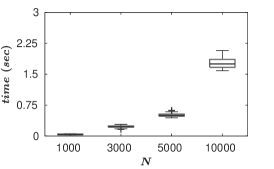
(a)

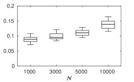
(b)

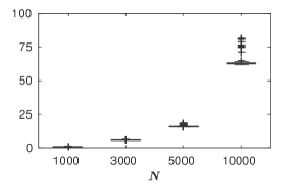
(c)

Figure 6: Computation time for a single as a function of data length ($N$) for different Transfer Entropy Rate estimation methods: (a) Lempel-Ziv’s complexity based method, (b) Symbolic Transfer Entropy and (c) KNN method. The simulation was made using the coupled Lorenz system with $m=5$, $\tau=5$ and $\epsilon=3$.

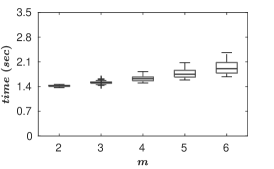
(a)

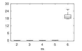
(b)

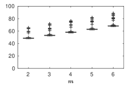
(c)

Figure 7: Computation time as a function of the embedding dimension ($m$) for different Transfer Entropy Rate estimation methods: (a) Lempel-Ziv’s complexity based method, (b) Symbolic Transfer Entropy and (c) KNN method. The simulation was made using the coupled Lorenz system with parameters $N=10000$, $\tau=10$ and $\epsilon=3$.

5 Discussion

There are two methodologies to estimate the Transfer Entropy Rate that are similar to our approach. The first one is the Symbolic Transfer Entropy [19], which finds its foundations in the Permutation Entropy [21]. The second one can be found in [22] and is based on the K-nearest-neighbor (KNN) estimation method proposed by Kraskov et al. [23]. In order to compare our methodology with the ones mentioned above, we have implemented both algorithms and calculated the global TER and the computation time of each one of the $200$ realizations of the coupled Lorenz-Lorenz system. The simulation was done using $m=\left\{2,3,4,5,6\right\}$, $N=\left\{1000,3000,5000,10000\right\}$, $\epsilon=\left\{0,\dots,15\right\}$, $\tau=5$ and $K=30$ surrogate realizations (just for our approach). The simulation was performed in a cluster with 10 nodes, each one has 2 Intel Xeon E5-2670 v3 2.5GHz processors of 12 Cores.

In Fig. 5 we show the global TER as a function of the coupling parameter using the three methods. It can be observed that $\mathcal{T}$ presents a very similar behaviour for all the three methods. However, it is important to notice that for a given $\epsilon$ their values differ. This result strength the hypothesis that our methodology can be used as a information transfer measure.

Results about the comparison of computation times among methodologies can be found in Figs. 6 and 7, where we present a boxplot of the computation time of a single realization as a function of the data lenght and the embedding dimension, respectively. As it can be seen in Figs. 6a, 6b and 6c, the computation time of a single realization, increases exponentially as the data length increases, regardless the employed methodology. Moreover, it can be observed that, for $m=4$, the fastest method is the Symbolic Transfer entropy, followed by our methodology and far away is the KNN approach. On the other hand, Figs. 7a, 7b and 7c show the execution time for a single realization for different embedding dimensions. Notice that the computational cost of each method increases with $m$ in different ways. For our approach the increasing is exponential since the $m$ parameter is linked to the alphabet size in the Lempel-Ziv’s algorithm. We must point out that our methodology outperforms the Symbolic Transfer entropy approach for $m>5$ (compare the computation time in Figs 7a and 7b for $m=6$). This is because the computational cost of the Symbolic Transfer entropy increases with $m$ in a factorial way. This suggests that our methodology has an advantage over the Symbolic Transfer entropy when the analysis of high-dimensional systems is needed. Finally, note for the greatest embedding dimension here studied ($m=8$) and the longest data length ($N=10000$) tested in this simulation, our approach performs a single Transfer Entropy Rate estimation in less than three seconds.

Based on the results, we can conclude that the estimator $\mathcal{T}$ here proposed (equation (7)) is able to detect the direction and strength of the information flow between two coupled ergodic systems. This methodology, based in the LZC, is computationally fast and it does not assume any model for the data. Our results are comparable with those obtained by the Symbolic Transfer Entropy [19] and with the ones reported by Krakovská et al. in [18].

The TER depends on two parameters: $m$ (the history length) and $\tau$ (the lag). For simplicity, we considered that these parameters should be the same for the embedding of both time series, although they can be different [6]. We have observed that the best results are achieved when the values of $m$ and $\tau$ ensure good reconstruction of the state space.

In future studies, we will address the implementation of our methodology using different embedding parameters for $x_{t}$ and $y_{t}$ as well as a different alphabet size.

6 Conclusions

In this article we have presented a new methodology to calculate the Transfer Entropy Rate between two systems based on the Lempel-Ziv’s complexity. Because of the properties of the Lempel-Ziv’s algorithm, we were able to propose a computationally fast methodology to estimate the information flow between two systems. This methodology have been assessed using three unidirectional coupled systems: Henon-Henon system, Lorenz-Lorenz system and Rössler-Lorenz system. The results show that our estimator is able to detect the direction and strength of the information flow.

References

- [1] T. Schreiber, “Measuring information transfer,” Physical Review Letters, vol. 85, no. 2, pp. 461–464, 2000.
- [2] M. Palus, V. Komárek, Z. Hrncír, and K. Sterbová, “Synchronization as adjustment of information rates: detection from bivariate time series.” Phys. Rev. E, vol. 63, 2001.
- [3] P.-O. Amblard and O. J. J. Michel, “Relating Granger causality to directed information theory for networks of stochastic processes,” no. March 2015, 2009.
- [4] P. O. Amblard and O. J. Michel, “On directed information theory and Granger causality graphs,” Journal of Computational Neuroscience, vol. 30, no. 1, pp. 7–16, 2011.
- [5] A. Kaiser and T. Schreiber, “Information transfer in continuous processes,” Physica D: Nonlinear Phenomena, vol. 166, no. 1-2, pp. 43–62, 2002.
- [6] T. Bossomaier, L. Barnett, M. Harré, and J. T. Lizier, An Introduction to Transfer Entropy. Springer International Publishing, 2016.
- [7] S. Zozor, P. Ravier, and O. Buttelli, “On Lempel-Ziv complexity for multidimensional data analysis,” Physica A: Statistical Mechanics and its Applications, vol. 345, no. 1-2, pp. 285–302, 2005.
- [8] J.-L. Blanc, L. Pezard, and A. Lesne, “Delay independence of mutual-information rate of two symbolic sequences,” Phys. Rev. E, vol. 84, no. 3, p. 036214, 2011.
- [9] E. Estevez-Rams, R. Lora Serrano, B. Aragón Fernández, and I. Brito Reyes, “On the non-randomness of maximum Lempel Ziv complexity sequences of finite size,” Chaos, vol. 23, no. 2, 2013.
- [10] H. G. Schuster and W. Just, Deterministic Chaos. Wiley-VCH Verlag GmbH & Co. KGaA, 2005.
- [11] C. Granero-Belinchon, S. G. Roux, P. Abry, M. Doret, and N. B. Garnier, “Information theory to probe intrapartum fetal heart rate dynamics,” Entropy, vol. 19, no. 12, pp. 1–19, 2017.
- [12] A. Papoulis and S.-U. Pillai, Probabilities, Random Variables, and Stochastic Processes. Tata McGraw-Hill Education, 1991.
- [13] T. M. Cover and J. A. Thomas, Elements of information theory. John Wiley & Sons, 2012.
- [14] A. Lempel and J. Ziv, “On the Complexity of Finite Sequences,” IEEE Transactions on Information Theory, vol. 22, no. 1, pp. 75–81, 1976.
- [15] M. Paluš and M. Vejmelka, “Directionality of coupling from bivariate time series: How to avoid false causalities and missed connections,” Phys. Rev. E, vol. 75, no. 5, pp. 1–14, 2007.
- [16] T. Haruna and K. Nakajima, “Symbolic transfer entropy rate is equal to transfer entropy rate for bivariate finite-alphabet stationary ergodic Markov processes,” European Physical Journal B, vol. 86, no. 5, 2013.
- [17] M. Small, Applied Nonlinear Time Series Analysis: Applications in Physics, Physiology and Finance. World Scientific, 2005.
- [18] A. Krakovská, J. Jakubík, H. Budáčová, and M. Holecyová, “Causality studied in reconstructed state space. Examples of uni-directionally connected chaotic systems,” arXiv preprint arXiv:1511.00505, pp. 1–41, 2015.
- [19] M. Staniek and K. Lehnertz, “Symbolic transfer entropy,” Physical Review Letters, vol. 100, no. 15, pp. 1–4, 2008.
- [20] R. Q. Quiroga, J. Arnhold, and P. Grassberger, “Learning driver-response relationships from synchronization patterns,” Phys. Rev. E, vol. 61, no. 5, pp. 5142–5148, 2000.
- [21] C. Bandt and B. Pompe, “Permutation entropy: a natural complexity measure for time series,” Physical Review Letters, vol. 88, no. 17, p. 174102, 2002.
- [22] M. Lindner, V. Priesemann, R. Vicente, and M. Wibral, “TRENTOOL : a Matlab open source toolbox to analyse information flow in time series data with transfer entropy,” BMC Neuroscience, vol. 12, no. 119, 2011.
- [23] A. Kraskov, H. Stögbauer, and P. Grassberger, “Estimating mutual information,” Phys. Rev. E, vol. 69, no. 6, p. 16, 2004.