A tail-regression estimator for heavy-tailed distributions of known tail indices
and its application to continuum quantum Monte Carlo data

Abstract

Standard statistical analysis is unable to provide reliable confidence intervals on expectation values of probability distributions that do not satisfy the conditions of the central limit theorem. We present a regression-based estimator of an arbitrary moment of a probability distribution with power-law heavy tails that exploits knowledge of the exponents of its asymptotic decay to bypass this issue entirely. Our method is applied to synthetic data and to energy and atomic force data from variational and diffusion quantum Monte Carlo calculations, whose distributions have known asymptotic forms [J. R. Trail, Phys. Rev. E 77, 016703 (2008); A. Badinski et al., J. Phys.: Condens. Matter 22 074202 (2010)]. We obtain convergent, accurate confidence intervals on the variance of the local energy of an electron gas and on the Hellmann-Feynman force on an atom in the all-electron carbon dimer. In each of these cases the uncertainty on our estimator is 45% and 60 times smaller, respectively, than the nominal (ill-defined) standard error.

I Introduction

Monte Carlo integration methods Kalos_Whitlock_montecarlo_1986 allow the evaluation of arbitrarily complicated high-dimensional integrals using random, discrete samples of the integrand. Besides the need to correct for serial correlation flyvbjerg_reblock_1989 ; Jonsson_reblock_2018 , the statistical analysis of these random samples is usually straightforward, and the final result of a Monte Carlo calculation is typically computed as a standard mean with an accompanying standard error, defining a confidence interval on the quantity of interest Stroock_probability_1993 . However there are problems for which the integrand diverges in such manner as to render these confidence intervals invalid.

This is the case in continuum quantum Monte Carlo (QMC) methods Ceperley_DMC_1980 ; Foulkes_QMC_2001 , a prominent family of tools for studying correlated many-body systems. Given a trial wave function $\Psi({\bf R})$, the variational Monte Carlo (VMC) method evaluates the expectation value of an observable $\hat{A}$ by accumulating its local value $A({\bf R})$ at random real-space configurations of the particles in the system, $\{\bf R\}$, distributed according to $\left|\Psi({\bf R})\right|^{2}$. The diffusion Monte Carlo (DMC) method samples the lowest-energy wave function $\Phi({\bf R})$ with the same nodal structure as $\Psi({\bf R})$ by stochastic projection according to the imaginary-time Schrödinger equation, and yields more accurate estimates of observables than VMC. The stochastic integration employed by these methods allows using trial wave functions that are not analytically integrable, providing extraordinary flexibility and compactness in the description of many-body correlations LopezRios_Jastrow_2012 ; LopezRios_backflow_2006 ; Bajdich_Pfaffians_2006 . The VMC and DMC methods are routinely used to solve electronic structure and quantum chemistry problems Ceperley_DMC_1980 ; Seth_atoms_2011 ; Drummond_hydrogen_2015 .

The mismatch between the nodes of the trial wave function, $\{{\bf R}:~{}\Psi({\bf R})=0\}$, and those of the true ground-state wave function of the system are the main source of outliers in the local energy distribution sampled in QMC, resulting in heavy tails Panharipande_helium_1986 ; Trail_htail_2008 that preclude the evaluation of meaningful confidence intervals on the estimated variance of the local energy. The local atomic force, comprising a Hellmann-Feynman force Feynman_forces_1939 and a Pulay term Pulay_forces_1969 ; Casalegno_forces_2003 , has heavy tails arising both from the divergence of the electron-nucleus potential energy in all-electron systems Badinski_forces_2010 and from the nodal error, which prevent the evaluation of meaningful confidence intervals on the estimated expectation value of the force.

Various methods have been proposed to circumvent the statistical hurdles in the evaluation of atomic forces in QMC. Modified estimators of the force satisfying a zero-variance principle have been proposed Assaraf_zero-variance_1999 ; Assaraf_forces_2001 ; Assaraf_forces_2003 ; Per_forces_2008 ; Badinski_zero-variance_2008 that substantially reduce the magnitude of the heavy tails in the local force distribution. Force estimation methods based on the use of pseudopotentials Badinski_pp_forces_2007 ; Badinski_pp_forces_2008 can eliminate the problematic behavior of the Hellmann-Feynman force Badinski_forces_2010 , as does the fitting approach proposed by Chiesa et al. Chiesa_force_density_2005 . However, some of these methods involve approximations, and none of them addresses the heavy tails in the local Pulay force distribution, and therefore the total force remains affected by an infinite-variance problem. The reweighted approach proposed by Attaccalite and Sorella Attaccalite_reweight_2008 does prevent the Pulay force from diverging, but it involves modifying the sampling distribution and is therefore not applicable in DMC.

Tail-index estimation methods Hill_TIE_1975 ; Beirlant_TIE_1996 ; Kratz_qq_1996 ; Baek_TIE_2010 allow the exponent governing the asymptotic behavior of heavy-tailed probability distributions to be estimated from statistical samples. This prior work, combined with knowledge of the exact asymptotic form of the tails of the local energy Trail_htail_2008 and local force Badinski_forces_2010 distributions, provides us with the foundation to develop the tail-regression estimator (TRE) for heavy-tailed distributions. We demonstrate the application of this technique to VMC and DMC data, for which we are able to obtain forces and local energy variances not affected by the infinite-variance problem.

The rest of this paper is structured as follows. We review the properties of the heavy tails of the local energy and local force distributions in section II. In section III we discuss the standard method for estimating an expectation value from a statistical sample, and we propose our tail-regression estimator in section IV. The application of our methodology is illustrated in section V using model distributions of known statistical properties. Finally, we present the results of applying our method to the VMC energy of a homogeneous electron gas and the VMC and DMC atomic force on an atom in the all-electron C₂ molecule in sections VI and VII, and our conclusions are stated in section VIII.

II Heavy tails in quantum Monte Carlo

We explore the formal definition of expectation values in QMC to allow the characterization of the resulting heavy-tailed distributions. For simplicity, we restrict our analysis to the VMC method until Section VII, in which we discuss the application of our methodology to DMC data. Note that we ignore serial correlation in this work.

Given a trial wave function $\Psi({\bf R})$, a VMC calculation evaluates the expectation value

$$\langle A\rangle=\frac{\int\Psi^{*}({\bf R})\hat{A}\Psi({\bf R})\,{\rm d}{\bf R}}{\int|\Psi({\bf R})|^{2}\,{\rm d}{\bf R}}\;,$$ (1)

by generating electronic configurations $\{\bf R\}$ according to the distribution

$$P_{\bf R}({\bf R})=\frac{|\Psi({\bf R})|^{2}}{\int|\Psi({\bf R})|^{2}\,{\rm d}{\bf R}}\;,$$ (2)

and evaluating the local values $A({\bf R})=\Psi^{-1}({\bf R})\hat{A}\Psi({\bf R})$ of observable $\hat{A}$. The VMC expectation value can be recast as

$$\langle A\rangle=\int_{-\infty}^{\infty}P_{A}(A)A\,{\rm d}A\;,$$ (3)

where

$$P_{A}(A)=\int_{\partial\Omega(A)}\frac{P_{\bf R}({\bf R})}{|\nabla_{\bf R}A({\bf R})|}\,{\rm d}^{dN-1}{\bf R}\;,$$ (4)

where $d$ is the dimensionality of the system, $N$ is the number of electrons, and $\partial\Omega(A)$ is the $(dN-1)$-dimensional region of configuration space where $A({\bf R})=A$.

The local value of some important observables diverge at certain configurations, and it is often possible to characterize the asymptotic behavior of $P_{A}(A)$ from knowledge of the analytical form of $\Psi({\bf R})$ near to these configurations. We summarize the relevant properties of the local energy and the local atomic force below.

II.1 Local energy

Consider the Hamiltonian of a molecular system in Hartree atomic units ($\hbar=m_{\rm e}=|e|=4\pi\epsilon_{0}=1$),

$$\hat{H}({\bf R})=-\frac{1}{2}\sum_{i}\nabla_{i}^{2}+\sum_{i,j>i}\frac{1}{r_{ij}}+\sum_{i,I}\frac{-Z_{I}}{r_{iI}}+\sum_{I,J>I}\frac{Z_{I}Z_{J}}{r_{IJ}}\;,$$ (5)

where $r_{ij}$ is the distance between the $i$th and $j$th electrons, $r_{iI}$ is the distance between the $i$th electron and the $I$th nucleus, $r_{IJ}$ is the distance between the $I$th and $J$th nuclei, and $Z_{I}$ is the atomic number of the $I$th nucleus.

The situations in which the local energy $E({\bf R})=\Psi^{-1}({\bf R})\hat{H}({\bf R})\Psi({\bf R})$ diverges were classified in detail by Trail Trail_htail_2008 . The divergence of the Coulomb potential at electron-nucleus and electron-electron coalescence points, $r_{iI}\to 0$ and $r_{ij}\to 0$ respectively, can be neutralized by constraining the trial wave functions to obey the Kato cusp conditions Kato_cusp_1957 under which the kinetic energy exactly cancels the potential energy at two-body coalescence points. The remaining divergences of the local energy arise when $\Psi({\bf R})\to 0$ but $\Psi$ is not locally identical to an eigenstate of $\hat{H}$, since $\hat{H}({\bf R})\Psi({\bf R})$ can be finite where $\Psi({\bf R})$ is zero.

Mismatches between the nodes of $\Psi({\bf R})$ and $\hat{H}({\bf R})\Psi({\bf R})$ are responsible for the asymptotic behavior Trail_htail_2008

$$P_{E}(E)=c_{0}|E-E_{0}|^{-4}+c_{1}|E-E_{0}|^{-5}+\ldots\;,$$ (6)

when $|E|\to\infty$, where $E_{0}$ is the exact ground state energy and $\{c_{i}\}$ are unknown coefficients. The coefficients of even powers of $|E-E_{0}|$ in the left ($E\to-\infty$) and right ($E\to+\infty$) tails of $P_{E}(E)$ have equal coefficients, $c_{2n}^{\rm L}=c_{2n}^{\rm R}$, while those of odd powers are of the same magnitude but of opposite signs, $c_{2n+1}^{\rm L}=-c_{2n+1}^{\rm R}$.

The expectation value of the energy itself can be evaluated with standard estimators without problems, but these yield unreliable confidence intervals on the variance of the local energy. The variance of the local energy is an important quantity since it is directly related to the quality of the trial wave function, and is routinely used in wave function optimization Umrigar_varmin_1988 , as well as in the “variance extrapolation” technique that attempts to estimate the zero-variance (exact wave function) limit of expectation values Holzmann_ueg_2003 . We discuss the specific issues with the variance of the local energy in section III.

II.2 Local force

The force exerted by the electrons and the other nuclei on the $I$th nucleus of a system along the $x$ direction is $\langle\hat{F}_{x,I}\rangle=-{\rm d}\langle\hat{H}\rangle/{\rm d}x_{I}$, where $x_{I}$ is the $x$ Cartesian coordinate of the $I$th nucleus. Dropping the $I$ and $x$ labels, the local force can be expressed as

$$F({\bf R})=F_{\rm HFT}({\bf R})+F_{\rm P}({\bf R})\;,$$ (7)

where the Hellmann-Feynman force is

$$\begin{split}F_{\rm HFT}({\bf R})&=-\Psi^{-1}({\bf R})\frac{\partial\hat{H}({\bf R})}{\partial x}\Psi({\bf R})\\ &=\sum_{i}\frac{-Z_{I}x_{iI}}{r_{iI}^{3}}+\sum_{J\neq I}\frac{Z_{I}Z_{J}x_{IJ}}{r_{IJ}^{3}}\;,\end{split}$$ (8)

and the Pulay force is

$$F_{\rm P}({\bf R})=-2\Psi^{-1}({\bf R})\left[E({\bf R})-\langle\hat{H}\rangle\right]\frac{\partial\Psi({\bf R})}{\partial x}\;.$$ (9)

Optionally, a variance-reduction term which satisfies a zero-variance principle Assaraf_forces_2003 ,

$$F_{\rm ZV}({\bf R})=-\Psi^{-1}({\bf R})\left[{\hat{H}}({\bf R})-E({\bf R})\right]\frac{\partial\Psi({\bf R})}{\partial x}\;,$$ (10)

can be added to Eq. 7. This term does not alter the expectation value of the force but reduces the extent of the fluctuations of the local Hellmann-Feynman force.

The local Hellmann-Feynman force diverges at electron-nucleus coalescence points, and its distribution exhibits a power-law tail of the form

$$P_{F_{\rm HFT}}(F)=c_{0}|F-F_{0}|^{-5/2}+c_{1}|F-F_{0}|^{-3}+\ldots\;,$$ (11)

when $|F|\to\infty$, where $F_{0}$ is a constant and $\{c_{i}\}$ are unknown coefficients. The coefficients of the leading-order term on the left and right tails are equal, $c_{0}^{\rm L}=c_{0}^{\rm R}$, and the rest are asymmetric.

If the wave function satisfies the electron-nucleus Kato cusp conditions Ma_cusp_2005 the zero-variance term exactly cancels this divergence Per_forces_2008 , but, like for the local energy, the mismatch between the nodes of $\Psi(\bf R)$ and $\hat{H}({\bf R})\Psi({\bf R})$ is responsible for the heavy tails in the distribution of the local values of the Pulay and zero-variance terms, and hence of the total force, which satisfies Badinski_forces_2010

$$P_{F}(F)=c_{0}|F-F_{0}|^{-5/2}+c_{1}|F-F_{0}|^{-3}+\ldots\;,$$ (12)

when $|F|\to\infty$, where $F_{0}$ is a constant and $\{c_{i}\}$ are unknown coefficients exhibiting no symmetry.

A somewhat different scenario arises if nondivergent pseudopotentials are used in place of the electron-nucleus Coulomb potential Trail_pp1_2015 ; Trail_pp2_2017 and the local force estimation is consequently adjusted Badinski_pp_forces_2007 ; Badinski_pp_forces_2008 . In this case the local Hellmann-Feynman force exhibits less problematic heavy tails of leading order $|F-F_{0}|^{-4}$ Badinski_forces_2010 , but since the Pulay term is unaffected by the use of pseudopotentials the local total force remains of the form of Eq. 12.

III Standard estimation of an expectation value

The expectation value of an observable whose local value $A$ is distributed according to $P_{A}(A)$ is

$$\langle A\rangle=\int_{-\infty}^{\infty}P_{A}(A)A\,{\rm d}A\;,$$ (13)

and the variance of $A$ is the expectation value of $\left(A-\langle A\rangle\right)^{2}$,

$${\rm Var}[A]=\sigma^{2}=\int_{-\infty}^{\infty}P_{A}(A)\left(A-\langle A\rangle\right)^{2}\,{\rm d}A\;.$$ (14)

The integrals in Eqs. 13 and 14 must be nondivergent for the expectation value and variance of $A$ to be well-defined. Therefore, probability distributions with asymptotic behavior $P_{A}(A)\sim|A|^{-\mu}$ as $|A|\to\infty$ have no well-defined expectation value or variance for $\mu\leq 2$, and have a well-defined expectation value but no well-defined variance for $2<\mu\leq 3$. Note that a function with $\mu\leq 1$ is not a valid probability distribution as it cannot be normalized.

Let $\{A_{m}\}_{m=1}^{M}$ be a sample of $M$ independent random variables identically distributed according to $P_{A}(A)$. The standard estimator for Eq. 13 is the sample mean,

$$\bar{A}=\frac{1}{M}\sum_{m=1}^{M}A_{m}\;,$$ (15)

and the standard estimator for Eq. 14 is the sample variance,

$$S^{2}=\frac{\sum_{m=1}^{M}(A_{m}-{\bar{A}})^{2}}{M-1}\;.$$ (16)

The uncertainty on $\bar{A}$ is the standard error $\sigma_{\bar{A}}=S/\sqrt{M}$. This poses a problem for distributions of leading-order exponent $2<\mu\leq 3$: despite having a well-defined expectation value according to Eq. 13, its standard estimator has a divergent uncertainty because it is defined in terms of the divergent variance of Eq. 14.

In this regime $P_{A}(A)$ does not satisfy the conditions of the central limit theorem that would guarantee the asymptotic normality of confidence intervals built from the standard mean and standard error Stroock_probability_1993 . Instead, $P_{A}(A)$ satisfies the law of large numbers, which states that the standard mean does converge to the expectation value at infinite sample size but confidence intervals cannot be constructed using the standard error as finite sample sizes.

A similar issue affects the estimator of the variance itself. Even though the variance is well-defined for $\mu>3$, the variance on the estimator of the variance is

$${\rm Var}[S^{2}]=\frac{1}{M}\left(m_{4}-\frac{M-3}{M-1}\sigma^{4}\right)\;,$$ (17)

where $m_{4}$ is the fourth-order central moment of $P_{A}(A)$, which diverges for distributions of leading-order exponent $\mu\leq 5$, leading to a divergent uncertainty on the $S^{2}$ estimator of the variance.

IV Tail-regression estimator

As outlined in the previous section, the uncertainty on the standard estimator of a moment of a probability distribution involves the estimator of a higher-order moment, which might be divergent even though the moment of interest is well-defined. We therefore propose an alternative estimator of the moment of a heavy-tailed probability distribution that exploits knowledge of its analytical asymptotic form to yield well-defined confidence intervals whenever the moment itself is well defined.

Without loss of generality we focus on distributions with a right heavy tail; the extension of our analysis to distributions with left and both left and right heavy tails is straightforward. In particular, we consider a probability distribution exhibiting a right tail of asymptotic form

$$P_{A}(A)=\sum_{n}c_{n}\left|A-A_{0}\right|^{-\mu-n\Delta}\;,$$ (18)

when $A\to\infty$, where the leading-order exponent $\mu$ and exponent increment $\Delta>0$ are assumed to be known analytically, as is the case for local energies, with $\mu=4$ and $\Delta=1$ Trail_htail_2008 , and for local forces, with $\mu=5/2$ and $\Delta=1/2$ Badinski_thesis_2008 . The specific value of $\Delta$ is not critical for the correct description of the asymptote by Eq. 18, and can be assumed to be unity, but the accuracy of a truncated expansion strongly depends on $\Delta$. In other words, the bias incurred by choosing a suboptimal value of $\Delta$ can be made arbitrarily small by using a larger expansion. In Eq. 18 $\{c_{n}\}$ are unknown coefficients, and $A_{0}$ is an unknown parameter which is assumed to lie close to the “center” of the distribution.

IV.1 Validity of asymptote with approximate $A_{0}$

First, we address the fact that $A_{0}$ is an unknown nonlinear parameter in Eq. 18 and will have to be approximated. Let $A_{\rm c}$ be an approximation to $A_{0}$ such that $A_{0}=A_{\rm c}+\varepsilon$, where $\varepsilon$ is a small error. Assuming for simplicity that $\Delta^{-1}$ is an integer and expanding to first order in $\varepsilon$ we find

$$\begin{split}P_{A}(A)=&\sum_{n}c_{n}|A-A_{\rm c}-\varepsilon|^{-\mu-n\Delta}\\ \approx&\sum_{n}c_{n}|A-A_{\rm c}|^{-\mu-n\Delta}\\ &+\varepsilon\sum_{n}c_{n}(\mu+n\Delta)|A-A_{\rm c}|^{-\mu-n\Delta-1}\\ =&\sum_{n}c_{n}^{\prime}|A-A_{\rm c}|^{-\mu-n\Delta}=P_{A}^{\prime}(A)\;,\\ \end{split}$$ (19)

where

$$c_{n}^{\prime}=\left\{\begin{array}[]{l@{\,,\quad}l}c_{n}&n<\Delta^{-1}\\ c_{n}+\varepsilon c_{n-\Delta^{-1}}(\mu+n\Delta-1)&n\geq\Delta^{-1}\\ \end{array}\right.\;.$$ (20)

The asymptotic expression $P_{A}^{\prime}(A)$ has the same form as $P_{A}(A)$, albeit with modified coefficients $c_{n}^{\prime}$ for $n\geq\Delta^{-1}$. We shall therefore proceed with the derivation of our estimator using $P_{A}^{\prime}(A)$ as the asymptote, dropping the primes from the notation for clarity. This effectively amounts to replacing $A_{0}$ with $A_{\rm c}$, which in practice we set to the sample median.

IV.2 Estimator

In order to develop our estimator, we start by assuming that there exists a threshold $A_{\rm R}$ such that for $A>A_{\rm R}$ the probability distribution is accurately represented by an expansion of order $n_{\rm R}$,

$$P_{A}(A)=\sum_{n=0}^{n_{\rm R}}c_{n}\left|A-A_{\rm c}\right|^{-\mu-n\Delta}\,,\quad A>A_{\rm R}\;.$$ (21)

The integral of Eq. 13 can be partitioned at $A_{\rm R}$ into central and right-tail contributions,

$$\langle A\rangle=\int_{-\infty}^{A_{\rm R}}P_{A}(A)A\,{\rm d}A+\int_{A_{\rm R}}^{\infty}P_{A}(A)A\,{\rm d}A\;.$$ (22)

Let $\{A_{m}\}$ be a sample of $M$ independent random variables identically distributed according to $P_{A}(A)$, $\{A^{(m)}\}$ the corresponding order statistics, i.e., the re-indexed version of $\{A_{m}\}$ such that $A^{(1)}>A^{(2)}>\ldots>A^{(M)}$, $M_{\rm C}$ the number of data in the central region $A<A_{\rm R}$, and $M_{\rm R}=M-M_{\rm C}$ the number of data in the tail. We define the tail-regression estimator of $\langle A\rangle$ as

$${\cal A}=\frac{1}{M}\sum_{m>M_{\rm R}}A^{(m)}+\sum_{n=0}^{n_{\rm R}}c_{n}\int_{A_{\rm R}}^{\infty}\left|A-A_{\rm c}\right|^{-\mu-n\Delta}A\,{\rm d}A\;.$$ (23)

The integrals in Eq. 23 are nondivergent for $\mu>2$ and can be evaluated analytically,

$$\begin{gathered}\int_{A_{\rm R}}^{\infty}|A-A_{\rm c}|^{-\mu-n\Delta}A\,{\rm d}A=\\ =\left[\frac{|A_{\rm R}-A_{\rm c}|^{-\mu-n\Delta+2}}{\mu+n\Delta-2}+A_{\rm c}\frac{|A_{\rm R}-A_{\rm c}|^{-\mu-n\Delta+1}}{\mu+n\Delta-1}\right]\;.\end{gathered}$$ (24)

The parameters $\{c_{n}\}$ in Eq. 23 can be obtained by regression of $\{A^{(m)}\}_{m=1}^{M_{\rm R}}$ to Eq. 21. Since $\cal A$ is linear in $\{c_{n}\}$, the distribution of $\cal A$ follows that of $\{c_{n}\}$. This implies that if the regression coefficients are asymptotically normally distributed, ${\cal A}$ will also be asymptotically normally distributed. We will address the distribution of regression coefficients in section IV.4. We regard $A_{\rm R}$, and $n_{\rm R}$ as external parameters that we deal with separately, see section IV.5, and do not contribute to the uncertainty on ${\cal A}$.

Analogously, we define the tail-regression estimators of the norm,

$${\cal W}=\frac{M_{\rm C}}{M}+\sum_{n=0}^{n_{\rm R}}c_{n}\int_{A_{\rm R}}^{\infty}\left|A-A_{\rm c}\right|^{-\mu-n\Delta}\,{\rm d}A\;,$$ (25)

and of the variance of the distribution,

$$\begin{split}{\cal V}&=\frac{1}{M-1}\sum_{m>M_{\rm R}}(A^{(m)}-{\cal A})^{2}\\ &+\sum_{n=0}^{n_{\rm R}}c_{n}\int_{A_{\rm R}}^{\infty}\left|A-A_{\rm c}\right|^{-\mu-n\Delta}(A-{\cal A})^{2}\,{\rm d}A\;.\end{split}$$ (26)

These integrals can likewise be evaluated analytically. Finally, we note that the threshold $A_{\rm R}$ must lie on the midpoint between two adjacent sample points, $\frac{1}{2}\left(A^{(M_{\rm R})}+A^{(M_{\rm R}+1)}\right)$, to ensure that the central contributions have the correct weight in Eqs. 23, 25, and 26.

We use the bootstrap method Efron_bootstrap_1986 to compute the uncertainty on ${\cal A}$. We generate $n_{\rm bs}$ resamples of $\{A_{m}\}$ with replacement, that is, the $i$th resample $\{A_{m}^{[i]}\}$ contains $M$ elements from $\{A_{m}\}$ drawn at random and uniformly, allowing repetitions. For each resample we evaluate ${\cal A}^{[i]}$, and we evaluate the uncertainty on ${\cal A}$ as the standard deviation of the values of $\{{\cal A}^{[i]}\}$. Estimates of other statistical parameters arising from analysis of $\{A_{m}\}$, including $\cal W$ and $\cal V$, are also obtained in this process. In our applications of the tail-regression estimator we use $n_{\rm bs}=4096$ bootstrap resamples, which provide a $1.1\%$ uncertainty on the estimated uncertainties assuming normality. The computational cost of this approach is proportional to $M\times n_{\rm bs}$.

IV.3 Tail form in $yx$ scale

The framework for our tail-regression procedure is inspired by regression-based tail-index estimation methods Hill_TIE_1975 ; Beirlant_TIE_1996 , discussed in Appendix A. First, note that the complementary cumulative distribution function $\bar{F}_{A}(A)$ associated with $P_{A}(A)$ should be approximately equal to the sample quantiles $q_{m}$,

$$\bar{F}_{A}(A)=\int_{A^{(m)}}^{\infty}P_{A}(A)dA\approx q_{m}\;,$$ (27)

for which we use the symmetric form $q_{m}=\frac{m-1/2}{M}$. Substituting Eq. 21 into Eq. 27 yields

$$\sum_{n=0}^{n_{\rm R}}\frac{c_{n}}{\mu+n\Delta-1}\left|A^{(m)}-A_{\rm c}\right|^{-\mu-n\Delta+1}=q_{m}\;,$$ (28)

which we rearrange as

$$q_{m}\left|A^{(m)}-A_{\rm c}\right|^{\mu-1}=\sum_{n=0}^{n_{\rm R}}\frac{c_{n}}{\mu+n\Delta-1}\left|A^{(m)}-A_{\rm c}\right|^{-n\Delta}\;.$$ (29)

We define

$$\begin{split}y_{m}&=q_{m}\left|A^{(m)}-A_{\rm c}\right|^{\mu-1}\;,\\ x_{m}&=|A^{(m)}-A_{\rm c}|^{-\Delta}\;,\end{split}$$ (30)

which we refer to as “$yx$ scale”, under which Eq. 29 reads

$$y_{m}=\sum_{n=0}^{n_{\rm R}}\frac{c_{n}}{\mu+n\Delta-1}x_{m}^{n}\;,$$ (31)

that is, $y$ is simply a polynomial in $x$. By construction, $y$ must be positive and tend to a finite value as $x\to 0$, $y(0)=c_{0}/(\mu-1)$, and the $n$th derivative of $y(x)$ at $x=0$ is likewise proportional to $c_{n}$.

It is useful to inspect the basic properties of the $yx$ scale we have introduced. For illustration purposes, let

$$H_{\mu}(A)=\frac{\mu\sin\frac{\pi}{\mu}}{2\pi}\frac{1}{1+\left|A\right|^{\mu}}\;,$$ (32)

which for $\mu>2$ is a normalized probability distribution whose expectation value is zero and has the asymptote $|A|^{-\mu}$ as $|A|\to\infty$. In Fig. 1 we show a $yx$-scale plot of the left tail of $M$ independent random numbers identically distributed according to $H_{4}(A)$ at different sample sizes $M$, assuming $\Delta=1$. The exact value $y(0)=0.1501$ is shown as a short-dashed line in each panel.

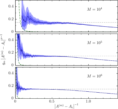
Figure 1: $yx$-scale plot of the left tail of $M$ independent random numbers identically distributed according to $H_{4}(A)$ for sample sizes $M=10^{4}$ (top), $10^{5}$ (middle), and $10^{6}$ (bottom). Shaded areas around curves correspond to the $68.3\%$ and $95.4\%$ confidence intervals obtained from the bootstrap. The short-dashed lines indicate the analytical value of $y(0)$, and the long-dashed lines are the first-quantile lines, $y=\frac{1/2}{M}x^{-3}$, marking the region where the largest value of $A$ falls at each sample size.

The first quantile $q_{1}=1/(2M)$, corresponding to the largest value of $A$ in the sample, gets smaller as $M$ increases, and, as follows from Eq. 30, the extreme point $(x_{1},y_{1})$ satisfies $y_{1}=q_{1}x_{1}^{(1-\mu)/\Delta}$. This curve determines how far left the plot extends, as shown by the long-dashed line in each of the panels of Fig. 1. With increasing $M$ the plot is populated from right to left, gradually producing a better resolved curve near $x=0$.

In Fig. 2 we show $yx$ plots of the $M=10^{6}$ sample used in Fig. 1 in which the $yx$ scale is defined using the exponents $\mu^{\prime}=3$, $4$, and $5$.

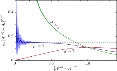
Figure 2: $yx$-scale plot of the left tail of $10^{6}$ independent random numbers identically distributed according to $H_{4}(A)$ using the correct leading-order tail exponent $\mu^{\prime}=\mu=4$ and incorrect values $\mu^{\prime}=3$ and $5$, which respectively go to zero and diverge as $x\to 0$. Shaded areas around curves correspond to the $68.3\%$ and $95.4\%$ confidence intervals obtained from the bootstrap. The short-dashed line indicates the analytical value of $y(0)$.

If the true exponent is underestimated, $\mu^{\prime}<\mu$, the curve goes to zero as $x\to 0$, while overestimating the exponent, $\mu^{\prime}>\mu$, yields a diverging curve at $x\to 0$. Attempting to use $yx$-scale plots to estimate $\mu$ is rudimentary at best, since each possible value must be tested explicitly, and care must be taken in interpreting the large statistical fluctuations of $y$ at small $x$. Tail-index estimation methods Beirlant_TIE_1996 ; Kratz_qq_1996 offer a robust alternative; the regression method of Ref. Beirlant_TIE_1996 produces a reasonable value of $\mu=3.94(2)$ from the data plotted in Fig. 2. Note that the tail-regression estimator relies on analytical knowledge of $\mu$ rather than on its estimation from the sample.

IV.4 Tail regression and weights

We now focus on the regression procedure to ensure a reliable estimation of the fit parameters. It is apparent from Fig. 1 that the distribution of $y$ values at small $x$ about the exact $y(0)$ is skewed towards large $y$, so adequate least-squares weights are needed to ensure the faithfulness of the resulting fit.

Let $r_{m}=w_{m}[y_{m}-y(x_{m})]$ be the least-square residuals, where $w_{m}$ is the least-squares weight applied to the $m$th point, and $\chi^{2}=\frac{1}{M-n_{\rm R}-1}\sum_{m=1}^{M}r_{m}^{2}$ be the least-squares function. Minimizing $\chi^{2}$ with respect to the fit parameters $\{c_{n}\}$ yields the linear system of equations $T{\bf c}={\bf b}$, where

$$\begin{split}(T)_{pq}&=\frac{1}{M}\sum_{m=1}^{M}w_{m}x_{m}^{p+q}\;,\\ ({\bf b})_{p}&=\frac{1}{M}\sum_{m=1}^{M}w_{m}y_{m}x_{m}^{p}\;,\\ ({\bf c})_{p}&=c_{p}\;,\\ \end{split}$$ (33)

and indices $p$ and $q$ run between $0$ and $n_{\rm R}$. The parameter vector is thus

$${\bf c}=T^{-1}{\bf b}=\frac{1}{\det(T)}{\rm adj}(T){\bf b}\;,$$ (34)

where ${\rm adj}(T)$ is the adjugate matrix of $T$ (i.e., the transpose of its cofactor matrix) and $\det(T)$ is its determinant.

The parameters $({\bf c})_{p}$ will be asymptotically normally distributed if $(T)_{pq}$, $({\bf b})_{p}$, and $\det(T)$ are themselves asymptotically normally distributed and $\det(T)$ is nonzero, since Eq. 34 involves sums and multiplications, which preserve asymptotic normality, and a division, which also preserves asymptotic normality if the denominator is strictly nonzero.

We consider weights of the form

$$w_{m}=|A^{(m)}-A_{\rm c}|^{-\gamma(\mu-1)}\;,$$ (35)

where $\gamma$ is a positive constant. Since $x_{m}$ is a negative power of $|A^{(m)}-A_{\rm c}|$, all elements of $T$ and $\det(T)$ are asymptotically normally distributed, but the elements of $\bf b$ need not be. We focus on the $m=1$ contribution to $({\bf b})_{0}$, which is the least likely to exhibit asymptotic normality,

$$w_{1}y_{1}=q_{1}\left|A^{(1)}-A_{\rm c}\right|^{(\mu-1)(1-\gamma)}\;.$$ (36)

Noting that $w_{1}=q_{1}^{\gamma}y_{1}^{-\gamma}$ and that the exact asymptotic value of $y_{1}$ as $M\to\infty$ is by construction $y(0)=c_{0}/(\mu-1)$, the asymptotic limit of $w_{1}y_{1}$ is

$$\xi=q_{1}^{\gamma}\left[\frac{c_{0}}{\mu-1}\right]^{1-\gamma}\;,$$ (37)

where $q_{1}=1/(2M)$ encodes the sample-size dependence.

We now investigate the distribution of values of $w_{1}y_{1}$ about $\xi$. The probability that $|A^{(1)}-A_{\rm c}|$ is bounded from above by $\alpha$ is the probability that the $M$ points in the sample are bounded from above by $A_{\rm c}+\alpha$, that is,

$$\begin{split}{\rm Prob}(|A^{(1)}-A_{\rm c}|\leq\alpha)=&1-\bar{F}_{|A^{(1)}-A_{\rm c}|}(\alpha)\\ =&\left[1-\bar{F}_{A}(A_{\rm c}+\alpha)\right]^{M}\\ \approx&\left(1-c_{0}\alpha^{-\mu+1}\right)^{M}\;,\end{split}$$ (38)

to leading order for large $\alpha$. Differentiating with respect to $\alpha$ yields the probability distribution of the extreme value,

$$P_{|A^{(1)}-A_{\rm c}|}(\alpha)=Mc_{0}(\mu-1)\alpha^{-\mu}\left(1-c_{0}\alpha^{-\mu+1}\right)^{M-1}\;,$$ (39)

and by a change of variable,

$$P_{w_{1}y_{1}/\xi}(\beta)=\frac{\mu-1}{2(1-\gamma)}\beta^{-\frac{2-\gamma}{1-\gamma}}\left[1-\frac{\mu-1}{2M}\beta^{-\frac{1}{1-\gamma}}\right]^{M-1}\;,$$ (40)

assuming $\gamma\neq 1$. At large $\beta$,

$$P_{w_{1}y_{1}/\xi}(\beta)\sim\beta^{-\frac{2-\gamma}{1-\gamma}}\;,$$ (41)

which is a power-law tail for $\gamma<1$, yielding an undefined expectation value for $\gamma\leq 1/2$. Unweighted fits ($\gamma=0$) are therefore numerically ill-conditioned since the residuals are themselves heavy tailed $\sim\beta^{-2}$ regardless of the value of $\mu$. Fit weights with $\gamma>1/2$ must therefore be used.

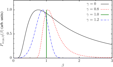
Figure 3: Probability distribution of the values of $w_{1}y_{1}/\xi$, Eq. 40, for various values of $\gamma$, using $\mu=4$ and $M=10^{6}$.

In Fig. 3 we plot $P_{w_{1}y_{1}/\xi}(\beta)$ for various values of $\gamma$. Note that the curve for $\gamma=0$ describes the distribution of values of $y$ in Fig. 1 relative to the analytical value of $y(0)$ along the constant-$q$ lines. The plots for $\gamma=0.8$ and $1.2$ reveal that, while not ill-conditioned, the significant skewness of the distributions makes the first moment of $P_{w_{1}y_{1}/\xi}(\beta)$ differ significantly from the asymptotic expectation value of $1$ in these cases. For $\gamma=1$, $w_{1}y_{1}=q_{1}^{\gamma}$ is $y_{1}$-independent, and the distribution is therefore a delta function peaked at the asymptotic expectation value, as shown in Fig. 3. We therefore use $\gamma=1$ for our fit weights.

We empirically find it advantageous to include a $q_{m}$-dependent factor in the fit weights so as to ensure the continuity of the fit to the probability distribution near $A_{\rm R}$. We choose this factor to be the weights corresponding to the formulation of the Hill estimator of the first-order tail index Hill_TIE_1975 as a regression estimator Beirlant_TIE_1996 , see Eq. 50 in Appendix A. Therefore, our full fit weights are

$$w_{m}=\left(\log\frac{q_{M_{\rm R}+1}}{q_{m}}\right)^{-1}|A^{(m)}-A_{\rm c}|^{-\mu+1}\;.$$ (42)

IV.5 Selecting $n_{\rm R}$ and $A_{\rm R}$

The tail-regression estimator depends parametrically on the expansion order $n_{\rm R}$ and threshold $A_{\rm R}$. In our tests we try several thresholds and converge the fit with respect to the expansion order at each of them. We then choose the value of $A_{\rm R}$ which minimizes the uncertainty on either $\cal V$, if well-defined, or on $\cal A$.

We choose the expansion order heuristically by finding plateaus in $\cal W$, $\cal A$, $\cal V$, and $\chi^{2}$ as a function of $n_{\rm R}$, and selecting the smallest expansion order at which these four functions have converged. To ensure correctness, we further require that ${\cal W}\approx 1$ and $y(x)>0$ within the fit range, and we restrict $n_{\rm R}\geq 1/\Delta$ in order to “absorb” the error incurred by approximating $A_{0}$ by $A_{\rm c}$, as explained in Section IV.1.

Note that we do not set $A_{\rm R}$ directly, but instead set $q_{\rm R}=(M_{\rm R}-1/2)/M$, as keeping the number of sample points in each partition fixed across bootstrap resamples eliminates the variation of the central contribution to $\cal W$, which is statistically advantageous. We choose our values of $q_{\rm R}$ using a grid of equally-spaced values of $-\log q_{\rm R}$. We pick $n_{\rm R}$ and $A_{\rm R}$ using $n_{\rm bs}=256$, and evaluate the final result separately with $n_{\rm bs}=4096$ to avoid selection bias. We illustrate the procedure for choosing $n_{\rm R}$ and $A_{\rm R}$ in section V.1.

IV.6 Two-tailed distributions, symmetry, and constraints

The tail-regression estimator described so far can be modified trivially for distributions with left and right heavy tails. For simplicity we use the same expansion orders and thresholds on both tails, $n_{\rm R}=n_{\rm L}$ and $M_{\rm R}=M_{\rm L}$.

In some important cases, including the local energy and local atomic force in VMC Trail_htail_2008 ; Badinski_forces_2010 , the leading-order coefficients of the left and right tails, $c_{0}^{\rm L}$ and $c_{0}^{\rm R}$, are equal. This can be exploited by unifying the regression step for both tails and imposing the constraint $c_{0}^{\rm L}=c_{0}^{\rm R}=c_{0}$. The leading order contribution to $\cal A$ from the tails is

$$c_{0}\int_{A_{\rm R}}^{2A_{\rm c}-A_{\rm L}}\left|A-A_{\rm c}\right|^{-\mu}A\,{\rm d}A\;.$$ (43)

The exact cancellation of part of the left- and right-tail contributions to $\cal A$ should provide a substantial reduction to its uncertainty. The effect on the uncertainty on $\cal V$ of enforcing symmetry can be expected to be marginal since both tails contribute positively in this case.

As implied by Eq. 20, due to the approximation $A_{0}\approx A_{\rm c}$ constraints must not be applied to parameters $c_{n}$ with $n\geq 1/\Delta$. For example, even if a distribution with $\Delta=1$ is known to analytically satisfy $c_{1}^{\rm L}=c_{1}^{\rm R}$, the values of the $c_{1}$ parameters on each tail must be allowed to differ to account for the error in $A_{\rm c}$. In the tests carried out in our present work we use at most one constraint, and we use the labels “TRE” and “TRE(1)” in the plots in sections V, VI, and VII to distinguish the unconstrained and constrained estimators.

The use of constraints allows for the interesting possibility of estimating the expectation value of distributions with $1<\mu\leq 2$ for which $\langle A\rangle$ is formally divergent. In this case we redefine the expectation value as the Cauchy principal value of the integral in Eq. 13 with respect to $A_{0}$,

$$\langle A\rangle=\lim_{a\to\infty}\int_{A_{0}-a}^{A_{0}+a}P_{A}(A)A\,{\rm d}A\;,$$ (44)

ensuring that the divergent leading-order contributions cancel out due to symmetry. We present an example of this in section V.3.

V Application to model distributions

In this section we apply the tail-regression estimator to synthetic data. We construct the seed model distributions as linear combinations of $H_{\mu}(A)$, defined in Eq. 32, to study various cases of interest.

V.1 Distribution with undefined fourth moment

Distributions with $3<\mu\leq 5$ have convergent standard estimators for the expectation value and variance, but the uncertainty on the standard estimator of the variance is divergent. To exemplify this case we choose to analyze $P_{A}(A)=\frac{1}{2}H_{3.1}(A)+\frac{1}{2}H_{4.1}(A)$, which has a leading-order tail exponent of $\mu=3.1$, close to the lower limit of $3$, and $\Delta=1$. The analytical variance of this distribution is $\sigma^{2}=4.6586$, and $P_{A}(A)$ satisfies the analytical limit $y\sim 0.0997+0.0730x$ as $x\to 0$.

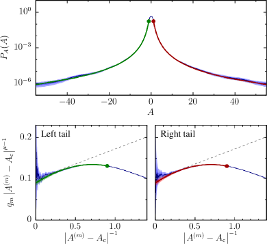
Figure 4: Application of the tail-regression procedure to a sample of $10^{6}$ random variables distributed according to $P_{A}(A)=\frac{1}{2}H_{3.1}(A)+\frac{1}{2}H_{4.1}(A)$. The top panel shows the estimated probability distribution, and the lower panels show $yx$ plots for each tail. Fits are shown as thick lines in the three panels, and the analytical asymptotic form of the tail is shown as a dashed line in each of the bottom panels. $68.3\%$ and $95.4\%$ confidence intervals obtained from the bootstrap are shown as shaded areas.

The regression of the tails of this model distribution is demonstrated in Fig. 4 using a sample of $10^{6}$ random variables. The top panel shows the probability distribution estimated by convolving the data with a variable-width Gaussian kernel, and the lower panels show $yx$ plots of the data. The tail fits are shown in the three panels as thick lines, for which we use $n_{\rm R}=3$ and $-\log q_{\rm R}=2.25$, and the constraint $c_{0}^{\rm L}=c_{0}^{\rm R}$ has been imposed.

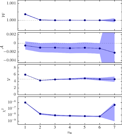
Figure 5: Tail-regression estimator of the zeroth, first, and second moment of $P_{A}(A)=\frac{1}{2}H_{3.1}(A)+\frac{1}{2}H_{4.1}(A)$ and $\chi^{2}$ as a function of expansion order obtained using a sample of $10^{6}$ random numbers and a threshold of $-\log q_{\rm R}=2.25$. The “optimal” $n_{\rm R}=3$ is that at which all of these functions reach their respective plateaus.

The process of selecting $n_{\rm R}$ at fixed threshold is illustrated in Fig. 5, where $\cal W$, $\cal A$, $\cal V$, and $\chi^{2}$ are plotted as a function of $n_{\rm R}$. These functions converge relatively quickly with $n_{\rm R}$, but for large expansion orders overfitting becomes an issue. This can be easily spotted by the significant jump in the uncertainty on the estimators, which in Fig. 5 occurs at $n_{\rm R}=7$. In this case we consider $n_{\rm R}=3$ to be the “optimal” expansion order.

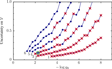
Figure 6: Uncertainty on the tail-regression estimator of $\sigma^{2}$ obtained from $10^{6}$ random variables distributed according to $P_{A}(A)=\frac{1}{2}H_{3.1}(A)+\frac{1}{2}H_{4.1}(A)$ as a function of threshold $-\log q_{\rm R}$. Each curve corresponds to a different expansion order $n_{\rm R}$, as labelled. Combinations of $-\log q_{\rm R}$ and $n_{\rm R}$ that fail to satisfy our correctness criteria are not shown, and narrow fails are shown as crossed-out points. The “optimal” choice of threshold and expansion order, marked with a circle, is that which minimizes the uncertainty on $\cal V$, corresponding to $-\log q_{\rm R}=2.25$ and $n_{\rm R}=3$ in this case.

In Fig. 6 we plot the uncertainty on $\cal V$ as a function of the threshold for each considered expansion order. The uncertainty on $\cal V$ is largely monotonic in $n_{\rm R}$ at fixed threshold and in $-\log q_{\rm R}$ at fixed expansion order. Figure 6 shows that the “optimal” values of the expansion order and threshold are $n_{\rm R}=3$ and $-\log q_{\rm R}=2.25$, as used in Fig. 4.

In Table 1 we report the results obtained from the standard and tail-regression estimators of $\langle A\rangle$ and $\sigma^{2}$ for sample sizes ranging from $10^{3}$ to $10^{8}$, which we plot in Figs. 7 and 8.

		Standard					TRE (unconstrained)							TRE (1 constraint)
$M$		$\bar{A}$		$S^{2}$			$n_{\rm R}$	$-\log q_{\rm R}$	$\cal A$		$\cal V$			$n_{\rm R}$	$-\log q_{\rm R}$	$\cal A$		$\cal V$
$10^{3}$		$0$.	$001(39)$	$1$.	$55(28)$		$1$	$3.25$	$0$.	$006(38)$	$3$.	$8(17)$		$5$	$1.00$	$0$.	$001(34)$	$3$.	$6(20)$
$10^{4}$		$-0$.	$000(18)$	$3$.	$3(13)$		$4$	$1.25$	$-0$.	$000(14)$	$2$.	$71(73)$		$3$	$1.50$	$0$.	$001(11)$	$3$.	$18(65)$
$10^{5}$		$0$.	$0009(50)$	$2$.	$51(31)$		$4$	$1.50$	$0$.	$0009(48)$	$4$.	$54(33)$		$4$	$1.50$	$0$.	$0057(35)$	$4$.	$55(33)$
$10^{6}$		$-0$.	$0017(16)$	$2$.	$63(19)$		$3$	$2.25$	$-0$.	$0014(15)$	$4$.	$57(12)$		$3$	$2.25$	$-0$.	$0011(11)$	$4$.	$56(12)$
$10^{7}$		$-0$.	$00022(52)$	$2$.	$69(12)$		$2$	$3.75$	$-0$.	$00017(46)$	$4$.	$585(41)$		$3$	$2.75$	$-0$.	$00032(37)$	$4$.	$608(49)$
$10^{8}$		$0$.	$00018(16)$	$2$.	$689(66)$		$3$	$2.75$	$0$.	$00016(15)$	$4$.	$661(15)$		$3$	$2.75$	$0$.	$00019(12)$	$4$.	$662(15)$
Exact		$0$.	$0$	$4$.	$6586$				$0$.	$0$	$4$.	$6586$				$0$.	$0$	$4$.	$6586$

Table 1: Standard and tail-regression estimators of $\langle A\rangle$ and $\sigma^{2}$ for model distribution $P_{A}(A)=\frac{1}{2}H_{3.1}(A)+\frac{1}{2}H_{4.1}(A)$ obtained from random samples of various sizes $M$. The “optimal” expansion orders $n_{\rm R}$ and thresholds $-\log q_{\rm R}$ used for the tail-regression estimator in each case are also shown.

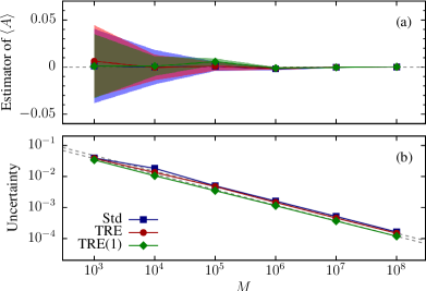
Figure 7: Convergence of (a) the estimators of $\langle A\rangle$ and (b) their uncertainties as a function of sample size $M$ for model distribution $P_{A}(A)=\frac{1}{2}H_{3.1}(A)+\frac{1}{2}H_{4.1}(A)$. The exact value $\langle A\rangle=0$ is marked with a dashed line in (a), and dashed lines proportional to $M^{-1/2}$ passing through the last point of each of the tail-regression estimator curves are shown in (b) as guides to the eye. $68.3\%$ confidence intervals are shown as shaded areas.

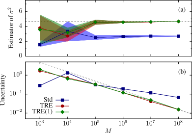
Figure 8: Convergence of (a) the estimators of $\sigma^{2}$ and (b) their uncertainties as a function of sample size $M$ for model distribution $P_{A}(A)=\frac{1}{2}H_{3.1}(A)+\frac{1}{2}H_{4.1}(A)$. The exact value $\sigma^{2}=4.6586$ is marked with a dashed line in (a), and dashed lines proportional to $M^{-1/2}$ passing through the last point of each of the tail-regression estimator curves are shown in (b) as guides to the eye. $68.3\%$ confidence intervals are shown as shaded areas.

For the tail-regression estimator we report results both without the use of constraints and imposing $c_{0}^{\rm L}=c_{0}^{\rm R}$. The “optimal” values of $n_{\rm R}$ and $-\log q_{\rm R}$ are not significantly sample-size dependent; we find that $n_{\rm R}$ increases when $-\log q_{\rm R}$ decreases and vice versa, as could be expected.

The estimators of $\langle A\rangle$ are within uncertainty of the exact value of zero at all sample sizes, but $\cal A$ has an uncertainty about $25\%$ smaller than $\bar{A}$. The uncertainty on the standard estimator of the variance $S^{2}$ is nonmonotonic, as expected, and in this case confidence interval sizes are severely underestimated, causing the false impression that $S^{2}$ converges to an incorrect value with increasing $M$. By contrast, $\cal V$ remains within uncertainty of $\sigma^{2}$ at all $M$, and its uncertainty decreases monotonically with sample size. The unconstrained and constrained estimators give indistinguishable results in this case, and the uncertainty on both seems to asymptotically decay as $M^{-1/2}$.

V.2 Distribution with undefined second moment

Distributions with $2<\mu\leq 3$ have a divergent variance, and the standard estimator of $\langle A\rangle$ has an undefined uncertainty. We exemplify this case with model distribution $P_{A}(A)=\frac{1}{2}H_{2.1}(A)+\frac{1}{2}H_{3.1}(A)$, which has $\mu=2.1$, close to the lower limit of $2$, and $\Delta=1$.

The standard and tail-regression estimators of $\langle A\rangle$ are given in Table 2 and plotted in Fig. 9 as a function of sample size $M$.

		Standard			TRE (unconstrained)					TRE (1 constraint)
$M$		$\bar{A}$			$n_{\rm R}$	$-\log q_{\rm R}$	$\cal A$			$n_{\rm R}$	$-\log q_{\rm R}$	$\cal A$
$10^{3}$		$-6$.	$4(67)$		$1$	$1.30$	$-0$.	$12(29)$		$1$	$1.60$	$-0$.	$026(43)$
$10^{4}$		$-0$.	$69(69)$		$5$	$1.00$	$-0$.	$11(20)$		$4$	$1.00$	$-0$.	$005(18)$
$10^{5}$		$0$.	$18(19)$		$5$	$1.10$	$0$.	$005(72)$		$6$	$1.00$	$-0$.	$0131(76)$
$10^{6}$		$-0$.	$21(17)$		$7$	$1.00$	$-0$.	$007(26)$		$4$	$1.40$	$-0$.	$0021(25)$
$10^{7}$		$-0$.	$115(66)$		$5$	$1.30$	$0$.	$0084(84)$		$4$	$1.50$	$0$.	$00073(83)$
$10^{8}$		$-0$.	$102(66)$		$4$	$1.70$	$0$.	$0028(28)$		$4$	$1.70$	$-0$.	$00003(29)$
Exact		$0$.	$0$				$0$.	$0$				$0$.	$0$

Table 2: Standard and tail-regression estimators of $\langle A\rangle$ for model distribution $P_{A}(A)=\frac{1}{2}H_{2.1}(A)+\frac{1}{2}H_{3.1}(A)$ obtained from random samples of various sizes $M$. The “optimal” expansion orders $n_{\rm R}$ and thresholds $-\log q_{\rm R}$ used for the tail-regression estimator in each case are also shown.

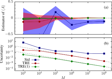
Figure 9: Convergence of (a) the estimators of $\langle A\rangle$ and (b) their uncertainties as a function of sample size $M$ for model distribution $P_{A}(A)=\frac{1}{2}H_{2.1}(A)+\frac{1}{2}H_{3.1}(A)$. The exact value $\langle A\rangle=0$ is marked with a dashed line in (a), and dashed lines proportional to $M^{-1/2}$ passing through the last point of each of the tail-regression estimator curves are shown in (b) as guides to the eye. $68.3\%$ confidence intervals are shown as shaded areas.

As expected, the standard estimator $\bar{A}$ hovers around the exact value $\langle A\rangle=0$ but its uncertainty does not decrease uniformly with sample size. The tail-regression estimator provides a monotonically decreasing uncertainty with an approximate asymptotic decay proportional to $M^{-1/2}$, and imposing the constraint $c_{0}^{\rm L}=c_{0}^{\rm R}$ yields an order of magnitude smaller uncertainties than the unconstrained estimator does.

V.3 Symmetric distribution with undefined first moment

Distributions with $1<\mu\leq 2$ have a divergent expectation value, and the standard estimator of $\langle A\rangle$ is undefined. However if the tails of the distribution are symmetric to leading order it is possible to redefine $\langle A\rangle$ as a Cauchy principal value which can be estimated, see Eq. 44. We exemplify this case with model distribution $P_{A}(A)=\frac{1}{2}H_{1.1}(A)+\frac{1}{2}H_{2.1}(A)$, which has $\mu=1.1$, close to the lower limit of $1$, and $\Delta=1$.

Results using the constrained tail-regression estimator are given in Table 3 and plotted in Fig. 10.

		Standard		TRE (1 constraint)
$M$		$|\bar{A}|$		$n_{\rm R}$	$-\log q_{\rm R}$	$\cal A$
$10^{3}$		$\sim 10^{30}$		$1$	$1.15$	$-0$.	$42(55)$
$10^{4}$		$\sim 10^{28}$		$2$	$0.95$	$0$.	$01(18)$
$10^{5}$		$\sim 10^{39}$		$2$	$1.00$	$0$.	$046(68)$
$10^{6}$		$\sim 10^{48}$		$3$	$1.10$	$-0$.	$028(54)$
$10^{7}$		$\sim 10^{59}$		$6$	$0.85$	$-0$.	$019(20)$
$10^{8}$		$\sim 10^{79}$		$5$	$0.95$	$-0$.	$0062(76)$
Exact		$0.0$				$0$.	$0$

Table 3: Standard and tail-regression estimators of $\langle A\rangle$ for model distribution $P_{A}(A)=\frac{1}{2}H_{1.1}(A)+\frac{1}{2}H_{2.1}(A)$ obtained from random samples of various sizes $M$. The “optimal” expansion orders $n_{\rm R}$ and thresholds $-\log q_{\rm R}$ used for the tail-regression estimator in each case are also shown.

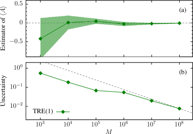
Figure 10: Convergence of (a) the constrained tail-regression estimator of $\langle A\rangle$ and (b) its uncertainty as a function of sample size $M$ for model distribution $P_{A}(A)=\frac{1}{2}H_{1.1}(A)+\frac{1}{2}H_{2.1}(A)$. The exact value $\langle A\rangle=0$ is marked with a dashed line in (a), and a dashed line proportional to $M^{-1/2}$ passing through the last point of the tail-regression estimator curve is shown in (b) as a guide to the eye. $68.3\%$ confidence intervals are shown as shaded areas.

We find that $\cal A$ is within uncertainty of the exact value of zero at all sample sizes, and again the uncertainty on $\cal A$ appears to be asymptotically proportional to $M^{-1/2}$. In Table 3 we also give the order of magnitude of the computed sample mean to highlight that this example is absolutely intractable with the standard estimator.

VI Application to variational quantum Monte Carlo data

In this section we explore the performance of the tail-regression estimator on data obtained from VMC calculations. Local values of observables generated using the VMC method are usually affected by serial correlation due to the use of the Metropolis algorithm to sample configuration space. In our VMC calculations we perform up to $400$ Metropolis steps between consecutive evaluations of the local values of the target observables so that these can be considered to be independent random variables, and we have verified that the resulting datasets exhibit negligible serial correlation.

VI.1 The energy of the homogeneous electron gas

The homogeneous electron gas is an ideal test bed for methodological developments in QMC. We perform VMC calculations on the paramagnetic 54-electron gas in a cubic simulation cell at density $r_{\rm s}=1$ using the Slater-Jastrow (SJ) wave function, consisting of the product of up- and down-spin Slater determinants of the plane-waves with the smallest momenta compatible with the periodicity of the simulation cell multiplied by a Jastrow correlation factor, $\Psi_{\rm SJ}({\bf R})={\rm e}^{J({\bf R})}D_{\uparrow}({\bf R}_{\uparrow})D_{\downarrow}({\bf R}_{\downarrow})$. Our Jastrow factor consists of an isotropic electron-electron term of the Drummond-Towler-Needs form Drummond_Jastrow_2004 ; LopezRios_Jastrow_2012 . We use the casino code casino_reference to generate samples of local energies whose distribution, as detailed in section II.1, has left and right heavy tails of principal exponent $\mu=4$, $\Delta=1$, and equal left- and right-tail leading-order coefficients Trail_htail_2008 . As explained in section IV.6, constraints involving $c_{n}$ with $n\geq 1$ cannot be applied since $A_{0}$ is being approximated by $A_{\rm c}$.

		Standard					TRE (unconstrained)							TRE (1 constraint)
$M$		$\bar{A}$		$S^{2}$			$n_{\rm R}$	$-\log q_{\rm R}$	$\cal A$		$\cal V$			$n_{\rm R}$	$-\log q_{\rm R}$	$\cal A$		$\cal V$
$10^{3}$		$0$.	$53381(74)$	$0$.	$000542(34)$		$2$	$4.25$	$0$.	$5339(12)$	$0$.	$00090(30)$		$2$	$4.50$	$0$.	$53342(96)$	$0$.	$00095(17)$
$10^{4}$		$0$.	$53314(24)$	$0$.	$000581(13)$		$2$	$6.50$	$0$.	$53309(26)$	$0$.	$000646(40)$		$1$	$7.75$	$0$.	$53310(26)$	$0$.	$000627(28)$
$10^{5}$		$0$.	$532868(76)$	$0$.	$0005738(39)$		$1$	$8.00$	$0$.	$532863(78)$	$0$.	$0005843(61)$		$1$	$8.25$	$0$.	$532868(76)$	$0$.	$0005839(57)$
$10^{6}$		$0$.	$532820(24)$	$0$.	$0005804(44)$		$2$	$7.25$	$0$.	$532817(24)$	$0$.	$0005806(24)$		$2$	$7.25$	$0$.	$532815(24)$	$0$.	$0005805(24)$
$10^{7}$		$0$.	$5328407(76)$	$0$.	$0005761(15)$		$2$	$8.00$	$0$.	$5328396(76)$	$0$.	$00057618(82)$		$3$	$8.25$	$0$.	$5328396(76)$	$0$.	$0005763(12)$
$10^{8}$		$0$.	$5328500(24)$	$0$.	$00057442(31)$		$2$	$8.25$	$0$.	$5328500(24)$	$0$.	$00057545(25)$		$2$	$8.25$	$0$.	$5328499(24)$	$0$.	$00057545(24)$

Table 4: Standard and tail-regression estimators of $\langle A\rangle$ and $\sigma^{2}$ for the VMC energy of the 54-electron gas at $r_{\rm s}=1$ using the SJ wave function obtained from local energy samples of various sizes $M$. The “optimal” expansion order $n_{\rm R}$ and threshold $-\log q_{\rm R}$ used for the tail-regression estimator in each case are also shown.

In Fig. 12 we plot the probability distribution estimated from $10^{6}$ local energies, $yx$ plots of the tails, and the corresponding tail fits.

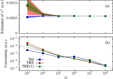
Figure 11: Convergence of (a) the estimators of $\sigma^{2}$ and (b) their uncertainties as a function of sample size $M$ for the VMC local energy of a 54-electron gas at $r_{\rm s}=1$ using the SJ wave function. Our best estimate of the value of the variance of the local energy for this system, $\sigma^{2}\approx 0.00057545(24)$ a.u., is marked with a dashed line in (a), and dashed lines proportional to $M^{-1/2}$ passing through the last point of each of the tail-regression estimator curves are shown in (b) as guides to the eye. $68.3\%$ confidence intervals are shown as shaded areas.

The standard and tail-regression estimators of $\langle A\rangle$ and $\sigma^{2}$, given in Table 4 and plotted in Fig. 11 as a function of sample size, are in good agreement with each other.

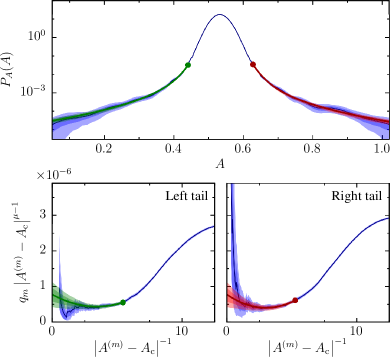
Figure 12: Application of the tail-regression procedure to a sample of $10^{6}$ VMC local energies for the 54-electron gas at $r_{\rm s}=1$ using the SJ wave function. The top panel shows the estimated probability distribution, and the lower panels show $yx$ plots of both tails. Fits are shown as thick lines in the three panels. $68.3\%$ and $95.4\%$ confidence intervals obtained from the bootstrap are shown as shaded areas.

The $\cal A$ estimator offers no advantage over $\bar{A}$ in this case, but the uncertainty on $S^{2}$ exhibits nonmonotonicity as a function of $M$, while that in $\cal V$ is monotonic, significantly smoother, and up to 45% smaller. Note that even though the nominal standard confidence interval on $S^{2}$ only shows minor signs of ill behavior in this example, it is formally undefined, while the tail-regression estimator produces valid confidence intervals. This is of potential practical importance in wave function optimization and variance extrapolation.

VI.2 The atomic force in the C₂ molecule

We turn our attention to the atomic force in the all-electron carbon dimer. The C₂ molecule is of particular interest due to its strong multi-reference character that makes the single-determinantal wave function incur a large nodal error, which ought to provide relatively strong heavy tails in the local Pulay and zero-variance force distributions.

We generate Hartree-Fock orbitals for the all-electron carbon dimer at an off-equilibrium (compressed) bond length of $r_{\rm CC}=2.0$ a.u. (the experimental equilibrium bond length of C₂ is $2.3481$ a.u. Toulouse_Umrigar_2008 ) using the relatively modest cc-pvdz basis set Dunning_basis_1992 ; Kendall_basis_1992 with the molpro code molpro . We combine these orbitals, modified to satisfy the Kato cusp conditions at electron-nucleus coalescence points Ma_cusp_2005 , with a Jastrow factor containing electron-electron, electron-nucleus, and electron-electron-nucleus terms of the Drummond-Towler-Needs form Drummond_Jastrow_2004 ; LopezRios_Jastrow_2012 , to form the trial wave function for VMC. Throughout the VMC run, performed with the casino code casino_reference , we collect local values of the components of the force on one of the carbon atoms along the molecular axis in the direction away from the other atom.

We first focus on the Pulay force which, as discussed in Section II.2, follows a heavy tailed distribution with $\mu=5/2$ and $\Delta=1/2$ due to the nodal error in the trial wave function. In Fig. 13 we show $yx$ plots of the tails of the local Pulay force at sample sizes $M=10^{6}$, $10^{7}$, and $10^{8}$, along with plots of the corresponding “optimal” fits.

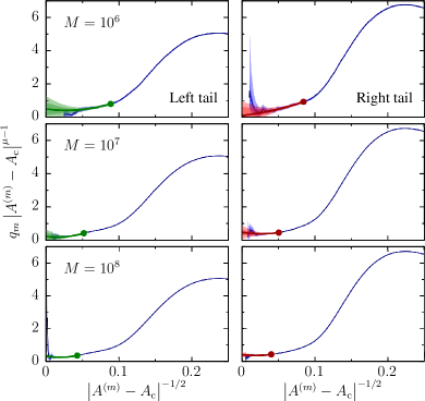
Figure 13: $yx$ plots of the left (left) and right (right) tails of the VMC local Pulay force on a carbon atom along the molecular axis of the C₂ molecule at $r_{\rm CC}=2$ a.u. at sample sizes $M=10^{6}$ (top), $10^{7}$ (middle), and $10^{8}$ (bottom). Fits are shown as thick lines in the three panels. $68.3\%$ and $95.4\%$ confidence intervals obtained from the bootstrap are shown as shaded areas.

Despite having chosen a system known to exhibit a large nodal error, we find that the leading-order heavy tails are relatively weak, and that it takes sample sizes of $M\gtrsim 10^{7}$ to resolve the nonzero value of $y(0)$. As a result, the uncertainty on the standard estimator of $\langle A\rangle$ is likely to only exhibit nonconvergent behavior at large sample sizes.

We plot the convergence of the standard and tail-regression estimators of $\langle F_{\rm P}\rangle$ in Fig. 14.

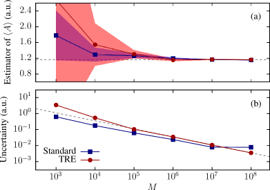
Figure 14: Convergence of (a) the estimators of $\langle A\rangle$ and (b) their uncertainties as a function of sample size $M$ for the VMC local Pulay force on a carbon atom along the molecular axis of the C₂ molecule at $r_{\rm CC}=2$ a.u.. The best value of the Pulay force of $1.1643(35)$ a.u. is marked with a dashed line in (a), and a dashed line proportional to $M^{-1/2}$ passing through the last point of the tail-regression estimator curve is shown in (b) as a guide to the eye. $68.3\%$ confidence intervals are shown as shaded areas.

As expected, the standard estimator $\bar{A}$ seems well behaved at small sample sizes, but at $M=10^{8}$ the standard error presents a substantial nonmonotonic jump. The uncertainty obtained with the tail-regression estimator remains smooth and monotonic, and is ultimately smaller than that of the standard estimator at $M=10^{8}$.

We find that the local zero-variance corrected Hellmann-Feynman force, $F_{\rm HFT}+F_{\rm ZV}$, and the local zero-variance corrected total force, $F_{\rm HFT}+F_{\rm P}+F_{\rm ZV}$, exhibit similarly weak leading-order tails, and the uncertainties in the standard and tail-regression estimators follow convergence patterns similar to those depicted in Fig. 14.

Without the zero-variance correction, the heavy tails affecting the distribution of the local Hellmann-Feynman force are very strong. As detailed in Section II.2, these tails are caused by the presence of all-electron nuclei and the left and right tails have equal leading-order coefficients. In Fig. 15 we plot the probability distribution of $F_{\rm HFT}$ for the off-equilibrium carbon dimer estimated from $10^{8}$ sample points and the corresponding $yx$ plots of the left and right tails of the distribution.

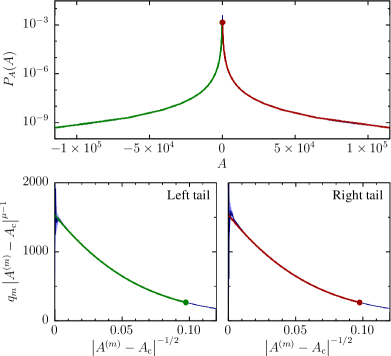
Figure 15: Application of the tail-regression procedure to a sample of $10^{8}$ VMC local Hellmann-Feynman forces on a carbon atom along the molecular axis of the C₂ molecule at $r_{\rm CC}=2$ a.u.. The top panel shows the estimated probability distribution, and the lower panels show $yx$ plots of both tails. Fits are shown as thick lines in the three panels. $68.3\%$ and $95.4\%$ confidence intervals obtained from the bootstrap are shown as shaded areas.

The value of $y(0)$ is very large relative to the rest of the function, and this is the only case among those we have considered in which the slope of the $yx$ plot is markedly negative at the origin. Indeed, it can be shown that the electron-nucleus cusp condition causes the $c_{1}$ coefficient in the asymptotic form of $F_{\rm HFT}$ to be approximately proportional to $c_{0}$ with a large, negative prefactor.

The standard and tail-regression estimators of the expectation value of the Hellmann-Feynman force are given in Table 5 and plotted in Fig. 16 as a function of sample size.

		Standard			TRE (unconstrained)					TRE (1 constraint)
$M$		$\bar{A}$			$n_{\rm R}$	$-\log q_{\rm R}$	$\cal A$			$n_{\rm R}$	$-\log q_{\rm R}$	$\cal A$
$10^{3}$		$-26$	$(56)$		$4$	$0.90$	$-18$	$(24)$		$3$	$0.90$	$0$	$.7(78)$
$10^{4}$		$-29$	$(22)$		$5$	$0.80$	$-3$	$.3(88)$		$4$	$0.90$	$-0$	$.7(33)$
$10^{5}$		$-2$	$.1(80)$		$5$	$0.80$	$0$	$.3(28)$		$5$	$0.80$	$0$	$.3(10)$
$10^{6}$		$-17$	$.0(73)$		$4$	$1.00$	$-0$	$.1(10)$		$4$	$1.00$	$-0$	$.34(40)$
$10^{7}$		$-8$	$.0(79)$		$3$	$1.30$	$-0$	$.43(34)$		$3$	$1.30$	$-0$	$.50(13)$
$10^{8}$		$-0$	$.3(15)$		$3$	$1.40$	$-0$	$.51(11)$		$3$	$1.40$	$-0$	$.567(43)$
Best		$-0$	$.5770(29)$				$-0$	$.5770(29)$				$-0$	$.5770(29)$

Table 5: Standard and tail-regression estimators of $\langle A\rangle$ for the VMC Hellmann-Feynman force on a carbon atom along the molecular axis of the C₂ molecule at $r_{\rm CC}=2$ a.u., obtained from local force samples of various sizes $M$. The “optimal” expansion orders $n_{\rm R}$ and thresholds $-\log q_{\rm R}$ used for the tail-regression estimator in each case are also shown. The “best” value is provided for reference and corresponds to the tail-regression estimator of $\langle F_{\rm HFT}+F_{\rm ZV}\rangle$ using $10^{8}$ sample points.

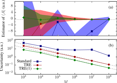
Figure 16: Convergence of (a) the estimators of $\langle A\rangle$ and (b) their uncertainties as a function of sample size $M$ for the VMC local Hellmann-Feynman force on a carbon atom along the molecular axis of the C₂ molecule at $r_{\rm CC}=2$ a.u.. The best value of the Hellmann-Feynman force of $-0.5758(29)$ a.u. is marked with a dashed line in (a), and dashed lines proportional to $M^{-1/2}$ passing through the last point of each of the tail-regression estimator curves are shown in (b) as guides to the eye. $68.3\%$ confidence intervals are shown as shaded areas.

The uncertainty on the standard estimator is clearly nonmonotonic, while that in the tail-regression estimator is smooth and appears to present an $M^{-1/2}$ asymptotic decay. The uncertainty on the tail-regression estimator is up to $60$ times smaller than the nominal uncertainty on the standard estimator, of which a factor of $2.5$ is thanks to imposing the analytical constraint $c_{0}^{\rm L}=c_{0}^{\rm R}$.

The results obtained for the different force components at the largest considered sample size of $M=10^{8}$ are given in Table 6.

	Standard		TRE		TRE(1)
$\langle F_{\rm HFT}\rangle$	$-0$	$.3(15)$	$-0$	$.51(11)$	$-0$	$.567(43)$
$\langle F_{\rm HFT}+F_{\rm ZV}\rangle$	$-0$	$.5731(42)$	$-0$	$.5770(29)$
$\langle F_{\rm P}\rangle$	$1$	$.1553(78)$	$1$	$.1643(35)$
$\langle F_{\rm HFT}+F_{\rm ZV}+F_{\rm P}\rangle$	$0$	$.5822(45)$	$0$	$.5860(35)$

Table 6: Standard and tail-regression estimators of $\langle A\rangle$ for the VMC local Hellmann-Feynman force, zero-variance corrected Hellmann-Feynman force, Pulay force, and zero-variance corrected total force on a carbon atom along the molecular axis of the C₂ molecule at $r_{\rm CC}=2$ a.u., obtained from $10^{8}$ sample points.

The nominal uncertainty on the standard estimator of $\langle F_{\rm HFT}+F_{\rm ZV}\rangle$ is an order of magnitude smaller than that in the constrained tail-regression estimator of $\langle F_{\rm HFT}\rangle$, and in this sense the tail-regression estimator is less effective than the zero-variance correction. This is however somewhat misleading since the uncertainty on the standard estimator remains formally ill-defined, while the tail-regression estimator is asymptotically normally distributed. In any case, the tail-regression estimator of $\langle F_{\rm HFT}+F_{\rm ZV}\rangle$ yields a $30\%$ lower uncertainty than the standard estimator, which is equivalent to a factor-of-two reduction in the number of sample points required to achieve a target uncertainty, showing that the combination of variance-reduction techniques with the tail-regression estimator is advantageous. Similarly, the nominal uncertainties on the Pulay force and on the zero-variance corrected total force are significantly reduced by replacing the ill-defined standard estimator with the tail-regression estimator at this sample size.

VII Application to diffusion quantum Monte Carlo data

At each post-equilibration step of a DMC calculation, an ensemble of walkers represents the mixed distribution $\Phi({\bf R})\Psi({\bf R})$, where $\Phi({\bf R})$ is the DMC wave function and $\Psi({\bf R})$ is the trial wave function. These walkers carry variable weights which in turn trigger death and branching events. The local values $\Psi^{-1}({\bf R})\hat{A}\Psi({\bf R})$ of an observable $\hat{A}$ are evaluated for each walker at each step, and the weighted average of the resulting sample yields the mixed estimator of the expectation value,

$$\langle A\rangle=\frac{\int\Phi({\bf R})\hat{A}\Psi({\bf R})\,{\rm d}{\bf R}}{\int\Phi({\bf R})\Psi({\bf R})\,{\rm d}{\bf R}}\;.$$ (45)

Note that one in principle seeks the pure estimator,

$$\langle A\rangle=\frac{\int\Phi({\bf R})\hat{A}\Phi({\bf R})\,{\rm d}{\bf R}}{\int\Phi({\bf R})\Phi({\bf R})\,{\rm d}{\bf R}}\;,$$ (46)

but the mixed estimator is simpler to obtain, it is equal to the pure estimator if $\hat{A}$ commutes with the Hamiltonian of the system, and for other observables there are ways of approximating pure estimators using mixed estimators Foulkes_QMC_2001 . We will restrict our discussion and tests to mixed estimators.

DMC samples differ from VMC samples in important ways. The formalism presented in section IV can be trivially altered to accommodate weights, simply by replacing the sample quantiles $q_{m}=\frac{m-1/2}{M}$ with

$$q_{m}=\frac{\sum_{l:A_{l}\geq A_{m}}p_{l}-p_{m}/2}{\sum_{l}p_{l}}\;,$$ (47)

where $p_{m}$ is the unnormalized weight of the $m$th sample point.

Walker branching events involve walkers being duplicated and its copies then evolving independently. This causes a complex pattern of serial correlation which cannot be eliminated entirely by leaving several steps between consecutive evaluations of the local values of observables, as we have done in our VMC calculations. While the presence of any form of serial correlation violates our assumption that samples consist of independent and identically distributed random variables, we expect this effect to be small and ignore it in our DMC tests.

The gradient of the DMC wave function $\Phi({\bf R})$ is in general discontinuous at the nodes Reynolds_dmc_1981 ; Moskowitz_lih_1982 . This alters the relative presence of walkers on either side of each nodal point, causing observables whose local values diverge at the nodes, such as the energy, to exhibit fully asymmetric heavy tails. The local Hellmann-Feynmann component of the force is not affected by this, since its singularities do not occur at the nodes of the trial wave function, so its DMC distribution remains symmetric to leading order as it is in VMC.

VII.1 The atomic force in the C₂ molecule

We have performed a DMC simulation of the C₂ molecule at the same off-equilibrium geometry and with the same wave function as described in Section VI.2, using a time step of $0.01$ a.u. Lee_strategies_2011 and a target population of $500$ walkers, and we have evaluated the local Hellmann-Feynmann and total forces for each walker every $5000$ steps.

The standard and tail-regression estimator of the Hellmann-Feynmann force are given in Table 7 and plotted in Fig. 17 as a function of sample size $M$. These results are very similar to their VMC counterparts; the nonmonotonic nominal standard error is again up to $60$ times the uncertainty in the tail-regression estimator, of which a factor of $2.5$ comes from imposing the constraint $c_{0}^{\rm L}=c_{0}^{\rm R}$.

		Standard			TRE (unconstrained)					TRE (1 constraint)
$M$		$\bar{A}$			$n_{\rm R}$	$-\log q_{\rm R}$	$\cal A$			$n_{\rm R}$	$-\log q_{\rm R}$	$\cal A$
$10^{3}$		$9$	$(35)$		$3$	$0.90$	$-14$	$(22)$		$3$	$1.10$	$-3$	$(11)$
$10^{4}$		$-29$	$(28)$		$5$	$0.80$	$-9$	$.5(87)$		$4$	$0.90$	$-3$	$.3(33)$
$10^{5}$		$4$	$.2(83)$		$4$	$0.90$	$-0$	$.3(28)$		$4$	$0.90$	$-0$	$.6(10)$
$10^{6}$		$6$	$.1(38)$		$3$	$1.40$	$0$	$.9(11)$		$3$	$1.40$	$0$	$.53(45)$
$10^{7}$		$-9$	$(12)$		$3$	$1.30$	$1$	$.08(34)$		$4$	$1.40$	$0$	$.61(18)$
$10^{8}$		$2$	$.5(29)$		$3$	$1.40$	$0$	$.41(11)$		$4$	$1.40$	$0$	$.306(58)$

Table 7: Standard and tail-regression estimators of $\langle A\rangle$ for the mixed DMC Hellmann-Feynman force on a carbon atom along the molecular axis of the C₂ molecule at $r_{\rm CC}=2$ a.u., obtained from local force samples of various sizes $M$. The “optimal” expansion orders $n_{\rm R}$ and thresholds $-\log q_{\rm R}$ used for the tail-regression estimator in each case are also shown.

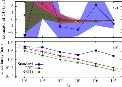
Figure 17: Convergence of (a) the estimators of $\langle A\rangle$ and (b) their uncertainties as a function of sample size $M$ for the mixed DMC local Hellmann-Feynman force on a carbon atom along the molecular axis of the C₂ molecule at $r_{\rm CC}=2$ a.u.. The best value of the Hellmann-Feynman force of $0.306(58)$ a.u. is marked with a dashed line in (a), and dashed lines proportional to $M^{-1/2}$ passing through the last point of each of the tail-regression estimator curves are shown in (b) as guides to the eye. $68.3\%$ confidence intervals are shown as shaded areas.

The results we obtain for the total force at the largest considered sample size of $M=10^{8}$ are given in Table 8. In this case, the uncertainty in the tail-regression estimator of the total force is $10\%$ smaller than the standard error.

	Standard		TRE		TRE(1)
$\langle F_{\rm HFT}\rangle$	$-2$	$.5(29)$	$-0$	$.41(11)$	$-0$	$.306(58)$
$\langle F_{\rm HFT}+F_{\rm ZV}+F_{\rm P}\rangle$	$0$	$.5810(42)$	$0$	$.5817(38)$

Table 8: Standard and tail-regression estimators of $\langle A\rangle$ for the mixed DMC local Hellmann-Feynman force and total force on a carbon atom along the molecular axis of the C₂ molecule at $r_{\rm CC}=2$ a.u., obtained from $10^{8}$ sample points.

From these tests we conclude that the tail-regression estimator is directly applicable to DMC samples generated using relatively long decorrelation loops, with essentially the same benefits as we have found for VMC samples.

VIII Conclusions

We have introduced a conceptually simple estimator of expectation values for heavy tailed probability distributions whose power-law tail indices are known. Unlike the standard estimator, the tail-regression estimator is immune to the breakdown of the central limit theorem for distributions of leading-order tail exponent $2<\mu\leq 3$. Our regression framework is designed to yield asymptotically normally distributed results, as reflected in the observed asymptotic $M^{-1/2}$ decay with sample size $M$ of the uncertainty in all of our tests, and successfully exploits known analytical relations between leading order tail coefficients to improve the estimation. We have also demonstrated the estimation of the variance of distributions of leading-order tail exponent $3<\mu\leq 5$ whose uncertainty is ill-defined under standard estimation.

Our tests of the tail-regression estimator with variational and diffusion quantum Monte Carlo data identifies two use cases of particular practical relevance. While the standard estimator yields accurate expectation values of the energy at large enough sample sizes, standard confidence intervals on the VMC variance of the local energy are formally undefined. The tail-regression estimator is capable of delivering valid confidence intervals on the variance which are up to $45\%$ smaller than those associated with the nominal standard error in our tests. The tail-regression estimator also yields valid, convergent confidence intervals on the VMC and DMC atomic force, including the Hellmann-Feynman force in all-electron systems for which we obtain uncertainties up to $60$ times smaller than the nominal standard error. The combination of the “zero-variance” variance-reduction technique with the tail-regression estimator yields accurate confidence intervals on the atomic force.

Our present work shows that the principles underpinning the tail-regression estimator are robust, and systematic use of the technique for treating quantum Monte Carlo data would be desirable. However, further work could improve the applicability of our present formulation. We have used the bootstrap to enable the evaluation of meaningful confidence intervals on a range of functions, but this approach should be replaced with the use of a closed expression for the uncertainty on the tail-regression estimator in production calculations. In turn, this would allow the development of an “on-the-fly” reformulation of the method that would avoid the need to store all local values of the desired observables, unaveraged, for later analysis. Dropping the requirement that sample points be independent and serially uncorrelated would also be desirable in order to reduce the computational cost of the QMC calculations. With these refinements, the tail-regression estimator will ultimately represent a great advance in ensuring the statistical soundness of results obtained from quantum Monte Carlo and similar methods.

Appendix A Tail-index estimation methods

Tail-index estimation methods draw inference on the principal exponent $\mu$ of a power-law heavy tail of leading-order form $P_{A}(A)=c_{0}A^{-\mu}$ at $A\to\infty$. The Hill estimator Hill_TIE_1975 of the first-order tail index, $\mu-1$, is

$$\frac{1}{\mu-1}\approx\frac{1}{M_{\rm R}}\sum_{m=1}^{M_{\rm R}}\log A^{(m)}-\log A^{(M_{\rm R}+1)}\;.$$ (48)

It can be shown that Eq. 48 is in fact equivalent to a logarithmic-scale least-squares fit to the tail of the distribution Beirlant_TIE_1996 . Substituting the leading-order form of $P_{A}(A)$ into Eq. 27 and taking logarithms yields

$$\log A^{(m)}\approx\frac{1}{\mu-1}\left(-\log q_{m}\right)+\frac{1}{\mu-1}\log\left(\frac{c_{0}}{\mu-1}\right)\;,$$ (49)

which is a linear relationship between $\log A^{(m)}$ and $-\log q_{m}$ with slope $\frac{1}{\mu-1}$. Estimation of this slope by linear regression following Eq. 49 yields Eq. 48 for the fitted slope if the $m$th data point is weighted by

$$w_{m}=\left(\log\frac{q_{M_{\rm R}+1}}{q_{m}}\right)^{-1}\;,$$ (50)

and $c_{0}$ is set so that the fit passes through the $(M_{\rm R}+1)$th point. The optimal value of $M_{\rm R}$ for the Hill estimator can thus be found by optimizing a goodness-of-fit measure with respect to $M_{\rm R}$ Beirlant_TIE_1996 , such as the $\chi^{2}$ value of the fit. Regression methods for tail-index estimation are found to be particularly robust Baek_TIE_2010 .

References

- (1) M. H. Kalos and P. A. Whitlock, Monte Carlo Methods (Wiley, New York, 1986).
- (2) H. Flyvbjerg and H. Petersen, Error estimates on averages of correlated data, J. Chem. Phys. 91, 461 (1989).
- (3) M. Jonsson, Standard error estimation by an automated blocking method, Phys. Rev. E 98, 043304 (2018).
- (4) D. W. Stroock, Probability Theory: An Analytic View (Cambridge University Press, Cambridge, England, 1993).
- (5) D. M. Ceperley and B. J. Alder, Ground State of the Electron Gas by a Stochastic Method, Phys. Rev. Lett. 45, 566 (1980).
- (6) W. M. C. Foulkes, L. Mitas, R. J. Needs, and G. Rajagopal, Quantum Monte Carlo simulations of Solids, Rev. Mod. Phys. 73, 33 (2001).
- (7) P. López Ríos, P. Seth, N. D. Drummond, and R. J. Needs, Framework for constructing generic Jastrow correlation factors, Phys. Rev. E 86, 036703 (2012).
- (8) P. López Ríos, A. Ma, N. D. Drummond, M. D. Towler, and R. J. Needs, Inhomogeneous backflow transformations in quantum Monte Carlo calculations, Phys. Rev. E 74, 066701 (2006).
- (9) M. Bajdich, L. Mitas, G. Drobný, L. K. Wagner, and K. E. Schmidt, Pfaffian Pairing Wave Functions in Electronic-Structure Quantum Monte Carlo Simulations, Phys. Rev. Lett. 96, 130201 (2006).
- (10) P. Seth, P. López Ríos, and R. J. Needs, Quantum Monte Carlo study of the first-row atoms and ions, J. Chem. Phys. 134, 084105 (2011).
- (11) N. D. Drummond, B. Monserrat, J. H. Lloyd-Williams, P. López Ríos, C. J. Pickard, and R. J. Needs, Quantum Monte Carlo study of the phase diagram of solid molecular hydrogen at extreme pressures, Nat. Commun. 6, 7794 (2015)
- (12) V. R. Pandharipande, S. C. Pieper, and R. B. Wiringa, Variational Monte Carlo calculations of ground states of liquid 4He and 3He drops, Phys. Rev. B 34, 4571 (1986).
- (13) J. R. Trail, Heavy-tailed random error in quantum Monte Carlo, Phys. Rev. E 77, 016703 (2008).
- (14) R. P. Feynman, Forces in Molecules, Phys. Rev. 56, 340 (1939).
- (15) P. Pulay, Ab initio calculation of force constants and equilibrium geometries in polyatomic molecules, Mol. Phys. 17, 197 (1969).
- (16) Mosé Casalegno, Massimo Mella, and Andrew M. Rappe, Computing accurate forces in quantum Monte Carlo using Pulay’s corrections and energy minimization, J. Chem. Phys. 118, 7193 (2003).
- (17) A. Badinski, P. D. Haynes, J. R. Trail, and R. J. Needs, Methods for calculating forces within quantum Monte Carlo simulations, J. Phys.: Condens. Matter 22 074202 (2010).
- (18) R. Assaraf and M. Caffarel, Zero-Variance Principle for Monte Carlo Algorithms, Phys. Rev. Lett. 83, 4682 (1999).
- (19) R. Assaraf and M. Caffarel, Computing forces with quantum Monte Carlo, J. Chem. Phys. 113, 4028 (2000).
- (20) R. Assaraf and M. Caffarel, Zero-variance zero-bias principle for observables in quantum Monte Carlo: Application to forces, J. Chem. Phys. 119, 10536 (2003).
- (21) M. C. Per, S. P. Russo, and I. K. Snook, Electron-nucleus cusp correction and forces in quantum Monte Carlo, J. Chem. Phys. 128, 114106 (2008).
- (22) A. Badinski, J. R. Trail, and R. J. Needs, Energy derivatives in quantum Monte Carlo involving the zero-variance property, J. Chem. Phys. 129, 224101 (2008).
- (23) A. Badinski and R. J. Needs, Accurate forces in quantum Monte Carlo calculations with nonlocal pseudopotentials, Phys. Rev. E 76, 036707 (2007).
- (24) A. Badinski and R. J. Needs, Total forces in the diffusion Monte Carlo method with nonlocal pseudopotentials, Phys. Rev. B 78, 035134 (2008).
- (25) S. Chiesa, D. M. Ceperley, and S. Zhang, Accurate, Efficient, and Simple Forces Computed with Quantum Monte Carlo Methods, Phys. Rev. Lett. 94, 036404 (2005).
- (26) C. Attaccalite and S. Sorella, Stable Liquid Hydrogen at High Pressure by a Novel Ab Initio Molecular-Dynamics Calculation, Phys. Rev. Lett. 100, 114501 (2008).
- (27) D. M. Hill, A Simple General Approach to Inference About the Tail of a Distribution, Ann. Stat. 3, 1163 (1975).
- (28) J. Beirlant, P. Vynckier, and J. L. Teugels, Tail Index Estimation, Pareto Quantile Plots Regression Diagnostics, JASA 91, 1659 (1996).
- (29) M. Kratz and S. I. Resnick, The qq-estimator and heavy tails, Comm. Statist. Stochastic Models 12, 699 (1996).
- (30) C. Baek and V. Pipiras, Estimation of parameters in heavy-tailed distribution when its second order tail parameter is known, J. Stat. Plan. Inference 140, 1957 (2010).
- (31) T. Kato, On the eigenfunctions of many-particle systems in quantum mechanics, Comm. Pure Appl. Math. 10, 151 (1957).
- (32) C. J. Umrigar, K. G. Wilson, and J. W. Wilkins, Optimized trial wave functions for quantum Monte Carlo calculations, Phys. Rev. Lett. 60, 1719 (1988).
- (33) M. Holzmann, D. M. Ceperley, C. Pierleoni, and K. Esler, Backflow correlations for the electron gas and metallic hydrogen, Phys. Rev. E 68, 046707 (2003).
- (34) A. Ma, M.D. Towler, N.D. Drummond, and R.J. Needs Scheme for adding electron-nucleus cusps to Gaussian orbitals, J. Chem. Phys. 122, 224322 (2005).
- (35) J. R. Trail and R. J. Needs, Correlated electron pseudopotentials for 3d-transition metals, J. Chem. Phys. 142, 064110 (2015).
- (36) J. R. Trail and R. J. Needs, Shape and energy consistent pseudopotentials for correlated electron systems, J. Chem. Phys. 146, 204107 (2017).
- (37) A. Badinski, Forces in Quantum Monte Carlo, PhD thesis, University of Cambridge (2008).
- (38) B. Efron and R. Tibshirani, Bootstrap Methods for Standard Errors, Confidence Intervals, and Other Measures of Statistical Accuracy, Stat. Sci. 1, 54 (1986).
- (39) N. D. Drummond, M. D. Towler, and R. J. Needs, Jastrow correlation factor for atoms, molecules, and solids, Phys. Rev. B 70, 235119 (2004).
- (40) R. J. Needs, M. D. Towler, N. D. Drummond, and P. López Ríos, Continuum variational and diffusion quantum Monte Carlo calculations, J. Phys.: Condens. Matter 22, 023201 (2010).
- (41) J. Toulouse and C. J. Umrigar, Full optimization of Jastrow-Slater wave functions with application to the first-row atoms and homonuclear diatomic molecules, J. Chem. Phys. 128, 174101 (2008).
- (42) T. H. Dunning Jr., Gaussian basis sets for use in correlated molecular calculations. I. The atoms boron through neon and hydrogen, J. Chem. Phys. 90, 1007 (1989).
- (43) R. K. Kendall, T. H. Dunning, and R. J. Harrison, Electron affinities of the first-row atoms revisited. Systematic basis sets and wave functions, J. Chem. Phys. 96, 6796 (1992).
- (44) H.-J. Werner, P. J. Knowles, G. Knizia, F. R. Manby, M. Schütz, P. Celani, W. Györffy, D. Kats, T. Korona, R. Lindh, A. Mitrushenkov, G. Rauhut, K. R. Shamasundar, T. B. Adler, R. D. Amos, A. Bernhardsson, A. Berning, D. L. Cooper, M. J. O. Deegan, A. J. Dobbyn et al., molpro version 2012.1, a package of ab initio programs, http://www.molpro.net.
- (45) P. J. Reynolds, D. M. Ceperley, B. J. Alder, and W. A. Lester, Fixed-node quantum Monte Carlo for molecules, J. Chem. Phys. 77, 5593 (1982).
- (46) J. W. Moskowitz, K. E. Schmidt, M. A. Lee, and M. H. Kalos, A new look at correlation energy in atomic and molecular systems. II. The application of the Green’s function Monte Carlo method to LiH, J. Chem. Phys. 77, 349 (1982).
- (47) R. M. Lee, G. J. Conduit, N. Nemec, P. López Ríos, and N. D. Drummond Strategies for improving the efficiency of quantum Monte Carlo calculations, Phys. Rev. E 83, 066706 (2011).
- (48) Our implementation of the tail-regression estimator can be found online at https://github.com/plopezrios/treat.