Software-Defined Design Space Exploration for an Efficient DNN Accelerator Architecture

Abstract

Deep neural networks (DNNs) have been shown to outperform conventional machine learning algorithms across a wide range of applications, e.g., image recognition, object detection, robotics, and natural language processing. However, the high computational complexity of DNNs often necessitates extremely fast and efficient hardware. The problem gets worse as the size of neural networks grows exponentially. As a result, customized hardware accelerators have been developed to accelerate DNN processing without sacrificing model accuracy. However, previous accelerator design studies have not fully considered the characteristics of the target applications, which may lead to sub-optimal architecture designs. On the other hand, new DNN models have been developed for better accuracy, but their compatibility with the underlying hardware accelerator is often overlooked. In this article, we propose an application-driven framework for architectural design space exploration of DNN accelerators. This framework is based on a hardware analytical model of individual DNN operations. It models the accelerator design task as a multi-dimensional optimization problem. We demonstrate that it can be efficaciously used in application-driven accelerator architecture design: we use the framework to optimize the accelerator configurations for eight representative DNNs and select the configuration with the highest geometric mean performance. The geometric mean performance improvement of the selected DNN configuration relative to the architectural configuration optimized only for each individual DNN ranges from 12.0% to 117.9%. Given a target DNN, the framework can generate efficient accelerator design solutions with optimized performance and area. Furthermore, we explore the opportunity to use the framework for accelerator configuration optimization under simultaneous diverse DNN applications. The framework is also capable of improving neural network models to best fit the underlying hardware resources. We demonstrate that it can be used to analyze the relationship between the operations of the target DNNs and the corresponding accelerator configurations, based on which the DNNs can be tuned for better processing efficiency on the given accelerator without sacrificing accuracy.

1 Introduction

Deep neural networks (DNNs) have recently become the fundamental inference vehicle for a broad range of artificial intelligence applications. Unlike conventional machine learning algorithms that rely on handcrafted features, DNNs extract features and learn the hidden patterns automatically from the training data. However, the superior performance of DNNs comes at the cost of requiring an immense amount of training data and massive computational complexity. The number of operations in the winning DNNs in the ImageNet Large Scale Visual Recognition Competition [1] has increased exponentially over the past few years, e.g., 1.4 GOPs for AlexNet [2] in 2012 to 38 GOPs for VGG-19 [3] in 2014. On the other hand, the slowdown of Moore’s Law scaling makes it difficult to keep pace with DNN growth, since the gap between the computational demand from DNNs and the computational capacity available from underlying hardware resources keeps increasing. Hence, specialized hardware architectures have been developed to efficiently process DNNs. DNNs map well to a graphical processing unit (GPU) due to its parallel architecture, massive number of computational units, and high memory bandwidth. However, GPU’s performance density, the computation capacity per unit area (floating-point operations per second/mm²), has almost saturated since 2011 [4]. The only improvement is due to technology scaling from 28 nm to 20 nm [4]. It is infeasible to continuously increase the chip area to accommodate larger DNNs without improving performance density.

Customized application-specific integrated circuits (ASICs)- and field-programmable gate array (FPGA)-based accelerators have also emerged for efficient DNN processing. These customized accelerators are designed to accelerate common low-level DNN operations, such as convolution and matrix multiplication. Hence, even though new DNN models are evolving rapidly and differ in their network architectures significantly, ASIC- and FPGA-based accelerators are still capable of processing various DNNs efficiently. FPGA-based accelerators [5, 6, 7, 8, 9, 10, 11, 12, 13] provide high parallelism and fast time-to-market. For example, an embedded FPGA platform is used as a convolver with dynamic-precision data quantization in [6] to achieve high throughput. In [7], a load-balance-aware pruning method is implemented on an FPGA to compress the long short-term memory (LSTM) model by 20$\times$. A dynamic programming algorithm is used to map DNNs to a deeply pipelined FPGA in [8]. It can achieve up to 21$\times$ and 2$\times$ energy efficiency relative to a central processing unit (CPU) and GPU, respectively. To avoid the long latency of the external memory access, an FPGA-based DNN accelerator is developed in [14] that keeps all the weigths and activations in the on-chip buffer. Alternatively, ASIC-based accelerators [15, 16, 17, 18, 19, 20, 21, 22, 23, 24] demonstrate much better power efficiency for DNN processing relative to general-purpose processors. For example, a model compression method is utilized in [15], where the inference engine can process the compressed network model efficiently through acceleration on sparse matrix-vector multiplications. A custom multi-chip machine-learning architecture, called DaDianNao, is presented in [17]. With each chip implemented as a single-instruction multiple-data (SIMD)-like processor, DaDianNao achieves two orders of magnitude speedup over a GPU. In [16], an ASIC accelerator is proposed for DNN training on the server end. It uses heterogeneous processing tiles with a low-overhead synchronization mechanism. A Fast Fourier Transform-based fast convolution is used in [25] to speed up convolutional layers, where convolutions are converted into matrix multiplications. Multiple convolutional layers are fused and processed in [26] to keep the intermediate data in the on-chip buffer, avoiding accesses to the external memory. The Google tensor processing unit (TPU) speeds up DNN inference with its multiply-accumulate (MAC) units arranged in a systolic structure [18]. It has extended support for DNN training in its second version. A row-stationary scheme, a dataflow used to minimize data movement, is proposed in [27] for a spatial accelerator architecture.

To improve accelerator performance density, the computational resources should be fully utilized using an efficient dataflow. Since convolutional layers typically constitute over 90% of total DNN operations [2, 28], parallelizing convolution computations can accelerate overall DNN processing significantly. The design space for convolutional layer processing comprises processing of multiple loops and data partitioning choices governed by limited on-chip memory [29]. In order to efficiently process the convolutional layer, loop unrolling, loop tiling, and loop interchange are often used in recent DNN accelerators [30, 29]. Compared to fast DNN model evolution, hardware accelerator implementations are much slower. Several systematic design space exploration methods have been proposed in order to bridge this gap [31, 32, 33]. However, previous accelerator designs do not fully consider the target applications in the early design stage. This may lead to the choice of a sub-optimal design from the DNN accelerator design space for the target applications since the characteristics of different DNNs may vary significantly and require very different architectural designs for efficient processing.

In this article, we make the following contributions:
1) We develop an application-driven framework for architectural design space exploration of efficient DNN accelerators. This framework is based on a hardware analytical model for various DNN operations. The design space exploration task is modeled as a multi-dimensional optimization problem, which can be handled using a genetic algorithm.
2) We use this framework in the early accelerator architecture design stage to achieve geometric mean performance improvements ranging from 12.0% to 117.9%.
3) We use this framework to explore optimization opportunities for simultaneously addressing diverse DNN applications.
4) We perform a sensitivity study of the relationship between DNN characteristics and the corresponding accelerator design configurations.

The rest of the article is organized as follows. Section 2 discusses background information on DNNs. Section 3 presents our hardware analytical model for DNN operations. Section 4 describes the application-driven framework for efficient accelerator design space exploration. Section 5 presents experimental results obtained by our framework on accelerator optimization and sensitivity study of DNN characteristics. Section 6 discusses the limitations of our framework and describes some potential future work. Section 7 concludes the article.

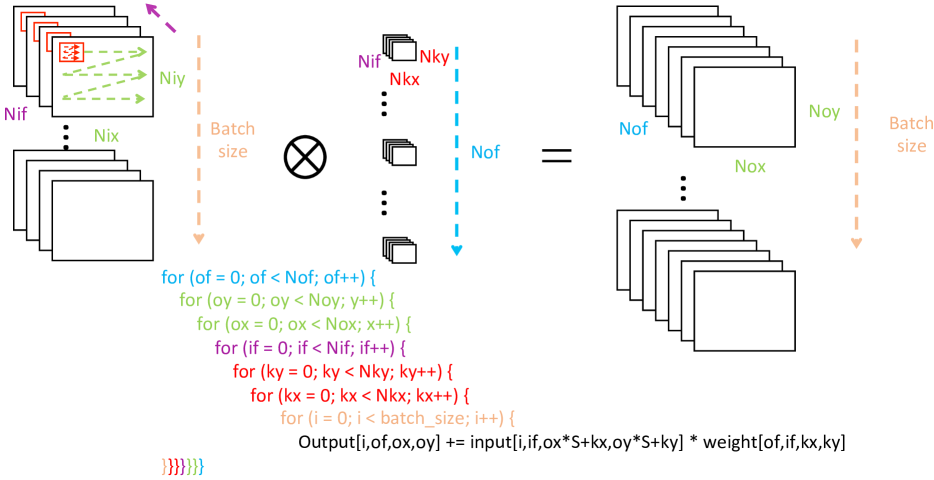
Figure 1: Convolutional layer of a DNN [29]

2 Background

In this section, we present background material to help understand the rest of the article. We first describe the convolutional layer of a DNN in Section 2.1. We then explore two optimization strategies used for DNNs: computational parallelism and data reuse, in Section 2.2 and Section 2.3, respectively.

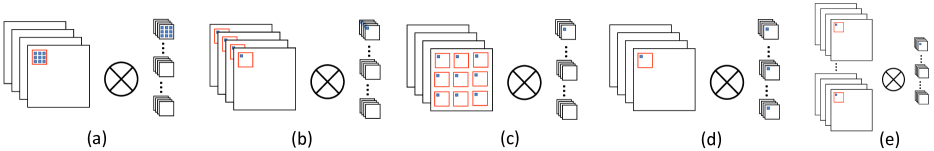
Figure 2: Loop unrolling [29]: (a) within one kernel window, (b) across input feature map channels, (c) within one input feature map, (d) across output feature map channels, and (e) across inputs in a batch

2.1 Convolutional layer of a DNN

The convolutional layer is one of the DNN building blocks. In the forward pass, the convolutional layer convolves a batch of 3D input feature maps with multiple learnable 3D kernel weights to generate a batch of 3D output feature maps. These learnable 3D kernel weights are trained to detect which features, such as edges, are present in the input feature maps. They also capture spatial and temporal dependencies in the input feature maps. As shown in Fig. 1, the convolutional layer operations can be represented by five sets of convolution loops: looping through different kernels, looping within one input feature map channel, looping through multiple input feature map channels, looping within one kernel channel, and looping through different inputs in the batch. The execution order of these loops can be interchanged to optimize the dataflow. N$of$, N$oy$, N$ox$, N$if$, N$ky$, N$kx$, batch_size, and S denote the number of output feature map channels, height and width of the output feature map, number of input feature map channels, height and width of the kernel window, input batch size, and sliding stride, respectively. These parameters are determined by the architecture of the DNNs. The on-chip memory of the accelerator may not be large enough to hold the entire data set for input feature maps, kernel weights, and output feature maps. Therefore, they need to be partitioned into smaller data chunks in order to fit in the on-chip memory. This is called loop tiling [30]. T* parameters (e.g., T$of$) denote the corresponding design variables for loop tiling. They represent the size of the data chunks stored in on-chip memory. Computational parallelism in the convolutional layer comes from loop unrolling, which increases the acceleration throughput and resource utilization ratio. P* parameters denote the number of parallel computations in each dimension. As the computing resources can only process data stored in an on-chip memory and the tiled data set is a subset of the total data set, the design constraints are set as P* $\leq$ T* $\leq$ N*. For instance, P$if\leq$ T$if\leq$ N$if$. The computational parallelism enabled by loop unrolling is discussed next.

2.2 Computational parallelism

Fig. 2(a)-(e) depict how the five types of loop unrolling work in the convolutional layer. Fig. 2(a) depicts loop unrolling within one kernel window. In each cycle, P$kx\times$P$ky$ input pixels and kernel weights in the kernel window are read in from the on-chip memory to perform parallel multiplications followed by P$kx\times$P$ky-1$ additions. The result is then added to the previously obtained partial sum. However, as the kernel sizes (N$kx$ and N$ky$) are usually relatively small, stand-alone loop unrolling within one kernel window cannot provide enough parallelism to fully utilize the accelerator compute resources [34]. Fig. 2(b) depicts loop unrolling across multiple input feature map channels. In each cycle, pixels at the same position in different channels are multiplied with the corresponding kernel weights across channels to produce P$if$ products. Then these products are summed up and accumulated with the partial sum. Fig. 2(c) shows loop unrolling within one input feature map channel. P$ix\times$P$iy$ input pixels are multiplied with the same kernel weight in parallel. The products are then accumulated to the corresponding partial sums in parallel. The input feature map sizes (N$ix$ and N$iy$) are typically large enough to provide sufficient parallelism for the accelerator as long as the required data are stored in the on-chip memory. Fig. 2(d) describes loop unrolling across different kernels. Multiple kernel weights at the same location from different kernels are multiplied with the same input pixels. The products are accumulated to the corresponding partial sums for different output feature map channels. Fig. 2(e) presents loop unrolling across inputs in the batch. Multiple inputs can be processed in parallel since there is no data dependency among them. These loop unrolling types can be combined to further increase the parallelism in convolutional layer processing. For example, loop unrolling within the kernel window, across multiple input feature map channels, and across different kernels are employed together in [6, 35, 34] while loop unrolling within one kernel window and within one input feature map channel are utilized in [27].

2.3 Data reuse

A convolutional layer is processed by sliding the kernel windows along the 3D input feature maps where MAC operations are performed at each sliding step. Since memory access and data movement incur significant delay and energy overheads [27], data fetched from on-chip memory should be reused as much as possible before being discarded.

If the loops within an input feature map (Fig. 2(c)) are unrolled, each kernel weight is broadcast to multiply with P$ix\times$P$iy$ different input pixels in every cycle. Thus, it is reused P$ix\times$P$iy$ times. If multiple inputs in the batch are processed in parallel (Fig. 2(e)), the number of times the kernel weight is reused is equal to the batch size. If both types of loop unrolling are employed, the total number of times each kernel weight is reused is:

$$weight\_reuse=Pix\times Piy\times batch\_size$$ (1)

If loops across output feature map channels (Fig. 2(d)) are unrolled, then each input pixel is multiplied with multiple kernel weights from different kernels in parallel. Hence, each input pixel is reused P$of$ times. Besides, if both loops within a kernel window (Fig. 2(a)) and within an input feature map (Fig. 2(c)) are unrolled together, then the pixels in neighboring kernel windows partially overlap as long as the sliding stride is smaller than the kernel window size. This results in the average number of times each input pixel is reused being P$kx\times$P$ky\times$P$ix\times$P$iy$/(((P$ix-1$)S+P$kx$)((P$iy-1$)S+P$ky$)) since the overlapped pixels can be reused in the following cycle. Combining the three types of loop unrolling mentioned above results in the total number of times each input pixel is reused being [29]:

$$input\_reuse=\frac{Pof\times Pkx\times Pky\times Pix\times Piy}{((Pix-1)S+Pkx)((Piy-1)S+Pky)}$$ (2)

3 Analysis of DNN operation processing

In this section, we provide an analysis of hardware accelerator processing of DNN operations. We extend the analytical model for 2D convolution discussed in [29] with batch processing enabled. Based on this approach, we build analytical models for various compute-intensive DNN operations.

The number of MAC operations in the convolutional layer is N_MAC = N$if\times$N$kx\times$N$ky\times$N$ox\times$N$oy\times$N$of$. Ideally, the total number of cycles required is N${}_{MAC}/$P_MAC, where P_MAC is the total number of the MAC units and assuming 100% MAC units efficiency. However, the available MAC units may not be fully utilized due to loop unrolling and loop tiling. In [29], the compute latency of the convolutional layer is modeled as the product of inter-tiling cycle and inner-tiling latency, where

$$\begin{multlined}inter\_tiling\_cycle=\\ \lceil\frac{Nif}{Tif}\rceil\lceil\frac{Nkx}{Tkx}\rceil\lceil\frac{Nky}{Tky}\rceil\lceil\frac{Nox}{Tox}\rceil\lceil\frac{Noy}{Toy}\rceil\lceil\frac{Nof}{Tof}\rceil\end{multlined}inter\_tiling\_cycle=\\ \lceil\frac{Nif}{Tif}\rceil\lceil\frac{Nkx}{Tkx}\rceil\lceil\frac{Nky}{Tky}\rceil\lceil\frac{Nox}{Tox}\rceil\lceil\frac{Noy}{Toy}\rceil\lceil\frac{Nof}{Tof}\rceil$$ (3)

$$\begin{multlined}inner\_tiling\_latency=\\ \lceil\frac{Tif}{Pif}\rceil\lceil\frac{Tkx}{Pkx}\rceil\lceil\frac{Tky}{Pky}\rceil\lceil\frac{Tox}{Pox}\rceil\lceil\frac{Toy}{Poy}\rceil\lceil\frac{Tof}{Pof}\rceil\end{multlined}inner\_tiling\_latency=\\ \lceil\frac{Tif}{Pif}\rceil\lceil\frac{Tkx}{Pkx}\rceil\lceil\frac{Tky}{Pky}\rceil\lceil\frac{Tox}{Pox}\rceil\lceil\frac{Toy}{Poy}\rceil\lceil\frac{Tof}{Pof}\rceil$$ (4)

Inter-tiling cycle refers to the number of data chunks used in loop tiling and inner-tiling latency refers to the number of cycles required to process each chunk. Memory transfer latency is modeled as the maximum of input memory cycles and weight memory cycles, where

$$num\_weight=Nox\times Noy\times Nkx\times Nky\times Nif\times Nof$$ (5)

$$\begin{multlined}num\_input=\\ Nox\times Noy\times Nkx\times Nky\times Nif\times Nof\times batch\_size\end{multlined}num\_input=\\ Nox\times Noy\times Nkx\times Nky\times Nif\times Nof\times batch\_size$$ (6)

$$weight\_cycles=\lceil\frac{num\_weight}{weight\_reuse\times weight\_bandwidth}\rceil$$ (7)

$$input\_cycles=\lceil\frac{num\_input}{input\_reuse\times input\_bandwidth}\rceil$$ (8)

With the assumption that memory bandwidth is not a bottleneck and multipliers can receive the input pixels and kernel weights continuously without incurring an idle cycle, the total processing latency for the convolutional layer is equal to the maximum value of the compute and memory transfer latencies.

To relax the constraint imposed by the memory bandwidth assumption made above and increase performance estimation accuracy, an extra optional finer-grained buffer simulator has been developed to monitor on-chip data. This on-chip buffer simulator estimates the memory transfer latency when the entire dynamic state of the DNN model cannot be held in the on-chip buffer. The entire convolutional layer is divided into multiple computational blocks that can be executed in parallel. Apart from the execution latency of each computational block, the memory transfer latency is also included if the data required by the block are not stored in the buffer. This buffer simulator simulates data fetching from and storing back to off-chip memory. The number of computational blocks represents a tradeoff between estimation speed and accuracy.

Depthwise separable convolution [36] is a variation of 2D convolution. It splits ordinary 2D convolution into two parts: 2D convolution within each channel (depthwise convolution) and mixing the channels using a set of 1$\times$1 convolutions across channels (channel mixing). Compared to ordinary convolution, it has fewer parameters. Therefore, it requires less computation and is less prone to overfitting. As shown in Table I, the first part, depthwise convolution, can be fit into the 2D convolution model discussed above with the number of filter kernels being equal to 1. The second part, channel mixing, can be fit into the 2D convolution model with 1$\times$1 kernel size.

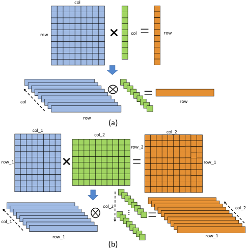
Figure 3: Model transformations of matrix-vector and matrix-matrix multiplications

Another important layer in a DNN is the fully-connected layer, which is processed as matrix-vector multiplication. We embed matrix-vector multiplication into 2D convolution to fit it into the analytical model described above, as shown in Fig. 3(a). The width, height, and depth of the input feature map are equal to the row number of the matrix, 1, and the column number of the matrix, respectively. The vector is transferred to the 1$\times$1 kernel with a depth equal to the matrix column number. Similarly, matrix-matrix multiplication is embedded into 2D convolution, as shown in Fig. 3(b). The second matrix is transferred to $col\_2$ 1$\times$1 kernels, where $col\_2$ is the column number of the second matrix. Details of the design parameter values used to fit depthwise separable convolution (depthwise convolution and channel mixing), matrix-vector multiplication, and matrix-matrix multiplication operations into the 2D convolution cost model are shown in Table I. In matrix-vector multiplication, col and row depict the matrix column number and row number, respectively. In matrix-matrix multiplication, col_1, row_1, and col_2 depict the column and row numbers of the first matrix, and column number of the second matrix, respectively.

TABLE I: Operation parameter values used in the cost model

2D conv.	Nif	Nix	Niy	Nkx	Nky	Nof	Nox	Noy	S
Depthwise conv.	Nif	Nix	Niy	Nkx	Nky	1	Nox	Noy	S
Channel mixing	Nif	Nix	Niy	1	1	Nof	Nox	Noy	S
Matrix-vector mul.	col.	row	1	1	1	1	row	1	1
Matrix-matrix mul.	col_1	row_1	1	1	1	col_2	row_1	1	1

TABLE II: Model validation with respect to an FPGA accelerator [29]

FPGA	Frequency	Actual	Estimated	Error
	(MHz)	latency (ms)	latency (ms)
Arria-10 GX 1150	150	47.97	38.73	19.3%

We validated these DNN operation analytical models against the FPGA accelerator proposed in [29] on VGG [3]. As shown in Table II, the error range is within 20%.

4 Application-driven architectural optimization

In this section, we discuss the proposed application-driven architectural optimization framework that is based on the analytical operation models.

4.1 Architectural optimization flow

Fig. 4 shows the accelerator architectural optimization flow. An architecture description file is used to define the design variables of the hardware accelerator. For example, it defines variables for the compute resource organization and the allocation of on-chip memory for activations and weights. Another input is the DNN computation graph of the target application that the accelerator is optimized for. We obtain this DNN computation graph by parsing the model file frozen from TensorFlow [37]. It is a directed acyclic graph (DAG) in which a vertex represents a DNN operation and an edge defines data dependency. The computation graph is first analyzed by a graph analyzer to generate a DNN operation stream. Then the latency of each operation in the stream is estimated using the cost model discussed in Section 3. The total latency of the DNN model is estimated as the sum of these latencies. We only focus on the time-consuming operations. Accelerator performance on the target application is then optimized using a multidimensional optimizer to obtain an optimized architectural configuration. The graph analyzer and the multidimensional optimizer are discussed in the following sections.

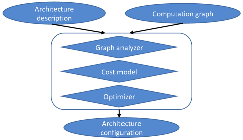
Figure 4: Architectural optimization flow

4.2 Computation graph analyzer

The graph analyzer is used to transfer the model graph into a stream of operations, where the model execution is assumed to follow the order of the stream and the latency of the operations can be estimated using the cost models discussed in Section 3. The DNN DAG is analyzed by performing depth-first search backward from the end node. The operation stream is obtained such that an operation can only be appended to the stream if it has no parent node or all of its parent nodes are already processed and are in the stream. The dynamic memory demand of the model is monitored during DAG traversal.

Fig. 5(a)-(d) show an example of a DAG and dynamic memory allocation analysis of the intermediate results. White nodes represent unprocessed operations that can only be processed if they have no parent nodes or all of their parent nodes have been processed. Then they become blue nodes whose outputs are stored in the on-chip memory. Their incoming edges are then removed since data dependency no longer exists after they are processed. A blue node turns to grey if it has no more outgoing edges, which means no more nodes depend on it. Hence, the memory space for its outputs can be deallocated. Dynamic memory allocation is monitored throughout DAG traversal and the maximum dynamic memory demand sets the lower bound for the on-chip buffer size of the accelerator if all the intermediate outputs (activations) need to be stored in the on-chip buffer.

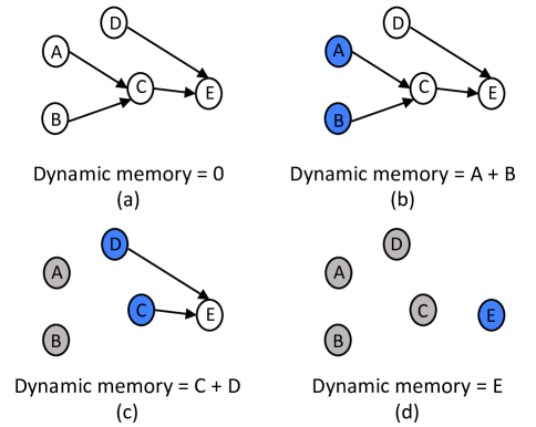
Figure 5: Illustration of dynamic memory allocation analysis

TABLE III: Accelerator architecture design variables

Variable name	Definition
loop_order	The execution order of the convolutional loops
PE_group	The total number of processing-element (PE) groups
MAC/group	The number of multiply-accumulates (MACs) in each PE group
buffer_bank_height	The height of the buffer bank
buffer_bank_width	The width of the buffer bank
weight_bank/group	The number of buffer banks per PE group for weights
activation_bank/group	The number of buffer banks per PE group for activations
Tif	The number of input feature map channels in loop tiling
Tix	The width of input feature map in loop tiling
Tiy	The height of input feature map in loop tiling
Tof	The number of output feature map channels in loop tiling

4.3 Multidimensional optimization

We model the architectural optimization task as a multidimensional optimization problem. We choose performance under an area constraint as our optimization metric, where the DNN processing latency is estimated from the analytical model described above. The design variables defined in the architecture description file are the independent variables for multidimensional optimization. Table III shows some of these variables. The minimum number of MAC units is constrained by the required number of parallel MAC operations per cycle:

$$\begin{multlined}PE\_group\times MAC/group\geq\\ Pox\times Poy\times Pkx\times Pky\times Pif\times Pof\end{multlined}PE\_group\times MAC/group\geq\\ Pox\times Poy\times Pkx\times Pky\times Pif\times Pof$$ (9)

The weight buffer size needs to be large enough to hold weight tiles. The maximum dynamic weight demand obtained from the computation graph analyzer sets the lower bound:

$$weight\_buffer\geq Tkx\times Tky\times Tif\times Tof\times bit\_width$$ (10)

$$weight\_buffer\geq peak\_weight\_memory\_demand$$ (11)

Similarly, the constraints on the activation buffer size are:

$$\begin{multlined}activation\_buffer\geq\\ (Tix\times Tiy\times Tif+Tox\times Toy\times Tof)\times bit\_width\end{multlined}activation\_buffer\geq\\ (Tix\times Tiy\times Tif+Tox\times Toy\times Tof)\times bit\_width$$ (12)

$$\begin{multlined}activation\_buffer\geq\\ peak\_input\_memory\_demand\times batch\_size\end{multlined}activation\_buffer\geq\\ peak\_input\_memory\_demand\times batch\_size$$ (13)

The $Tix\times Tiy\times Tif$ and $Tox\times Toy\times Tof$ products in Eq. 12 correspond to input feature map tiling and output feature map tiling, respectively.

The accelerator area is estimated under the assumption of unit area for each component, e.g., MAC, control logic, on-chip buffer, and register file. The total area is then scaled according to the architectural configuration.

We use a genetic algorithm [38] to solve the multidimensional optimization problem. Other optimization methods, such as integer linear programming, may also be used. The pseudocode of the genetic algorithm is shown in Algorithm 1, where $K$, $\alpha$, $\beta$, and $\gamma$ denote the total number of generations, the percentage of top configurations that will pass to the next generation, the range of top configurations in the current generation that will be selected as parents in the crossover operation, and the probability of mutation, respectively. The performance of an accelerator architecture configuration is used as the fitness score. During crossover, a list of configuration variables is randomly selected. The offspring are then generated by swapping the variable values inherited from the parents. During mutation, a list of configuration variables is randomly selected. Then the given configuration variable values are subjected to mutation. We start with $n$ random initial valid accelerator configurations in the first generation. In each iteration, we first sort the configurations based on their performance. The top $\alpha n$ configurations pass through to the next generation. Then, the remaining configurations are generated through crossover with parents from the top $\beta n$ configurations in the current generation. Finally, $\gamma n$ configurations go through the mutation process to increase diversity. This process repeats until the total number of generations is reached or the performance improvement converges.

Algorithm 1 Genetic algorithm

1:Start with $n$ random initial valid accelerator configurations as the initial generation $G_{0}$

2:for $i\leftarrow 0$ to $K-1$ do

3:     Sort $G_{i}$ based on their fitness scores

4:     $G_{i+1}\leftarrow G_{i}[0:\alpha n]$

5:     while $size(G_{i+1})<n$ do

6:         Randomly pick two numbers $f$ and $m$ in (0, $\beta n$)

7:         $F\leftarrow G_{i}[f]$

8:         $M\leftarrow G_{i}[m]$

9:         $G_{i+1}\leftarrow G_{i+1}+Crossover(F,M)$      

10:     Randomly select $\gamma n$ configurations $G_{m}$ in $G_{i+1}$

11:     $G_{m}\leftarrow Mutation(G_{m})$

5 Hardware-software co-design study

In this section, we study the relationship between the accelerator architecture and the characteristics of its target DNN applications based on the optimization framework. We first optimize accelerator performance under an area constraint on the target applications through accelerator design space exploration. We provide an analysis of the characteristics of the different optimized architectures. We then explore the optimization opportunities for the accelerator architecture when multiple diverse DNN applications run simultaneously. Finally, we study the relationships between DNN applications and the resulting optimized hardware accelerators.

5.1 Accelerator architecture design space exploration

We have selected eight representative DNNs: Inception-v3 (inception) [39], DeepLabv3 (deeplab) [40], ResNet-v1-50 (resnet) [41], Faster R-CNN (fasterRCNN) [42], PTB (ptb) [43], Wide & Deep Learning (wdl) [44], NASNet (nasnet) [45], and VGG16 (vgg) [3], and use the application-driven architectural optimization framework discussed in Section 4 to optimize the accelerator performance under an area constraint.

Inception-v3 is a convolutional neural network (CNN) that uses filters with multiple sizes in the same layer. Extra 1$\times$1 convolutions are added before 3$\times$3 and 5$\times$5 convolutions to reduce the number of input feature channels, and thus the computational complexity of the network. DeepLabv3 is a CNN aimed at semantic image segmentation. It assigns labels to every pixel of the input image. It is constructed based on ResNet-101 [41] and employs atrous spatial pyramid pooling for object segmentation at multiple scales. ResNet-v1-50 is a CNN that uses an “identity shortcut connection” to solve the vanishing gradient problem [46] during training. Faster R-CNN uses two networks for real-time object detection: a region proposal network for object boundary predictions and another network to detect objects in the bounding boxes. PTB is a recurrent neural network that uses LSTM units for word prediction. Wide & Deep Learning is a model for recommender systems. It jointly trains a wide linear model and a DNN for memorization and generalization, respectively. NASNet is a network that is automatically generated by AutoML, which automates the design of machine learning models. It searches for the best layers on CIFAR-10 [47] and transfers the architectures to ImageNet [1] for object detection. VGG16 is a convolutional neural network that replaces large kernel-sized filters in AlexNet with 3$\times$3 filters and stacks multiple convolutional layers on top of each other to increase depth and improve image recognition accuracy.

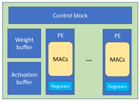
Figure 6: Architectural template of the accelerator

Fig. 6 shows a template of the accelerator architecture. Two on-chip buffers are used to store weights and activations, respectively, and MACs are distributed in multiple PE groups. We assume that the accelerator bit-width is 8 and that it uses a batch size of 4. We select the obtained architectural configurations with top 10% performance (in giga operations per second (GOPS)) for each DNN application as candidates for optimized configuration selection. Their design configurations are normalized for each variable and plotted in Fig. 7(a)-(h). Their performance on the eight DNN applications is shown in Fig. 8(a)-(h). The highest performance on each DNN is achieved by the architectural configuration optimized for that application using the framework. A configuration with 0 GOPS in Fig. 8 means that the architecture violates the constraints mentioned in Section 4.3 for that specific application.

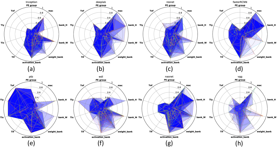
Figure 7: Radar charts of accelerator configurations with top 10% performance

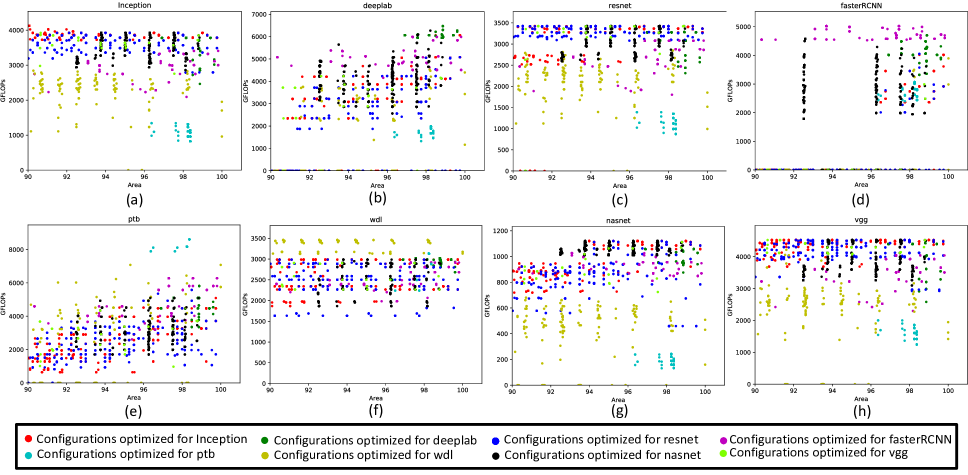
Figure 8: Performance on selected DNN applications of accelerator configurations with top 10% performance

TABLE IV: Summary of the selected DNNs

	inception	deeplab	resnet	fasterRCNN	ptb	wdl	nasnet	vgg
peak input memory demand	2.8MB	12.7MB	2.4MB	30.1MB	8.0MB	20.0KB	5.3MB	3.1MB
peak weight memory demand	2.1MB	12.8MB	2.4MB	0.3MB	2.0MB	8.0KB	0.2MB	2.0MB
#Conv2D layers	95	38	53	33	0	0	196	13
#Depthwise separable convolutions	0	17	0	13	0	0	160	0
#Matrix-matrix mul. layers	0	0	0	4	41	3	1	3

We can see that Fig. 7(a) and Fig. 7(c) have similar shapes. This means that the optimized architectures for Inception-v3 resemble those for ResNet-v1-50. This is consistent with the performance plots in Fig. 8(a) and Fig. 8(c), respectively, where they both achieve the highest performance on the two networks. The reason for this architecture and resulting performance similarities is that the two networks share similar characteristics, as shown in Table IV. Inception-v3 and ResNet-v1-50 have similar peak input/weight memory demands, which means that the two networks require similar on-chip buffer size for the same data processing batch. This is why Fig. 7(a) and Fig. 7(c) have the same values for bank height, bank width, #weight banks, and #activation banks. Besides, both networks mainly comprise 2D convolutional layers. Although the depths of the two networks are different, the distributions of the feature map size and the number of feature map channels are similar, as shown in Fig. 9 and Fig. 10, respectively. Architectures optimized for DeepLabv3 and Faster R-CNN also show similarity in terms of their architectural configurations (Fig. 7(b) and Fig. 7(d)) and performance on the two networks (Fig. 8(b) and Fig. 8(d)). They both require relatively larger on-chip memory for inputs. Therefore, there are dense horizontal lines at 0 GOPS level in Fig. 8(b) and Fig. 8(d) because these architectural configurations violate on-chip memory constraints.

Among all candidate configurations, we select the one with the highest geometric mean of performance on the eight DNNs. It is compared to the architectural configurations with the best performance on each individual DNN, as shown in Table V. The selected configuration outperforms the best configuration for each DNN by 12.0% to 117.9% in terms of geometric mean performance, as shown in Table VI. The different characteristics of various DNNs may lead to significantly different configurations in the design space. Thus, the target applications should be considered in the early design stage to design efficient accelerators for a broad range of DNN applications.

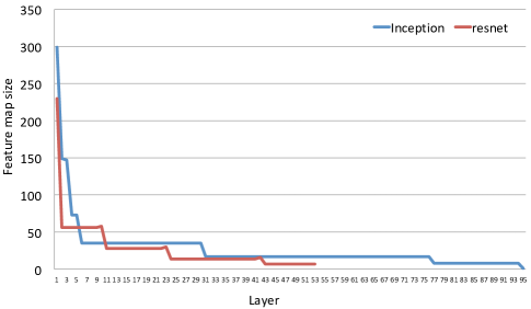
Figure 9: Feature map size comparisons of Inception-v3 and ResNet-v1-50

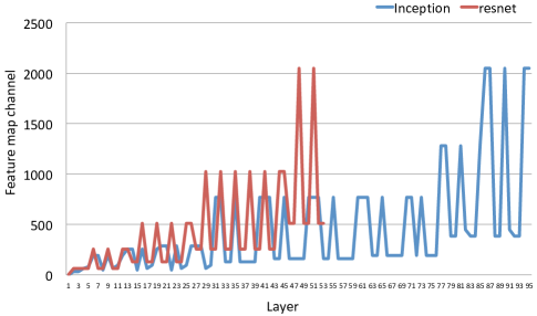
Figure 10: Feature map channel comparisons of Inception-v3 and ResNet-v1-50

TABLE V: Performance (GOPS) comparisons of the selected optimized configuration and the best configuration for each DNN. Performance on each DNN normalized to that of the best configuration

	Best on	Best on	Best on	Best on	Best on	Best on	Best on	Best on	Selected
	inception	deeplab	resnet	fasterRCNN	ptb	wdl	nasnet	vgg	optimized result
inception	1.00	0.73	0.98	0.76	0.27	0.59	0.99	0.98	0.94
deeplab	0.64	1.00	0.64	0.83	0.27	0.70	0.64	0.64	0.94
resnet	0.99	0.76	1.00	0.77	0.32	0.61	0.99	0.99	0.96
fasterRCNN	0.47	0.84	0.50	1.00	0.55	0.69	0.47	0.50	0.84
ptb	0.38	0.54	0.43	0.47	1.00	0.62	0.38	0.43	0.59
wdl	0.68	0.85	0.66	0.69	0.83	1.00	0.68	0.66	0.83
nasnet	0.99	0.86	0.99	0.89	0.17	0.46	1.00	0.99	0.94
vgg	0.99	0.71	0.99	0.78	0.35	0.56	0.99	1.00	0.98
Geometric mean	0.72	0.78	0.74	0.76	0.40	0.64	0.72	0.74	0.87

TABLE VI: Average performance improvements of the selected result over the best configuration for each DNN

Over the best	Over the best	Over the best	Over the best	Over the best	Over the best	Over the best	Over the best
on inception	on deeplab	on resnet	on fasterRCNN	on ptb	on wdl	on nasnet	on vgg
20.0%	12.0%	18.0%	14.8%	117.9%	36.1%	20.0%	18.0%

5.2 Multi-context optimization

From Fig. 7, we observe that the optimized accelerator architectures diverge for different DNN applications. Hence, in this section, we explore if there exist new optimization opportunities when very different DNN applications run simultaneously on the same hardware accelerator.

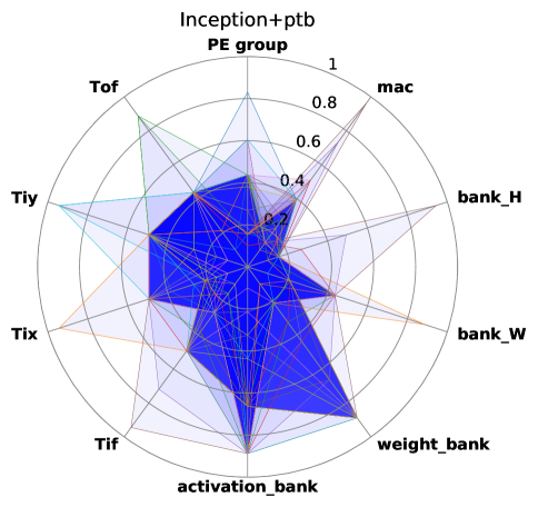
Figure 11: Radar chart of accelerator configurations for a multi-context application

First, we mix Inception-v3 and PTB by interleaving layers from both DNNs. Then, we use the framework to optimize the accelerator architecture on this mixed DNN in a multithreaded manner: the operations from Inception-v3 and PTB run on the accelerator alternately. The multithreading scenario is simplified using this mixed-layer stream. In real scenarios, a more sophisticated scheduler would be needed to decide the layer execution order for the two models. The inference results obtained using the multithreading mixed-layer stream are the same as when the two models are run back-to-back, as layers from different models are tagged and data are not shared across models.

Fig. 11 shows the resulting architectural configurations with top 10% performance on this multi-context application. This radar chart is quite different from those shown in Fig. 7(a) and Fig. 7(e) and is not a simple combination of those two radar charts. It has smaller #macs compared to Fig. 7(a) and smaller loop tiling sizes, e.g., $Tof$, $Tiy$, and $Tix$, relative to Fig. 7(e). As shown in Table IV, Inception-v3 is compute-intensive: it is dominated by 2D convolutional layers and thus requires relatively larger #macs for efficient processing. On the other hand, PTB is memory-intensive: it consists of a large number of matrix-matrix multiplication layers with relatively high peak input/weight demand. Hence, large tiling sizes appear in its optimized architectural configurations. However, when these two DNN applications run simultaneously on the same accelerator, the required amount of compute and memory resources is lowered in the optimized configurations. The reasons for this are two-fold. First, under an area constraint, the optimized architectural configurations for the multi-context application need to maintain a balance between compute and memory resources. Second, the complementary characteristics of Inception-v3 and PTB help relax both compute and memory design constraints on the accelerator architecture: while MACs are mainly devoted to convolutional layers of Inception-v3, filter weights can be transferred between the weight buffer and external memory for matrix-matrix multiplication layers for PTB at the same time, with no or very little performance loss, since the layers of both DNNs are interleaved. This shows that the optimal design for multi-context applications may not be a simple combination of designs optimized for the individual applications and new optimization opportunities can be explored using our application-driven architectural design space exploration framework.

5.3 Application sensitivity analysis

It is evident that the application-driven architectural optimization framework will generate similar architectural configurations for DNNs with common characteristics. However, to better understand the reasons for the different accelerator configuration results shown in Fig. 7, we perform an application sensitivity analysis to discover the hardware-software relationship in DNN applications.

We build the Faster R-CNN network in four steps. In the first step, we build a DNN with the same number of 2D convolutional layers as that in Faster R-CNN, but with relatively larger feature map sizes. The next step is to make the convolution dimensions the same as those in the Faster R-CNN. Depthwise separable convolutional layers and matrix-matrix multiplication layers are then added in the following two steps. In each step, we use the architectural optimization framework to generate the architectural configurations and select those with top 10% performance.

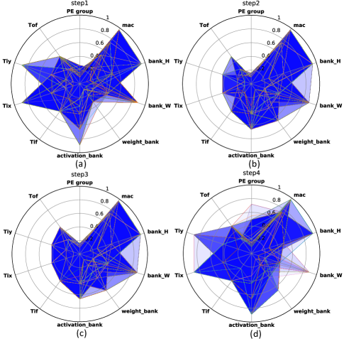
Figure 12: Radar charts of accelerator configurations at each step

Fig. 12(a)-(d) show the optimized architectural configurations obtained at each step. We can see that reducing the feature map sizes of the convolutional layers (from Fig. 12(a) to Fig. 12(b)) impacts the loop tiling design variables. Smaller tiling sizes are preferred for better performance. According to Eq. (3), reducing the feature map size while keeping loop tiling variables unchanged may lower the efficiency of memory transactions. Thus, the value of loop tiling variables is also reduced in Fig. 12(b). In the third step, 13 depthwise separable convolutional layers are inserted every two Conv2D layers with the same convolution dimensions as their following Conv2D layers. Comparing Fig. 12(b) and Fig. 12(c), we can see that just adding depthwise separable convolution operations without changing the feature map size does not affect the optimized architectural configurations. In the fourth step, large matrix multiplication layers are added. The number of PE groups is increased to generate more parallel MACs for matrix multiplication processing. Besides, this also increases the value of loop tiling variables again since more computational parallelism can be exploited when processing larger data chunks. This is consistent with the architectural configurations optimized for PTB, as shown in Fig. 7(e), where the network only consists of large matrix multiplication layers. Fig. 7(a)-(c) and Fig. 7(g)-(h) have small design variables in loop tiling dimensions since there are no matrix multiplication layers or the matrix dimension is small.

If the underlying hardware compute resource is fixed, we can perform a similar sensitivity analysis on the target network using this application-driven architectural optimization framework. The analysis results can guide DNN model development to fit the underlying compute resource.

6 Discussions and limitations

In this section, we discuss the assumptions we made in our framework and identify future work to tackle these limitations.

Similar to the designs in [6, 7, 48, 26], we assume the architectural template uses dedicated separate weight and activation on-chip buffers. However, there are other designs in which a unified memory is used for weights and activations. A future direction for improving our design space exploration framework is to support a unified memory design.

Another limitation of our memory modeling technique is that it does not model memory distribution across multiple PEs, hence overlooking data sharing and replication. A more accurate memory modeling technique is required for this purpose.

Since our analytical modeling framework is useful for early stage design space exploration, it is very sensitive to modeling latency in order to explore the huge design space. A more accurate architecture/memory modeling method may be too slow for early design space exploration. Therefore, a hierarchical modeling method could be used to obtain a balance between modeling accuracy and latency: a coarse-grained modeling method in the first step, where a small number of candidate configurations are selected, and a finer-grained modeling method applied in the second step to those selected configurations to obtain the final results. We leave this as future work.

7 Conclusion

In this article, we proposed an application-driven accelerator architectural optimization framework. This framework explores the accelerator design space and optimizes the architectural configuration for the target applications based on the analytical models. We use a genetic algorithm to solve the multi-dimensional optimization problem. We use this framework to optimize the accelerator architectural configuration for eight selected DNN applications. We show that the architectural configuration optimized for all the eight DNNs can achieve geometric mean performance improvements ranging from 12.0% to 117.9% over the configurations optimized only for each individual DNN. In addition, we explore the opportunity to use the framework for accelerator architectural configuration optimization when complementary DNN applications run simultaneously. Furthermore, the framework can be used to guide DNN model development for running on the fixed hardware accelerator more efficiently.

Ye Yu received the B.Eng. degree in Electronic and Computer Engineering from The Hong Kong University of Science and Technology, Hong Kong, China, in 2014, and the M.A. and Ph.D. degrees in Electrical Engineering from Princeton University, NJ, USA, in 2016 and 2019, respectively. He is currently a software engineer at Microsoft. His current research interests include computer vision, machine learning, deep learning model compression and acceleration.

Yingmin Li Yingmin Li received his B.S. in Computer Science from Zhejiang University, China and Ph.D. in Computer Science from University of Virginia. Yingmin is currently a senior staff engineer at Alibaba’s Infrastructure Services Group. His research interests include machine learning, performance optimization for heterogeneous systems, and computer architecture.

Shuai Che Shuai Che received the Ph.D. degree in Computer Engineering from the University of Virginia in 2012 and Bachelor of Engineering degree from Shanghai Jiaotong University in 2004. His research interests include computer architecture, heterogeneous computing, GPGPU, machine learning, and graph computing.

Niraj K. Jha (S’85-M’85-SM’93-F’98) received his B.Tech. degree in Electronics and Electrical Communication Engineering from Indian Institute of Technology, Kharagpur, India in 1981, M.S. degree in Electrical Engineering from S.U.N.Y. at Stony Brook, NY in 1982, and Ph.D. degree in Electrical Engineering from University of Illinois at Urbana-Champaign, IL in 1985. He is a Professor of Electrical Engineering at Princeton University. He has served as the Editor-in-Chief of IEEE Transactions on VLSI Systems and an Associate Editor of IEEE Transactions on Circuits and Systems I and II, IEEE Transactions on VLSI Systems, IEEE Transactions on Computer-Aided Design, IEEE Transactions on Computers, IEEE Transactions on Multi-Scale Computing System, Journal of Electronic Testing: Theory and Applications, and Journal of Nanotechnology. He is currently serving as an Associate Editor of Journal of Low Power Electronics. He has served as the Program Chairman of several conferences, the Director of the Center for Embedded System-on-a-chip Design funded by New Jersey Commission on Science and Technology, and the Associate Director of the Andlinger Center for Energy and the Environment. He is the recipient of the AT&T Foundation Award and NEC Preceptorship Award for research excellence, NCR Award for teaching excellence, Princeton University Graduate Mentoring Award, and six Dean’s Teaching Commendations from the School of Engineering and Applied Sciences. He is a Fellow of IEEE and ACM. He received the Distinguished Alumnus Award from I.I.T., Kharagpur in 2014. He has co-authored five books, 15 book chapters, and more than 440 technical papers, 14 of which have won various awards and six more that have been nominated for best paper awards. He has received 17 U.S. patents. His research interests include monolithic 3D IC design, low power hardware/software design, computer-aided design of integrated circuits and systems, machine learning, smart healthcare, and secure computing. He has given several keynote speeches in the area of nanoelectronic design/test and smart healthcare.

Weifeng Zhang Dr. Weifeng Zhang received his B.Sc. from Wuhan University, China and PhD in Computer Science & Engineering from University of California San Diego in 2006. Weifeng currently is the Chief Scientist of Heterogeneous Computing at Alibaba Infrastructure Services Group. His research interests include computer architecture, compilation, architectural support for dynamic optimization, machine learning, and acceleration via heterogeneous computing architectures.

References

- [1] O. Russakovsky, J. Deng, H. Su, J. Krause, S. Satheesh, S. Ma, Z. Huang, A. Karpathy, A. Khosla, M. Bernstein, A. C. Berg, and L. Fei-Fei, “ImageNet Large Scale Visual Recognition Challenge,” Int. Journal Computer Vision, vol. 115, no. 3, pp. 211–252, Dec. 2015.
- [2] A. Krizhevsky, I. Sutskever, and G. Hinton, “Imagenet classification with deep convolutional neural networks,” in Proc. Advances Neural Information Processing Syst., 2012, pp. 1097–1105.
- [3] K. Simonyan and A. Zisserman, “Very deep convolutional networks for large-scale image recognition,” in Proc. Int. Conf. Learning Representations, 2015.
- [4] X. Xu, Y. Ding, S. X. Hu, M. Niemier, J. Cong, Y. Hu, and Y. Shi, “Scaling for edge inference of deep neural networks,” Nature Electronics, vol. 1, no. 4, p. 216, 2018.
- [5] N. Suda, V. Chandra, G. Dasika, A. Mohanty, Y. Ma, S. Vrudhula, J.-S. Seo, and Y. Cao, “Throughput-optimized OpenCL-based FPGA accelerator for large-scale convolutional neural networks,” in Proc. ACM/SIGDA Int. Symp. Field-Programmable Gate Arrays, 2016, pp. 16–25.
- [6] J. Qiu, J. Wang, S. Yao, K. Guo, B. Li, E. Zhou, J. Yu, T. Tang, N. Xu, S. Song, Y. Wang, and H. Yang, “Going deeper with embedded FPGA platform for convolutional neural network,” in Proc. ACM/SIGDA Int. Symp. Field-Programmable Gate Arrays, 2016, pp. 26–35.
- [7] S. Han, J. Kang, H. Mao, Y. Hu, X. Li, Y. Li, D. Xie, H. Luo, S. Yao, Y. Wang, H. Yang, and W. J. Dally, “ESE: Efficient speech recognition engine with sparse LSTM on FPGA,” in Proc. ACM/SIGDA Int. Symp. Field-Programmable Gate Arrays, 2017, pp. 75–84.
- [8] C. Zhang, D. Wu, J. Sun, G. Sun, G. Luo, and J. Cong, “Energy-efficient CNN implementation on a deeply pipelined FPGA cluster,” in Proc. Int. Symp. Low Power Electronics Design, 2016, pp. 326–331.
- [9] R. Zhao, W. Song, W. Zhang, T. Xing, J.-H. Lin, M. Srivastava, R. Gupta, and Z. Zhang, “Accelerating binarized convolutional neural networks with software-programmable FPGAs,” in Proc. ACM/SIGDA Int. Symp. Field-Programmable Gate Arrays, 2017, pp. 15–24.
- [10] Y. Shen, M. Ferdman, and P. Milder, “Overcoming resource underutilization in spatial CNN accelerators,” in Proc. Int. Conf. Field Programmable Logic Applications, Aug. 2016, pp. 1–4.
- [11] A. Rahman, J. Lee, and K. Choi, “Efficient FPGA acceleration of convolutional neural networks using logical-3D compute array,” in Proc. Design, Automation Test Europe Conf. Exhibition, Mar. 2016, pp. 1393–1398.
- [12] H. Sharma, J. Park, D. Mahajan, E. Amaro, J. K. Kim, C. Shao, A. Mishra, and H. Esmaeilzadeh, “From high-level deep neural models to FPGAs,” in Proc. IEEE/ACM Int. Symp. Microarchitecture, Oct. 2016, pp. 1–12.
- [13] H. Kwon, A. Samajdar, and T. Krishna, “MAERI: Enabling flexible dataflow mapping over DNN accelerators via reconfigurable interconnects,” in Proc. Int. Conf. Architectural Support Programming Languages Operating Syst., 2018, pp. 461–475.
- [14] J. Park and W. Sung, “FPGA based implementation of deep neural networks using on-chip memory only,” in Proc. IEEE Int. Conf. Acoustics, Speech, Signal Processing, Mar. 2016, pp. 1011–1015.
- [15] S. Han, X. Liu, H. Mao, J. Pu, A. Pedram, M. A. Horowitz, and W. J. Dally, “EIE: Efficient inference engine on compressed deep neural network,” in Proc. Int. Symp. Computer Architecture, 2016, pp. 243–254.
- [16] S. Venkataramani, A. Ranjan, S. Banerjee, D. Das, S. Avancha, A. Jagannathan, A. Durg, D. Nagaraj, B. Kaul, P. Dubey, and A. Raghunathan, “Scaledeep: A scalable compute architecture for learning and evaluating deep networks,” in Proc. Int. Symp. Computer Architecture, 2017, pp. 13–26.
- [17] Y. Chen, T. Luo, S. Liu, S. Zhang, L. He, J. Wang, L. Li, T. Chen, Z. Xu, N. Sun, and O. Temam, “DaDianNao: A machine-learning supercomputer,” in Proc. IEEE/ACM Int. Symp. Microarchitecture, Dec. 2014, pp. 609–622.
- [18] N. P. Jouppi, C. Young, N. Patil, D. Patterson, G. Agrawal, R. Bajwa, S. Bates, S. Bhatia, N. Boden, A. Borchers, R. Boyle, P.-l. Cantin, C. Chao, C. Clark, J. Coriell, M. Daley, M. Dau, J. Dean, B. Gelb, T. V. Ghaemmaghami, R. Gottipati, W. Gulland, R. Hagmann, C. R. Ho, D. Hogberg, J. Hu, R. Hundt, D. Hurt, J. Ibarz, A. Jaffey, A. Jaworski, A. Kaplan, H. Khaitan, D. Killebrew, A. Koch, N. Kumar, S. Lacy, J. Laudon, J. Law, D. Le, C. Leary, Z. Liu, K. Lucke, A. Lundin, G. MacKean, A. Maggiore, M. Mahony, K. Miller, R. Nagarajan, R. Narayanaswami, R. Ni, K. Nix, T. Norrie, M. Omernick, N. Penukonda, A. Phelps, J. Ross, M. Ross, A. Salek, E. Samadiani, C. Severn, G. Sizikov, M. Snelham, J. Souter, D. Steinberg, A. Swing, M. Tan, G. Thorson, B. Tian, H. Toma, E. Tuttle, V. Vasudevan, R. Walter, W. Wang, E. Wilcox, and D. H. Yoon, “In-datacenter performance analysis of a tensor processing unit,” in Proc. Int. Symp. Computer Architecture, 2017, pp. 1–12.
- [19] W. Lu, G. Yan, J. Li, S. Gong, Y. Han, and X. Li, “Flexflow: A flexible dataflow accelerator architecture for convolutional neural networks,” in Proc. IEEE Int. Symp. High Performance Computer Architecture, Feb. 2017, pp. 553–564.
- [20] J. Zhu, J. Jiang, X. Chen, and C. Tsui, “SparseNN: An energy-efficient neural network accelerator exploiting input and output sparsity,” in Proc. Design, Automation Test Europe Conf. Exhibition, Mar. 2018, pp. 241–244.
- [21] A. Parashar, M. Rhu, A. Mukkara, A. Puglielli, R. Venkatesan, B. Khailany, J. Emer, S. W. Keckler, and W. J. Dally, “SCNN: An accelerator for compressed-sparse convolutional neural networks,” in Proc. ACM/IEEE Int. Symp. Computer Architecture, June 2017, pp. 27–40.
- [22] K. Hegde, J. Yu, R. Agrawal, M. Yan, M. Pellauer, and C. W. Fletcher, “UCNN: Exploiting computational reuse in deep neural networks via weight repetition,” in Proc. Int. Symp. Computer Architecture, June 2018, pp. 674–687.
- [23] J. Albericio, P. Judd, T. Hetherington, T. Aamodt, N. E. Jerger, and A. Moshovos, “Cnvlutin: Ineffectual-neuron-free deep neural network computing,” in Proc. ACM/IEEE Int. Symp. Computer Architecture, June 2016, pp. 1–13.
- [24] S. Zhang, Z. Du, L. Zhang, H. Lan, S. Liu, L. Li, Q. Guo, T. Chen, and Y. Chen, “Cambricon-X: An accelerator for sparse neural networks,” in Proc. IEEE/ACM Int. Symp. Microarchitecture, Oct. 2016, pp. 1–12.
- [25] C. Ding, S. Liao, Y. Wang, Z. Li, N. Liu, Y. Zhuo, C. Wang, X. Qian, Y. Bai, G. Yuan, X. Ma, Y. Zhang, J. Tang, Q. Qiu, X. Lin, and B. Yuan, “CirCNN: Accelerating and compressing deep neural networks using block-circulant weight matrices,” in Proc. IEEE/ACM Int. Symp. Microarchitecture, Oct. 2017, pp. 395–408.
- [26] M. Alwani, H. Chen, M. Ferdman, and P. Milder, “Fused-layer CNN accelerators,” in Proc. IEEE/ACM Int. Symp. Microarchitecture, Oct. 2016, pp. 1–12.
- [27] Y. Chen, J. Emer, and V. Sze, “Eyeriss: A spatial architecture for energy-efficient dataflow for convolutional neural networks,” in Proc. ACM/IEEE Int. Symp. Computer Architecture, June 2016, pp. 367–379.
- [28] Y. Ma, N. Suda, Y. Cao, J. Seo, and S. Vrudhula, “Scalable and modularized RTL compilation of convolutional neural networks onto FPGA,” in Proc. Int. Conf. Field Programmable Logic Applications, Aug. 2016, pp. 1–8.
- [29] Y. Ma, Y. Cao, S. Vrudhula, and J.-S. Seo, “Optimizing loop operation and dataflow in FPGA acceleration of deep convolutional neural networks,” in Proc. ACM/SIGDA Int. Symp. Field-Programmable Gate Arrays, 2017, pp. 45–54.
- [30] C. Zhang, P. Li, G. Sun, Y. Guan, B. Xiao, and J. Cong, “Optimizing FPGA-based accelerator design for deep convolutional neural networks,” in Proc. ACM/SIGDA Int. Symp. Field-Programmable Gate Arrays, 2015, pp. 161–170.
- [31] S. Venkataramani, J. Choi, V. Srinivasan, K. Gopalakrishnan, and L. Chang, “POSTER: Design space exploration for performance optimization of deep neural networks on shared memory accelerators,” in Proc. Int. Conf. Parallel Architectures Compilation Techniques, Sep. 2017, pp. 146–147.
- [32] X. Zhang, J. Wang, C. Zhu, Y. Lin, J. Xiong, W. Hwu, and D. Chen, “DNNBuilder: An automated tool for building high-performance DNN hardware accelerators for FPGAs,” in Proc. Int. Conf. Computer-Aided Design, Nov. 2018, pp. 1–8.
- [33] L. Ke, X. He, and X. Zhang, “NNest: Early-stage design space exploration tool for neural network inference accelerators,” in Proc. Int. Symp. Low Power Electronics Design, 2018, pp. 4:1–4:6.
- [34] M. Motamedi, P. Gysel, V. Akella, and S. Ghiasi, “Design space exploration of FPGA-based deep convolutional neural networks,” in Proc. Asia South Pacific Design Automation Conf., Jan. 2016, pp. 575–580.
- [35] H. Li, X. Fan, L. Jiao, W. Cao, X. Zhou, and L. Wang, “A high performance FPGA-based accelerator for large-scale convolutional neural networks,” in Proc. Int. Conf. Field Programmable Logic Applications, Aug. 2016, pp. 1–9.
- [36] F. Chollet, “Xception: Deep learning with depthwise separable convolutions,” in Proc. IEEE Conf. Computer Vision Pattern Recognition, July 2017, pp. 1800–1807.
- [37] M. Abadi, P. Barham, J. Chen, Z. Chen, A. Davis, J. Dean, M. Devin, S. Ghemawat, G. Irving, M. Isard, M. Kudlur, J. Levenberg, R. Monga, S. Moore, D. G. Murray, B. Steiner, P. Tucker, V. Vasudevan, P. Warden, M. Wicke, Y. Yu, and X. Zheng, “Tensorflow: A system for large-scale machine learning,” in Proc. USENIX Conf. Operating Syst. Design Implementation, 2016, pp. 265–283.
- [38] D. E. Goldberg, Genetic Algorithms in Search, Optimization and Machine Learning, 1st ed. Boston, MA, USA: Addison-Wesley Longman Publishing Co., Inc., 1989.
- [39] C. Szegedy, V. Vanhoucke, S. Ioffe, J. Shlens, and Z. Wojna, “Rethinking the inception architecture for computer vision,” in Proc. IEEE Conf. Computer Vision Pattern Recognition, 2016, pp. 2818–2826.
- [40] L.-C. Chen, G. Papandreou, F. Schroff, and H. Adam, “Rethinking atrous convolution for semantic image segmentation,” arXiv preprint arXiv:1706.05587, 2017.
- [41] K. He, X. Zhang, S. Ren, and J. Sun, “Deep residual learning for image recognition,” in Proc. IEEE Conf. Computer Vision Pattern Recognition, 2016, pp. 770–778.
- [42] S. Ren, K. He, R. Girshick, and J. Sun, “Faster R-CNN: Towards real-time object detection with region proposal networks,” in Proc. Advances Neural Information Processing Syst., 2015, pp. 91–99.
- [43] W. Zaremba, I. Sutskever, and O. Vinyals, “Recurrent neural network regularization,” arXiv preprint arXiv:1409.2329, 2014.
- [44] H.-T. Cheng, L. Koc, J. Harmsen, T. Shaked, T. Chandra, H. Aradhye, G. Anderson, G. Corrado, W. Chai, M. Ispir, R. Anil, Z. Haque, L. Hong, V. Jain, X. Liu, and H. Shah, “Wide & deep learning for recommender systems,” in Proc. Wkshp. Deep Learning Recommender Syst., 2016, pp. 7–10.
- [45] B. Zoph, V. Vasudevan, J. Shlens, and Q. V. Le, “Learning transferable architectures for scalable image recognition,” arXiv preprint arXiv:1707.07012, vol. 2, no. 6, 2017.
- [46] S. Hochreiter, “The vanishing gradient problem during learning recurrent neural nets and problem solutions,” Int. Journal Uncertainty, Fuzziness Knowledge-Based Syst., vol. 6, no. 2, pp. 107–116, Apr. 1998.
- [47] A. Krizhevsky, “Learning multiple layers of features from tiny images,” Master’s thesis, University of Toronto, 2009.
- [48] S. Wang, D. Zhou, X. Han, and T. Yoshimura, “Chain-NN: An energy-efficient 1D chain architecture for accelerating deep convolutional neural networks,” in Proc. Design, Automation Test Europe Conf. Exhibition, Mar. 2017, pp. 1032–1037.