Semiglobal exponential stabilization of nonautonomous semilinear parabolic-like systems

Abstract.

It is shown that an explicit oblique projection nonlinear feedback controller is able to stabilize semilinear parabolic equations, with time-dependent dynamics and with a polynomial nonlinearity. The actuators are typically modeled by a finite number of indicator functions of small subdomains. No constraint is imposed on the sign of the polynomial nonlinearity. The norm of the initial condition can be arbitrarily large, and the total volume covered by the actuators can be arbitrarily small. The number of actuators depend on the operator norm of the oblique projection, on the polynomial degree of the nonlinearity, on the norm of the initial condition, and on the total volume covered by the actuators. The range of the feedback controller coincides with the range of the oblique projection, which is the linear span of the actuators. The oblique projection is performed along the orthogonal complement of a subspace spanned by a suitable finite number of eigenfunctions of the diffusion operator. For rectangular domains, it is possible to explicitly construct/place the actuators so that the stability of the closed-loop system is guaranteed. Simulations are presented, which show the semiglobal stabilizing performance of the nonlinear feedback.

1. Introduction

Nonlinear parabolic equations appear in many models of real world evolution processes. Therefore, the study of such equations is important for real world applications. In particular, it is of interest to know whether it is possible to drive the evolution to a given desired behavior or whether it is possible to stabilize such evolution process, by means of suitable controls. The simplest model involving parabolic equations is the heat equation, modeling the evolution of the temperature in a room [22, Chapitre II]. Parabolic equations also appear in models for population dynamics [15, 4], traffic dynamics [41], and electrophysiology [42].

Usually, controlled parabolic equations can be written as a nonautonomous evolutionary system in the abstract form

$$\dot{y}+Ay+A_{\rm rc}(t)y+{\mathcal{N}}(t,y)-\sum_{i=1}^{M}u_{i}(t)\Psi_{i}=0,\quad y(0)=y_{0},$$ (1.1)

where $y$ is the state, $y_{0}$ and $\Psi_{i}$, $i\in\{1,\,2,\,\dots,\,M\}$, are given in a Hilbert space $H$, and $u(t)=(u_{1},\dots,u_{M})(t)$ is a control function at our disposal, taking values in ${\mathbb{R}}^{M}$. The linear operator $A$ is a diffusion-like operator and the linear operator $A_{\rm rc}$ is a time-dependent reaction-convection-like operator. The operator ${\mathcal{N}}$ is a time-dependent nonlinear operator. The general properties asked for $A$, $A_{\rm rc}$, and ${\mathcal{N}}$ will be precised later on.

In the linear case, ${\mathcal{N}}=0$, is has been proven in [31] that the closed-loop system

$$\dot{y}+Ay+A_{\rm rc}(t)y-{\mathcal{K}}_{U_{M}}^{{\mathcal{F}},{\mathbb{M}}}(t,y)=0,\quad y(0)=y_{0}\in H,$$ (1.2)

is globally exponentially stable, with the feedback control operator

$$y\mapsto{\mathcal{K}}_{U_{M}}^{{\mathcal{F}},{\mathbb{M}}}(t,y)\coloneqq P_{U_{M}}^{E_{\mathbb{M}}^{\perp}}\left(Ay+A_{\rm rc}(t)y-{\mathcal{F}}(y)\right),$$ (1.3)

where

$${\mathcal{F}}(y)=\lambda{\mathbf{1}}y,$$ (1.4)

provided the condition

$$\overline{\mu}_{M} \coloneqq\alpha_{M+1}-\left(6+4\left|P_{{U_{M}}}^{E_{\mathbb{M}}^{\perp}}\right|_{{\mathcal{L}}(H)}^{2}\right)\left|A_{\rm rc}\right|_{L^{\infty}((0,+\infty),{\mathcal{L}}(H,V^{\prime}))}^{2}>0$$ (1.5)

holds true. In (1.3) and (1.4), ${\mathbf{1}}$ is the identity operator,  $\lambda>0$ is an arbitrary constant, and $P_{U_{M}}^{E_{\mathbb{M}}^{\perp}}$ stands for the oblique projection in $H$ onto the closed subspace $U_{M}$ along the closed subspace $E_{\mathbb{M}}^{\perp}$. Where $U_{M}\coloneqq\mathop{\rm span}\nolimits\{\Psi_{i}\mid i\in\{1,\,2,\,\dots,\,M\}\}$ is the linear span of our $M$ linearly independent actuators and $E_{\mathbb{M}}\coloneqq\mathop{\rm span}\nolimits\{e_{i}\mid i\in{\mathbb{M}}\}$, with ${\mathbb{M}}=\{1,\,2,\,\dots,\,M\}$, is the linear span of “the” first $M$ linearly independent eigenfunctions of the diffusion operator $A\colon{\mathrm{D}}(A)\to H$, with domain ${\mathrm{D}}(A)\xhookrightarrow{\rm d,c}H$. Further, $\alpha_{M+1}$ is the $(M+1)$st eigenvalue of $A$. The eigenvalues of $A$, denoted by $\alpha_{i}$, are supposed to satisfy

$$Ae_{i}=\alpha_{i}e_{i},\qquad 0<\alpha_{1}\leq\alpha_{2}\leq\alpha_{3}\leq\dots,\qquad\lim_{i\to+\infty}\alpha_{i}=+\infty.$$

Remark 1.1.

Note that ${\mathcal{K}}_{U_{M}}^{{\mathcal{F}},{\mathbb{M}}}(t,y)=\sum_{i=1}^{M}u_{i}(t)\Psi_{i}$ for suitable $u_{i}(t)\in{\mathbb{R}}$.

It is not difficult to see that we can follow the arguments in [31, Thms. 3.5, 3.6, and Rem. 3.8] to conclude that system (1.2) is still stable if we replace (1.4) by

$${\mathcal{F}}(y)=Ay+\lambda{\mathbf{1}}y.$$

Observe that (1.5) concerns a single $M\in{\mathbb{N}}$ and a single pair $(U_{M},E_{\mathbb{M}})$. The following result, which follows straightforwardly from the sufficiency of (1.5), concerns a sequence of pairs $(U_{M},E_{\mathbb{M}})_{M\in{\mathbb{N}}}$.

Theorem 1.2.

Assume that we can construct a sequence $(U_{M},E_{\mathbb{M}})_{M\in{\mathbb{N}}}$ such that $\left|P_{{U_{M}}}^{E_{\mathbb{M}}^{\perp}}\right|_{{\mathcal{L}}(H)}\leq C_{P}$ remains bounded, with $C_{P}>0$ independent of $M$. Then system (1.2) is globally exponentially stable for large enough $M$, with ${\mathcal{F}}(y)\in\{\lambda{\mathbf{1}}y,Ay+\lambda{\mathbf{1}}y\}$.

Our main goal is to prove that an analogous explicit feedback allow us to semiglobally stabilize nonlinear systems as (1.1), for a suitable class of nonlinearities. We underline that we shall not assume any condition on the sign of the nonlinearity ${\mathcal{N}}$, which means that the uncontrolled solution may blow up in finite time. For results concerning blow up of solutions, see [7, 36, 34]. In particular, this means that we will have to guarantee that the controlled solution does not blow up, which is a nontrivial task/problem. This is a problem we do not meet when dealing with linear systems, because solutions of linear systems do not blow up in finite time.

In the linear case the number $M$ of actuators that allow us to stabilize the system does not depend on the initial condition, while in the nonlinear case it does. We shall prove that $M$ depends only on a suitable norm of the initial condition, this dependence is what motivates the terminology “semiglobal stability” we use throughout the paper.

For nonlinear systems, previous results on the related literature are concerned with local stabilization, and such results are often derived through a suitable nontrivial fixed point argument. In such situation the feedback operator is linear and is such that it globally stabilizes the linearized system, with ${\mathcal{N}}=0$. In general, such linearization based feedback will be able to stabilize the nonlinear system only if the initial condition is small enough, in a suitable norm. Here, in order to cover arbitrary large initial conditions, and thus obtain the semiglobal stabilization result for (1.1), we will use a nonlinear feedback operator. Instead of starting by constructing a feedback stabilizing the linearized system, we deal directly with the nonlinear system.

1.1. The main result

We show that, for a suitable Hilbert space  $V\xhookrightarrow{\rm d,c}H$, and for an arbitrary given $R>0$, system (1.1)

$$\dot{y}+Ay+A_{\rm rc}(t)y+{\mathcal{N}}(t,y)-{\mathcal{K}}_{U_{M}}^{{\mathcal{F}},{\mathbb{M}},{\mathcal{N}}}(t,y)=0,\quad y(0)=y_{0},$$ (1.6a)

with the feedback

$$y\mapsto{\mathcal{K}}_{U_{M}}^{{\mathcal{F}},{\mathbb{M}},{\mathcal{N}}}(t,y)\coloneqq P_{U_{M}}^{E_{\mathbb{M}}^{\perp}}\bigl{(}Ay+A_{\rm rc}(t)y+{\mathcal{N}}(t,y)-{\mathcal{F}}(y)\bigr{)}$$ (1.6b)

is stable, provided the initial condition is in the ball $\{v\in V\mid\left|v\right|_{V}<R\}$ and the pair $(U_{M},E_{\mathbb{M}})$ satisfies a suitable “nonlinear version” of (1.5). The number $M$ of actuators needed to stabilize the system will (or may) increase with $R$. A precise statement of the main stability result concerning a single pair $(U_{M},E_{\mathbb{M}})$, together a “nonlinear version” of the sufficient stability condition (1.5) is given hereafter, once we have introduced some notation and terminology. A consequence of that result will be the following “nonlinear version” of Theorem 1.2.

Theorem 1.3.

Assume that we can construct a sequence $(U_{M},E_{\mathbb{M}})_{M\in{\mathbb{N}}}$ such that $\left|P_{{U_{M}}}^{E_{\mathbb{M}}^{\perp}}\right|_{{\mathcal{L}}(H)}\leq C_{P}$ remains bounded, with $C_{P}>0$ independent of $M$. Then, with ${\mathcal{F}}(y)=Ay+\lambda{\mathbf{1}}y$, system (1.6) is exponentially stable, for large enough $M$ depending on $\left|y_{0}\right|_{V}$.

The operator choice ${\mathcal{F}}(y)=\lambda{\mathbf{1}}y$, used in previous works for linear systems, will not necessarily satisfy the assumptions hereafter (Assumption 3.6, in particular). That is, we cannot conclude/guarantee (from our results) that such choice will semiglobally stabilize the nonlinear system. To better understand the differences between the two choices, we will consider a general operator ${\mathcal{F}}(y)={\mathcal{F}}_{\mathbb{M}}(P_{E_{\mathbb{M}}}y)$ depending only on the orthogonal projection $P_{E_{\mathbb{M}}}y$ of the state $y$ in $H$ onto $E_{{\mathbb{M}}}$. Further ${\mathcal{F}}_{\mathbb{M}}\colon E_{\mathbb{M}}\to E_{\mathbb{M}}$ is a continuous operator. Notice that, with $\varsigma\in\{0,1\}$ we have that $P_{E_{\mathbb{M}}}(\varsigma A+\lambda{\mathbf{1}})P_{E_{\mathbb{M}}}$ is continuous, and the feedback in (1.6b) satisfies ${\mathcal{K}}_{U_{M}}^{\varsigma A+\lambda{\mathbf{1}},{\mathbb{M}},{\mathcal{N}}}={\mathcal{K}}_{U_{M}}^{P_{E_{\mathbb{M}}}(\varsigma A+\lambda{\mathbf{1}})P_{E_{\mathbb{M}}},{\mathbb{M}},{\mathcal{N}}}$, because  $P_{E_{\mathbb{M}}}$ commutes with both $A$ and ${\mathbf{1}}$ and because $P_{U_{M}}^{E_{\mathbb{M}}^{\perp}}P_{E_{\mathbb{M}}}=P_{U_{M}}^{E_{\mathbb{M}}^{\perp}}$. Notice also that when ${\mathcal{F}}$ is linear and ${\mathcal{N}}\neq 0$, then $y\mapsto{\mathcal{K}}_{U_{M}}^{{\mathcal{F}},{\mathbb{M}}}(t,y)$ is linear, while $y\mapsto{\mathcal{K}}_{U_{M}}^{{\mathcal{F}},{\mathbb{M}},{\mathcal{N}}}(t,y)$ is nonlinear.

1.2. Motivation and short comparison to previous works

We find systems in form (1.1) when, for example, we want to stabilize a system to a trajectory $\hat{z}$. That is, suppose $\hat{z}$ solves the nonlinear system

$$\dot{\hat{z}}+A{\hat{z}}+f({\hat{z}})=0,\qquad\hat{z}(0)=\hat{z}_{0},$$

and that $\hat{z}$ has suitable desired properties (e.g., it is essentially bounded and regular). In many situations, it may happen that the solution issued from a different initial condition $z_{0}$ may present a nondesired behavior (e.g., not remaining bounded, or even blowing up in finite time). In such situation, we would like to find a control $\mathbf{u}(t)=\sum_{i=1}^{M}u_{i}(t)\Psi_{i}$, such that the solution of

$$\dot{z}+Az+f(z)+\mathbf{u}=0,\qquad z(0)=z_{0},$$ (1.7)

approaches the desired behavior $\hat{z}$. More precisely, we would like to have

$$\left|z(t)-\hat{z}(t)\right|_{\mathfrak{H}}\leq C\mathrm{e}^{-\mu t}\left|z(0)-\hat{z}(0)\right|_{\mathfrak{H}},$$ (1.8)

for some normed space $\mathfrak{H}$. Now we observe that the difference $y\coloneqq z-\hat{z}$ satisfies a dynamics as (1.1), because from Taylor expansion (for regular enough $f$) we may write $f(z)-f(\hat{z})\eqqcolon A_{\rm r,c}(t)y+{\mathcal{N}}(t,y)$, with $A_{\rm r,c}(t)=\frac{\mathrm{d}}{\mathrm{d}z}f(\hat{z})$ and with a remainder ${\mathcal{N}}(t,y)$. Notice that ${\mathcal{N}}$ vanishes if, and only if, $f$ is affine, otherwise ${\mathcal{N}}(t,y)$ is nonlinear. Therefore, stabilizing (1.7) to the targeted trajectory, is equivalent to stabilizing system (1.1) (to zero), because (1.8) reads $\left|y(t)\right|_{\mathfrak{H}}\leq C\mathrm{e}^{-\mu t}\left|y(0)\right|_{\mathfrak{H}}$.

In previous works on internal stabilization of nonautonomous parabolic-like systems including [11, 30, 29, 14, 46], the exact null controllability of the corresponding linearized systems (by means of infinite dimensional controls, see [17, 19, 20, 21, 23, 26, 57]) played a key role in the proof of the existence of a stabilizing control. See also [3] for the weakly damped wave equation. We would like to underline that for the proof of the stability of an oblique projection based closed-loop system, we do not need to assume the above null controllability result.

Our results are also true for the particular case of autonomous systems, which has been extensively studied. However, in such case other tools may be, and have been, used. Among such tools we have the spectral properties of the system operator $A+A_{\rm rc}$. We refer to the works [43, 49, 6, 8, 10, 12, 9, 24, 40, 16] and references therein. See also the comments in [31, Sect. 6.5]. Finally we refer to the examples in [56], showing that in the nonautonomous case, the spectral properties of $A+A_{\rm rc}(t)$, at each time $t\geq 0$, are not appropriate for studying the stability of the corresponding nonautonomous system.

Though we do not deal here with boundary controls, we refer to [44, 48, 50] for works on the stabilization of the Navier–Stokes equation, evolving in a bounded domain $\Omega\subset{\mathbb{R}}^{3}$, to a targeted trajectory. In [44, 48] the targeted trajectory is independent of time (autonomous case), while in [50] it is time-dependent (nonautonomous case). In [44] the global stability of the closed-loop is shown to hold in $L^{2}$-norm for at least one (not necessarily unique) appropriately defined “weak” solution. In [48] the local stability of the closed-loop system has been shown to hold in the Sobolev $W^{s,2}$-norm, with $s\in(\frac{1}{2},1]$, and the solutions of the closed-loop system are more regular and unique. In [50] the local stability of the closed-loop system has been shown to hold in the $W^{1,2}$-norm and the solutions are unique. Recall that $L^{2}=W^{0,2}\supset W^{s_{1},2}\supset W^{s_{2},2}$, for $0<s_{1}<s_{2}$.

Our results can be used to conclude the semiglobal stability of nonautonomous oblique projection based closed-loop parabolic-like systems with internal controls, where semiglobal stability lies between local and global stability. The stability of the closed-loop system is shown to hold in the $W^{1,2}$-norm, and the solutions are unique. In previous results concerning local stability of parabolic systems, the control domain $\omega$ can be arbitrary and fixed a priori. For our results the volume of the support of the actuators can still be arbitrarily small and fixed a priori, but the support itself is not fixed a priori. See Section 2.2.

Finally, though we consider here the case of parabolic-like systems and are particularly interested in the case where blow up may occur for the free dynamics and on the case our control is finite dimensional, the stabilization problem is still an interesting problem for other types of evolution equations, where blow up does not occur, like those conserving the energy and/or other quantities. For stabilization results (by means of infinite-dimensional control) for nonparabolic-like systems we refer the reader to [53, 5, 33, 52] and references therein.

1.3. Computational advantage

We underline that the feedback operators in (1.3) and (1.6b) are explicit and the essential step in their practical realization involves the computation of the oblique projection. A classical approach to find a feedback stabilizing control is to compute the solution of the Hamilton–Jacobi–Bellman equation, which is known to be a difficult numerical task, being related with the so-called “curse of dimensionality”, for example see the recent paper [27] (for the autonomous case), where the authors, in order to compute the Hamilton–Jacobi–Bellman feedback, need to approximate a parabolic equation by a 14-dimensional ordinary differential equation (previous works deal with even lower-dimensional approximations). This also means that standard discretization methods as finite elements approximations are not appropriate for computing the Hamilton–Jacobi–Bellman solution, because a 14-dimensional finite elements approximation of a parabolic equation is hardly accurate enough. In the linear case (and with quadratic cost) the Hamilton–Jacobi–Bellman feedback reduces to the (algebraic) Riccati feedback. In this case finite elements approximations can be used, but the computational effort increases considerably as we increase the number of degrees of freedom. For parabolic systems, the computation of the feedback in (1.3) and in (1.6b) is considerably cheaper, because the numerical computation of the oblique projection $P_{U_{M}}^{E_{\mathbb{M}}^{\perp}}$ amounts to the computation of the $M$ eigenfunctions $\{e_{i}\mid i\in{\mathbb{M}}\}$, and the computation of the inverse of the matrix $\Theta_{\mathbb{M}}=\begin{bmatrix}(E_{\mathbb{M}},U_{M})_{H}\end{bmatrix}=\begin{bmatrix}(e_{i},\Phi_{j})_{L^{2}}\end{bmatrix}\in{\mathbb{R}}^{M\times M}$, see [51]. Note that the size of $\Theta_{\mathbb{M}}$ is defined by the number $M$ of actuators, and thus it is independent of the number of degrees of freedom of the space discretization, that is, computing $\Theta_{\mathbb{M}}^{-1}$ does not become a harder task as we refine our discretization.

Even in case we are able to compute an approximation of an Hamilton–Jacobi–Bellman based feedback control, such (approximated) feedback may not guarantee stabilization for arbitrary initial conditions, as reported in [27, Sect. 5.2, Test 2], though we likely obtain a neighborhood of attraction larger than that of the Riccati closed-loop system.

Finally, the main idea behind solving the Riccati or Hamilton–Jacobi–Bellman equations is that of finding a feedback (closed-loop) stabilizing control or an optimal control, under the assumption/knowledge that a stabilizing (open-loop) control does exist. Instead, in this paper, the proof of existence of such a stabilizing control is included in the results.

1.4. Contents and general notation

The rest of the paper is organized as follows. In Section 2 we recall suitable properties of oblique projections, present an example of application of our results, and recall previous global and local exponential stability results, which are related to the problem we address in this manuscript. In Section 3 we introduce the general properties asked for the operators $A$, $A_{\rm rc}$, and ${\mathcal{N}}$ in (1.1), and also the properties asked for the triple $(U_{M},E_{\mathbb{M}},{\mathcal{F}})$ defining the feedback operator. In Section 4 we prove our main result. In Section 5 we show that our results can be applied to the stabilization of semilinear parabolic equations with polynomial nonlinearities. In Section 6 we present the results of numerical simulations showing the performance of the proposed nonlinear feedback. Finally, the appendix gathers proofs of auxiliary results used in the main text.

Concerning the notation, we write ${\mathbb{R}}$ and $\mathbb{N}$ for the sets of real numbers and nonnegative integers, respectively, and we define ${\mathbb{R}}_{r}\coloneqq(r,\,+\infty)$ and $\overline{{\mathbb{R}}_{r}}\coloneqq[r,\,+\infty)$, for $r\in{\mathbb{R}}$, and $\mathbb{N}_{0}\coloneqq\mathbb{N}\setminus\{0\}$.

For an open interval $I\subseteq{\mathbb{R}}$ and two Banach spaces $X,\,Y$, we write $W(I,\,X,\,Y)\coloneqq\{y\in L^{2}(I,\,X)\mid\dot{y}\in L^{2}(I,\,Y)\}$, where $\dot{y}\coloneqq\frac{\mathrm{d}}{\mathrm{d}t}y$ is taken in the sense of distributions. This space is endowed with the natural norm $|y|_{W(I,\,X,\,Y)}\coloneqq\bigl{(}|y|_{L^{2}(I,\,X)}^{2}+|\dot{y}|_{L^{2}(I,\,Y)}^{2}\bigr{)}^{1/2}$. In the case $X=Y$ we write $H^{1}(I,\,X)\coloneqq W(I,\,X,\,X)$.

If the inclusions $X\subseteq Z$ and $Y\subseteq Z$ are continuous, where $Z$ is a Hausdorff topological space, then we can define the Banach spaces $X\times Y$, $X\cap Y$, and $X+Y$, endowed with the norms defined as $|(a,\,b)|_{X\times Y}:=\bigl{(}|a|_{X}^{2}+|b|_{Y}^{2}\bigr{)}^{\frac{1}{2}}$, $|a|_{X\cap Y}:=|(a,\,a)|_{X\times Y}$, and $|a|_{X+Y}:=\inf_{(a^{X},\,a^{Y})\in X\times Y}\bigl{\{}|(a^{X},\,a^{Y})|_{X\times Y}\mid a=a^{X}+a^{Y}\bigr{\}}$, respectively. In case we know that $X\cap Y=\{0\}$, we say that $X+Y$ is a direct sum and we write $X\oplus Y$ instead.

If the inclusion $X\subseteq Y$ is continuous, we write $X\xhookrightarrow{}Y$. We write $X\xhookrightarrow{\rm d}Y$, respectively $X\xhookrightarrow{\rm c}Y$, if the inclusion is also dense, respectively compact.

The space of continuous linear mappings from $X$ into $Y$ will be denoted by ${\mathcal{L}}(X,Y)$. In case $X=Y$ we write ${\mathcal{L}}(X)\coloneqq{\mathcal{L}}(X,X)$. The continuous dual of $X$ is denoted $X^{\prime}\coloneqq{\mathcal{L}}(X,{\mathbb{R}})$.

The space of continuous functions from $X$ into $Y$ is denoted $C(X,Y)$. We consider the subspace of increasing continuous functions, defined in $\overline{{\mathbb{R}}_{0}}$ and vanishing at $0$:

$$C_{0,\rm i}(\overline{{\mathbb{R}}_{0}},{\mathbb{R}})\coloneqq\{\mathfrak{n}\mid\mathfrak{n}\in C(\overline{{\mathbb{R}}_{0}},{\mathbb{R}}),\quad\mathfrak{n}(0)=0,\quad\mbox{and}\quad\mathfrak{n}(\varkappa_{2})\geq\mathfrak{n}(\varkappa_{1})\;\mbox{ if }\;\varkappa_{2}\geq\varkappa_{1}\geq 0\}.$$

Next, we denote by ${\mathcal{C}}_{\rm b,i}(X,Y)$ the vector subspace

$${\mathcal{C}}_{\rm b,i}(X,Y)\coloneqq\left\{f\in C(X,Y)\mid\exists\mathfrak{n}\in C_{0,\rm i}(\overline{{\mathbb{R}}_{0}},{\mathbb{R}})\;\forall x\in X:\;\left|f(x)\right|_{Y}\leq\mathfrak{n}(\left|x\right|_{X})\right\}.$$

Given a subset $S\subset H$ of a Hilbert space $H$, with scalar product $(\raisebox{-1.07639pt}{\scalebox{1.25}{$\cdot$}},\raisebox{-1.07639pt}{\scalebox{1.25}{$\cdot$}})_{H}$, the orthogonal complement of $S$ is denoted $S^{\perp}\coloneqq\{h\in H\mid(h,s)_{H}=0\mbox{ for all }s\in S\}$.

Given a sequence $(a_{j})_{j\in\{1,2,\dots,n\}}$ of real constants, $n\in{\mathbb{N}}_{0}$, $a_{i}\geq 0$, we denote $\|a\|\coloneqq\max\limits_{1\leq j\leq n}a_{j}$. Further, by $\overline{C}_{\left[a_{1},\dots,a_{n}\right]}$ we denote a nonnegative function that increases in each of its nonnegative arguments.

Finally, $C,\,C_{i}$, $i=0,\,1,\,\dots$, stand for unessential positive constants.

2. Preliminaries

We introduce/recall here specific notation and terminology concerning oblique projections and stability.

2.1. Actuators and eigenfunctions

In the stability condition (1.5), as we increase $M\in{\mathbb{N}}_{0}$ we have sequences of subspaces

$$E_{\{1\}},\;E_{\{1,2\}},\;E_{\{1,2,3\}},\;...\qquad\mbox{and}\qquad U_{1},\;U_{2},\;U_{3},\;...$$ (2.1)

where the $M$th term of each sequence is an $M$-dimensional space, $\dim E_{{\mathbb{M}}}=M=\dim U_{M}$.

Motivated by the results in [31, Sect. 4.8] (see also [31, Rem. 3.9]), in order to prove the boundedness of the norm $\left|P_{{U_{M}}}^{E_{\mathbb{M}}^{\perp}}\right|_{{\mathcal{L}}(H)}\leq C_{P}$, uniformly on $M$, it may be convenient to consider different sequences.

To simplify the exposition, we denote by $\#Z\in{\mathbb{N}}$ the number of elements of a given finite set $Z\subseteq Y$. See [25, Sect. 13]. For $N\in{\mathbb{N}}_{0}$,  $\#Z=N$ simply means that there exists a one-to-one correspondence from $\{1,2,\dots,N\}$ onto $Z$. Of course $\#Z=0$ means that $Z=\emptyset$, the empty set. We also denote the collection

$$\mathfrak{P}_{N}(Y)=\{Z\subseteq Y\mid\#Z=N\}.$$

Now, instead of (2.1), we consider a more general sequence as follows

$$E_{\{\sigma^{1}_{1},\sigma^{1}_{2},\dots,\sigma^{1}_{|\sigma^{1}|}\}},\;E_{\{\sigma^{2}_{1},\sigma^{2}_{2},\dots,\sigma^{2}_{|\sigma^{2}|}\}},\;E_{\{\sigma^{3}_{1},\sigma^{3}_{2},\dots,\sigma^{3}_{|\sigma^{3}|}\}},\;...,\quad\mbox{and}\quad U_{|\sigma^{1}|},\;U_{|\sigma^{2}|},\;U_{|\sigma^{3}|},\;...$$

that is, denoting ${\mathbb{M}}_{\sigma}\coloneqq\{\sigma^{M}_{1},\sigma^{M}_{2},\dots,\sigma^{M}_{|\sigma^{M}|}\}$, we have $\#{\mathbb{M}}_{\sigma}=|\sigma^{M}|$ and the sequences

$$E_{{\mathbb{M}}_{\sigma}}\coloneqq\mathop{\rm span}\nolimits\{e_{i}\mid i\in{\mathbb{M}}_{\sigma}\}\qquad\mbox{and}\qquad U_{\#{\mathbb{M}}_{\sigma}},\qquad\mbox{with}\qquad M\in{\mathbb{N}}_{0},$$ (2.2)

where for each $M\in{\mathbb{N}}_{0}$, the $M$th term of each sequence is a $\#{\mathbb{M}}_{\sigma}$-dimensional space, $\dim E_{{\mathbb{M}}_{\sigma}}=\#{\mathbb{M}}_{\sigma}=\dim U_{\#{\mathbb{M}}_{\sigma}}$, and the function $\sigma^{M}\colon\{1,2,\dots,\,\#{\mathbb{M}}_{\sigma}\}\to{\mathbb{M}}_{\sigma}\in\mathfrak{P}_{\#{\mathbb{M}}_{\sigma}}({\mathbb{N}}_{0})$, $i\mapsto\sigma^{M}_{i}$, is a bijection.

For a given $M\in{\mathbb{N}}_{0}$, we will also need to underline two particular eigenvalues defined as

$$\alpha_{{\mathbb{M}}_{\sigma}}\coloneqq\max\{\alpha_{i}\mid i\in{\mathbb{M}}_{\sigma}\},\qquad\alpha_{{\mathbb{M}}_{\sigma+}}\coloneqq\min\{\alpha_{i}\mid i\notin{\mathbb{M}}_{\sigma}\}.$$ (2.3)

Notice that, the sequence (2.1) is the particular case of (2.2) where $\sigma^{M}_{i}=i$, $\#{\mathbb{M}}_{\sigma}=M$, ${\mathbb{M}}_{\sigma}=\{1,\dots,M\}$, $\alpha_{{\mathbb{M}}_{\sigma}}=\alpha_{M}$, and $\alpha_{{\mathbb{M}}_{\sigma+}}=\alpha_{M+1}$.

Essentially, the results in [31] tell us that the linear closed-loop system

$$\dot{y}+Ay+A_{\rm rc}(t)y-{\mathbf{K}}_{U_{\#{\mathbb{M}}_{\sigma}}}^{{\mathcal{F}}_{{\mathbb{M}}_{\sigma}}}(t,y)=0,\quad y(0)=y_{0}\in H,$$

is globally exponentially stable, with the feedback control operator

$$y\mapsto{\mathbf{K}}_{U_{\#{\mathbb{M}}_{\sigma}}}^{{\mathcal{F}}_{{\mathbb{M}}_{\sigma}}}(t,y)\coloneqq P_{U_{\#{\mathbb{M}}_{\sigma}}}^{E_{{\mathbb{M}}_{\sigma}}^{\perp}}\left(Ay+A_{\rm rc}(t)y-{\mathcal{F}}_{{\mathbb{M}}_{\sigma}}(P_{E_{{\mathbb{M}}_{\sigma}}}y)\right),$$ (2.4)

with ${\mathcal{F}}_{{\mathbb{M}}_{\sigma}}\in\{\lambda{\mathbf{1}},A+\lambda{\mathbf{1}}\}$, provided the condition

$$\overline{\mu}_{M} \coloneqq\alpha_{{\mathbb{M}}_{\sigma+}}-\left(6+4\left|P_{U_{\#{\mathbb{M}}_{\sigma}}}^{E_{{\mathbb{M}}_{\sigma}}^{\perp}}\right|_{{\mathcal{L}}(H)}^{2}\right)\left|A_{\rm rc}\right|_{L^{\infty}((0,+\infty),{\mathcal{L}}(H,V^{\prime}))}^{2}>0$$ (2.5)

holds true, which is a slightly relaxed version of (1.5). In case we also have that $\alpha_{{\mathbb{M}}_{\sigma+}}\to+\infty$ as $M\to+\infty$, then we also have Theorem 1.2 with $\alpha_{{\mathbb{M}}_{\sigma+}}$ and $(U_{\#{\mathbb{M}}_{\sigma}},E_{{\mathbb{M}}_{\sigma}})$ in the roles of $\alpha_{M+1}$ and $(U_{M},E_{{\mathbb{M}}})$, respectively.

2.2. Example of application

We recall here that we can choose $U_{\#{\mathbb{M}}_{\sigma}}$ and ${E_{{\mathbb{M}}_{\sigma}}^{\perp}}$ so that (2.5) is satisfied for parabolic equations evolving in rectangular domains. Let ${\mathbb{M}}=\{1,2,\dots,M\}$ and $r\in(0,1)$. For 1D parabolic equations, evolving in a nonempty interval $\Omega^{1}=(0,L_{1})\subset{\mathbb{R}}$, we have that the norm of the projection $P_{U_{\mathbb{M}}}^{E_{\mathbb{M}}^{\perp}}$ remains bounded if we take for the actuators the indicator functions $1_{\omega_{j}^{1}}(x_{1})$, $j\in\{1,2,\dots,M\}$, defined as follows,

$$1_{\omega_{j}^{1}}(x_{1})\coloneqq\begin{cases}1,&\mbox{if }x_{1}\in\Omega^{1}\textstyle\bigcap\omega_{j}^{1},\\ 0,&\mbox{if }x_{1}\in\Omega^{1}\setminus\overline{\omega_{j}^{1}},\end{cases}\quad\omega_{j}^{1}\coloneqq(c_{j}-{\textstyle\frac{rL_{1}}{2M}},c_{j}+{\textstyle\frac{rL_{1}}{2M}}),\quad c_{j}\coloneqq{\textstyle\frac{(2j-1)L_{1}}{2M}}.$$ (2.6)

This boundedness result holds true for both Dirichlet and Neumann boundary conditions, see [51, Thms. 4.4 and 5.2]. Then from [31, Sect. 4.8] we also know that for nonempty rectangular domains $\Omega^{\times}=\prod\limits_{n=1}^{\mathbf{d}}(0,L_{n})\subset{\mathbb{R}}^{\mathbf{d}}$ the operator norm of the projections $P_{U_{\#{\mathbb{M}}_{\sigma}}}^{E_{{\mathbb{M}}_{\sigma}}^{\perp}}$ remains bounded, if we take $\#{\mathbb{M}}_{\sigma}=M^{\mathbf{d}}$, and the cartesian product actuators and eigenfunctions as follows

$$U_{\#{\mathbb{M}}_{\sigma}}=\mathop{\rm span}\nolimits\{1_{\omega_{\mathbf{j}}^{\times}}\mid{\mathbf{j}}\in{\mathbb{M}}^{\mathbf{d}}\} \quad\mbox{and}\quad E_{{\mathbb{M}}_{\sigma}}=\mathop{\rm span}\nolimits\{e_{\mathbf{j}}^{\times}\mid{\mathbf{j}}\in{\mathbb{M}}^{\mathbf{d}}\},$$

with $\omega_{\bf j}^{\times}\coloneqq\{(x_{1},x_{2},\dots,x_{\mathbf{d}})\in\Omega^{\times}\mid x_{n}\in\omega_{\mathbf{j}_{n}}^{n}\}$ and $e_{\mathbf{j}}^{\times}(x_{1},x_{2},\dots,x_{\mathbf{d}})\coloneqq\textstyle\prod\limits_{n=1}^{\mathbf{d}}e_{\mathbf{j}_{n}}(x_{n})$. Notice that we can also write $1_{\omega_{\mathbf{j}}^{\times}}=\textstyle\prod\limits_{n=1}^{\mathbf{d}}1_{\omega_{\mathbf{j}_{n}}^{n}}(x_{n})$, and after ordering the eigenpairs $(\alpha_{i},e_{i})$ of $-\Delta+{\mathbf{1}}$ in $\Omega^{\times}$, we can find $\sigma^{M}$ so that $\{e_{i}\mid i\in{\mathbb{M}}_{\sigma}\}=\{e_{\mathbf{j}}^{\times}\mid{\mathbf{j}}\in{\mathbb{M}}^{\mathbf{d}}\}$, roughly speaking ${\mathbb{M}}_{\sigma}\sim{\mathbb{M}}^{\mathbf{d}}$. Furthermore, the total volume covered by the actuators is given by $r^{\mathbf{d}}\mathop{\rm vol}\left(\Omega^{\times}\right)=\textstyle\prod\limits_{n=1}^{\mathbf{d}}rL_{n}$. That is, the total volume covered by the actuators can be fixed a priori and taken arbitrarily small. However, for smaller $r$ we may need a larger number $M$ of actuators, because the norm of $P_{U_{\#{\mathbb{M}}_{\sigma}}}^{E_{{\mathbb{M}}_{\sigma}}^{\perp}}$ will increase as $r$ decreases, see [31, Sect. 4.8.1] and [51, Thms. 4.4 and 5.2].

Observe that we have $\alpha_{{\mathbb{M}}_{\sigma+}}\geq\pi^{2}(\frac{1^{2}({\mathbf{d}}-1)+(M+1)^{2}}{\overline{L}^{2}})+1$ under Dirichlet boundary conditions, and  $\alpha_{{\mathbb{M}}_{\sigma+}}\geq\pi^{2}(\frac{0^{2}({\mathbf{d}}-1)+M^{2}}{\overline{L}^{2}})+1$ under Neumann boundary conditions, where $\overline{L}=\max\{L_{j}\mid 1\leq j\leq n\}$, which implies that in either case $\alpha_{{\mathbb{M}}_{\sigma+}}\to+\infty$ as  $M\to+\infty$, and so condition (2.5) will be satisfied for large enough $M$. Recall that $e_{i}^{n}(x_{n})=(\frac{2}{L_{n}})^{\frac{1}{2}}\sin(\frac{i\pi x_{n}}{L_{n}})$, $i\geq 1$, under Dirichlet boundary conditions, and $e_{1}^{n}(x_{n})=(\frac{1}{L_{n}})^{\frac{1}{2}}$ and $e_{i}^{n}(x_{n})=(\frac{2}{L_{n}})^{\frac{1}{2}}\cos(\frac{(i-1)\pi x_{n}}{L_{n}})$, $i\geq 2$, under Neumann boundary conditions.

For nonrectangular domains $\Omega\subset{\mathbb{R}}^{\mathbf{d}}$, with ${\mathbf{d}}\geq 2$, we do not know whether we can choose the actuators (as indicator functions) so that (2.5) is satisfied (again, in case the total volume of actuators is fixed a priori and arbitrarily small). This is an interesting open question. Numerical simulations in [31] and [32] show the stabilizing performance of a linear feedback ${\mathcal{K}}_{U_{M}}^{\lambda{\mathbf{1}},{\mathbb{M}}}$ in a nonrectangular domain.

Remark 2.1.

For the nonlinear systems, to derive the semiglobal stability result hereafter we will also need that $\frac{\alpha_{{\mathbb{M}}_{\sigma}}}{\alpha_{{\mathbb{M}}_{\sigma+}}}$ remains bounded. This is again satisfied for the choice above for rectangular domains. Indeed, under Dirichlet boundary conditions we have $\alpha_{{\mathbb{M}}_{\sigma}}\leq{\mathbf{d}}\pi^{2}(\frac{M^{2}}{\underline{L}^{2}})+1$, where $\underline{L}=\min\{L_{j}\mid 1\leq j\leq n\}$, which implies  $\frac{\alpha_{{\mathbb{M}}_{\sigma}}}{\alpha_{{\mathbb{M}}_{\sigma+}}}\leq\frac{{\mathbf{d}}\pi^{2}\frac{M^{2}}{\underline{L}^{2}}+1}{\pi^{2}\frac{(M+1)^{2}}{\overline{L}^{2}}+1}={\mathbf{d}}\frac{\overline{L}^{2}}{\underline{L}^{2}}\frac{\pi^{2}M^{2}+\underline{L}^{2}}{\pi^{2}(M+1)^{2}+\overline{L}^{2}}$. Analogously, under Neumann boundary conditions we have $\alpha_{{\mathbb{M}}_{\sigma}}\leq{\mathbf{d}}\pi^{2}(\frac{(M-1)^{2}}{\underline{L}^{2}})+1$ and  $\frac{\alpha_{{\mathbb{M}}_{\sigma}}}{\alpha_{{\mathbb{M}}_{\sigma+}}}\leq\frac{{\mathbf{d}}\pi^{2}\frac{(M-1)^{2}}{\underline{L}^{2}}+1}{\pi^{2}\frac{M^{2}}{\overline{L}^{2}}+1}={\mathbf{d}}\frac{\overline{L}^{2}}{\underline{L}^{2}}\frac{\pi^{2}(M-1)^{2}+\underline{L}^{2}}{\pi^{2}M^{2}+\overline{L}^{2}}$. That is, for either boundary conditions we have $\lim\limits_{M\to+\infty}\frac{\alpha_{{\mathbb{M}}_{\sigma}}}{\alpha_{{\mathbb{M}}_{\sigma+}}}\leq{\mathbf{d}}\frac{\overline{L}^{2}}{\underline{L}^{2}}$, which implies that $\frac{\alpha_{{\mathbb{M}}_{\sigma}}}{\alpha_{{\mathbb{M}}_{\sigma+}}}\leq\Lambda$ for a suitable $\Lambda>0$ independent of $M$.

2.3. Global, local, and semiglobal exponential stability

We recall 3 different exponential stability concepts, in order to better explain the result. Let $\mathfrak{K}\geq 1$, $\mathfrak{l}>0$, and let $\mathfrak{H}$ be a normed space. Let us consider the dynamics in (1.1),

$$\dot{y}+Ay+A_{\rm rc}(t)y+{\mathcal{N}}(t,y)-\mathfrak{F}(t,y)=0,\quad y(0)=y_{0},\qquad t\geq 0.$$ (2.7)

with a general feedback control operator $\mathfrak{F}$ taken from a suitable class $\mathbb{F}$.

Definition 2.2.

Let us fix $\mathfrak{F}\in\mathbb{F}$. We say that system (2.7) is globally $(\mathfrak{F},\mathfrak{K},\mathfrak{l},\mathfrak{H})$-exponentially stable if for arbitrary given $y_{0}\in\mathfrak{H}$, the corresponding solution $y_{\mathfrak{F}}$ is defined for all $t\geq 0$ and satisfies $\left|y_{\mathfrak{F}}(t)\right|_{\mathfrak{H}}^{2}\leq\mathfrak{K}\mathrm{e}^{-\mathfrak{l}t}\left|y_{0}\right|_{\mathfrak{H}}^{2}.$

Definition 2.3.

Let us fix $\mathfrak{F}\in\mathbb{F}$. We say that system (2.7) is locally $(\mathfrak{F},\mathfrak{K},\mathfrak{l},\mathfrak{H})$-exponentially stable if there exists $\epsilon>0$, such that for arbitrary given $y_{0}\in\mathfrak{H}$ with $\left|y_{0}\right|_{\mathfrak{H}}<\epsilon$, the corresponding solution $y_{\mathfrak{F}}$ is defined for all $t\geq 0$ and satisfies $\left|y_{\mathfrak{F}}(t)\right|_{\mathfrak{H}}^{2}\leq\mathfrak{K}\mathrm{e}^{-\mathfrak{l}t}\left|y_{0}\right|_{\mathfrak{H}}^{2}.$

Definition 2.4.

Let us be given a class of operators $\mathbb{F}$. We say that (2.7) is semiglobally $(\mathbb{F},\mathfrak{H})$-exponentially stable if for arbitrary given $R>0$, we can find $\mathfrak{F}\in\mathbb{F}$, $\mathfrak{K}\geq 1$, and $\mathfrak{l}>0$, such that: for arbitrary given $y_{0}\in\mathfrak{H}$ with $\left|y_{0}\right|_{\mathfrak{H}}<R$, the corresponding solution $y_{\mathfrak{F}}$ is defined for all $t\geq 0$ and satisfies $\left|y_{\mathfrak{F}}(t)\right|_{\mathfrak{H}}^{2}\leq\mathfrak{K}\mathrm{e}^{-\mathfrak{l}t}\left|y_{0}\right|_{\mathfrak{H}}^{2}.$

We will consider system (2.7) evolving in a Hilbert $H$, which will be considered as a pivot space, $H=H^{\prime}$. Let ${\mathrm{D}}(A)\xhookrightarrow{\rm d,c}H$ be the domain of the diffusion-like operator, and denote $V\coloneqq{\mathrm{D}}(A^{\frac{1}{2}})\xhookrightarrow{\rm d,c}H$, and its dual by $V^{\prime}$. From the results in [31] we know that if ${\mathcal{N}}=0$ and (2.5) holds true, then there exist suitable constants $C_{1}\geq 1$,  $\mu_{1}>0$, and $M>0$ so that system (2.7) is globally $({\mathbf{K}}_{U_{\#{\mathbb{M}}_{\sigma}}}^{{\mathcal{F}}_{{\mathbb{M}}_{\sigma}}},C_{1},\mu_{1},H)$-exponentially stable, with ${\mathcal{F}}_{{\mathbb{M}}_{\sigma}}\in\{\lambda{\mathbf{1}},A+\lambda{\mathbf{1}}\}$.

Note that $A_{\rm rc}\in L^{\infty}((0,+\infty),{\mathcal{L}}(H,V^{\prime}))$ is assumed in (2.5). If we (also) have that $A_{\rm rc}\in L^{\infty}((0,+\infty),{\mathcal{L}}(V,H))$, then we will (also) have strong solutions for system (2.7) which will lead to the smoothing property

$$\left|y(s+1)\right|_{V}^{2}\leq C_{2}\left|y(s)\right|_{H}^{2},\quad\mbox{for all}\quad s\geq 0,$$

for a suitable constant $C_{2}>0$, independent of $s$. Hence, by standard estimates (e.g., following [46, Sect. 3], see also [32, Sect. 4]), we can conclude that there is  $C_{3}>0$ such that system (2.7), again with ${\mathcal{N}}=0$, is again globally $({\mathbf{K}}_{U_{\#{\mathbb{M}}_{\sigma}}}^{{\mathcal{F}}_{{\mathbb{M}}_{\sigma}}},C_{3},\mu_{1},V)$-exponentially stable.

Afterwards, by a rather standard, still nontrivial, fixed point argument, we can derive that for a suitable constant $C_{4}>0$, the perturbed system

$$\dot{y}+Ay+A_{\rm rc}(t)y+{\mathcal{N}}(t,y)-{\mathbf{K}}_{U_{\#{\mathbb{M}}_{\sigma}}}^{{\mathcal{F}}_{{\mathbb{M}}_{\sigma}}}(t,y)=0,\quad y(0)=y_{0}\in V,$$ (2.8)

is locally $({\mathbf{K}}_{U_{\#{\mathbb{M}}_{\sigma}}}^{{\mathcal{F}}_{{\mathbb{M}}_{\sigma}}},C_{4},\mu_{1},V)$-exponentially stable, for a general class of nonlinearities ${\mathcal{N}}$.

Let us now consider the nonlinear feedback operator (cf. (1.6b)),

$$y\mapsto{\mathbf{K}}_{U_{\#{\mathbb{M}}_{\sigma}}}^{{\mathcal{F}}_{{\mathbb{M}}_{\sigma}},{\mathcal{N}}}(t,y)\coloneqq P_{U_{\#{\mathbb{M}}_{\sigma}}}^{E_{{\mathbb{M}}_{\sigma}}^{\perp}}\left(Ay+A_{\rm rc}(t)y+{\mathcal{N}}(t,y)-{\mathcal{F}}_{{\mathbb{M}}_{\sigma}}(P_{E_{{\mathbb{M}}_{\sigma}}}y)\right)$$ (2.9)

and the class

$$\mathbb{F}\coloneqq\left\{\left.{\mathbf{K}}_{U_{\#{\mathbb{M}}_{\sigma}}}^{{\mathcal{F}}_{{\mathbb{M}}_{\sigma}},{\mathcal{N}}}\,\right|\begin{array}[]{l}\;M\in{\mathbb{N}},\;U_{\#{\mathbb{M}}_{\sigma}}\mbox{ is a~{}$\#{\mathbb{M}}_{\sigma}$-dimensional subspace of }H,\\ {\mathbb{M}}_{\sigma}\in\mathfrak{P}_{\#{\mathbb{M}}_{\sigma}}({\mathbb{N}}_{0}),\mbox{ and }{\mathcal{F}}_{{\mathbb{M}}_{\sigma}}\in{\mathcal{C}}_{\rm b,i}(E_{{\mathbb{M}}_{\sigma}},E_{{\mathbb{M}}_{\sigma}})\end{array}\right\}.$$ (2.10)

We will prove that the closed-loop system (2.7) is semiglobally $(\mathbb{F},V)$-exponentially stable, with $\mathbb{F}$ as in (2.10) and under general conditions on the state operators $A$, $A_{\rm rc}$, and ${\mathcal{N}}$, in (2.7), under general conditions on ${\mathcal{F}}_{{\mathbb{M}}_{\sigma}}$, and under a particular condition on the oblique projections $P_{U_{\#{\mathbb{M}}_{\sigma}}}^{E_{{\mathbb{M}}_{\sigma}}^{\perp}}$, i.e., under a suitable “nonlinear version” of condition (2.5) (see condition (3.7) hereafter). In other words, for arbitrary given $R>0$ we want to find $M\in{\mathbb{N}}$, ${\mathbb{M}}_{\sigma}\in\mathfrak{P}_{\#{\mathbb{M}}_{\sigma}}({\mathbb{N}}_{0})$, and a set of $\#{\mathbb{M}}_{\sigma}$ actuators spanning $U_{\#{\mathbb{M}}_{\sigma}}$ such that the solution of system (2.7) with $\mathfrak{F}={\mathbf{K}}_{U_{\#{\mathbb{M}}_{\sigma}}}^{{\mathcal{F}}_{{\mathbb{M}}_{\sigma}},{\mathcal{N}}}$ satisfies

$$\left|y(t)\right|_{V}^{2}\leq C_{5}\mathrm{e}^{-\mu_{2}t}\left|y_{0}\right|_{V}^{2},\quad\mbox{for all}\quad t\geq 0\quad\mbox{and all}\quad y_{0}\in\{v\in V\mid\left|v\right|_{V}<R\},$$ (2.11)

with $(C_{5},\mu_{2},M)$ independent of $y_{0}$. Note that here $(C_{5},\mu_{2},M)$ may depend on $R$, though.

The assumptions on the state operators, on the “partial feedback” ${\mathcal{F}}_{{\mathbb{M}}_{\sigma}}$, and on the oblique projection are given in the following sections. Such assumptions will lead to the following relaxed/generalized version of Theorem 1.3, with ${\mathcal{F}}_{{\mathbb{M}}_{\sigma}}=A+\lambda{\mathbf{1}}$, whose proof is given in Section 4.5.

Theorem 2.5.

Suppose we can construct a sequence $(U_{\#{\mathbb{M}}_{\sigma}},E_{{\mathbb{M}}_{\sigma}})_{M\in N}$ so that both the norm $\left|P_{U_{\#{\mathbb{M}}_{\sigma}}}^{E_{{\mathbb{M}}_{\sigma}}^{\perp}}\right|_{{\mathcal{L}}(H)}\leq C_{P}$ and the ratio $\frac{\alpha_{{\mathbb{M}}_{\sigma}}}{\alpha_{{\mathbb{M}}_{\sigma+}}}\leq\Lambda$ remain bounded, with both $C_{P}$ and $\Lambda>0$ independent of $M$. Then, for arbitrary given $R>0$ we can find $M\in{\mathbb{N}}$ large enough so that the solution of system (2.7), with $\mathfrak{F}={\mathbf{K}}_{U_{\#{\mathbb{M}}_{\sigma}}}^{A+\lambda{\mathbf{1}},{\mathcal{N}}}$, satisfies (2.11), with $(C_{5},\mu_{2},M)$ independent of $y_{0}$. That is, system (2.7) is semiglobally $(\mathbb{F},V)$-exponentially stable.

3. Assumptions and mathematical setting

Here we present the mathematical setting and the sufficient conditions for stability of the closed-loop system.

3.1. Assumptions on the state operators

Let $H$ and $V$ be separable Hilbert spaces, with $V\subseteq H$. We will consider $H$ as pivot space, $H^{\prime}=H$.

Assumption 3.1.

$A\in{\mathcal{L}}(V,V^{\prime})$ is an isomorphism from $V$ onto $V^{\prime}$, $A$ is symmetric, and $(y,z)\mapsto\langle Ay,z\rangle_{V^{\prime},V}$ is a complete scalar product on $V.$

From now on we suppose that $V$ is endowed with the scalar product $(y,z)_{V}\coloneqq\langle Ay,z\rangle_{V^{\prime},V}$, which still makes $V$ a Hilbert space. Therefore, $A\colon V\to V^{\prime}$ is an isometry.

Assumption 3.2.

The inclusion $V\subseteq H$ is continuous, dense, and compact.

Necessarily, we have that the operator $A$ is densely defined in $H$, with domain ${\mathrm{D}}(A)\coloneqq\{u\in V\mid Au\in H\}$ endowed with the scalar product $(y,z)_{{\mathrm{D}}(A)}\coloneqq(Ay,Az)_{H}$, and the inclusions

$${\mathrm{D}}(A)\xhookrightarrow{\rm d,c}V\xhookrightarrow{\rm d,c}H\xhookrightarrow{\rm d,c}V^{\prime}\xhookrightarrow{\rm d,c}{\mathrm{D}}(A)^{\prime}.$$

Further, $A$ has compact inverse $A^{-1}\colon H\to{\mathrm{D}}(A)$, and we can find a nondecreasing system of (repeated) eigenvalues $(\alpha_{i})_{i\in{\mathbb{N}}_{0}}$ and a corresponding complete basis of eigenfunctions $(e_{i})_{i\in{\mathbb{N}}_{0}}$:

$$0<\alpha_{1}\leq\alpha_{2}\leq\dots\leq\alpha_{i}\leq\alpha_{i+1}\to+\infty\quad\mbox{and}\quad Ae_{i}=\alpha_{i}e_{i}.$$

For every $\beta\in{\mathbb{R}}$, the power $A^{\beta}$ of $A$ is defined by

$$A^{\beta}\sum_{i=1}^{+\infty}y_{i}e_{i}\coloneqq\sum_{i=1}^{+\infty}\alpha_{i}^{\beta}y_{i}e_{i},$$

and the corresponding domains ${\mathrm{D}}(A^{|\beta|})\coloneqq\{y\in H\mid A^{|\beta|}y\in H\}$, and ${\mathrm{D}}(A^{-|\beta|})\coloneqq{\mathrm{D}}(A^{|\beta|})^{\prime}$. We have ${\mathrm{D}}(A^{\beta})\xhookrightarrow{\rm d,c}{\mathrm{D}}(A^{\beta_{1}})$, for all $\beta>\beta_{1}$, and we can see that ${\mathrm{D}}(A^{0})=H$, ${\mathrm{D}}(A^{1})={\mathrm{D}}(A)$, ${\mathrm{D}}(A^{\frac{1}{2}})=V$.

For the time-dependent operators we assume the following:

Assumption 3.3.

For all $t>0$ we have $A_{\rm rc}(t)\in{\mathcal{L}}(V,H)$, and there is a nonnegative constant $C_{\rm rc}$ such that, $\left|A_{\rm rc}\right|_{L^{\infty}({\mathbb{R}}_{0},{\mathcal{L}}(V,H))}\leq C_{\rm rc}.$

Assumption 3.4.

We have ${\mathcal{N}}(t,\raisebox{-1.07639pt}{\scalebox{1.25}{$\cdot$}})\in{\mathcal{C}}_{\rm b,i}({\mathrm{D}}(A),H)$ and there exist constants $C_{\mathcal{N}}\geq 0$, $n\in{\mathbb{N}}_{0}$, $\zeta_{1j}\geq 0$, $\zeta_{2j}\geq 0$, $\delta_{1j}\geq 0$,  $\delta_{2j}\geq 0$, with $j\in\{1,2,\dots,n\}$, such that for all $t>0$ and all $(y_{1},y_{2})\in H\times H$, we have

$$\left|{\mathcal{N}}(t,y_{1})-{\mathcal{N}}(t,y_{2})\right|_{H}\leq C_{\mathcal{N}}\textstyle\sum\limits_{j=1}^{n}\left(\left|y_{1}\right|_{V}^{\zeta_{1j}}\left|y_{1}\right|_{{\mathrm{D}}(A)}^{\zeta_{2j}}+\left|y_{2}\right|_{V}^{\zeta_{1j}}\left|y_{2}\right|_{{\mathrm{D}}(A)}^{\zeta_{2j}}\right)\left|y_{1}-y_{2}\right|_{V}^{\delta_{1j}}\left|y_{1}-y_{2}\right|_{{\mathrm{D}}(A)}^{\delta_{2j}},$$

with $\zeta_{2j}+\delta_{2j}<1$ and $\delta_{1j}+\delta_{2j}\geq 1$.

Examples. We can show that our Assumptions 3.1–3.4 on the linear and nonlinear operators will be satisfied for parabolic equations evolving in a bounded smooth, or rectangular, domain $\Omega\in{\mathbb{R}}^{\mathbf{d}}$, $\mathbf{d}\in\{1,2,3\}$, as

$${\textstyle\frac{\partial}{\partial t}}y+(-\nu\Delta+{\mathbf{1}})y+(a-1)y+b\cdot\nabla y-\textstyle\sum\limits_{i=2}^{n}\hat{a}_{i}y^{i}+(\hat{b}(t)\cdot\nabla y)y=0,\qquad{\mathcal{G}}y\left.\kern-2.4pt\right|_{\partial\Omega}=0,\qquad y(0)=y_{0},$$

with $n\leq 4$ if $\mathbf{d}=3$, and $n\in{\mathbb{N}}$ if $\mathbf{d}\in\{1,2\}$. Under either Dirichlet or Neumann homogeneous boundary conditions. For example, here we may take $A=-\nu\Delta+{\mathbf{1}}$ as the shifted Laplacian. The same assumptions are also satisfied for the Navier–Stokes equations under homogeneous Dirichlet boundary conditions, where we may take $A=P_{H}(-\nu\Delta+{\mathbf{1}})$ as the shifted Stokes operator, where $P_{H}$ is the orthogonal projection in $L^{2}(\Omega,{\mathbb{R}}^{\mathbf{d}})$ onto the space $H$ of divergence free vector fields which are tangent to the boundary $\partial\Omega$ of $\Omega$. More comments and details on these examples are given later in Section 5.

3.2. Auxiliary estimates for the nonlinear terms

Besides the assumptions on the state operators, presented in Section 3.1, we will need also assumptions on the triple $({\mathcal{F}}_{{\mathbb{M}}_{\sigma}},E_{{\mathbb{M}}_{\sigma}},U_{\#{\mathbb{M}}_{\sigma}})$, which defines the feedback operator. Before, we need to present suitable estimates resulting from Assumption 3.4. These are the content of the following Proposition, whose proof follows by straightforward computations. The proof is, however, not trivial and is given in the Appendix, Section A.1.

Recall the notation $\|a\|\coloneqq\max_{1\leq j\leq n}\{a_{j}\}$, for a sequence of constants $a_{j}\geq 0$. We will also denote

$$\|P\|_{\mathcal{L}}\coloneqq\left|P_{E_{{\mathbb{M}}_{\sigma}}^{\perp}}^{U_{\#{\mathbb{M}}_{\sigma}}}\right|_{{\mathcal{L}}(H)},$$

which will not lead to ambiguity, as soon as the pair $(E_{{\mathbb{M}}_{\sigma}},U_{\#{\mathbb{M}}_{\sigma}})$ is fixed.

Proposition 3.5.

If Assumptions 3.1, 3.2, and 3.4 hold true, then there are constants $\overline{C}_{{\mathcal{N}}1}>0$, and $\overline{C}_{{\mathcal{N}}2}>0$ such that: for all $\widehat{\gamma}_{0}>0$, all $t>0$, all $(y_{1},y_{2})\in H\times H$, and all $(q,Q)\in E_{{\mathbb{M}}_{\sigma}}\times E_{{\mathbb{M}}_{\sigma}}^{\perp}$, we have

$$2\Bigl{(}P_{E_{{\mathbb{M}}_{\sigma}}^{\perp}}^{U_{\#{\mathbb{M}}_{\sigma}}}\left({\mathcal{N}}(t,y_{1})-{\mathcal{N}}(t,y_{2})\right),A(y_{1}-y_{2})\Bigr{)}_{H}\leq\widehat{\gamma}_{0}\left|y_{1}-y_{2}\right|_{{\mathrm{D}}(A)}^{2}$$

$$\hskip 5.0pt+\left(1+\widehat{\gamma}_{0}^{-\frac{1+\|\delta_{2}\|}{1-\|\delta_{2}\|}}\right)\overline{C}_{{\mathcal{N}}1}\sum\limits_{j=1}^{n}\left(\left|y_{1}\right|_{V}^{\frac{2\zeta_{1j}}{1-\delta_{2j}}}\left|y_{1}\right|_{{\mathrm{D}}(A)}^{\frac{2\zeta_{2j}}{1-\delta_{2j}}}+\left|y_{2}\right|_{V}^{\frac{2\zeta_{1j}}{1-\delta_{2j}}}\left|y_{2}\right|_{{\mathrm{D}}(A)}^{\frac{2\zeta_{2j}}{1-\delta_{2j}}}\right)\left|y_{1}-y_{2}\right|_{V}^{\frac{2\delta_{1j}}{1-\delta_{2j}}},$$ (3.1)

$$2\Bigl{(}P_{E_{{\mathbb{M}}_{\sigma}}^{\perp}}^{U_{\#{\mathbb{M}}_{\sigma}}}\left({\mathcal{N}}(t,q+Q)-{\mathcal{N}}(t,q)\right),AQ\Bigr{)}_{H}\leq\widehat{\gamma}_{0}\left|Q\right|_{{\mathrm{D}}(A)}^{2}$$

$$\hskip 5.0pt+\left(1+\widehat{\gamma}_{0}^{-\frac{1+\|\delta_{2}\|}{1-\|\zeta_{2}+\delta_{2}\|}}\right)\overline{C}_{{\mathcal{N}}2}\left(1+\left|q\right|_{V}^{2\|\frac{\zeta_{1}+\delta_{1}}{1-\zeta_{2}-\delta_{2}}\|}\right)\left(1+\left|q\right|_{{\mathrm{D}}(A)}^{\|\frac{\zeta_{2}}{1-\delta_{2}}\|}\right)\left(1+\left|Q\right|_{V}^{2\|\frac{\zeta_{1}+\delta_{1}}{1-\zeta_{2}-\delta_{2}}\|-2}\right)\left|Q\right|_{V}^{2}.$$ (3.2)

Further, $\overline{C}_{{\mathcal{N}}1}=\overline{C}_{\left[n,\frac{1}{1-\|\delta_{2}\|},C_{\mathcal{N}},\|P\|_{\mathcal{L}}\right]}$ and $\;\overline{C}_{{\mathcal{N}}2}=\overline{C}_{\left[n,\|\zeta_{1}\|,\|\zeta_{2}\|,\frac{1}{1-\|\delta_{2}\|},\frac{1}{1-\|\zeta_{2}+\delta_{2}\|},C_{\mathcal{N}},\|P\|_{\mathcal{L}}\right]}.$

Inequality (3.2) will be used to prove the existence of a solution for the closed-loop system, while (3.1) will be used to prove the uniqueness of the solution.

3.3. Assumptions on the oblique projection based feedback

We present here the assumptions on the triple $({\mathcal{F}}_{{\mathbb{M}}_{\sigma}},E_{{\mathbb{M}}_{\sigma}},U_{\#{\mathbb{M}}_{\sigma}})$. Observe that, from (2.8) and (2.9), the orthogonal projection $q\coloneqq P_{E_{{\mathbb{M}}_{\sigma}}}y$ satisfies

$$\dot{q}=-{\mathcal{F}}_{{\mathbb{M}}_{\sigma}}(q),$$ (3.3)

For the exponential stability of (2.8) we need $q(t)$ to decrease exponentially to zero. We will also ask for integrability of $q$ and $\dot{q}$ as follows.

Assumption 3.6.

We have ${\mathcal{F}}_{{\mathbb{M}}_{\sigma}}\in{\mathcal{C}}_{\rm b,i}(E_{{\mathbb{M}}_{\sigma}},E_{{\mathbb{M}}_{\sigma}})$ and there are constants $C_{q0}\geq 0$, $C_{q1}\geq 1$, $C_{q2}\geq 0$, $C_{q3}\geq 0$, $\xi\geq 1$, $\lambda>0$, $\beta_{0}\geq 0$, $\beta_{1}\geq 0$, $\beta_{2}\geq 0$, $\eta_{1}\geq 0$, $\eta_{2}\geq 0$, and $1<\mathfrak{r}<\frac{1}{\|\zeta_{2}+\delta_{2}\|}$, all independent of ${\mathbb{M}}_{\sigma}$, such that:

$$\left|{\mathcal{F}}_{{\mathbb{M}}_{\sigma}}(\widehat{q})\right|_{H}\leq C_{q_{0}}\left|\widehat{q}\right|_{{\mathrm{D}}(A)}^{\xi},\quad\mbox{for all}\quad\widehat{q}\in E_{{\mathbb{M}}_{\sigma}},$$

$$\beta_{1}+\beta_{2}\geq 1,\qquad\mathfrak{r}\|\zeta_{1}+\delta_{1}+(\eta_{1}+\eta_{2})(\zeta_{2}+\delta_{2})\|\geq 1,$$

$$\left(\left\|{\textstyle\frac{\zeta_{1}+\delta_{1}}{1-\zeta_{2}-\delta_{2}}}\right\|-1\right)\beta_{2}<1-\left\|{\textstyle\frac{\zeta_{2}}{1-\delta_{2}}}\right\|,\qquad\left(\left\|{\textstyle\frac{\zeta_{1}+\delta_{1}}{1-\zeta_{2}-\delta_{2}}}\right\|-1\right)\left\|\zeta_{2}+\delta_{2}\right\|\mathfrak{r}\eta_{2}<1-\left\|{\textstyle\frac{\zeta_{2}}{1-\delta_{2}}}\right\|,$$

and every solution $q$ of system (3.3) satisfies, for all $t\geq 0$,

$$\left|q(t)\right|_{V}\leq C_{q1}\mathrm{e}^{-\lambda t}\left|q(0)\right|_{V},\qquad\left|q\right|_{L^{2}({\mathbb{R}}_{0},{\mathrm{D}}(A))}\leq C_{q2}\left|q(0)\right|_{V}^{\eta_{1}}\left|q(0)\right|_{{\mathrm{D}}(A)}^{\eta_{2}},\qquad\mbox{and}$$

$$\left|Aq-{\mathcal{F}}_{{\mathbb{M}}_{\sigma}}(q)\right|_{L^{2\mathfrak{r}}({\mathbb{R}}_{0},H)}\leq C_{q3}\left|q(0)\right|_{V}^{\beta_{1}}\left|q(0)\right|_{{\mathrm{D}}(A)}^{\beta_{2}}.$$

As we see, when $\left\|{\textstyle\frac{\zeta_{1}+\delta_{1}}{1-\zeta_{2}-\delta_{2}}}\right\|\neq 1$, we ask for small enough magnitudes of $\beta_{2}$. Observe that with ${\mathcal{F}}_{{\mathbb{M}}_{\sigma}}=\lambda{\mathbf{1}}$ we can take $({\beta_{1}},{\beta_{2}})=(0,1)$, but we cannot take ${\beta_{2}}<1$, that is, Assumption 3.6 does not necessarily hold true, being satisfied only if $\left\|\frac{\zeta_{2}}{1-\delta_{2}}\right\|+\left\|{\textstyle\frac{\zeta_{1}+\delta_{1}}{1-\zeta_{2}-\delta_{2}}}\right\|<2$. Instead, with ${\mathcal{F}}_{{\mathbb{M}}_{\sigma}}=A+\lambda{\mathbf{1}}$ the Assumption 3.6 is always satisfied, because we can take  $({\beta_{1}},{\beta_{2}})=({\eta_{1}},{\eta_{2}})=(1,0)$. This is why in Theorem (2.5) we write only $A+\lambda{\mathbf{1}}$, and exclude $\lambda{\mathbf{1}}$.

Finally, we present the assumptions involving $P_{U_{\#{\mathbb{M}}_{\sigma}}}^{E_{{\mathbb{M}}_{\sigma}}^{\perp}}$. Note that both $U_{\#{\mathbb{M}}_{\sigma}}$ and $E_{{\mathbb{M}}_{\sigma}}^{\perp}$ are closed subspaces. Thus, the oblique projection $P_{U_{\#{\mathbb{M}}_{\sigma}}}^{E_{{\mathbb{M}}_{\sigma}}^{\perp}}\colon H\mapsto U_{\#{\mathbb{M}}_{\sigma}}$ is well defined if, and only if, we have the direct sum $H=U_{\#{\mathbb{M}}_{\sigma}}\oplus E_{{\mathbb{M}}_{\sigma}}^{\perp}$. In particular, by considering the feedback (1.3), we are necessarily assuming the following.

Assumption 3.7.

We have the direct sum $H=U_{\#{\mathbb{M}}_{\sigma}}\oplus E_{{\mathbb{M}}_{\sigma}}^{\perp}$.

Recall that $\#{\mathbb{M}}_{\sigma}={\rm dim}(U_{\#{\mathbb{M}}_{\sigma}})={\rm dim}(E_{{\mathbb{M}}_{\sigma}})$. Recall also that Assumption 3.7 means that for every given $h\in H$ there exists one, and only one, pair $(h_{U_{\#{\mathbb{M}}_{\sigma}}},h_{E_{{\mathbb{M}}_{\sigma}}^{\perp}})$ satisfying

$$h=h_{U_{\#{\mathbb{M}}_{\sigma}}}+h_{E_{{\mathbb{M}}_{\sigma}}^{\perp}}\qquad\mbox{with}\qquad(h_{U_{\#{\mathbb{M}}_{\sigma}}},h_{E_{{\mathbb{M}}_{\sigma}}^{\perp}})\in{U_{\#{\mathbb{M}}_{\sigma}}}\times E_{{\mathbb{M}}_{\sigma}}^{\perp}.$$

Hence we simply take $P_{U_{\#{\mathbb{M}}_{\sigma}}}^{E_{{\mathbb{M}}_{\sigma}}^{\perp}}h\coloneqq h_{U_{\#{\mathbb{M}}_{\sigma}}}.$ Similarly, the oblique projection in $H$ onto ${E_{{\mathbb{M}}_{\sigma}}^{\perp}}$ along $U_{\#{\mathbb{M}}_{\sigma}}$ is defined by $P_{E_{{\mathbb{M}}_{\sigma}}^{\perp}}^{U_{\#{\mathbb{M}}_{\sigma}}}h\coloneqq h_{E_{{\mathbb{M}}_{\sigma}}^{\perp}}.$ Observe that $P_{U_{\#{\mathbb{M}}_{\sigma}}}^{E_{{\mathbb{M}}_{\sigma}}^{\perp}}h$ is the only element in the set $(h+{E_{{\mathbb{M}}_{\sigma}}^{\perp}}){\textstyle\bigcap}U_{\#{\mathbb{M}}_{\sigma}}$, and  $P_{E_{{\mathbb{M}}_{\sigma}}^{\perp}}^{U_{\#{\mathbb{M}}_{\sigma}}}h$ is the only element in the set $(h+U_{\#{\mathbb{M}}_{\sigma}}){\textstyle\bigcap}{E_{{\mathbb{M}}_{\sigma}}^{\perp}}$.

The oblique projection $P_{U_{\#{\mathbb{M}}_{\sigma}}}^{E_{{\mathbb{M}}_{\sigma}}^{\perp}}$ is orthogonal if, and only if, ${U_{\#{\mathbb{M}}_{\sigma}}}={E_{{\mathbb{M}}_{\sigma}}}$. The operator norm of an orthogonal projection onto a closed subspace $F\subset H$ is always equal to $1$, if $F\neq\{0\}$, that is,  $\left|P_{F}^{F^{\perp}}\right|_{{\mathcal{L}}(H)}=1$. If $F=\{0\}$, then $\left|P_{F}^{F^{\perp}}\right|_{{\mathcal{L}}(H)}=0$. The operator norm of an oblique nonorthogonal projection is strictly larger than $1$. In particular, in case $U_{\#{\mathbb{M}}_{\sigma}}\neq{E_{{\mathbb{M}}_{\sigma}}}$ we have that $\left|P_{U_{\#{\mathbb{M}}_{\sigma}}}^{E_{{\mathbb{M}}_{\sigma}}^{\perp}}\right|_{{\mathcal{L}}(H)}>1$.

Orthogonal projections $P_{F}^{F^{\perp}}$ will be denoted by $P_{F}$, for simplicity. We have the following properties, which are useful in the computations hereafter.

$$P_{E_{{\mathbb{M}}_{\sigma}}} =P_{E_{{\mathbb{M}}_{\sigma}}}P_{U_{\#{\mathbb{M}}_{\sigma}}}^{E_{{\mathbb{M}}_{\sigma}}^{\perp}}, P_{U_{\#{\mathbb{M}}_{\sigma}}}^{E_{{\mathbb{M}}_{\sigma}}^{\perp}} =P_{U_{\#{\mathbb{M}}_{\sigma}}}^{E_{{\mathbb{M}}_{\sigma}}^{\perp}}P_{E_{{\mathbb{M}}_{\sigma}}},$$ (3.4a)

$$P_{E_{{\mathbb{M}}_{\sigma}}^{\perp}}^{U_{\#{\mathbb{M}}_{\sigma}}} =P_{E_{{\mathbb{M}}_{\sigma}}^{\perp}}+P_{E_{{\mathbb{M}}_{\sigma}}^{\perp}}^{U_{\#{\mathbb{M}}_{\sigma}}}P_{E_{{\mathbb{M}}_{\sigma}}}, P_{E_{{\mathbb{M}}_{\sigma}}^{\perp}}^{U_{\#{\mathbb{M}}_{\sigma}}} =P_{E_{{\mathbb{M}}_{\sigma}}^{\perp}}-P_{E_{{\mathbb{M}}_{\sigma}}^{\perp}}P_{U_{\#{\mathbb{M}}_{\sigma}}}^{E_{{\mathbb{M}}_{\sigma}}^{\perp}}P_{E_{{\mathbb{M}}_{\sigma}}}.$$ (3.4b)

For further comments on oblique projections we refer to [31, Sect. 2.2] and [51, Sect. 3].

The next assumption is less trivial and it is the one that gives us the stability condition. In order to state the assumption we start by recalling the particular eigenvalues $\alpha_{{\mathbb{M}}_{\sigma}}$ and $\alpha_{{\mathbb{M}}_{\sigma+}}$, defined in (2.3). Then we define suitable functions as follows. For a given triple $\gamma=(\gamma_{1},\gamma_{2},\gamma_{3})\in{\mathbb{R}}_{0}^{3}$ with positive coordinates, and a given function $q\in L^{\infty}({\mathbb{R}}_{0},E_{{\mathbb{M}}_{\sigma}})$, we define

$$\mathfrak{a}_{0}\coloneqq 2-\gamma_{1}-\gamma_{2}-\gamma_{3},\qquad\mathfrak{a}_{1}\coloneqq\gamma_{1}^{-1}\left|P_{E_{{\mathbb{M}}_{\sigma}}^{\perp}}^{U_{\#{\mathbb{M}}_{\sigma}}}\right|_{{\mathcal{L}}(H)}^{2}C_{\rm rc}^{2},\qquad\mathfrak{a}_{2}\coloneqq\gamma_{3}^{-\frac{2}{1-\|\zeta_{2}+\delta_{2}\|}}\overline{C}_{{\mathcal{N}}2},$$ (3.5a)

$$\mathfrak{q}\coloneqq\max_{t\geq 0}\left(1+\left|q\right|_{V}^{2\|\frac{\zeta_{1}+\delta_{1}}{1-\zeta_{2}-\delta_{2}}\|}\right)\left(1+\left|q\right|_{{\mathrm{D}}(A)}^{\|\frac{\zeta_{2}}{1-\delta_{2}}\|}\right),\qquad\mathfrak{p}\coloneqq\|{\textstyle\frac{\zeta_{1}+\delta_{1}}{1-\zeta_{2}-\delta_{2}}}\|-1,\qquad\mathfrak{h}\coloneqq\gamma_{2}^{-1}\left|{\mathcal{M}}(q)\right|_{H}^{2},$$ (3.5b)

where the constants $$C_{\rm rc} C_{\mathcal{N}}$$ and  are as in Assumptions 3.3 and 3.4, respectively, and

$${\mathcal{M}}(q) \coloneqq-P_{E_{{\mathbb{M}}_{\sigma}}^{\perp}}^{U_{\#{\mathbb{M}}_{\sigma}}}\Bigl{(}Aq+A_{\rm rc}(t)q+{\mathcal{N}}(t,q)\Bigr{)}-P_{E_{{\mathbb{M}}_{\sigma}}^{\perp}}P_{U_{\#{\mathbb{M}}_{\sigma}}}^{E_{{\mathbb{M}}_{\sigma}}^{\perp}}{\mathcal{F}}_{E_{{\mathbb{M}}_{\sigma}}}(q)$$

$$=-P_{E_{{\mathbb{M}}_{\sigma}}^{\perp}}^{U_{\#{\mathbb{M}}_{\sigma}}}\Bigl{(}Aq+A_{\rm rc}(t)q+{\mathcal{N}}(t,q)-{\mathcal{F}}_{E_{{\mathbb{M}}_{\sigma}}}(q)\Bigr{)},\qquad q\in E_{{\mathbb{M}}_{\sigma}}.$$ (3.6)

Assumption 3.8.

With $\mathfrak{r}>1$ as in Assumption 3.6, we have that

$$\alpha_{{\mathbb{M}}_{\sigma+}}>\inf_{\begin{subarray}{c}(\gamma_{1},\gamma_{2},\gamma_{3})\in{\mathbb{R}}_{0}^{3},\\ \mathfrak{a}_{0}>0,\hskip 4.89998pt\overline{\varepsilon}>0,\\ \mathfrak{a}_{0}\alpha_{{\mathbb{M}}_{\sigma+}}-\mathfrak{a}_{1}-\mathfrak{a}_{2}\mathfrak{q}-\overline{\varepsilon}>0\end{subarray}}\frac{1}{\mathfrak{a}_{0}}\left(\mathfrak{a}_{1}+\mathfrak{a}_{2}\mathfrak{q}+\overline{\varepsilon}+(\mathfrak{p}+1)\mathfrak{a}_{2}\mathfrak{q}\left(\left|Q_{0}\right|_{V}^{2}+(\tfrac{\mathfrak{r}}{\mathfrak{r}-1}\overline{\varepsilon})^{-\frac{\mathfrak{r}-1}{\mathfrak{r}}}\left|\mathfrak{h}\right|_{L^{\mathfrak{r}}({\mathbb{R}}_{0},{\mathbb{R}})}\right)^{\mathfrak{p}}\right).$$ (3.7)

Remarks and examples. Note that Assumption 3.6 holds true with, for example, ${\mathcal{F}}_{{\mathbb{M}}_{\sigma}}=A+\lambda{\mathbf{1}}$. Of course it would also hold true with ${\mathcal{F}}_{{\mathbb{M}}_{\sigma}}=\lambda{\mathbf{1}}$ if we would not ask for the constants in there to be independent of ${\mathbb{M}}_{\sigma}$. Such independence is helpful to prove that, in particular situations as in Corollary 3.9 below, Assumption 3.8 will be satisfied for large enough $M$. It is also helpful to prove, later on, that the number of actuators depend only in the $V$-norm of the initial condition $y(0)=q(0)+Q(0)$, with $(q(0),Q(0))\in E_{{\mathbb{M}}_{\sigma}}\times E_{{\mathbb{M}}_{\sigma}}^{\perp}$ (cf. Thm. 2.5).

Concerning Assumption 3.7, it is needed to define the oblique projection $P_{U_{\#{\mathbb{M}}_{\sigma}}}^{E_{{\mathbb{M}}_{\sigma}}^{\perp}}$ and it is not difficult to find the actuators such that it holds true. What is not clear is whether we can find the actuators, for example a finite number of indicator functions $1_{\omega_{i}}$ in the setting of parabolic equations, so that Assumption 3.8 also holds true. Indeed, recalling (3.3) and (3.5), and using Assumption 3.4, we obtain

$$\quad\left|\mathfrak{h}\right|_{{L^{\mathfrak{r}}({\mathbb{R}}_{0},{\mathbb{R}})}}=\gamma_{2}^{-1}\left|{\mathcal{M}}(q)\right|_{{L^{2\mathfrak{r}}({\mathbb{R}}_{0},H)}}^{2}=\gamma_{2}^{-1}\left|-P_{E_{{\mathbb{M}}_{\sigma}}^{\perp}}^{U_{\#{\mathbb{M}}_{\sigma}}}\Bigl{(}Aq+A_{\rm rc}(t)q+{\mathcal{N}}(t,q)-{\mathcal{F}}_{{\mathbb{M}}_{\sigma}}(q)\Bigr{)}\right|_{{L^{2\mathfrak{r}}({\mathbb{R}}_{0},H)}}^{2}$$

$$\leq\overline{C}_{\left[\|P\|_{\mathcal{L}}\right]}\left(\left|Aq-{\mathcal{F}}_{{\mathbb{M}}_{\sigma}}(q)\right|_{L^{2\mathfrak{r}}({\mathbb{R}}_{0},H)}^{2}+\left|A_{\rm rc}(t)q+{\mathcal{N}}(t,q)\right|_{L^{2\mathfrak{r}}({\mathbb{R}}_{0},H)}^{2}\right)$$

$$\leq\overline{C}_{\left[n,\|P\|_{\mathcal{L}}\right]}\!\!\left(\!\!C_{q3}\!\left|q(0)\right|_{V}^{2\beta_{1}}\!\left|q(0)\right|_{{\mathrm{D}}(A)}^{2\beta_{2}}+C_{\rm rc}^{2}C_{q1}^{2}(4\lambda)^{-\frac{1}{2}}\!\left|q(0)\right|_{V}^{2}+C_{\mathcal{N}}^{2}\sum\limits_{j=1}^{n}\!\left|\left|q\right|_{V}^{\zeta_{1j}+\delta_{1j}}\!\left|q\right|_{{\mathrm{D}}(A)}^{\zeta_{2j}+\delta_{2j}}\right|_{L^{2\mathfrak{r}}({\mathbb{R}}_{0},{\mathbb{R}})}^{2}\!\right)\!.$$

Observe that from Assumption 3.6 we have

$$\int_{{\mathbb{R}}_{0}}\left|q\right|_{V}^{2\mathfrak{r}(\zeta_{1j}+\delta_{1j})}\left|q\right|_{{\mathrm{D}}(A)}^{2\mathfrak{r}(\zeta_{2j}+\delta_{2j})}\,\mathrm{d}s \leq\left(\int_{{\mathbb{R}}_{0}}\left|q\right|_{V}^{\frac{2\mathfrak{r}(\zeta_{1j}+\delta_{1j})}{1-\mathfrak{r}(\zeta_{2j}+\delta_{2j})}}\,\mathrm{d}s\right)^{1-\mathfrak{r}(\zeta_{2j}+\delta_{2j})}\left(\int_{{\mathbb{R}}_{0}}\left|q\right|_{{\mathrm{D}}(A)}^{2}\,\mathrm{d}s\right)^{\mathfrak{r}(\zeta_{2j}+\delta_{2j})}$$

$$\leq\overline{C}_{\left[C_{q1},C_{q2},\frac{1}{\lambda}\right]}\left|q(0)\right|_{V}^{2\mathfrak{r}(\zeta_{1j}+\delta_{1j})}\left|q(0)\right|_{V}^{2\eta_{1}\mathfrak{r}(\zeta_{2j}+\delta_{2j})}\left|q(0)\right|_{{\mathrm{D}}(A)}^{2\eta_{2}\mathfrak{r}(\zeta_{2j}+\delta_{2j})},$$

which allow us to derive that, with $\overline{C}_{1}=\overline{C}_{\left[n,\|P\|_{\mathcal{L}},C_{\rm rc},C_{\mathcal{N}},C_{q1},C_{q2},C_{q3},\frac{1}{\lambda}\right]}$,

$$\left|\mathfrak{h}\right|_{{L^{\mathfrak{r}}({\mathbb{R}}_{0},{\mathbb{R}})}} \leq\overline{C}_{1}\left(\left|q(0)\right|_{V}^{2}+\alpha_{{\mathbb{M}}_{\sigma}}^{\beta_{2}}\left|q(0)\right|_{V}^{2(\beta_{1}+\beta_{2})}+\sum\limits_{j=1}^{n}\alpha_{{\mathbb{M}}_{\sigma}}^{\mathfrak{r}\eta_{2}(\zeta_{2j}+\delta_{2j})}\left|q(0)\right|_{V}^{2\mathfrak{r}(\zeta_{1j}+\delta_{1j}+(\eta_{1}+\eta_{2})(\zeta_{2j}+\delta_{2j}))}\right)$$

$$\leq\overline{C}_{\left[n,\|P\|_{\mathcal{L}},C_{\rm rc},C_{\mathcal{N}},C_{q1},C_{q2},C_{q3},\frac{1}{\lambda},\left|q(0)\right|_{V}\right]}\left(1+\alpha_{{\mathbb{M}}_{\sigma}}^{\beta_{2}}+\alpha_{{\mathbb{M}}_{\sigma}}^{\mathfrak{r}\eta_{2}\|\zeta_{2}+\delta_{2}\|}\right)\left|q(0)\right|_{V}^{2},$$ (3.8)

Recall also that $\beta_{1}+\beta_{2}\geq 1$ and $\mathfrak{r}\|\zeta_{1}+\delta_{1}+(\eta_{1}+\eta_{2})(\zeta_{2}+\delta_{2}\|\geq 1$.

Corollary 3.9.

Suppose that the ratio $\frac{\alpha_{{\mathbb{M}}_{\sigma}}}{\alpha_{{\mathbb{M}}_{\sigma+}}}\leq\Lambda$ and the projection norm $\left|P_{E_{{\mathbb{M}}_{\sigma}}^{\perp}}^{U_{\#{\mathbb{M}}_{\sigma}}}\right|_{{\mathcal{L}}(H)}\leq C_{P}$ both remain bounded, with $(\Lambda,C_{P})$ independent of $M$. Then Assumption 3.8 is satisfied.

Proof.

We know that $\lim\limits_{M\to+\infty}\alpha_{{\mathbb{M}}_{\sigma+}}=+\infty$, then for fixed $\gamma\in{\mathbb{R}}_{0}^{3}$, such that $\mathfrak{a}_{0}>0$, and $\overline{\varepsilon}>0$, we see that (3.7) will be satisfied for large enough $M$, because $0\leq\max\{\beta_{2}\mathfrak{p},\mathfrak{r}\eta_{2}\|\zeta_{2}+\delta_{2}\|\mathfrak{p}\}<1$, due to Assumption 3.6. Note that the constant $\overline{C}$ in (3.8) is independent of $\alpha_{{\mathbb{M}}_{\sigma}}$. ∎∎

The boundedness of the ratio $\frac{\alpha_{{\mathbb{M}}_{\sigma}}}{\alpha_{{\mathbb{M}}_{\sigma+}}}\leq\Lambda$ is assumed in Theorem 2.5. This ratio depends only on the choice of ${\mathbb{M}}_{\sigma}$ (cf. Rem. 2.1). On the other hand, the boundedness of $\left|P_{E_{{\mathbb{M}}_{\sigma}}^{\perp}}^{U_{\#{\mathbb{M}}_{\sigma}}}\right|_{{\mathcal{L}}(H)}\leq C_{P}$ is generally a nontrivial assumption. However, as we have seen in Section 2.2 for parabolic equations evolving in a bounded rectangular domain we can choose $(E_{{\mathbb{M}}_{\sigma}},U_{\#{\mathbb{M}}_{\sigma}})$ so that the operator norm of the projection remains bounded, furthermore the total volume ${\rm vol}({\bigcup_{i=1}^{M}\omega_{i}})=r{\rm vol}(\Omega)$ can be arbitrarily small. On the other hand we have also mentioned in Section 2.2 that for general domains such choice of $(E_{{\mathbb{M}}_{\sigma}},U_{\#{\mathbb{M}}_{\sigma}})$ is an open interesting question.

4. Stability of the closed-loop system

Here we prove that system (2.7) is exponentially stable with the feedback in (2.9), provided the above assumptions are satisfied by the state operators and the triple $({\mathcal{F}}_{{\mathbb{M}}_{\sigma}},U_{\#{\mathbb{M}}_{\sigma}},E_{{\mathbb{M}}_{\sigma}})$.

Let $\mathfrak{a}_{0},\mathfrak{a}_{1},\mathfrak{a}_{2},\mathfrak{p}$, $\mathfrak{q}$, and $\mathfrak{h}$, be as in (3.5), and $\overline{\varepsilon}$ be as in (3.7). Note that, if Assumption 3.8 is satisfied, then

$$\mathfrak{a}_{0}\alpha_{{\mathbb{M}}_{\sigma+}}>\mathfrak{a}_{1}+\mathfrak{a}_{2}\mathfrak{q}+\overline{\varepsilon}+(\mathfrak{p}+1)\mathfrak{a}_{2}\mathfrak{q}\left(\left|Q_{0}\right|_{V}^{2}+(\tfrac{\mathfrak{r}}{\mathfrak{r}-1}\overline{\varepsilon})^{-\frac{\mathfrak{r}-1}{\mathfrak{r}}}\left|\mathfrak{h}\right|_{L^{\mathfrak{r}}({\mathbb{R}}_{0},{\mathbb{R}})}\right)^{\mathfrak{p}},\quad\mbox{for some}\quad\gamma\in{\mathbb{R}}_{0}^{3}.$$ (4.1a)

We define the constants

$$\varepsilon\coloneqq\mathfrak{a}_{0}\alpha_{{\mathbb{M}}_{\sigma+}}-\mathfrak{a}_{1}-\mathfrak{a}_{2}\mathfrak{q}-\mathfrak{a}_{2}\mathfrak{q}\left|Q_{0}\right|_{V}^{2\mathfrak{p}},$$ (4.1b)

$$\widetilde{\varepsilon}\coloneqq\mathfrak{a}_{0}\alpha_{{\mathbb{M}}_{\sigma+}}-\mathfrak{a}_{1}-\mathfrak{a}_{2}\mathfrak{q}-\mathfrak{a}_{2}\mathfrak{q}(\mathfrak{p}+1)\left(\left|Q_{0}\right|_{V}^{2}+(\tfrac{r}{r-1}\overline{\varepsilon})^{-\frac{r-1}{r}}\left|\mathfrak{h}\right|_{L^{r}({\mathbb{R}}_{0},H)}\right)^{\mathfrak{p}}$$ (4.1c)

and observe that, for $$\gamma$$ as in (4.1a), we have

$$\varepsilon\geq\widetilde{\varepsilon}\geq\overline{\varepsilon}>0.$$ (4.1d)

Theorem 4.1.

Let Assumptions 3.1–3.4 and 3.6–3.8 be satisfied. Then system (2.7) is exponentially stable, with $\mathfrak{F}={\mathbf{K}}_{U_{\#{\mathbb{M}}_{\sigma}}}^{{\mathcal{F}}_{{\mathbb{M}}_{\sigma}},{\mathcal{N}}}$ as in (2.9). The solution $y$ satisfies $\left|y(t)\right|_{V}\leq\overline{C}\mathrm{e}^{-\frac{\mu}{2}t}\left|y(0)\right|_{V}$, for all $t\geq 0$, where $\mu<\min\{\widetilde{\varepsilon},2\lambda\}$, $\widetilde{\varepsilon}$ is as in (4.1), and $\overline{C}=\overline{C}_{\left[n,\|P\|_{\mathcal{L}},C_{\rm rc},C_{\mathcal{N}},\frac{1}{\widetilde{\varepsilon}},C_{1q},\left|q(0)\right|_{V},\frac{1}{\gamma_{3}},\frac{1}{\widetilde{\varepsilon}-\mu},\alpha_{{\mathbb{M}}_{\sigma}}\right]}$.

4.1. Orthogonal decomposition of the solution

Observe that we may write system (2.7), with $\mathfrak{F}={\mathbf{K}}_{U_{\#{\mathbb{M}}_{\sigma}}}^{{\mathcal{F}}_{{\mathbb{M}}_{\sigma}},{\mathcal{N}}}$, for time $t\geq 0$, as

$$\dot{y}+\Bigl{(}{\mathbf{1}}-P_{U_{\#{\mathbb{M}}_{\sigma}}}^{E_{{\mathbb{M}}_{\sigma}}^{\perp}}\Bigr{)}\Bigl{(}Ay+A_{\rm rc}(t)y+{\mathcal{N}}(t,y)\Bigr{)}+P_{U_{\#{\mathbb{M}}_{\sigma}}}^{E_{{\mathbb{M}}_{\sigma}}^{\perp}}{\mathcal{F}}_{{\mathbb{M}}_{\sigma}}(P_{E_{{\mathbb{M}}_{\sigma}}}y) =0,\qquad y(0)=y_{0}.$$ (4.2)

Splitting $y$ as $y=P_{E_{{\mathbb{M}}_{\sigma}}}y+P_{E_{{\mathbb{M}}_{\sigma}}^{\perp}}y,$ with $(q,Q)\coloneqq(P_{E_{{\mathbb{M}}_{\sigma}}}y,P_{E_{{\mathbb{M}}_{\sigma}}^{\perp}}y)$ we obtain, using the properties in (3.4),

$$\dot{q}+{\mathcal{F}}_{E_{{\mathbb{M}}_{\sigma}}}(q) =0,$$

$$\dot{Q}+P_{E_{{\mathbb{M}}_{\sigma}}^{\perp}}^{U_{\#{\mathbb{M}}_{\sigma}}}\Bigl{(}Ay+A_{\rm rc}(t)y+{\mathcal{N}}(t,y)\Bigr{)}+P_{E_{{\mathbb{M}}_{\sigma}}^{\perp}}P_{U_{\#{\mathbb{M}}_{\sigma}}}^{E_{{\mathbb{M}}_{\sigma}}^{\perp}}{\mathcal{F}}_{E_{{\mathbb{M}}_{\sigma}}}(q) =0.$$

Now we write

$${\mathcal{N}}(t,q,Q)\coloneqq{\mathcal{N}}(t,y)-{\mathcal{N}}(t,q)$$

and $\dot{Q}+P_{E_{{\mathbb{M}}_{\sigma}}^{\perp}}^{U_{\#{\mathbb{M}}_{\sigma}}}\Bigl{(}AQ+A_{\rm rc}(t)Q+{\mathcal{N}}(t,q,Q)\Bigr{)}={\mathcal{M}}(q)$ with ${\mathcal{M}}$ as in (3.3). Note that we have $P_{E_{{\mathbb{M}}_{\sigma}}^{\perp}}P_{U_{\#{\mathbb{M}}_{\sigma}}}^{E_{{\mathbb{M}}_{\sigma}}^{\perp}}{\mathcal{F}}_{E_{{\mathbb{M}}_{\sigma}}}(q)=P_{E_{{\mathbb{M}}_{\sigma}}^{\perp}}(1-P_{E_{{\mathbb{M}}_{\sigma}}^{\perp}}^{U_{\#{\mathbb{M}}_{\sigma}}}){\mathcal{F}}_{E_{{\mathbb{M}}_{\sigma}}}(q)=-P_{E_{{\mathbb{M}}_{\sigma}}^{\perp}}P_{E_{{\mathbb{M}}_{\sigma}}^{\perp}}^{U_{\#{\mathbb{M}}_{\sigma}}}{\mathcal{F}}_{E_{{\mathbb{M}}_{\sigma}}}(q)$, due to ${\mathcal{F}}_{E_{{\mathbb{M}}_{\sigma}}}(q)\in E_{{\mathbb{M}}_{\sigma}}$. Hence, system (4.2) splits as follows, by setting $y_{0}\eqqcolon q_{0}+Q_{0}\in V$,

$$\dot{q}+{\mathcal{F}}_{E_{{\mathbb{M}}_{\sigma}}}(q) =0, \quad q(0) =q_{0}\in E_{{\mathbb{M}}_{\sigma}},$$ (4.3a)

$$\dot{Q}+P_{E_{{\mathbb{M}}_{\sigma}}^{\perp}}^{U_{\#{\mathbb{M}}_{\sigma}}}\Bigl{(}AQ+A_{\rm rc}(t)Q+{\mathcal{N}}(t,q,Q)\Bigr{)} ={\mathcal{M}}(q), \quad Q(0) =Q_{0}\in E_{{\mathbb{M}}_{\sigma}}^{\perp}{\textstyle\bigcap}V.$$ (4.3b)

We will start by studying (4.3b), for a given function $q$ taking values in $E_{{\mathbb{M}}_{\sigma}}$.

Theorem 4.2.

Let Assumptions 3.1–3.4 and 3.6–3.8 hold true, for a suitable space ${U_{\#{\mathbb{M}}_{\sigma}}}\subset H$ and a subset ${\mathbb{M}}_{\sigma}\in\mathfrak{P}_{\#{\mathbb{M}}_{\sigma}}({\mathbb{N}}_{0})$. Let also $Q_{0}\in E_{{\mathbb{M}}_{\sigma}}^{\perp}{\textstyle\bigcap}V$, and $q\in L^{\infty}({\mathbb{R}}_{0},E_{{\mathbb{M}}_{\sigma}})$. Then there exists a global strong solution $Q\in W_{\rm loc}({\mathbb{R}}_{0},{\mathrm{D}}(A),H)$, for the system (4.3b), taking its values in $E_{{\mathbb{M}}_{\sigma}}^{\perp}{\textstyle\bigcap}V$. Moreover the solution is unique and satisfies, for all $t\geq 0$,

$$\left|Q(t)\right|_{V}^{2} \leq\mathrm{e}^{-\varepsilon t}\left|Q_{0}\right|_{V}^{2}+\int_{0}^{t}\mathrm{e}^{-\widetilde{\varepsilon}(t-s)}\left|\mathfrak{h}(s)\right|_{{\mathbb{R}}}\,\mathrm{d}s,$$ (4.4a)

$$\left|Q(t)\right|_{V}^{2} \leq\left|Q_{0}\right|_{V}^{2}+({\textstyle\frac{\mathfrak{r}}{\mathfrak{r}-1}}\overline{\varepsilon})^{-{\textstyle\frac{\mathfrak{r}-1}{\mathfrak{r}}}}\left|\mathfrak{h}\right|_{L^{\mathfrak{r}}({\mathbb{R}}_{0},{\mathbb{R}})},$$ (4.4b)

with $\varepsilon$, $\widetilde{\varepsilon}$, and $\overline{\varepsilon}$ as in (4.1).

The proof is given hereafter in Section 4.3, where the local stability of (4.3b) is reduced to the local stability of a suitable scalar ode system in the form

$$\dot{w} =-\bigl{(}\breve{C}_{1}-\breve{C}_{2}\left|w\right|_{{\mathbb{R}}}^{p}\bigr{)}w+\left|h\right|_{{\mathbb{R}}},\qquad w(0)=w_{0}\in{\mathbb{R}}.$$ (4.5)

where $\breve{C}_{1}>0$,  $\breve{C}_{2}>0$, and $w$ takes its values in ${\mathbb{R}}$, say for some given $\tau>0$ we have $w(t)\in{\mathbb{R}}$ for $t\in[0,\tau)$.

4.2. Auxiliary ode stability results

Below  $\breve{C}_{1}>0$ and $\breve{C}_{2}>0$ are positive constants. We will look at (4.5) as a perturbation of the system

$$\dot{w} =-\bigl{(}\breve{C}_{1}-\breve{C}_{2}\left|w\right|_{{\mathbb{R}}}^{p}\bigr{)}w,\qquad w(0)=w_{0}\in{\mathbb{R}}.$$ (4.6)

Proposition 4.3.

Let $p>0$. If $\left|w_{0}\right|_{{\mathbb{R}}}<(\frac{\breve{C}_{1}}{\breve{C}_{2}})^{\frac{1}{p}}$, then the solution of system (4.6) satisfies

$$\mathrm{e}^{-\breve{C}_{1}(t-s)}\left|w(s)\right|_{{\mathbb{R}}}\leq\left|w(t)\right|_{{\mathbb{R}}}\leq\mathrm{e}^{-\varepsilon(t-s)}\left|w(s)\right|_{{\mathbb{R}}},\quad\mbox{for all}\quad t\geq s\geq 0,$$ (4.7)

with $\varepsilon\coloneqq\breve{C}_{1}-\breve{C}_{2}\left|w_{0}\right|_{{\mathbb{R}}}^{p}>0$.

The proof is straightforward. For the sake of completeness we give it in the Appendix, Section A.2.

Next, for the perturbed ode we have the following.

Lemma 4.4.

Let $p>0$, $r>1$, and $h\in L^{r}({\mathbb{R}}_{0},{\mathbb{R}})$. If there exists $\overline{\varepsilon}>0$ such that the inequality

$$\left|w_{0}\right|_{{\mathbb{R}}}+({\textstyle\frac{r}{r-1}}\overline{\varepsilon})^{-{\textstyle\frac{r-1}{r}}}\left|h\right|_{L^{r}({\mathbb{R}}_{0},{\mathbb{R}})} <\left(\tfrac{\breve{C}_{1}-\overline{\varepsilon}}{\breve{C}_{2}(p+1)}\right)^{\frac{1}{p}}$$ (4.8)

is satisfied, then the solution $w=w^{h}$ of system (4.5) satisfies, for all $t\geq 0$

$$\left|w^{h}(t)\right|_{{\mathbb{R}}} \leq\mathrm{e}^{-\varepsilon t}\left|w_{0}\right|_{{\mathbb{R}}}+\int_{0}^{t}\mathrm{e}^{-\widetilde{\varepsilon}(t-s)}\left|h(s)\right|_{{\mathbb{R}}}\,\mathrm{d}s,$$ (4.9a)

$$\left|w^{h}(t)\right|_{{\mathbb{R}}} \leq\left|w_{0}\right|_{{\mathbb{R}}}+({\textstyle\frac{r}{r-1}}\overline{\varepsilon})^{-{\textstyle\frac{r-1}{r}}}\left|h\right|_{L^{r}({\mathbb{R}}_{0},{\mathbb{R}})},$$ (4.9b)

with $\varepsilon\coloneqq\breve{C}_{1}-\breve{C}_{2}\left|w_{0}\right|_{{\mathbb{R}}}^{p}$ and $\widetilde{\varepsilon}\coloneqq\breve{C}_{1}-\breve{C}_{2}(p+1)\left(\left|w_{0}\right|_{{\mathbb{R}}}+({\textstyle\frac{r}{r-1}}\overline{\varepsilon})^{-{\textstyle\frac{r-1}{r}}}\left|h\right|_{L^{r}({\mathbb{R}}_{0},{\mathbb{R}})}\right)^{p}$. Note that $0<\overline{\varepsilon}<\widetilde{\varepsilon}\leq\varepsilon$.

Proof.

The linearization of system (4.6) around a constant function ${\widehat{w}}$, ${\widehat{w}}(t)={\widehat{w}}(0)\in{\mathbb{R}}$ for all $t\in{\mathbb{R}}$, reads

$$\dot{z} =-\bigl{(}\breve{C}_{1}-\breve{C}_{2}(p+1)\left|\widehat{w}\right|_{{\mathbb{R}}}^{p}\bigr{)}z,\qquad z(0)=z_{0}\in{\mathbb{R}},$$ (4.10)

which is exponentially stable if $\breve{C}_{1}>\breve{C}_{2}(p+1)\left|\widehat{w}\right|_{{\mathbb{R}}}^{p}$. That is, denoting the solution of (4.10) by

$$z(t)\eqqcolon{\mathcal{Z}}_{\widehat{w}}(t;0)z_{0}={\mathcal{Z}}_{\widehat{w}}(t;s){\mathcal{Z}}_{\widehat{w}}(s;0)z_{0}={\mathcal{Z}}_{\widehat{w}}(t;s)z(s),\qquad t\geq s\geq 0,\quad z_{0}\in{\mathbb{R}},\quad{\widehat{w}}\in{\mathbb{R}},$$

we have that, with $z(s)=z_{1}\in{\mathbb{R}}$,

$$\left|{\mathcal{Z}}_{\widehat{w}}(t;s)z_{1}\right|_{{\mathbb{R}}}=\mathrm{e}^{-\widehat{\varepsilon}(t-s)}\left|z_{1}\right|_{{\mathbb{R}}},\quad\mbox{for all}\quad t\geq s\geq 0,\quad\mbox{with}\quad\widehat{\varepsilon}\coloneqq\breve{C}_{1}-\breve{C}_{2}(p+1)\left|\widehat{w}\right|_{{\mathbb{R}}}^{p}.$$ (4.11)

Let us also denote the solutions of systems (4.6) and (4.5), for $t\geq s\geq 0$, respectively by

$$w^{0}(t)\eqqcolon w^{0}(t;s,w_{1}),\qquad t\geq s\geq 0,\quad w^{0}(s)=w_{1}\in{\mathbb{R}},$$

$$w^{h}(t)\eqqcolon w^{h}(t;s,w_{1}),\qquad t\geq s\geq 0,\quad w^{h}(s)=w_{1}\in{\mathbb{R}}.$$

Notice that by the assumption (4.8) the initial condition $w_{0}$ satisfies

$$0\leq\left|w_{0}\right|_{{\mathbb{R}}}<\left({\textstyle\frac{\breve{C}_{1}}{\breve{C}_{2}}}\right)^{\frac{1}{p}},$$

which due to Proposition 4.3 implies that $w^{0}(t)$ is defined for all $t\geq 0$ and satisfies (4.7). We also know that $w^{h}(t)$ will be defined for $t\geq 0$ in a maximal time interval, say for $t\in(0,\tau^{h})$ with $\tau^{h}>0$. We show now that $\tau^{h}=+\infty$. Indeed if $\tau^{h}\neq+\infty$ then we would have that

$$\lim_{t\nearrow\tau^{h}}\left|w^{h}(t)\right|_{{\mathbb{R}}}=+\infty.$$ (4.12)

Thus we want to show that (4.12) does not hold with (finite) $\tau^{h}\in{\mathbb{R}}_{0}$. Let us fix an arbitrary $\tau_{1}\in(0,\tau^{h})$, then both solutions remain bounded in $[0,\tau_{1}]$. That is, for a suitable large enough $\rho>0$,

$$\{w^{0}(t),w^{h}(t)\}\in(w_{0}-\rho,w_{0}+\rho),\quad\mbox{for all}\quad t\in[0,\tau_{1}].$$

From [13, Lem. 3], since (4.10) is the linearization of (4.6), we know that we can write

$$w^{h}(t;0,w_{0}) =w^{0}(t;0,w_{0})+\int_{0}^{t}{\mathcal{Z}}_{w^{h}(s;0,w_{0})}(t;s)h(s)\,\mathrm{d}s,\qquad t\in[0,\tau_{1}].$$

Next we prove that we actually have

$$\left|w^{h}(\tau_{1})\right|_{{\mathbb{R}}}\leq\left|w_{0}\right|_{{\mathbb{R}}}+({\textstyle\frac{r}{r-1}}\overline{\varepsilon})^{-{\textstyle\frac{r-1}{r}}}\left|h\right|_{L^{r}({\mathbb{R}}_{0},{\mathbb{R}})}.$$ (4.13)

For this purpose, let $h\neq 0$ and suppose that there exists $\tau_{2}\in(0,\tau_{1})$ such that

$$\left|w^{h}(\tau_{2})\right|_{{\mathbb{R}}} =\left|w_{0}\right|_{{\mathbb{R}}}+({\textstyle\frac{r}{r-1}}\overline{\varepsilon})^{-{\textstyle\frac{r-1}{r}}}\left|h\right|_{L^{r}({\mathbb{R}}_{0},{\mathbb{R}})},$$ (4.14a)

$$\left|w^{h}(t)\right|_{{\mathbb{R}}} <\left|w_{0}\right|_{{\mathbb{R}}}+({\textstyle\frac{r}{r-1}}\overline{\varepsilon})^{-{\textstyle\frac{r-1}{r}}}\left|h\right|_{L^{r}({\mathbb{R}}_{0},{\mathbb{R}})},\quad\mbox{for all}\quad t\in[0,\tau_{2}).$$ (4.14b)

From (4.11), we find that

$$\left|w^{h}(\tau_{2};0,w_{0})\right|_{{\mathbb{R}}} \leq\mathrm{e}^{-\varepsilon\tau_{2}}\left|w_{0}\right|_{{\mathbb{R}}}+\int_{0}^{\tau_{2}}\mathrm{e}^{-\widetilde{\varepsilon}(\tau_{2}-s)}\left|h(s)\right|_{{\mathbb{R}}}\,\mathrm{d}s\leq\mathrm{e}^{-\varepsilon\tau_{2}}\left|w_{0}\right|_{{\mathbb{R}}}+({\textstyle\frac{r}{r-1}}\widetilde{\varepsilon})^{-{\textstyle\frac{r-1}{r}}}\left|h\right|_{L^{r}((0,\tau_{2}),{\mathbb{R}})},$$ (4.15)

which combined with (4.14a) and with the fact that $\overline{\varepsilon}<\widetilde{\varepsilon}$, gives us $({\textstyle\frac{r}{r-1}}\overline{\varepsilon})^{-{\textstyle\frac{r-1}{r}}}>({\textstyle\frac{r}{r-1}}\widetilde{\varepsilon})^{-{\textstyle\frac{r-1}{r}}}$ and

$$\left|w_{0}\right|_{{\mathbb{R}}}-\mathrm{e}^{-\varepsilon\tau_{2}}\left|w_{0}\right|_{{\mathbb{R}}}\leq-({\textstyle\frac{r}{r-1}}\overline{\varepsilon})^{-{\textstyle\frac{r-1}{r}}}\left(\left|h\right|_{L^{r}({\mathbb{R}}_{0},{\mathbb{R}})}-\left|h\right|_{L^{r}((0,\tau_{2}),{\mathbb{R}})}\right),$$

which in turn implies

$$w_{0}=0\quad\mbox{and}\quad\left|h\right|_{L^{r}({\mathbb{R}}_{\tau_{2}},{\mathbb{R}})}=0.$$

That is, $h$ vanishes for $t>\tau_{2}$ and we obtain $w^{h}(\tau_{1};\tau_{2},w^{h}(\tau_{2}))=w^{0}(\tau_{1};\tau_{2},w^{h}(\tau_{2}))$, and

$$\left|w^{h}(\tau_{1};\tau_{2},w^{h}(\tau_{2}))\right|_{{\mathbb{R}}}\leq\mathrm{e}^{-\varepsilon(\tau_{1}-\tau_{2})}\left|w^{h}(\tau_{2})\right|_{{\mathbb{R}}}\leq\left|w_{0}\right|_{{\mathbb{R}}}+({\textstyle\frac{r}{r-1}}\overline{\varepsilon})^{-{\textstyle\frac{r-1}{r}}}\left|h\right|_{L^{r}({\mathbb{R}}_{0},{\mathbb{R}})}.$$

Therefore, with $h\neq 0$, if there is $\tau_{2}\in(0,\tau_{1})$ satisfying (4.14), then (4.13) holds true. Of course, if there is no such $\tau_{2}$ then necessarily (4.13) holds true.

Since (4.13) holds true for arbitrary $\tau_{1}<\tau^{h}$, and since $\left|w_{0}\right|_{{\mathbb{R}}}+({\textstyle\frac{r}{r-1}}\overline{\varepsilon})^{-{\textstyle\frac{r-1}{r}}}\left|h\right|_{L^{r}({\mathbb{R}}_{0},{\mathbb{R}})}$ is independent of $\tau_{1}$. it follows that necessarily (4.12) cannot hold with $\tau^{h}\in{\mathbb{R}}$. Therefore $\tau^{h}=+\infty$, and (4.13) and (4.15) hold true for all $\tau_{1}\geq 0$ and all $\tau_{2}\geq 0$. That is, the estimates in (4.9) are satisfied. ∎∎

4.3. Proof of Theorem 4.2

We can show the existence of the solution as a weak limit of Galerkin approximations of the system, following a standard argument. By taking the scalar product, in $H$, with $2AQ$ in (4.3b), we obtain

$$\frac{\mathrm{d}}{\mathrm{d}t}\left|Q\right|_{V}^{2} =-2\left|Q\right|_{{\mathrm{D}}(A)}^{2}-2\Bigl{(}P_{E_{{\mathbb{M}}_{\sigma}}^{\perp}}^{U_{\#{\mathbb{M}}_{\sigma}}}\Bigl{(}A_{\rm rc}(t)Q+{\mathcal{N}}(t,q,Q)\Bigr{)},AQ\Bigr{)}_{H}+2({\mathcal{M}}(q),AQ)_{H},\qquad t>0.$$

Using Assumption 3.8, we fix a quadruple $\gamma=(\gamma_{1},\gamma_{2},\gamma_{3},\overline{\varepsilon})\in{\mathbb{R}}_{0}^{4}$ satisfying (3.7). From Assumption 3.3,

$$2\Bigl{(}P_{E_{{\mathbb{M}}_{\sigma}}^{\perp}}^{U_{\#{\mathbb{M}}_{\sigma}}}A_{\rm rc}(t)Q,AQ\Bigr{)}_{H} \leq\gamma_{1}\left|Q\right|_{{\mathrm{D}}(A)}^{2}+\gamma_{1}^{-1}\left|P_{E_{{\mathbb{M}}_{\sigma}}^{\perp}}^{U_{\#{\mathbb{M}}_{\sigma}}}\right|_{{\mathcal{L}}(H)}^{2}C_{\rm rc}^{2}\left|Q\right|_{V}^{2},$$ (4.16a)

$$2({\mathcal{M}}(q),AQ)_{H} \leq\gamma_{2}\left|Q\right|_{{\mathrm{D}}(A)}^{2}+\gamma_{2}^{-1}\left|{\mathcal{M}}(q)\right|_{H}^{2}$$ (4.16b)

and, from (3.2), with $$\widehat{\gamma}_{0}=\gamma_{3}$$, we find

$$2\Bigl{(}P_{E_{{\mathbb{M}}_{\sigma}}^{\perp}}^{U_{\#{\mathbb{M}}_{\sigma}}}{\mathcal{N}}(t,q,Q),AQ\Bigr{)}_{H}\leq\gamma_{3}\left|Q\right|_{{\mathrm{D}}(A)}^{2}$$

$$\hskip 30.00005pt+\gamma_{3}^{-\frac{2}{1-\|\zeta_{2}+\delta_{2}\|}}\overline{C}_{{\mathcal{N}}2}\left(1+\left|q\right|_{V}^{2\|\frac{\zeta_{1}+\delta_{1}}{1-\zeta_{2}-\delta_{2}}\|}\right)\left(1+\left|q\right|_{{\mathrm{D}}(A)}^{\|\frac{\zeta_{2}}{1-\delta_{2}}\|}\right)\left(1+\left|Q\right|_{V}^{2\|\frac{\zeta_{1}+\delta_{1}}{1-\zeta_{2}-\delta_{2}}\|-2}\right)\left|Q\right|_{V}^{2}.$$ (4.16c)

Hence, the estimates in (4.16) lead us to

$$\frac{\mathrm{d}}{\mathrm{d}t}\left|Q\right|_{V}^{2} \leq-\mathfrak{a}_{0}\left|Q\right|_{{\mathrm{D}}(A)}^{2}+\left(\mathfrak{a}_{1}+\mathfrak{a}_{2}\mathfrak{q}(1+\left|Q\right|_{V}^{2\mathfrak{p}})\right)\left|Q\right|_{V}^{2}+\mathfrak{h},$$ (4.17)

with $\mathfrak{a}_{0}$, $\mathfrak{a}_{1}$, $\mathfrak{a}_{2}$, $\mathfrak{q}$, $\mathfrak{p}$, and $\mathfrak{h}$ as in (3.5).

Recall that for $(q,Q)\in E_{{\mathbb{M}}_{\sigma}}\times E_{{\mathbb{M}}_{\sigma}}^{\perp}$, we have $\left|Q\right|_{{\mathrm{D}}(A)}^{2}\geq\alpha_{{\mathbb{M}}_{\sigma+}}\left|Q\right|_{V}^{2}$ and $\left|q\right|_{{\mathrm{D}}(A)}^{2}\leq\alpha_{{\mathbb{M}}_{\sigma}}\left|q\right|_{V}^{2}$, see (2.3). Thus,

$$\frac{\mathrm{d}}{\mathrm{d}t}\left|Q\right|_{V}^{2} \leq-\bigl{(}\mathfrak{a}_{0}\alpha_{{\mathbb{M}}_{\sigma+}}-\mathfrak{a}_{1}-\mathfrak{a}_{2}\mathfrak{q}-\mathfrak{a}_{2}\mathfrak{q}\left|Q\right|_{V}^{2\mathfrak{p}}\bigr{)}\left|Q\right|_{V}^{2}+\mathfrak{h},$$

and we conclude that $\left|Q(t)\right|_{V}^{2}\leq w(t)$, where $w$ solves

$$\dot{w} =-\bigl{(}\mathfrak{a}_{0}\alpha_{{\mathbb{M}}_{\sigma+}}-\mathfrak{a}_{1}-\mathfrak{a}_{2}\mathfrak{q}-\mathfrak{a}_{2}\mathfrak{q}\left|w\right|_{{\mathbb{R}}}^{\mathfrak{p}}\bigr{)}w+\mathfrak{h},\qquad w(0)=\left|Q_{0}\right|_{V}^{2}.$$ (4.18)

Note that, from Assumption 3.8, we have $\mathfrak{a}_{0}\alpha_{{\mathbb{M}}_{\sigma+}}-\mathfrak{a}_{1}-\mathfrak{a}_{2}\mathfrak{q}-\overline{\varepsilon}>0$ and

$$\left|Q_{0}\right|_{V}^{2}+({\textstyle\frac{r}{r-1}}\overline{\varepsilon})^{-\frac{r-1}{r}}\left|\mathfrak{h}\right|_{L^{r}({\mathbb{R}}_{0},{\mathbb{R}})} <\left(\frac{\mathfrak{a}_{0}\alpha_{{\mathbb{M}}_{\sigma+}}-\mathfrak{a}_{1}-\mathfrak{a}_{2}\mathfrak{q}-\overline{\varepsilon}}{(\mathfrak{p}+1)\mathfrak{a}_{2}\mathfrak{q}}\right)^{\frac{1}{\mathfrak{p}}},$$

which shows that the requirements in Lemma 4.4 are fulfilled with

$$w_{0}=\left|Q_{0}\right|_{V}^{2},\qquad p=\mathfrak{p},\qquad h=\mathfrak{h},\qquad C_{1}=\mathfrak{a}_{0}\alpha_{{\mathbb{M}}_{\sigma+}}-\mathfrak{a}_{1}-\mathfrak{a}_{2}\mathfrak{q},\qquad\mbox{and}\qquad C_{2}=\mathfrak{a}_{2}\mathfrak{q}.$$

Thus, with $\varepsilon\coloneqq C_{1}-C_{2}\left|w_{0}\right|_{{\mathbb{R}}}^{p}$ and $\widetilde{\varepsilon}=C_{1}-C_{2}(p+1)(\left|w_{0}\right|_{{\mathbb{R}}}+({\textstyle\frac{r}{r-1}}\overline{\varepsilon})^{-\frac{r-1}{r}}\left|h\right|_{L^{r}({\mathbb{R}}_{0},{\mathbb{R}})})^{p}$, we arrive at (4.4).

We have just proven that (4.4) holds true, for any given strong solution. The existence of a strong solution follows from the fact that the previous estimates hold true for Galerkin approximations $Q^{N}$ taking values in the finite-dimensional space $E_{{\mathbb{M}}_{\sigma}}^{\perp,N}\coloneqq P_{E_{N}}E_{{\mathbb{M}}_{\sigma}}^{\perp,N}=E_{{\mathbb{M}}_{\sigma}}^{\perp}\bigcap E_{N}$,

$$N\in{\mathbb{N}},\qquad E_{N}\coloneqq\mathop{\rm span}\nolimits\{e_{i}\mid i\in\{1,2,\dots,N\}\}$$

and $P_{E_{N}}\colon H\to E_{N}$ is the orthogonal projection in $H$ onto $E_{N}$, which solve the finite-dimensional system

$$\dot{Q}^{N}+P_{E_{N}}P_{E_{{\mathbb{M}}_{\sigma}}^{\perp}}^{U_{\#{\mathbb{M}}_{\sigma}}}\Bigl{(}AQ^{N}+A_{\rm rc}(t)Q^{N}+{\mathcal{N}}(t,q,Q^{N})\Bigr{)} =P_{E_{N}}{\mathcal{M}}(q), \quad Q^{N}(0) =Q^{N}_{0}\coloneqq P_{E_{N}}Q_{0}.$$

Let us fix an arbitrary $s>0$. Hence, from (the analogous to) (4.4) we find $\left|Q^{N}\right|_{L^{\infty}((0,s),V)}\leq C_{3}$, where $C_{3}$ can be taken independent of $N$ and $s$. Then, by integrating (4.17) we obtain that

$$\left|Q(s)\right|_{V}^{2}+\mathfrak{a}_{0}\left|Q^{N}\right|_{L^{2}((0,s),{\mathrm{D}}(A))}^{2} \leq\left|Q(0)\right|_{V}^{2}+\left|\mathfrak{h}\right|_{L^{1}((0,s),{\mathbb{R}})}$$

$$\quad+s\left((\mathfrak{a}_{1}+\mathfrak{a}_{2}\mathfrak{q})\left|Q^{N}\right|_{L^{\infty}((0,s),V)}^{2}+\mathfrak{a}_{2}\mathfrak{q}\left|Q^{N}\right|_{L^{\infty}((0,s),V)}^{2\mathfrak{p}+2}\right).$$

Since $\mathfrak{a}_{0}>0$, because $\mathfrak{a}_{0}>\frac{\mathfrak{a}_{1}+\mathfrak{a}_{2}\mathfrak{q}}{\alpha_{{\mathbb{M}}_{\sigma+}}}>0$, we conclude that $\left|Q^{N}\right|_{L^{2}((0,s),{\mathrm{D}}(A))}^{2}\leq C_{4}$, where $C_{4}$ can be taken independent of $N$. Finally, from Assumption 3.3,  (4.3b),  (3.1), and $q\in L^{\infty}({\mathbb{R}}_{0},{\mathrm{D}}(A))$, it follows that

$$\left|\dot{Q}^{N}\right|_{H} \leq C_{5}\left(1+\left|Q^{N}\right|_{{\mathrm{D}}(A)}+\left|{\mathcal{M}}(q)\right|_{H}\right),$$

from which we have that $\left|\dot{Q}^{N}\right|_{L^{2}((0,s),H)}^{2}\leq C_{7}$, with $C_{7}$ independent of $N$. Thus, we can conclude the existence of the weak limit $Q^{\infty}$ of a suitable subsequence of $Q^{N}$ (that we still denote $Q^{N}$):

$$Q^{N}\xrightharpoonup[L^{2}((0,s),{\mathrm{D}}(A))]{}Q^{\infty}\qquad\mbox{and}\qquad\dot{Q}^{N}\xrightharpoonup[L^{2}((0,s),H)]{}\dot{Q}^{\infty},$$

then we can assume the strong convergence $Q^{N}\xrightarrow[L^{2}((0,s),V)]{}Q^{\infty}$, because $W((0,s),{\mathrm{D}}(A),H)\xhookrightarrow{\rm c}L^{2}((0,s),V)$, see [55, Ch. 3, Sect.. 2.2, Thm. 2.1]. Next, we show that

$$\qquad\dot{Q}^{N}+P_{E_{N}}P_{E_{{\mathbb{M}}_{\sigma}}^{\perp}}^{U_{\#{\mathbb{M}}_{\sigma}}}\Bigl{(}AQ^{N}+A_{\rm rc}(t)Q^{N}+{\mathcal{N}}(t,q,Q^{N})\Bigr{)}-P_{E_{N}}{\mathcal{M}}(q)$$

$$\xrightharpoonup[L^{2}((0,s),H)]{} \qquad\dot{Q}^{\infty}+P_{E_{{\mathbb{M}}_{\sigma}}^{\perp}}^{U_{\#{\mathbb{M}}_{\sigma}}}\Bigl{(}AQ^{\infty}+A_{\rm rc}(t)Q^{\infty}+{\mathcal{N}}(t,q,Q^{\infty})\Bigr{)}-{\mathcal{M}}(q)\,$$ (4.19)

from which we can conclude that the limit $Q^{\infty}$ solves (4.3b). We know that $\dot{Q}^{N}\xrightharpoonup[L^{2}((0,s),H)]{}\dot{Q}^{\infty}$, and

$$AQ^{N}+A_{\rm rc}(t)Q^{N}\xrightharpoonup[L^{2}((0,s),H)]{}AQ^{\infty}+A_{\rm rc}(t)Q^{\infty}$$

follows straightforwardly. Since $q\in L^{2}((0,s),{\mathrm{D}}(A))$ is fixed, we also have $P_{E_{N}}{\mathcal{M}}(q)\xrightarrow[L^{2}((0,s),H)]{}{\mathcal{M}}(q)$.

Hence, since $P_{E_{N}}P_{E_{{\mathbb{M}}_{\sigma}}^{\perp}}^{U_{\#{\mathbb{M}}_{\sigma}}}\in{\mathcal{L}}(H)$, to show (4.19) it remains to show

$${\mathcal{N}}(t,q,Q^{N})\xrightharpoonup[L^{2}((0,s),H)]{}{\mathcal{N}}(t,q,Q^{\infty}).$$

Actually, we have strong convergence ${\mathcal{N}}(t,q,Q^{N})\xrightarrow[L^{2}((0,s),H)]{}{\mathcal{N}}(t,q,Q^{\infty})$. Indeed, from $Q^{\infty}\in W((0,s),{\mathrm{D}}(A),H)\xhookrightarrow{}C([0,s],V)$ and the fact that the sequence $Q^{N}$ is uniformly bounded in the space $W((0,s),{\mathrm{D}}(A),H)$, from Assumption 3.4 and the Hölder inequality, with $y_{1}=q+Q^{N}$ and $y_{2}=q+Q^{\infty}$, it follows that, with $D^{N}\coloneqq Q^{N}-Q^{\infty}$, and since $\delta_{2j}+\zeta_{2j}<1$,

$$\left|{\mathcal{N}}(t,q+Q^{N})-{\mathcal{N}}(t,q+Q^{\infty})\right|_{L^{2}((0,s),H)}$$

$$\hskip 8.00003pt\leq C_{{\mathcal{N}}}\textstyle\sum\limits_{j=1}^{n}\left|\left(\left|y_{1}\right|_{V}^{\zeta_{1j}}\left|y_{1}\right|_{{\mathrm{D}}(A)}^{\zeta_{2j}}+\left|y_{2}\right|_{V}^{\zeta_{1j}}\left|y_{2}\right|_{{\mathrm{D}}(A)}^{\zeta_{2j}}\right)\left|D^{N}\right|_{{\mathrm{D}}(A)}^{\delta_{2j}}\right|_{L^{\frac{2}{\zeta_{2j}+\delta_{2j}}}((0,s),{\mathbb{R}})}\left|\left|D^{N}\right|_{V}^{\delta_{1j}}\right|_{L^{\frac{2}{1-\zeta_{2j}-\delta_{2j}}}((0,s),{\mathbb{R}})}$$

$$\hskip 8.00003pt\leq C_{8}\textstyle\sum\limits_{j=1}^{n}\textstyle\sum\limits_{k=1}^{2}\left|\left|y_{k}\right|_{{\mathrm{D}}(A)}^{\zeta_{2j}}\left|D^{N}\right|_{{\mathrm{D}}(A)}^{\delta_{2j}}\right|_{L^{\frac{2}{\zeta_{2j}+\delta_{2j}}}((0,s),{\mathbb{R}})}\left|D^{N}\right|_{L^{2}((0,s),V)}^{1-\zeta_{2j}-\delta_{2j}}.$$

From $\delta_{1j}+\delta_{2j}\geq 1$, it follows that $\frac{2\delta_{1j}}{1-\zeta_{2j}-\delta_{2j}}\geq 2$ and $\left|\left|D^{N}\right|_{V}^{\delta_{1j}}\right|_{L^{\frac{2}{1-\zeta_{2j}-\delta_{2j}}}((0,s),{\mathbb{R}})}\leq C_{9}\left|D^{N}\right|_{L^{2}((0,s),V)}^{1-\zeta_{2j}-\delta_{2j}}$, because $D^{N}$ is uniformly bounded in $L^{\infty}((0,s),V)$. Observe also that by the Young inequality

$$\left|y_{k}\right|_{{\mathrm{D}}(A)}^{\frac{2\zeta_{2j}}{\zeta_{2j}+\delta_{2j}}}\left|D^{N}\right|_{{\mathrm{D}}(A)}^{\frac{2\delta_{2j}}{\zeta_{2j}+\delta_{2j}}}\leq\left|y_{k}\right|_{{\mathrm{D}}(A)}^{2}+\left|D^{N}\right|_{{\mathrm{D}}(A)}^{2},$$

which leads us to

$$\left|\left|y_{k}\right|_{{\mathrm{D}}(A)}^{\zeta_{2j}}\left|D^{N}\right|_{{\mathrm{D}}(A)}^{\delta_{2j}}\right|_{L^{\frac{2}{\zeta_{2j}+\delta_{2j}}}((0,s),{\mathbb{R}})} \leq\left|\left|y_{k}\right|_{{\mathrm{D}}(A)}^{\frac{2\zeta_{2j}}{\zeta_{2j}+\delta_{2j}}}\left|D^{N}\right|_{{\mathrm{D}}(A)}^{\frac{2\delta_{2j}}{\zeta_{2j}+\delta_{2j}}}\right|_{L^{1}((0,s),{\mathbb{R}})}^{\frac{\zeta_{2j}+\delta_{2j}}{2}}$$

$$\leq\left(\left|y_{k}\right|_{L^{2}((0,s),{\mathrm{D}}(A))}^{2}+\left|D^{N}\right|_{L^{2}((0,s),{\mathrm{D}}(A))}^{2}\right)^{\frac{\zeta_{2j}+\delta_{2j}}{2}}$$

and consequently to

$$\left|{\mathcal{N}}(t,q+Q^{N})-{\mathcal{N}}(t,q+Q^{\infty})\right|_{L^{2}((0,s),H)}\leq C_{10}\left|D^{N}\right|_{L^{2}((0,s),V)}^{1-\zeta_{2j}-\delta_{2j}}\xrightarrow[N\to+\infty]{}0.$$

To finish the proof of Theorem 4.2, it remains to prove the uniqueness in $W((0,s),{\mathrm{D}}(A),H)$. For this purpose, observe that given two solutions $Q_{1}$ and $Q_{2}$ in $W((0,s),{\mathrm{D}}(A),H)$, we find that $G=Q_{2}-Q_{1}\in W((0,s),{\mathrm{D}}(A),H)$ solves

$$\dot{G}+P_{E_{{\mathbb{M}}_{\sigma}}^{\perp}}^{U_{\#{\mathbb{M}}_{\sigma}}}\Bigl{(}AG+A_{\rm rc}(t)G+{\mathcal{N}}(t,q,Q_{2})-{\mathcal{N}}(t,q,Q_{1})\Bigr{)} =0, \quad G(0) =0\in E_{{\mathbb{M}}_{\sigma}}^{\perp}.$$

Thus, from (3.1) with $\widehat{\gamma}_{0}=1$, and the Young inequality, with $y_{1}=q+Q^{N}$ and $y_{2}=q+Q^{\infty}$, it follows

$$2\Bigl{(}P_{E_{{\mathbb{M}}_{\sigma}}^{\perp}}^{U_{\#{\mathbb{M}}_{\sigma}}}\left({\mathcal{N}}(t,y_{1})-{\mathcal{N}}(t,y_{2})\right),AG\Bigr{)}_{H}$$

$$\hskip 20.00003pt\leq\left|G\right|_{{\mathrm{D}}(A)}^{2}+\overline{C}_{{\mathcal{N}}1}\sum\limits_{j=1}^{n}\left(\left|y_{1}\right|_{V}^{\frac{2\zeta_{1j}}{1-\delta_{2j}-\zeta_{2j}}}+\left|y_{2}\right|_{V}^{\frac{2\zeta_{1j}}{1-\delta_{2j}-\zeta_{2j}}}+\left|y_{1}\right|_{{\mathrm{D}}(A)}^{2}+\left|y_{2}\right|_{{\mathrm{D}}(A)}^{2}\right)\left|G\right|_{V}^{\frac{2\delta_{1j}}{1-\delta_{2j}}}$$

$$\hskip 20.00003pt=\left|G\right|_{{\mathrm{D}}(A)}^{2}+\Phi(t)\left|G\right|_{V}^{2},$$

with $\Phi(t)\coloneqq\overline{C}_{{\mathcal{N}}1}\sum\limits_{j=1}^{n}\left(\left|y_{1}\right|_{V}^{\frac{2\zeta_{1j}}{1-\delta_{2j}-\zeta_{2j}}}+\left|y_{2}\right|_{V}^{\frac{2\zeta_{1j}}{1-\delta_{2j}-\zeta_{2j}}}+\left|y_{1}\right|_{{\mathrm{D}}(A)}^{2}+\left|y_{2}\right|_{{\mathrm{D}}(A)}^{2}\right)\left|G\right|_{V}^{\frac{2\delta_{1j}}{1-\delta_{2j}}-2}$. Recall that $\frac{2\delta_{1j}}{1-\delta_{2j}}\geq 2$.

By using Assumption 3.3 and (4.16) with $\gamma_{1}=1$, we find

$$\frac{\mathrm{d}}{\mathrm{d}t}\left|G\right|_{V}^{2} \leq-2\left|G\right|_{{\mathrm{D}}(A)}^{2}+\left|G\right|_{{\mathrm{D}}(A)}^{2}+\Phi(t)\left|G\right|_{V}^{2}+\left|G\right|_{{\mathrm{D}}(A)}^{2}+\left|P_{E_{{\mathbb{M}}_{\sigma}}^{\perp}}^{U_{\#{\mathbb{M}}_{\sigma}}}\right|_{{\mathcal{L}}(H)}^{2}C_{\rm rc}^{2}\left|G\right|_{V}^{2}\leq\Phi_{2}(t)\left|G\right|_{V}^{2}.$$

with $\Phi_{2}(t)\coloneqq\left|P_{E_{{\mathbb{M}}_{\sigma}}^{\perp}}^{U_{\#{\mathbb{M}}_{\sigma}}}\right|_{{\mathcal{L}}(H)}^{2}C_{\rm rc}^{2}+\Phi(t)$. Now, we see that $\Phi_{2}$ is integrable on $(0,s)$, due to $q\in L^{\infty}([0,s],{\mathrm{D}}(A))$ and $\{Q_{1},Q_{2}\}\subset C([0,s],V)\textstyle\bigcap L^{2}((0,s),{\mathrm{D}}(A))$. Hence, by the Gronwall inequality,

$$\left|G(t)\right|_{V}^{2}\leq\mathrm{e}^{\int_{0}^{t}\Phi_{2}(\tau)\,\mathrm{d}\tau}\left|G(0)\right|_{V}^{2}=0,\quad\mbox{for all}\quad t\in[0,s].$$

That is, $G=0$ and $Q_{2}=Q_{1}+G=Q_{1}$. We have shown that for arbitrary $s>0$ there exists one, and only one, strong solution $Q\in W((0,s),{\mathrm{D}}(A),H)$ for (4.3b). In other words, there exists one, and only one, global solution $Q\in W_{\rm loc}({\mathbb{R}}_{0},{\mathrm{D}}(A),H)$ for (4.3b). This finishes the proof of Theorem 4.2. ∎

4.4. Proof of Theorem 4.1

Theorem 4.1 follows from the following Theorem 4.5.∎

Theorem 4.5.

If Assumptions 3.1–3.4 and 3.6–3.8 are satisfied, then system (4.3) is exponentially stable. The solution $y=q+Q$, satisfies $\left|y(t)\right|_{V}\leq\overline{C}\mathrm{e}^{-\frac{\mu}{2}t}\left|y(0)\right|_{V}$, for all $t\geq 0$, where $\mu<\min\{\widetilde{\varepsilon},2\lambda\}$ and $\widetilde{\varepsilon}$ is as in (4.1). Furthermore,  $\overline{C}=\overline{C}_{\left[n,\|P\|_{\mathcal{L}},C_{\rm rc},C_{\mathcal{N}},\frac{1}{\widetilde{\varepsilon}},C_{1q},\left|q(0)\right|_{V},\frac{1}{\gamma_{3}},\frac{1}{\widetilde{\varepsilon}-\mu},\alpha_{{\mathbb{M}}_{\sigma}}\right]}$.

Proof.

We have $q\in L^{\infty}({\mathbb{R}}_{0},{\mathrm{D}}(A))$ because $q\in L^{\infty}({\mathbb{R}}_{0},H)$ and $E_{{\mathbb{M}}_{\sigma}}$ is finite dimensional, $E_{{\mathbb{M}}_{\sigma}}\subset{\mathrm{D}}(A)\subset H$. By Theorem 4.2, we conclude that $Q$ satisfies, for all $t\geq 0$,

$$\left|Q(t)\right|_{V}^{2} \leq\mathrm{e}^{-\varepsilon t}\left|Q(0)\right|_{V}^{2}+\int_{0}^{t}\mathrm{e}^{-\widetilde{\varepsilon}(t-s)}\gamma_{3}^{-1}\left|{\mathcal{M}}(q(s))\right|_{H}^{2}\,\mathrm{d}s.$$

Hence we obtain, using Assumptions 3.4 and 3.6,

$$\quad\left|Q(t)\right|_{V}^{2}-\mathrm{e}^{-\varepsilon t}\left|Q(0)\right|_{V}^{2}$$

$$\leq\overline{C}_{\left[n,\|P\|_{\mathcal{L}},C_{\rm rc},C_{\mathcal{N}}\right]}\gamma_{3}^{-1}\int_{0}^{t}\mathrm{e}^{-\widetilde{\varepsilon}(t-s)}\biggl{(}\left|Aq(s)\right|_{H}^{2}+\left|q(s)\right|_{V}^{2}+\textstyle\sum\limits_{j=1}^{n}\left|q(s)\right|_{V}^{2(\delta_{1j}+\zeta_{1j})}\left|q(s)\right|_{{\mathrm{D}}(A)}^{2(\delta_{2j}+\zeta_{2j})}$$

$$\hskip 250.00038pt+\left|{\mathcal{F}}_{{\mathbb{M}}_{\sigma}}(q(s))\right|_{H}^{2}\biggr{)}\,\mathrm{d}s$$

$$\leq\overline{C}_{\left[n,\|P\|_{\mathcal{L}},C_{\rm rc},C_{\mathcal{N}},C_{q0},C_{q3}\right]}\gamma_{3}^{-1}\int_{0}^{t}\mathrm{e}^{-\widetilde{\varepsilon}(t-s)}\biggl{(}\alpha_{{\mathbb{M}}_{\sigma}}+1+\textstyle\sum\limits_{j=1}^{n}\alpha_{{\mathbb{M}}_{\sigma}}^{\delta_{2j}+\zeta_{2j}}\left|q(s)\right|_{V}^{2(\delta_{1j}+\zeta_{1j}+\delta_{2j}+\zeta_{2j}-1)}$$

$$\hskip 250.00038pt+\alpha_{{\mathbb{M}}_{\sigma}}^{\xi}\left|q(s)\right|_{V}^{2(\xi-1)}\biggr{)}\left|q(s)\right|_{V}^{2}\,\mathrm{d}s$$

$$\leq\overline{C}_{\left[n,\|P\|_{\mathcal{L}},C_{\rm rc},C_{\mathcal{N}},\frac{1}{\widetilde{\varepsilon}},C_{0q},C_{1q},C_{3q},\left|q(0)\right|_{V},\alpha_{{\mathbb{M}}_{\sigma}}\right]}\gamma_{3}^{-1}\left|q(0)\right|_{V}^{2}\int_{0}^{t}\mathrm{e}^{-\widetilde{\varepsilon}(t-s)}\mathrm{e}^{-2\lambda s}\,\mathrm{d}s.$$

Through straightforward computations we can obtain, with $\mu<\min\{\widetilde{\varepsilon},2\lambda\}$, the estimates

$$\int_{0}^{t}\mathrm{e}^{-\widetilde{\varepsilon}(t-s)}\mathrm{e}^{-2\lambda s}\,\mathrm{d}s\leq\int_{0}^{t}\mathrm{e}^{-\widetilde{\varepsilon}(t-s)}\mathrm{e}^{-\mu s}\,\mathrm{d}s \leq\left|\widetilde{\varepsilon}-\mu\right|_{{\mathbb{R}}}^{-1}\mathrm{e}^{-\mu t},$$

which leads us to

$$\left|Q(t)\right|_{V}^{2}\leq\mathrm{e}^{-\varepsilon t}\left|Q(0)\right|_{V}^{2}+\widehat{D}\mathrm{e}^{-\mu t}\left|q(0)\right|_{V}^{2}$$

with $\widehat{D}=\overline{C}_{\left[n,\|P\|_{\mathcal{L}},C_{\rm rc},C_{\mathcal{N}},\frac{1}{\widetilde{\varepsilon}},C_{0q},C_{1q},C_{3q},\left|q(0)\right|_{V},\alpha_{{\mathbb{M}}_{\sigma}}\right]}\gamma_{3}^{-1}\left|\widetilde{\varepsilon}-\mu\right|_{{\mathbb{R}}}^{-1}$. Hence, $\left|y(t)\right|_{V}^{2}=\left|Q(t)\right|_{V}^{2}+\left|q(t)\right|_{V}^{2}$ satisfies

$$\left|y(t)\right|_{V}^{2} \leq\mathrm{e}^{-\varepsilon t}\left|Q(0)\right|_{V}^{2}+\widehat{D}\mathrm{e}^{-\mu t}\left|q(0)\right|_{V}^{2}+C_{q1}^{2}\mathrm{e}^{-2\lambda t}\left|q(0)\right|_{V}^{2}$$

$$\leq\mathrm{e}^{-\varepsilon t}\left|Q(0)\right|_{V}^{2}+(C_{q1}^{2}+\widehat{D})\mathrm{e}^{-\mu t}\left|q(0)\right|_{V}^{2}\leq(1+C_{q1}^{2}+\widehat{D})\mathrm{e}^{-\mu t}\left|y(0)\right|_{V}^{2},\qquad t\geq 0,$$ (4.20)

which finishes the proof. ∎∎

4.5. Proof of Theorem 2.5

We show that Theorem 2.5 follows as a corollary of Theorem 4.1. Indeed, let us suppose we have a sequence $(U_{\#{\mathbb{M}}_{\sigma}},E_{{\mathbb{M}}_{\sigma}})_{M\in{\mathbb{N}}}$ so that $C_{P}^{M}\coloneqq\left|P_{E_{{\mathbb{M}}_{\sigma}}^{\perp}}^{U_{\#{\mathbb{M}}_{\sigma}}}\right|_{{\mathcal{L}}(H)}\leq C_{P}$ and ${\textstyle\frac{\alpha_{{\mathbb{M}}_{\sigma}}}{\alpha_{{\mathbb{M}}_{\sigma+}}}}\leq\Lambda$, with $C_{P}$ and $\Lambda$ independent of $M$. Let us also fix $\gamma=\overline{\gamma}\in{\mathbb{R}}_{0}^{3}$ so that $\mathfrak{a}_{0}=\mathfrak{a}_{0}^{\overline{\gamma}}>0$, and fix also $\overline{\varepsilon}>0$.

Recalling (3.5) and (3.3), we see that ${\mathfrak{a}}_{1}^{\overline{\gamma}}$,  ${\mathfrak{a}}_{2}^{\overline{\gamma}}$, and $\mathfrak{h}^{\overline{\gamma}}$, are the only terms in (3.7) depending on $C_{P}^{M}$. However, these terms remain bounded if $C_{P}^{M}$ does. Hence, defining

$$\widetilde{\mathfrak{a}}_{1}^{\overline{\gamma}} \coloneqq{\mathfrak{a}}_{1}^{\overline{\gamma}}(C_{P})=\overline{\gamma}_{1}^{-1}C_{P}^{2}C_{\rm rc}^{2}>\mathfrak{a}_{1}^{\overline{\gamma}}(C_{P}^{M}),$$

$$\widetilde{\mathfrak{a}}_{2}^{\overline{\gamma}} \coloneqq{\mathfrak{a}}_{2}^{\overline{\gamma}}(C_{P})=\overline{\gamma}_{3}^{-\frac{2}{1-\|\zeta_{2}+\delta_{2}\|}}\overline{C}_{{\mathcal{N}}2}(C_{P})>\mathfrak{a}_{2}^{\overline{\gamma}}(C_{P}^{M}),$$

$$\widetilde{\mathfrak{h}}^{\overline{\gamma}} \coloneqq{\mathfrak{h}}^{\overline{\gamma}}(C_{P})\geq{\mathfrak{h}}^{\overline{\gamma}}(C_{P}^{M}),$$

we observe that Assumption 3.8, taking $r=\mathfrak{r}\in(1,\frac{1}{\|\zeta_{2}+\eta_{2}\|})$ as in Assumption (3.6), follows from

$$\alpha_{{\mathbb{M}}_{\sigma+}}>\inf_{\begin{subarray}{c}(\overline{\gamma}_{1},\overline{\gamma}_{2},\overline{\gamma}_{3})\in{\mathbb{R}}_{0}^{3},\\ \mathfrak{a}_{0}^{\overline{\gamma}}>0,\hskip 4.89998pt\overline{\varepsilon}>0,\\ \mathfrak{a}_{0}^{\overline{\gamma}}\alpha_{{\mathbb{M}}_{\sigma+}}-\widetilde{\mathfrak{a}}_{1}^{\overline{\gamma}}-\widetilde{\mathfrak{a}}_{2}^{\overline{\gamma}}\mathfrak{q}-\overline{\varepsilon}>0,\end{subarray}}\frac{1}{\mathfrak{a}_{0}^{\overline{\gamma}}}\left(\widetilde{\mathfrak{a}}_{1}^{\overline{\gamma}}+\widetilde{\mathfrak{a}}_{2}^{\overline{\gamma}}\mathfrak{q}+\overline{\varepsilon}+(\mathfrak{p}+1)\widetilde{\mathfrak{a}}_{2}^{\overline{\gamma}}\mathfrak{q}\left(\left|Q_{0}\right|_{V}^{2}+({\textstyle\frac{\mathfrak{r}}{\mathfrak{r}-1}}\overline{\varepsilon})^{-\frac{\mathfrak{r}-1}{\mathfrak{r}}}\left|\widetilde{\mathfrak{h}}^{\overline{\gamma}}\right|_{L^{\mathfrak{r}}({\mathbb{R}}_{0},{\mathbb{R}})}\right)^{\mathfrak{p}}\right).$$ (4.21)

Note that for $M$ large enough it follows that $\mathfrak{a}_{0}^{\overline{\gamma}}\alpha_{{\mathbb{M}}_{\sigma+}}-\widetilde{\mathfrak{a}}_{1}^{\overline{\gamma}}-\widetilde{\mathfrak{a}}_{2}^{\overline{\gamma}}\mathfrak{q}-\overline{\varepsilon}>0$. Now, with $y_{0}=q_{0}+Q_{0}$,

$$\lim_{M\to+\infty}{\textstyle\frac{\widetilde{\mathfrak{a}}_{1}^{\overline{\gamma}}+\overline{\varepsilon}}{\alpha_{{\mathbb{M}}_{\sigma+}}}}=0,$$ (4.22a)

$$\lim_{M\to+\infty}{\textstyle\frac{\mathfrak{a}_{2}^{\overline{\gamma}}\mathfrak{q}}{\alpha_{{\mathbb{M}}_{\sigma+}}}}\leq\overline{C}_{\left[C_{P},\left|q_{0}\right|_{V}\right]}\lim_{M\to+\infty}{\textstyle\frac{\alpha_{{\mathbb{M}}_{\sigma}}^{\|\frac{\zeta_{2}}{1-\delta_{2}}\|}}{\alpha_{{\mathbb{M}}_{\sigma+}}}}\leq\overline{C}_{\left[C_{P},\left|q_{0}\right|_{V}\right]}\lim_{M\to+\infty}\Lambda^{\|\frac{\zeta_{2}}{1-\delta_{2}}\|}\alpha_{{\mathbb{M}}_{\sigma+}}^{\|\frac{\zeta_{2}}{1-\delta_{2}}\|-1}=0,\quad$$ (4.22b)

since $$\|\frac{\zeta_{2}}{1-\delta_{2}}\|<1$$, and

$$\lim_{M\to+\infty}{\textstyle\frac{(\mathfrak{p}+1)\mathfrak{a}_{2}^{\overline{\gamma}}\mathfrak{q}\left(\left|Q_{0}\right|_{V}^{2}+({\textstyle\frac{\mathfrak{r}}{\mathfrak{r}-1}}\overline{\varepsilon})^{-\frac{\mathfrak{r}-1}{\mathfrak{r}}}\left|{\mathfrak{h}}^{\overline{\gamma}}\right|_{L^{\mathfrak{r}}({\mathbb{R}}_{s_{0}},{\mathbb{R}})}\right)^{\mathfrak{p}}}{\alpha_{{\mathbb{M}}_{\sigma+}}}}\leq\overline{C}_{\left[C_{P},\left|q_{0}\right|_{V}\right]}\lim_{M\to+\infty}{\textstyle\frac{\mathfrak{q}\left|\mathfrak{h}^{\overline{\gamma}}\right|_{{L^{\mathfrak{r}}({\mathbb{R}}_{0},{\mathbb{R}})}}^{\mathfrak{p}}}{\alpha_{{\mathbb{M}}_{\sigma+}}}}.$$ (4.22c)

From (3.8) we have that

$$\left|\mathfrak{h}^{\overline{\gamma}}\right|_{{L^{\mathfrak{r}}({\mathbb{R}}_{0},{\mathbb{R}})}} \leq\overline{C}_{\left[n,C_{P},C_{\rm rc},C_{\mathcal{N}},C_{q1},C_{q2},C_{q3},\frac{1}{\lambda},\left|q(0)\right|_{V}\right]}\left(1+\alpha_{{\mathbb{M}}_{\sigma}}^{\beta_{2}}+\alpha_{{\mathbb{M}}_{\sigma}}^{\mathfrak{r}\eta_{2}\|\zeta_{2}+\delta_{2}\|}\right)\left|q(0)\right|_{V}^{2},$$

which leads us to

$$\lim_{M\to+\infty}{\textstyle\frac{\mathfrak{q}\left|\mathfrak{h}^{\overline{\gamma}}\right|_{{L^{2}({\mathbb{R}}_{0},{\mathbb{R}})}}^{\mathfrak{p}}}{\alpha_{{\mathbb{M}}_{\sigma+}}}} \leq\overline{C}\lim_{M\to+\infty}\left(\alpha_{{\mathbb{M}}_{\sigma+}}^{\|\frac{\zeta_{2}}{1-\delta_{2}}\|-1}\left(1+\alpha_{{\mathbb{M}}_{\sigma}}^{\beta_{2}\mathfrak{p}}+\alpha_{{\mathbb{M}}_{\sigma}}^{\mathfrak{r}\eta_{2}\|\zeta_{2}+\delta_{2}\|\mathfrak{p}}\right)\right)=0,$$ (4.22d)

since, by Assumption 3.6, we have $\max\left\{\|\frac{\zeta_{2}}{1-\delta_{2}}\|-1+\beta_{2}\mathfrak{p},\|\frac{\zeta_{2}}{1-\delta_{2}}\|-1+\mathfrak{r}\eta_{2}\|\zeta_{2}+\delta_{2}\|\mathfrak{p}\right\}<0$. Therefore, from the inequalities in (4.22) we can conclude that necessarily (4.21) holds true for large enough $M$, with

$$M=\overline{C}_{\left[n,C_{P},C_{\rm rc},C_{\mathcal{N}},C_{q1},C_{q2},C_{q3},\frac{1}{\lambda},\left|q(0)\right|_{V},\left|Q(0)\right|_{V}\right]}.$$ (4.23)

In particular, (4.23) means that $M$ increases (or may increase) with the norm $\left|y(0)\right|_{V}$, of the initial condition $y(0)=q(0)+Q(0)$, but it also means that, for arbitrary given $R>0$,  $M$ can be taken the same for all initial initial conditions in the ball $\{z\in V\mid\left|z\right|_{V}\leq R\}$. ∎

4.6. Boundedness of the control

In applications, besides the existence of a stabilizing feedback, it is important that the total “energy” spent to stabilize the system is finite. We show here that the control given by our nonlinear feedback operator in (2.9) is indeed bounded, with a bound increasing with the norm of the initial condition. Note that (2.7) and (4.2) are the same system.

Theorem 4.6.

Let $\mathbf{u}(t)\coloneqq\mathfrak{F}(t,y(t))={\mathbf{K}}_{U_{\#{\mathbb{M}}_{\sigma}}}^{{\mathcal{F}}_{{\mathbb{M}}_{\sigma}},{\mathcal{N}}}(t,y)$ be the control input given by the operator (2.9) stabilizing system (2.7), with initial condition $y_{0}$ as in Theorem 4.1. Then

$$\sup_{t\geq 0}\left|{\mathbf{K}}_{U_{\#{\mathbb{M}}_{\sigma}}}^{{\mathcal{F}}_{{\mathbb{M}}_{\sigma}},{\mathcal{N}}}(t,z)\right|_{H}\leq\overline{C}_{\left[\left\|P\right\|_{{\mathcal{L}}},\left|z\right|_{V},C_{\rm rc},C_{{\mathcal{N}}},C_{q_{0}}\right]}\left(1+\left|z\right|_{{\mathrm{D}}(A)}^{\xi}\right),\quad\mbox{for all}\quad z\in{\mathrm{D}}(A),\qquad\mbox{and}$$

$$\left|\mathbf{u}\right|_{L^{2\mathfrak{r}}({\mathbb{R}}_{0},H)}\leq\overline{C}_{\left[n,\left\|P\right\|_{{\mathcal{L}}},C_{\rm rc},C_{{\mathcal{N}}},\frac{1}{\widetilde{\varepsilon}},C_{q0},C_{q1},C_{q2},C_{q3},\left|q_{0}\right|_{V},\alpha_{{\mathbb{M}}_{\sigma}}\right]}\left|q_{0}\right|_{V}$$

with $1<\mathfrak{r}<\tfrac{1}{\|\zeta_{2}+\delta_{2}\|}$ and $\xi$ as in Assumption 3.6, and $\left\|P\right\|_{{\mathcal{L}}}\coloneqq\left|P_{U_{\#{\mathbb{M}}_{\sigma}}}^{E_{{\mathbb{M}}_{\sigma}}^{\perp}}\right|_{{\mathcal{L}}(H)}$.

Proof.

Recalling (2.9), the boundedness of ${\mathbf{K}}_{U_{\#{\mathbb{M}}_{\sigma}}}^{{\mathcal{F}}_{{\mathbb{M}}_{\sigma}},{\mathcal{N}}}$ follows simply from

$$\left|A\right|_{{\mathcal{L}}({\mathrm{D}}(A),H)}=1,\quad\left|A_{\rm rc}(t)\right|_{{\mathcal{L}}({\mathrm{D}}(A),H)}\leq\left|{\mathbf{1}}\right|_{{\mathcal{L}}({\mathrm{D}}(A),V)}\left|A_{\rm rc}(t)\right|_{{\mathcal{L}}(V,H)}\leq\overline{C}_{\left[C_{\rm rc}\right]}\left|{\mathbf{1}}\right|_{{\mathcal{L}}({\mathrm{D}}(A),V)},$$

$$\left|{\mathcal{N}}(t,z)\right|_{H}=\overline{C}_{\left[C_{\mathcal{N}}\right]}\left(1+\left|z\right|_{V}^{\|\zeta_{1}+\delta_{1}\|}\right)\left(1+\left|z\right|_{{\mathrm{D}}(A)}^{\|\zeta_{2}+\delta_{2}\|}\right),\qquad\left|{\mathcal{F}}_{{\mathbb{M}}_{\sigma}}(P_{E_{{\mathbb{M}}_{\sigma}}}z)\right|_{H}\leq C_{q_{0}}\left|z\right|_{{\mathrm{D}}(A)}^{\xi},$$

and from $\left|{\mathbf{1}}\right|_{{\mathcal{L}}(V,H)}=\alpha_{1}^{-\frac{1}{2}}$, $\xi\geq 1$, and $\|\zeta_{2}+\delta_{2}\|<1$.

To show the boundedness of the spent “energy” $\left|\mathbf{u}\right|_{L^{2\mathfrak{r}}({\mathbb{R}}_{0},H)}$, we start by observing that

$$\left|\mathbf{u}\right|_{L^{2\mathfrak{r}}({\mathbb{R}}_{0},H)} \leq\left\|P\right\|_{{\mathcal{L}}}\left|P_{E_{{\mathbb{M}}_{\sigma}}}\left(Ay+A_{\rm rc}(\raisebox{-1.07639pt}{\scalebox{1.25}{$\cdot$}})y+{\mathcal{N}}(\raisebox{-1.07639pt}{\scalebox{1.25}{$\cdot$}},y)-{\mathcal{F}}_{{\mathbb{M}}_{\sigma}}(P_{E_{{\mathbb{M}}_{\sigma}}}y)\right)\right|_{L^{2\mathfrak{r}}({\mathbb{R}}_{0},H)}$$

$$\leq\overline{C}_{\left[\left\|P\right\|_{{\mathcal{L}}},C_{q3},C_{\rm rc},C_{{\mathcal{N}}}\right]}\left(\left|q_{0}\right|_{V}^{\beta_{1}}\left|q_{0}\right|_{{\mathrm{D}}(A)}^{\beta_{2}}+\left|y\right|_{L^{2\mathfrak{r}}({\mathbb{R}}_{0},V)}+\textstyle\sum\limits_{j=1}^{n}\left|\left|y\right|_{V}^{\zeta_{1j}+\delta_{1j}}\left|y\right|_{{\mathrm{D}}(A)}^{\zeta_{2j}+\delta_{2j}}\right|_{L^{2\mathfrak{r}}({\mathbb{R}}_{0},{\mathbb{R}})}\right)$$

$$\leq\overline{C}_{\left[n,\left\|P\right\|_{{\mathcal{L}}},C_{\rm rc},C_{{\mathcal{N}}},\frac{1}{\widetilde{\varepsilon}},C_{q1},C_{q3},\left|q_{0}\right|_{V},\alpha_{{\mathbb{M}}_{\sigma}}\right]}\left(\left|q_{0}\right|_{V}^{\beta_{1}+\beta_{2}}+\left|y_{0}\right|_{V}+\left|y_{0}\right|_{V}^{\|\zeta_{1}+\delta_{1}+\zeta_{2}+\delta_{2}\|}\right)$$

with $q_{0}\coloneqq P_{E_{{\mathbb{M}}_{\sigma}}}y_{0}$, and where we have used (4.20). Observe that we have that $\left|y_{0}\right|_{V}^{\zeta_{1j}+\delta_{1j}+\zeta_{2j}+\delta_{2j}}\leq\left|y_{0}\right|_{V}+\left|y_{0}\right|_{V}^{\|\zeta_{1}+\delta_{1}+\zeta_{2}+\delta_{2}\|}$, because $\zeta_{1j}+\delta_{1j}+\zeta_{2j}+\delta_{2j}\geq\delta_{1j}+\delta_{2j}\geq 1$. Recall also that $\beta_{1}+\beta_{2}\geq 1$. ∎∎

4.7. Remark on the transient bound

We have seen that, see (4.23) and (4.20), in Theorem 2.5 we may take

$$M =\overline{C}_{\left[n,C_{P},C_{\rm rc},C_{\mathcal{N}},C_{q1},C_{q2},C_{q3},\frac{1}{\lambda},\left|y(0)\right|_{V}\right]},$$

$$\mu_{2} =\min\{\tfrac{\widetilde{\varepsilon}}{2},\lambda\},\quad\mbox{and}\quad C_{5}=\overline{C}_{\left[n,C_{P},C_{\rm rc},C_{\mathcal{N}},C_{q0},C_{q1},C_{q3},\tfrac{1}{\widetilde{\varepsilon}},\left|y(0)\right|_{V},\alpha_{{\mathbb{M}}_{\sigma}}\right]}.$$

Observe that by taking a larger $M$ we still have a stable closed-loop system, but since the transient bound $C_{5}$ depends on $\alpha_{{\mathbb{M}}_{\sigma}}$, the transient time $t_{\rm tr}=\frac{\log C_{5}}{\mu_{2}}$ may also depend on $\alpha_{{\mathbb{M}}_{\sigma}}$. Note also that, from (4.1),  $\mu_{2}$ will depend on $\alpha_{{\mathbb{M}}_{\sigma}}$ if $\left|\mathfrak{h}\right|_{L^{r}({\mathbb{R}}_{0},H)}$ does. We see that $C_{5}$ gives us an upper bound for the norm of the closed-loop solution, $\max\{\left|y(t)\right|_{V}\mid t\geq 0\}\leq C_{5}\left|y(0)\right|_{V}$, and for time $t\geq t_{\rm tr}$ we necessarily have that $\left|y(t)\right|_{V}\leq\left|y(0)\right|_{V}$. Therefore, it could be interesting to understand whether we can make $C_{5}$ and $t_{\rm tr}$ as small as possible. Though we do not study this possibility in here, we would like to say that a positive answer does not follow from above, due to the dependence on $\alpha_{{\mathbb{M}}_{\sigma}}$. Finding a positive answer to this question will likely require the derivation of new appropriate estimates.

5. Parabolic equations with polynomial nonlinearities

We consider parabolic equations, evolving in a bounded domain $\Omega\subset{\mathbb{R}}^{\mathbf{d}}$, $\mathbf{d}\in\{1,2,3\}$ under homogeneous Dirichlet or Neumann boundary conditions and with a general polynomial nonlinearity. We assume that $\Omega$ is regular enough so that $V\subset H^{1}(\Omega)$, ${\mathrm{D}}(A)\subset H^{2}(\Omega)$, with equivalent norms, say $C_{1}\left|y\right|_{V}\leq\left|y\right|_{H^{1}(\Omega)}\leq C_{2}\left|y\right|_{V}$ and $C_{3}\left|y\right|_{{\mathrm{D}}(A)}\leq\left|y\right|_{H^{2}(\Omega)}\leq C_{4}\left|y\right|_{{\mathrm{D}}(A)}$ for suitable positive constants $C_{1},C_{2},C_{3},C_{4}$.

We check Assumptions 3.1–3.4 and Assumptions 3.6–3.8 for the system

$${\textstyle\frac{\partial}{\partial t}}y+(-\nu\Delta+{\mathbf{1}})y+(a(t,x)-1)y+b(t,x)\cdot\nabla y+{\mathcal{N}}(t,x,y)=0,\qquad{\mathcal{G}}y\left.\kern-2.4pt\right|_{\partial\Omega}=0,\qquad y(0)=y_{0},$$

with either Dirichlet, ${\mathcal{G}}={\mathbf{1}}$, or Neumann, ${\mathcal{G}}=\frac{\partial}{\partial\mathbf{n}}$, homogeneous boundary conditions. Where $\mathbf{n}$ stands for the unit outward normal vector to the boundary ${\partial\Omega}$ of $\Omega$.

Remark 5.1.

Below we use the Agmon embedding ${\mathrm{D}}(A)\subseteq H^{2}(\Omega)\xhookrightarrow{}L^{\infty}(\Omega)$ which holds true for $\mathbf{d}\in\{1,2,3\}$. For the case $\mathbf{d}\geq 4$, which we do not consider here in this section, we would need a different argument because we do not necessarily have $H^{2}(\Omega)\xhookrightarrow{}L^{\infty}(\Omega)$, see [1, Lem. 13.2].

5.1. The linear operators

We check Assumptions 3.1–3.3. We take $A=-\nu\Delta+{\mathbf{1}}\colon{\mathrm{D}}(A)\to H$, with $H=L^{2}(\Omega)$ and ${\mathrm{D}}(A)=\{u\in H^{2}(\Omega)\mid{\mathcal{G}}u\left.\kern-2.4pt\right|_{\partial\Omega}=0\}$. Under Dirichlet boundary conditions we have $V=H^{1}_{0}(\Omega)$, and under Neumann boundary conditions $V=H^{1}(\Omega)$. It is straightforward to see that Assumptions 3.1–3.2 are satisfied. Assumption 3.3 will be satisfied if $a\in L^{\infty}({\mathbb{R}}_{0}\times\Omega,{\mathbb{R}})$ and $b\in L^{\infty}({\mathbb{R}}_{0}\times\Omega,{\mathbb{R}}^{3})$.

5.2. Polynomial reactions and convections in case $\Omega\subset{\mathbb{R}}^{3}$

In case $\mathbf{d}=3$ we show now that Assumption 3.4 is satisfied for nonlinearities in the form

$${\mathcal{N}}(t,y)={\mathcal{N}}(t,x,y)=\textstyle\sum\limits_{j=1}^{n}\left(\hat{a}_{j}(t,x)\left|y\right|_{{\mathbb{R}}}^{r_{j}-1}y+\left(\hat{b}_{j}(t,x)\cdot\nabla y\right)\left|y\right|_{{\mathbb{R}}}^{s_{j}-1}y\right),\quad y=y(t,x),$$ (5.1a)

$$\mbox{with}\quad r_{j}\in(1,5),\quad s_{j}\in[1,2),\quad\hat{a}_{j}\in L^{\infty}({\mathbb{R}}_{0}\times\Omega,{\mathbb{R}}),\quad\hat{b}_{j}\in L^{\infty}({\mathbb{R}}_{0}\times\Omega,{\mathbb{R}}^{3}),\quad(t,x)\in{\mathbb{R}}_{0}\times\Omega.$$ (5.1b)

5.2.1. The reaction components

We start by considereing the terms $\hat{a}_{j}(t,x)\left|y\right|_{{\mathbb{R}}}^{r_{j}-1}y$. Let us fix $(t,j,r_{j})$. Observe that $\phi_{j}(x,s)\coloneqq\hat{a}_{j}(t,x)\left|s\right|_{{\mathbb{R}}}^{r_{j}-1}s$, $(t,s)\in{\mathbb{R}}^{2}$, is differentiable with respect to $s$, because $\phi_{j}(x,\raisebox{-1.07639pt}{\scalebox{1.25}{$\cdot$}})\in C({\mathbb{R}},{\mathbb{R}})$ and $\frac{\partial}{\partial s}\phi_{j}(x,\raisebox{-1.07639pt}{\scalebox{1.25}{$\cdot$}})\in C({\mathbb{R}},{\mathbb{R}})$, with $\frac{\partial}{\partial s}\phi_{j}(x,\tau)=r_{j}\hat{a}_{j}(t,x)\left|\tau\right|_{{\mathbb{R}}}^{r_{j}-1}$. We also have the growth bounds

$$\phi_{j}(x,s)\leq\left|\hat{a}_{j}(t,\raisebox{-1.07639pt}{\scalebox{1.25}{$\cdot$}})\right|_{L^{\infty}(\Omega)}\left|s\right|_{{\mathbb{R}}}^{r_{j}}\quad\mbox{and}\quad\textstyle\frac{\partial}{\partial s}\phi_{j}(x,\tau)\leq r_{j}\left|\hat{a}_{j}(t,\raisebox{-1.07639pt}{\scalebox{1.25}{$\cdot$}})\right|_{L^{\infty}(\Omega)}\left|\tau\right|_{{\mathbb{R}}}^{r_{j}-1}.$$

Thus, the Nemytskij operator  $y\mapsto{\mathcal{N}}_{j}(t,y)\coloneqq\hat{a}_{j}(t,x)\left|y\right|_{{\mathbb{R}}}^{r_{j}-1}y$ and its Fréchet derivative $\mathrm{d}{\mathcal{N}}_{j}\left.\kern-2.4pt\right|_{y}$ satisfy:

$${\mathcal{N}}_{j}(t,\raisebox{-1.07639pt}{\scalebox{1.25}{$\cdot$}})\in C(L^{2r_{j}},L^{2})\quad\mbox{and}\quad\mathrm{d}{\mathcal{N}}_{j}\left.\kern-2.4pt\right|_{y}=r_{j}\hat{a}_{j}(t,x)\left|y\right|_{{\mathbb{R}}}^{r_{j}-1}\in C(L^{2r_{j}},{\mathcal{L}}(L^{2r_{j}},L^{2})).$$

Indeed, with $q>1$, we have

$$\left|r_{j}\hat{a}_{j}\left|y\right|_{{\mathbb{R}}}^{r_{j}-1}h\right|_{L^{2}}\leq r_{j}\left|\hat{a}_{j}(t,\raisebox{-1.07639pt}{\scalebox{1.25}{$\cdot$}})\right|_{L^{\infty}}\left|\left|y\right|_{{\mathbb{R}}}^{r_{j}-1}h\right|_{L^{2}}\leq r_{j}\left|\hat{a}_{j}(t,\raisebox{-1.07639pt}{\scalebox{1.25}{$\cdot$}})\right|_{L^{\infty}}\left|y\right|_{L^{2q(r_{j}-1)}}^{r_{j}-1}\left|h\right|_{L^{2\frac{q}{q-1}}}.$$

Setting $q=\frac{r_{j}}{r_{j}-1}$ we obtain

$$\left|r_{j}\hat{a}_{j}\left|y\right|_{{\mathbb{R}}}^{r_{j}-1}h\right|_{L^{2}}\leq r_{j}\left|\hat{a}_{j}(t,\raisebox{-1.07639pt}{\scalebox{1.25}{$\cdot$}})\right|_{L^{\infty}}\left|y\right|_{L^{2r_{j}}}^{r_{j}-1}\left|h\right|_{L^{2r_{j}}}.$$

By the Mean Value Theorem (see, e.g., [2, Thm. 1.8]) we can conclude that

$$\left|{\mathcal{N}}_{j}(t,y_{1})-{\mathcal{N}}_{j}(t,y_{2})\right|_{L^{2}} \leq r_{j}\left|\hat{a}_{j}(t,\raisebox{-1.07639pt}{\scalebox{1.25}{$\cdot$}})\right|_{L^{\infty}}\left(\left|y_{1}\right|_{L^{2r_{j}}}^{r_{j}-1}+\left|y_{2}\right|_{L^{2r_{j}}}^{r_{j}-1}\right)\left|y_{1}-y_{2}\right|_{L^{2r_{j}}}.$$ (5.2)

Shortening the notation as ${\mathcal{D}}_{{\mathcal{N}}_{j}}\coloneqq{\mathcal{N}}_{j}(t,y_{1})-{\mathcal{N}}_{j}(t,y_{2})$ and ${\mathcal{D}}_{y}\coloneqq y_{1}-y_{2}$, we obtain

$$\left|{\mathcal{D}}_{{\mathcal{N}}_{j}}\right|_{L^{2}} \leq C_{4}r_{j}\left|\hat{a}_{j}(t,\raisebox{-1.07639pt}{\scalebox{1.25}{$\cdot$}})\right|_{L^{\infty}}\left(\left|y_{1}\right|_{V}^{r_{j}-1}+\left|y_{2}\right|_{V}^{r_{j}-1}\right)\left|{\mathcal{D}}_{y}\right|_{V}, \mbox{if}\quad r_{j}\leq 3.$$

$$\left|{\mathcal{D}}_{{\mathcal{N}}_{j}}\right|_{L^{2}} \leq C_{5}r_{j}\left|\hat{a}_{j}(t,\raisebox{-1.07639pt}{\scalebox{1.25}{$\cdot$}})\right|_{L^{\infty}}\left(\textstyle\sum\limits_{k=1}^{2}\left|y_{k}\right|_{L^{\infty}}^{\frac{(2r_{j}-6)(r_{j}-1)}{2r_{j}}}\left|y_{k}\right|_{L^{6}}^{\frac{3(r_{j}-1)}{r_{j}}}\right)\left|{\mathcal{D}}_{y}\right|_{L^{\infty}}^{\frac{2r_{j}-6}{2r_{j}}}\left|{\mathcal{D}}_{y}\right|_{L^{6}}^{\frac{3}{r_{j}}}$$

$$\leq C_{6}r_{j}\left|\hat{a}_{j}(t,\raisebox{-1.07639pt}{\scalebox{1.25}{$\cdot$}})\right|_{L^{\infty}}\left(\textstyle\sum\limits_{k=1}^{2}\left|y_{k}\right|_{{\mathrm{D}}(A)}^{\frac{(2r_{j}-6)(r_{j}-1)}{4r_{j}}}\left|y_{k}\right|_{V}^{\frac{(2r_{j}+6)(r_{j}-1)}{4r_{j}}}\right)\left|{\mathcal{D}}_{y}\right|_{{\mathrm{D}}(A)}^{\frac{2r_{j}-6}{4r_{j}}}\left|{\mathcal{D}}_{y}\right|_{V}^{\frac{2r_{j}+6}{4r_{j}}}, \mbox{if}\quad r_{j}>3.$$

Where we have used the Sobolev embedding inequality $\left|z\right|_{L^{6}}\leq C\left|z\right|_{V}$, see [18, Thm. 4.57], and the Agmon inequality $\left|z\right|_{L^{\infty}}\leq C\left|z\right|_{V}^{\frac{1}{2}}\left|z\right|_{{\mathrm{D}}(A)}^{\frac{1}{2}}$, see [1, Lem. 13.2],[54, Sect. 1.4].

Therefore, we can see that ${\mathcal{N}}_{j}$ satisfies the inequality in Assumption 3.4 when $1<r_{j}<5$, with

$$\zeta_{1j}=r_{j}-1,\quad \zeta_{2j}=0,\quad \delta_{1j}=1,\quad \delta_{2j}=0, \quad\mbox{if}\quad r_{j}\in(1,3].$$

$$\zeta_{1j}={\textstyle\frac{(2r_{j}+6)(r_{j}-1)}{4r_{j}}},\quad \zeta_{2j}={\textstyle\frac{(2r_{j}-6)(r_{j}-1)}{4r_{j}}},\quad \delta_{1j}={\textstyle\frac{2r_{j}+6}{4r_{j}}},\quad \delta_{2j}={\textstyle\frac{2r_{j}-6}{4r_{j}}}, \quad\mbox{if}\quad r_{j}\in(3,5).$$

In either case $\zeta_{2j}+\delta_{2j}<1$ and $\delta_{1j}+\delta_{2j}=1$. For $r_{j}\in(3,5)$ we have $\zeta_{2j}+\delta_{2j}={\textstyle\frac{2r_{j}-6}{4}}={\textstyle\frac{r_{j}-3}{2}}<1$.

5.2.2. The convection components

We consider now the terms $\left(\hat{b}_{j}(t,x)\cdot\nabla y\right)\left|y\right|_{{\mathbb{R}}}^{s_{j}-1}y$. Observe that

$$\quad\left|\left(\hat{b}_{j}(t,\raisebox{-1.07639pt}{\scalebox{1.25}{$\cdot$}})\cdot\nabla y_{1}\right)\left|y_{1}\right|_{{\mathbb{R}}}^{s_{j}-1}y_{1}-\left(\hat{b}_{j}(t,\raisebox{-1.07639pt}{\scalebox{1.25}{$\cdot$}})\cdot\nabla y_{2}\right)\left|y_{2}\right|_{{\mathbb{R}}}^{s_{j}-1}y_{2}\right|_{L^{2}}$$

$$\leq\left|\left(\hat{b}_{j}(t,\raisebox{-1.07639pt}{\scalebox{1.25}{$\cdot$}})\cdot\nabla y_{1}\right)\left(\left|y_{1}\right|_{{\mathbb{R}}}^{s_{j}-1}y_{1}-\left|y_{2}\right|_{{\mathbb{R}}}^{s_{j}-1}y_{2}\right)\right|_{L^{2}}+\left|\left(\hat{b}_{j}(t,\raisebox{-1.07639pt}{\scalebox{1.25}{$\cdot$}})\cdot\nabla(y_{1}-y_{2})\right)\left|y_{2}\right|_{{\mathbb{R}}}^{s_{j}-1}y_{2}\right|_{L^{2}}$$ (5.3)

and

$$\left|\left(\hat{b}_{j}(t,\raisebox{-1.07639pt}{\scalebox{1.25}{$\cdot$}})\cdot\nabla y_{1}\right)\left(\left|y_{1}\right|_{{\mathbb{R}}}^{s_{j}-1}y_{1}-\left|y_{2}\right|_{{\mathbb{R}}}^{s_{j}-1}y_{2}\right)\right|_{L^{2}}$$

$$\hskip 80.00012pt\leq Cs_{j}\left|\hat{b}_{j}(t,\raisebox{-1.07639pt}{\scalebox{1.25}{$\cdot$}})\right|_{L^{\infty}}\left|\nabla y_{1}\right|_{L^{\frac{6}{4-s_{j}}}}\left|\left|y_{1}\right|_{{\mathbb{R}}}^{s_{j}-1}+\left|y_{2}\right|_{{\mathbb{R}}}^{s_{j}-1}\right|_{L^{\frac{6}{s_{j}-1}}}\left|y_{1}-y_{2}\right|_{L^{\infty}},$$

$$\left|\left(\hat{b}_{j}(t,\raisebox{-1.07639pt}{\scalebox{1.25}{$\cdot$}})\cdot\nabla(y_{1}-y_{2})\right)\left|y_{2}\right|_{{\mathbb{R}}}^{s_{j}-1}y_{2}\right|_{L^{2}}\leq C\left|\hat{b}_{j}(t,\raisebox{-1.07639pt}{\scalebox{1.25}{$\cdot$}})\right|_{L^{\infty}}\left|\nabla(y_{1}-y_{2})\right|_{L^{\frac{6}{4-s_{j}}}}\left|\left|y_{2}\right|_{{\mathbb{R}}}^{s_{j}-1}\right|_{L^{\frac{6}{s_{j}-1}}}\left|y_{2}\right|_{L^{\infty}}.$$

Recall that, since $\mathbf{d}=3$, we have the Sobolev embedding $H^{\frac{s_{j}-1}{2}}\xhookrightarrow{}L^{\frac{6}{4-s_{j}}}$, because $2\frac{s_{j}-1}{2}<\mathbf{d}$, and ${\textstyle\frac{6}{4-s_{j}}}={\textstyle\frac{2\mathbf{d}}{\mathbf{d}-2\frac{s_{j}-1}{2}}}$, see [18, Thm. 4.57]. Thus,  $\left|\nabla z\right|_{H^{\frac{s_{j}-1}{2}}}\leq C_{1}\left|z\right|_{H^{1+\frac{s_{j}-1}{2}}}\leq C_{2}\left|z\right|_{V}^{1-\frac{s_{j}-1}{2}}\left|z\right|_{{\mathrm{D}}(A)}^{\frac{s_{j}-1}{2}}$, where the latter inequality follows by an interpolation inequality, see [35, Ch. 1, Sect. 2.5, Prop. 2.3]. Therefore, we find

$$\left|\left(\hat{b}_{j}(t,\raisebox{-1.07639pt}{\scalebox{1.25}{$\cdot$}})\cdot\nabla y_{1}\right)\left(\left|y_{1}\right|_{{\mathbb{R}}}^{s_{j}-1}y_{1}-\left|y_{2}\right|_{{\mathbb{R}}}^{s_{j}-1}y_{2}\right)\right|_{L^{2}}$$

$$\hskip 30.00005pt\leq s_{j}C_{3}\left|\hat{b}_{j}(t,\raisebox{-1.07639pt}{\scalebox{1.25}{$\cdot$}})\right|_{L^{\infty}}\left|y_{1}\right|_{V}^{\frac{3-s_{j}}{2}}\left|y_{1}\right|_{{\mathrm{D}}(A)}^{\frac{s_{j}-1}{2}}\left(\left|y_{1}\right|_{V}^{s_{j}-1}+\left|y_{2}\right|_{V}^{s_{j}-1}\right)\left|y_{1}-y_{2}\right|_{V}^{\frac{1}{2}}\left|y_{1}-y_{2}\right|_{{\mathrm{D}}(A)}^{\frac{1}{2}},$$ (5.4a)

$$\left|\left(\hat{b}_{j}(t,\raisebox{-1.07639pt}{\scalebox{1.25}{$\cdot$}})\cdot\nabla(y_{1}-y_{2})\right)\left|y_{2}\right|_{{\mathbb{R}}}^{s_{j}-1}y_{2}\right|_{L^{2}}$$

$$\hskip 30.00005pt\leq C_{3}\left|\hat{b}_{j}(t,\raisebox{-1.07639pt}{\scalebox{1.25}{$\cdot$}})\right|_{L^{\infty}}\left|y_{2}\right|_{V}^{s_{j}-\frac{1}{2}}\left|y_{2}\right|_{{\mathrm{D}}(A)}^{\frac{1}{2}}\left|y_{1}-y_{2}\right|_{V}^{\frac{3-s_{j}}{2}}\left|y_{1}-y_{2}\right|_{{\mathrm{D}}(A)}^{\frac{s_{j}-1}{2}}.$$ (5.4b)

Next, observe that in case $s_{j}>1$, and setting $\kappa\in(1,\frac{1}{s_{j}-1})$,

$$\left|y_{1}\right|_{V}^{\frac{3-s_{j}}{2}}\left|y_{1}\right|_{{\mathrm{D}}(A)}^{\frac{s_{j}-1}{2}}\left(\left|y_{1}\right|_{V}^{s_{j}-1}+\left|y_{2}\right|_{V}^{s_{j}-1}\right)=\left|y_{1}\right|_{V}^{\frac{s_{j}+1}{2}}\left|y_{1}\right|_{{\mathrm{D}}(A)}^{\frac{s_{j}-1}{2}}+\left|y_{1}\right|_{V}^{\frac{3-s_{j}}{2}}\left|y_{1}\right|_{{\mathrm{D}}(A)}^{\frac{s_{j}-1}{2}}\left|y_{2}\right|_{V}^{s_{j}-1}$$

$$\hskip 10.00002pt\leq\left|y_{1}\right|_{V}^{\frac{s_{j}+1}{2}}\left|y_{1}\right|_{{\mathrm{D}}(A)}^{\frac{s_{j}-1}{2}}+\left|y_{1}\right|_{V}^{\kappa\frac{3-s_{j}}{2}}\left|y_{1}\right|_{{\mathrm{D}}(A)}^{\kappa\frac{s_{j}-1}{2}}+\left|y_{2}\right|_{V}^{(s_{j}-1)\frac{\kappa}{\kappa-1}}\leq\textstyle\sum\limits_{i=1}^{3}\left(\left|y_{1}\right|_{V}^{\zeta_{1i}}\left|y_{1}\right|_{{\mathrm{D}}(A)}^{\zeta_{2i}}+\left|y_{2}\right|_{V}^{\zeta_{1i}}\left|y_{2}\right|_{{\mathrm{D}}(A)}^{\zeta_{2i}}\right)$$

with $(\zeta_{1i},\zeta_{2i})\in\{(\frac{s_{j}+1}{2},\frac{s_{j}-1}{2}),(\kappa\frac{3-s_{j}}{2},\kappa\frac{s_{j}-1}{2}),(\frac{(s_{j}-1)\kappa}{\kappa-1},0)\}$. Hence, in case $s_{j}\in(1,2)$, the component in (5.4a) is bounded by a sum as in Assumption 3.4 with $\delta_{1i}=\delta_{2i}=\frac{1}{2}$ and $\zeta_{2i}+\delta_{2i}\leq\frac{1+\kappa(s_{j}-1)}{2}<1$.

We can see that the component in (5.4b) can be bounded as in Assumption 3.4, namely with $(\zeta_{1i},\zeta_{2i},\delta_{1i},\delta_{2i})=(s_{j}-\frac{1}{2},\frac{1}{2},\frac{3-s_{j}}{2},\frac{s_{j}-1}{2})$. Note that $\delta_{1i}+\delta_{2i}=1$ and $\zeta_{2i}+\delta_{2i}=\frac{s_{j}}{2}<1$.

Finally, in case $s_{j}=1$,  (5.3) implies

$$\quad\left|\left(\hat{b}_{j}(t,\raisebox{-1.07639pt}{\scalebox{1.25}{$\cdot$}})\cdot\nabla y_{1}\right)\left|y_{1}\right|_{{\mathbb{R}}}^{s_{j}-1}y_{1}-\left(\hat{b}_{j}(t,\raisebox{-1.07639pt}{\scalebox{1.25}{$\cdot$}})\cdot\nabla y_{2}\right)\left|y_{2}\right|_{{\mathbb{R}}}^{s_{j}-1}y_{2}\right|_{L^{2}}$$

$$\leq\left|\hat{b}_{j}(t,\raisebox{-1.07639pt}{\scalebox{1.25}{$\cdot$}})\right|_{L^{\infty}}\Bigl{(}\left|\nabla y_{1}\right|_{L^{2}}\left|y_{1}-y_{2}\right|_{L^{\infty}}+\left|\nabla(y_{1}-y_{2})\right|_{L^{2}}\left|y_{2}\right|_{L^{\infty}}\Bigr{)}$$

$$\leq\left|\hat{b}_{j}(t,\raisebox{-1.07639pt}{\scalebox{1.25}{$\cdot$}})\right|_{L^{\infty}}\left(\left|y_{1}\right|_{V}\left|y_{1}-y_{2}\right|_{V}^{\frac{1}{2}}\left|y_{1}-y_{2}\right|_{{\mathrm{D}}(A)}^{\frac{1}{2}}+\left|y_{2}\right|_{V}^{\frac{1}{2}}\left|y_{2}\right|_{{\mathrm{D}}(A)}^{\frac{1}{2}}\left|y_{1}-y_{2}\right|_{V}\right).$$

Again, we have a sum as in Assumption 3.4 with $(\zeta_{1i},\zeta_{2i},\delta_{1i},\delta_{2i})\in\{(1,0,\frac{1}{2},\frac{1}{2}),(\frac{1}{2},\frac{1}{2},1,0)\}$. Note that in either case $\delta_{1i}+\delta_{2i}=1$ and $\zeta_{2i}+\delta_{2i}=\frac{1}{2}$.

Remark 5.2.

Above in (5.1), we may replace $\left|y\right|_{{\mathbb{R}}}^{r_{j}-1}$ by $y^{r_{j}-1}$ in case $r_{j}\in\{2,3,4\}$ is an integer. Analogously we may replace $\left|y\right|_{{\mathbb{R}}}^{s_{j}-1}$ by $y^{s_{j}-1}$ in case $s_{j}=1$. The reason the absolute value is taken in (5.1) is because we want ${\mathcal{N}}(t,x,y(t,x))\in{\mathbb{R}}$, in order to have real valued solutions $y(t,x)\in{\mathbb{R}}$.

5.3. The cases $\Omega\subset{\mathbb{R}}^{1}$ and $\Omega\subset{\mathbb{R}}^{2}$

In the cases $\Omega\subset{\mathbb{R}}^{\mathbf{d}}$, $\mathbf{d}\in\{1,2\}$ we have the Sobolev embedding inequality $\left|z\right|_{L^{q}}\leq C\left|z\right|_{V}$ for all $q<\infty$, see [18, Thm. 4.57]. In particular from (5.2) we can obtain that the reaction terms satisfy an inequality in Assumption 3.4 for all $r_{j}>1$, with $(\zeta_{1i},\zeta_{2i},\delta_{1i},\delta_{2i})=(r_{j}-1,0,1,0)$, and from (5.3) the convection terms satisfy

$$\quad\left|\left(\hat{b}_{j}(t,\raisebox{-1.07639pt}{\scalebox{1.25}{$\cdot$}})\cdot\nabla y_{1}\right)\left|y_{1}\right|_{{\mathbb{R}}}^{s_{j}-1}y_{1}-\left(\hat{b}_{j}(t,\raisebox{-1.07639pt}{\scalebox{1.25}{$\cdot$}})\cdot\nabla y_{2}\right)\left|y_{2}\right|_{{\mathbb{R}}}^{s_{j}-1}y_{2}\right|_{L^{2}}$$

$$\leq\left|\hat{b}_{j}(t,\raisebox{-1.07639pt}{\scalebox{1.25}{$\cdot$}})\right|_{L^{\infty}}\!\!\Bigl{(}s_{j}\left|\nabla y_{1}\right|_{L^{2}}\left(\left|\left|y_{1}\right|_{{\mathbb{R}}}^{s_{j}-1}+\left|y_{2}\right|_{{\mathbb{R}}}^{s_{j}-1}\right|_{L^{3}}\right)\left|y_{1}-y_{2}\right|_{L^{6}}$$

$$\hskip 10.00002pt+\left|\nabla(y_{1}-y_{2})\right|_{L^{2}}\left|\left|y_{2}\right|_{{\mathbb{R}}}^{s_{j}-1}\right|_{L^{3}}\left|y_{1}-y_{2}\right|_{L^{6}}\Bigr{)}$$

$$\leq C\left|\hat{b}_{j}(t,\raisebox{-1.07639pt}{\scalebox{1.25}{$\cdot$}})\right|_{L^{\infty}}\!\!\Bigl{(}s_{j}\left(\left|y_{1}\right|_{V}^{s_{j}}+\left|y_{2}\right|_{V}^{s_{j}}\right)\left|y_{1}-y_{2}\right|_{V}+\left|y_{2}\right|_{V}^{s_{j}-1}\left|y_{1}-y_{2}\right|_{V}^{2}\Bigr{)}.$$

Hence, they satisfy an inequality as in Assumption 3.4, with $(\zeta_{1i},\zeta_{2i},\delta_{1i},\delta_{2i})\in\{(s_{j},0,1,0),(s_{j}-1,0,2,0)\}$. Therefore, in the cases $\Omega\subset{\mathbb{R}}^{\mathbf{d}}$, and $\mathbf{d}\in\{1,2\}$, we can take nonlinearities as

$${\mathcal{N}}(t,y)={\mathcal{N}}(t,x,y)=\textstyle\sum\limits_{j=1}^{n}\left(\hat{a}_{j}(t,x)\left|y\right|_{{\mathbb{R}}}^{r_{j}-1}y+\left(\hat{b}_{j}(t,x)\cdot\nabla y\right)\left|y\right|_{{\mathbb{R}}}^{s_{j}-1}y\right),\quad y=y(t,x),$$

$$\mbox{with}\quad r_{j}>1,\quad s_{j}\geq 1,\quad\hat{a}_{j}\in L^{\infty}({\mathbb{R}}_{0}\times\Omega,{\mathbb{R}}),\quad\hat{b}_{j}(t)\in L^{\infty}({\mathbb{R}}_{0}\times\Omega,{\mathbb{R}}^{\mathbf{d}}),\quad(t,x)\in{\mathbb{R}}_{0}\times\Omega.$$

Remark 5.3.

Note that since $\zeta_{2i}=\delta_{2i}=0$, by taking ${\mathcal{F}}_{{\mathbb{M}}_{\sigma}}=\lambda{\mathbf{1}}$ we find that Assumption 3.6 will follow with $\eta_{2}=\beta_{2}=1$ and $\left\|\zeta_{1}+\delta_{1}\right\|<2$. In particular, Assumption 3.6 is satisfied, in case $\mathbf{d}\in\{1,2\}$, if we have no convection terms and the reaction terms satisfy $1<r_{j}<2$. On the other hand we underline that Assumption 3.6 is part of the sufficient conditions for stability of the closed system, we do not claim that Assumption 3.6 is necessary. That is, our results do not show neither that the feedback obtained by taking ${\mathcal{F}}_{{\mathbb{M}}_{\sigma}}=\lambda{\mathbf{1}}$ is able to stabilize the system nor that it is not.

6. Numerical results

We present here numerical results in the one dimensional case, showing the stabilizing performance of the controller. Our parabolic equation evolving in the unit interval $(0,L)$ reads

$${\textstyle\frac{\partial}{\partial t}}y+(-\nu\Delta+{\mathbf{1}})y+(a-1)y+b\cdot\nabla y-c_{\mathcal{N}}\left|y\right|_{{\mathbb{R}}}^{p-1}y={\mathbf{K}}(y),\qquad y(t,0)=y(t,L)=0,\qquad y(0)=c_{\rm ic}y_{0},$$

where Dirichlet boundary conditions are imposed and where we have taken

$$\nu=0.1,\qquad L=1,\qquad y_{0}=\sin(2\pi x),\qquad p=\tfrac{13}{4},\qquad c_{\rm ic}\in\{2,4\},\qquad c_{\mathcal{N}}\in\{0,1\},$$

$$a(t,x)\coloneqq-35\nu\pi^{2}-10\left|\cos(4t)x\cos(xt)\right|_{{\mathbb{R}}},\qquad\!b(t,x)\coloneqq-4\cos(3\pi t)-5(1-x)^{2}+2,$$

$${\mathbf{K}}\in\left\{{\mathbf{K}}_{U_{\#{\mathbb{M}}_{\sigma}}}^{{\mathcal{F}}_{{\mathbb{M}}_{\sigma}}},{\mathbf{K}}_{U_{\#{\mathbb{M}}_{\sigma}}}^{{\mathcal{F}}_{{\mathbb{M}}_{\sigma}},{\mathcal{N}}}\right\},\qquad{\mathcal{F}}_{{\mathbb{M}}_{\sigma}}\in\left\{\lambda{\mathbf{1}},-\nu\Delta+\lambda{\mathbf{1}}\right\},\qquad\lambda=1,\qquad{\mathbb{M}}_{\sigma}={\mathbb{M}}=\{1,2,\dots,M\}.$$

Above $(t,x)\in(0,+\infty)\times(0,1)$. Recall that ${\mathbf{K}}_{U_{\#{\mathbb{M}}_{\sigma}}}^{{\mathcal{F}}_{{\mathbb{M}}_{\sigma}}}$ and ${\mathbf{K}}_{U_{\#{\mathbb{M}}_{\sigma}}}^{{\mathcal{F}}_{{\mathbb{M}}_{\sigma}},{\mathcal{N}}}$ are defined in (2.4) and (2.9), respectively.

For a given $M\in{\mathbb{N}}_{0}$, the actuators were taken as in (2.6),  $U_{\#{\mathbb{M}}_{\sigma}}=U_{M}=\mathop{\rm span}\nolimits\{1_{\omega_{i}}\mid i\in{\mathbb{M}}\}$, with $r=0.1$ and $L_{1}=L=1$, that is, the actuators cover $10\%$ of the domain $(0,L)$.

The simulations have been performed for a spatial finite element approximation of the equation, based on piecewise linear elements (hat functions). The interval domain $[0,1]$ have been discretized by $N+1$ equidistant nodes $[0,\frac{1}{N},\frac{2}{N},\dots,\frac{N-1}{N},1]$, with $N=10000$. To solve the associated odes we followed a Crank-Nicolson scheme with the time interval $(0,+\infty)$ discretized with timestep $k=0.0001$, $[0,k,2k,3k,\dots)$. For further details, see [51]. In the figures below we are going to plot the behaviour of either $\left|y\right|_{H}$ or $\left|y\right|_{V}$. Note that since $V\xhookrightarrow{}H$, if $\left|y\right|_{H}$ goes to $+\infty$ then also $\left|y\right|_{V}$ does. Analogously, if $\left|y\right|_{V}$ goes to $0$ then also $\left|y\right|_{H}$ does. These norms have been computed/approximated as $\left|y(t_{j})\right|_{H}^{2}=\overline{y}(t_{j})^{\top}{\mathbf{M}}\overline{y}(t_{j})$ and $\left|y(t_{j})\right|_{V}^{2}=\overline{y}(t_{j})^{\top}(\nu{\mathbf{S}}+{\mathbf{M}})\overline{y}(t_{j})$. Here ${\mathbf{M}}$ and ${\mathbf{S}}$ are, respectively, the Mass and Stiffness matrices, and $\overline{y}(t_{j})$ is the discrete solution at a given discrete time $t_{j}=jk$. The simulations have been run for time $t\in[0,5]$, and have been performed in MATLAB.

In the figures below ${\mathcal{F}}_{M}={\mathcal{F}}_{{\mathbb{M}}_{\sigma}}$, and “${\rm Ktype}={\rm Klinz}$” means that we have taken the linearization based feedback ${\mathbf{K}}={\mathbf{K}}_{U_{\#{\mathbb{M}}_{\sigma}}}^{{\mathcal{F}}_{{\mathbb{M}}_{\sigma}}}$, while “${\rm Ktype}={\rm Knonl}$” means that we have taken the nonlinear feedback ${\mathbf{K}}={\mathbf{K}}_{U_{\#{\mathbb{M}}_{\sigma}}}^{{\mathcal{F}}_{{\mathbb{M}}_{\sigma}},{\mathcal{N}}}$. Note that with $c_{\mathcal{N}}=0$ the system is linear, while with $c_{\mathcal{N}}=1$ the system is nonlinear. Furthermore, $FeedOn$ stands for the time interval on which the control is switched on. For example in Figure 1 the control is switched off on the entire time interval $[0,5)$, while in Figure 2 it is is switched on on the entire time interval $[0,5)$.

In Figure 1, we observe that both the linear and the nonlinear systems are unstable. The linear system is exponentially unstable and the nonlinear system blows up in finite time.

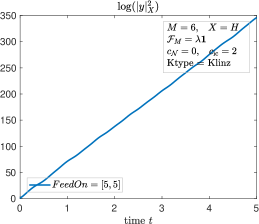
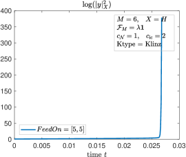
Figure 1. Uncontrolled solutions. Linear and nonlinear systems.

In Figure 2 we see that, with $6$ actuators, the linear feedback is able to stabilize the linear system, for both choices of ${\mathcal{F}}_{M}$. In this example, the choice of ${\mathcal{F}}_{M}=-\nu\Delta+\lambda{\mathbf{1}}$ leads to faster exponential decay rate of the $V$-norm.

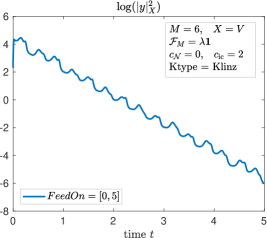
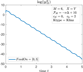
Figure 2. Linear systems and linear feedback.

In Figure 3 we see that the same linear feedback, is not able to stabilize the nonlinear system. This is because the initial condition is too big. Recall that it is known that we can expect such linearization based feedback to be able to stabilize the nonlinear system only if the norm of the initial condition is small enough (local stability).

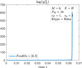
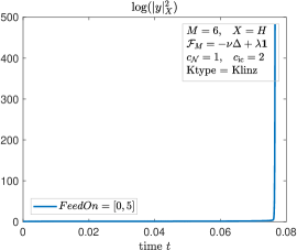
Figure 3. Nonlinear systems and linear feedback.

In Figure 4 we observe that the full nonlinear feedback with $6$ actuators and with ${\mathcal{F}}_{M}=-\nu\Delta+\lambda{\mathbf{1}}$ succeeds to stabilize the solution, while with the choice ${\mathcal{F}}_{M}=\lambda{\mathbf{1}}$ it fails to. The latter choice ${\mathcal{F}}_{M}=\lambda{\mathbf{1}}$ succeeds by taking $7$ actuators.

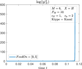
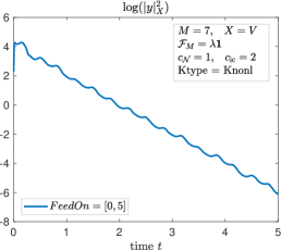
Figure 4. Nonlinear systems and nonlinear feedback.

Figure 5 shows that, for a bigger initial condition, the same nonlinear feedback, with $7$ actuators is not anymore able to stabilize the system for both choices ${\mathcal{F}}_{M}=-\nu\Delta+\lambda{\mathbf{1}}$ and ${\mathcal{F}}_{M}=\lambda{\mathbf{1}}$. Finally, in Figure 6 we observe that by increasing the number $M$ of actuators the nonlinear feedback is again able to stabilize the system. This could give raise to the question on whether by incresing $M$ would also lead to the stability of the linearization based closed-loop system, Figure 7 shows that this is not the case.

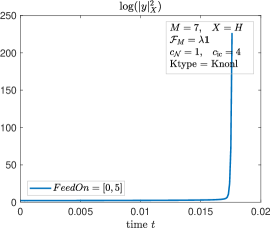
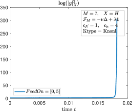
Figure 5. Nonlinear systems and nonlinear feedback. Bigger initial condition.

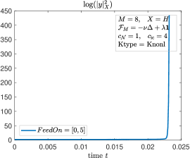
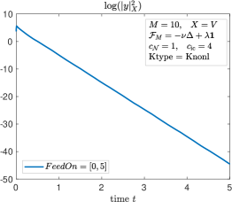
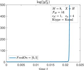
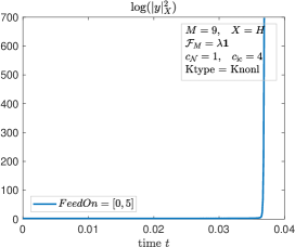
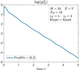
Figure 6. Nonlinear systems and nonlinear feedback. Increasing the number of actuators.

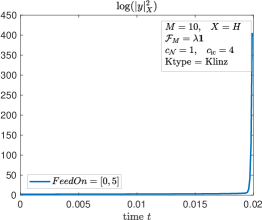
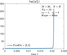
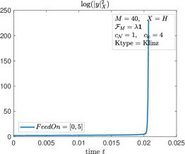
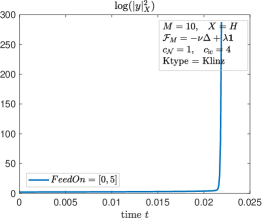
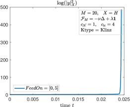
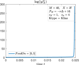
Figure 7. Nonlinear systems and linear feedback. Increasing the number of actuators.

Remark 6.1.

Note that when $q(0)\coloneqq P_{E_{{\mathbb{M}}_{\sigma}}}y(0)=0$, the feedbacks correponding to ${\mathcal{F}}_{{\mathbb{M}}}=\lambda{\mathbf{1}}$ and to ${\mathcal{F}}_{{\mathbb{M}}}=-\nu\Delta+\lambda{\mathbf{1}}$ do coincide, because necessarily the solution $q$ of $\dot{q}={\mathcal{F}}_{{\mathbb{M}}}q$ vanishes in both cases. In particular, the corresponding closed-loop solutions must coincide. This is observed in Figure 8, where we have taken the initial condition $y(0)=\sin(8\pi x)$. Note that, with $M=7$, $E_{{\mathbb{M}}_{\sigma}}=E_{\mathbb{M}}=\mathop{\rm span}\nolimits\{\sin(i\pi x)\mid i\in\{1,2,\dots,7\}\}$ and thus $q(0)=P_{E_{\mathbb{M}}}\sin(8\pi x)=0$.

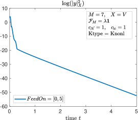
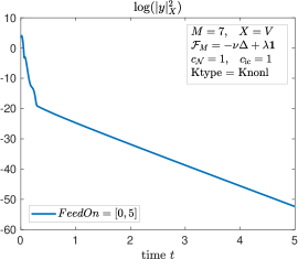
Figure 8. Nonlinear systems and nonlinear feedback. $y(0)=c_{\rm ic}\sin(8\pi x)\in E_{{\mathbb{M}}_{\sigma}}^{\perp}$.

Remark 6.2.

We have taken our $M$ actuators with centers location $c\in[0,1]^{M}$ as in (2.6), which guarantee that the norm $\left|P_{U_{M}}^{E_{\mathbb{M}}}\right|_{{\mathcal{L}}(H)}\leq C_{P}$ remains bounded as $M$ increases, with $C_{P}$ independent of $M$. Since the number $M$ of actuators needed to stabilize the system increase with $C_{P}$, see (4.23), it would be interesting to know the/an optimal location $c=c^{\rm opt}\in[0,1]^{M}$ for the $M$ actuators minimizing $\left|P_{U_{M}}^{E_{\mathbb{M}}}(c)\right|_{{\mathcal{L}}(H)}$. We would like to refer to [37, 38, 28, 47, 39] for works related to finding a/the placement (and/or shape) of actuators, though the functional to be minimized in those works is not $\left|P_{U_{M}}^{E_{\mathbb{M}}}(c)\right|_{{\mathcal{L}}(H)}$.

Appendix

A.1. Proof of Proposition 3.5

We recall the Young inequality [58] as follows: for all $(a,b,\gamma_{0})\in{\mathbb{R}}_{0}^{3}$ and all $s>1$, we have

$$ab=(\gamma_{0}a)(\gamma_{0}^{-1}b)\leq{\textstyle\frac{1}{s}}\gamma_{0}^{s}a^{s}+{\textstyle\frac{s-1}{s}}\gamma_{0}^{-\frac{s}{(s-1)}}b^{\frac{s}{s-1}},$$

Note that $r\coloneqq\frac{s}{s-1}$ satisfies $\frac{1}{s}+\frac{1}{r}=1$. In particular, $ab\leq a^{s}+b^{\frac{s}{s-1}}$. Assumption 3.4 implies that

$$\quad 2\Bigl{(}P_{E_{{\mathbb{M}}_{\sigma}}^{\perp}}^{U_{\#{\mathbb{M}}_{\sigma}}}\left({\mathcal{N}}(t,y_{1})-{\mathcal{N}}(t,y_{2})\right),A(y_{1}-y_{2})\Bigr{)}_{H}$$

$$\leq 2\left|P_{E_{{\mathbb{M}}_{\sigma}}^{\perp}}^{U_{\#{\mathbb{M}}_{\sigma}}}\right|_{{\mathcal{L}}(H)}C_{\mathcal{N}}\textstyle\sum\limits_{j=1}^{n}\left(\left|y_{1}\right|_{V}^{\zeta_{1j}}\left|y_{1}\right|_{{\mathrm{D}}(A)}^{\zeta_{2j}}+\left|y_{2}\right|_{V}^{\zeta_{1j}}\left|y_{2}\right|_{{\mathrm{D}}(A)}^{\zeta_{2j}}\right)\left|y_{1}-y_{2}\right|_{V}^{\delta_{1j}}\left|y_{1}-y_{2}\right|_{{\mathrm{D}}(A)}^{1+\delta_{2j}}$$ (A.1)

and the Young inequality gives us for all $\gamma_{0}>0$, writing for simplicity $\|P\|_{\mathcal{L}}\coloneqq\left|P_{E_{{\mathbb{M}}_{\sigma}}^{\perp}}^{U_{\#{\mathbb{M}}_{\sigma}}}\right|_{{\mathcal{L}}(H)}$,

$$2\Bigl{(}P_{E_{{\mathbb{M}}_{\sigma}}^{\perp}}^{U_{\#{\mathbb{M}}_{\sigma}}}\left({\mathcal{N}}(t,y_{1})-{\mathcal{N}}(t,y_{2})\right),A(y_{1}-y_{2})\Bigr{)}_{H}\leq\textstyle\sum\limits_{j=1}^{n}{\textstyle\frac{(1+\delta_{2j})}{2}}\gamma_{0}^{\frac{2}{1+\delta_{2j}}}\left|y_{1}-y_{2}\right|_{{\mathrm{D}}(A)}^{2}$$

$$\hskip 30.00005pt+\textstyle\sum\limits_{j=1}^{n}{\textstyle\frac{(1-\delta_{2j})}{2}}\left({\textstyle\frac{2C_{\mathcal{N}}}{\gamma_{0}}}\|P\|_{\mathcal{L}}\left|y_{1}-y_{2}\right|_{V}^{\delta_{1j}}\right)^{\frac{2}{1-\delta_{2j}}}\left(\left|y_{1}\right|_{V}^{\zeta_{1j}}\left|y_{1}\right|_{{\mathrm{D}}(A)}^{\zeta_{2j}}+\left|y_{2}\right|_{V}^{\zeta_{1j}}\left|y_{2}\right|_{{\mathrm{D}}(A)}^{\zeta_{2j}}\right)^{\frac{2}{1-\delta_{2j}}}.$$

From [45, Prop. 2.6] we have that $(a_{1}+a_{2})^{s}\leq 2^{\left|s-1\right|}(a_{1}^{s}+a_{2}^{s})$ for $(a_{1},a_{2},s)\in[0,+\infty)$, which implies

$$2\Bigl{(}P_{E_{{\mathbb{M}}_{\sigma}}^{\perp}}^{U_{\#{\mathbb{M}}_{\sigma}}}\left({\mathcal{N}}(t,y_{1})-{\mathcal{N}}(t,y_{2})\right),A(y_{1}-y_{2})\Bigr{)}_{H}\leq\textstyle\sum\limits_{j=1}^{n}{\textstyle\frac{(1+\delta_{2j})}{2}}\gamma_{0}^{\frac{2}{1+\delta_{2j}}}\left|y_{1}-y_{2}\right|_{{\mathrm{D}}(A)}^{2}$$ (A.2)

$$\hskip 10.00002pt+\textstyle\sum\limits_{j=1}^{n}(1-\delta_{2j})2^{\frac{2(1+\delta_{2j})}{1-\delta_{2j}}}\left({\textstyle\frac{C_{\mathcal{N}}}{\gamma_{0}}}\|P\|_{\mathcal{L}}\right)^{\frac{2}{1-\delta_{2j}}}\left(\left|y_{1}\right|_{V}^{\frac{2\zeta_{1j}}{1-\delta_{2j}}}\left|y_{1}\right|_{{\mathrm{D}}(A)}^{\frac{2\zeta_{2j}}{1-\delta_{2j}}}+\left|y_{2}\right|_{V}^{\frac{2\zeta_{1j}}{1-\delta_{2j}}}\left|y_{2}\right|_{{\mathrm{D}}(A)}^{\frac{2\zeta_{2j}}{1-\delta_{2j}}}\right)\left|y_{1}-y_{2}\right|_{V}^{\frac{2\delta_{1j}}{1-\delta_{2j}}}.$$

Observe that if we fix an arbitrary $\widehat{\gamma}_{0}>0$ and set, in (A.2),

$$\gamma_{0}=\gamma_{0j}\coloneqq\left({\textstyle\frac{2}{1+\delta_{2j}}}{\textstyle\frac{\widehat{\gamma}_{0}}{n}}\right)^{\frac{1+\delta_{2j}}{2}}\quad\Longleftrightarrow\quad{\textstyle\frac{\widehat{\gamma}_{0}}{n}}={\textstyle\frac{1+\delta_{2j}}{2}}\gamma_{0j}^{\frac{2}{1+\delta_{2j}}},$$

then, since $\delta_{2j}<1$, we obtain

$$\left({\textstyle\frac{1}{\gamma_{0j}}}\right)^{\frac{2}{1-\delta_{2j}}}=\left({\textstyle\frac{n(1+\delta_{2j})}{2\widehat{\gamma}_{0}}}\right)^{\frac{1+\delta_{2j}}{1-\delta_{2j}}}<\left({\textstyle\frac{n}{\widehat{\gamma}_{0}}}\right)^{\frac{1+\delta_{2j}}{1-\delta_{2j}}}<1+\left({\textstyle\frac{n}{\widehat{\gamma}_{0}}}\right)^{\frac{1+\|\delta_{2}\|}{1-\|\delta_{2}\|}}.$$

with $\|\delta_{2}\|\coloneqq\textstyle\max\limits_{1\leq j\leq n}|\delta_{2j}|$. Hence, we arrive at

$$2\Bigl{(}P_{E_{{\mathbb{M}}_{\sigma}}^{\perp}}^{U_{\#{\mathbb{M}}_{\sigma}}}\left({\mathcal{N}}(t,y_{1})-{\mathcal{N}}(t,y_{2})\right),A(y_{1}-y_{2})\Bigr{)}_{H}\leq\widehat{\gamma}_{0}\left|y_{1}-y_{2}\right|_{{\mathrm{D}}(A)}^{2}$$

$$+\!\left(\!1+\widehat{\gamma}_{0}^{-\frac{1+\|\delta_{2}\|}{1-\|\delta_{2}\|}}\!\right)\!\overline{C}_{\left[n,\|\delta_{2}\|,\frac{1}{1-\|\delta_{2}\|},C_{\mathcal{N}},\|P\|_{\mathcal{L}}\right]}\textstyle\sum\limits_{j=1}^{n}\!\left(\!\left|y_{1}\right|_{V}^{\frac{2\zeta_{1j}}{1-\delta_{2j}}}\!\left|y_{1}\right|_{{\mathrm{D}}(A)}^{\frac{2\zeta_{2j}}{1-\delta_{2j}}}+\left|y_{2}\right|_{V}^{\frac{2\zeta_{1j}}{1-\delta_{2j}}}\!\left|y_{2}\right|_{{\mathrm{D}}(A)}^{\frac{2\zeta_{2j}}{1-\delta_{2j}}}\!\right)\!\left|y_{1}-y_{2}\right|_{V}^{\frac{2\delta_{1j}}{1-\delta_{2j}}}\!.$$

In the particular case $y_{1}=q+Q$ and $y_{2}=q$ with $(q,Q)\in E_{{\mathbb{M}}_{\sigma}}\times E_{{\mathbb{M}}_{\sigma}}^{\perp}$, estimate (A.1) also gives us

$$\quad 2\Bigl{(}P_{E_{{\mathbb{M}}_{\sigma}}^{\perp}}^{U_{\#{\mathbb{M}}_{\sigma}}}\left({\mathcal{N}}(t,q+Q)-{\mathcal{N}}(t,q)\right),AQ\Bigr{)}_{H}$$

$$\leq 2\left\|P\right\|_{{\mathcal{L}}}C_{\mathcal{N}}\textstyle\sum\limits_{j=1}^{n}\left(\left|q+Q\right|_{V}^{\zeta_{1j}}\left|q+Q\right|_{{\mathrm{D}}(A)}^{\zeta_{2j}}+\left|q\right|_{V}^{\zeta_{1j}}\left|q\right|_{{\mathrm{D}}(A)}^{\zeta_{2j}}\right)\left|Q\right|_{V}^{\delta_{1j}}\left|Q\right|_{{\mathrm{D}}(A)}^{1+\delta_{2j}}$$

$$\leq 2(1+2^{\|\zeta-1\|})\left\|P\right\|_{{\mathcal{L}}}C_{\mathcal{N}}\textstyle\sum\limits_{j=1}^{n}\left(\left|q\right|_{V}^{\zeta_{1j}}+\left|Q\right|_{V}^{\zeta_{1j}}\right)\left(\left|q\right|_{{\mathrm{D}}(A)}^{\zeta_{2j}}+\left|Q\right|_{{\mathrm{D}}(A)}^{\zeta_{2j}}\right)\left|Q\right|_{V}^{\delta_{1j}}\left|Q\right|_{{\mathrm{D}}(A)}^{1+\delta_{2j}}$$

$$\leq 2(1+2^{\|\zeta-1\|})\left\|P\right\|_{{\mathcal{L}}}C_{\mathcal{N}}\textstyle\sum\limits_{j=1}^{n}\left(\left|q\right|_{V}^{\zeta_{1j}}+\left|Q\right|_{V}^{\zeta_{1j}}\right)\left|Q\right|_{V}^{\delta_{1j}}\left|Q\right|_{{\mathrm{D}}(A)}^{1+\delta_{2j}+\zeta_{2j}}$$

$$\hskip 30.00005pt+2(1+2^{\|\zeta-1\|})\left\|P\right\|_{{\mathcal{L}}}C_{\mathcal{N}}\textstyle\sum\limits_{j=1}^{n}\left(\left|q\right|_{V}^{\zeta_{1j}}+\left|Q\right|_{V}^{\zeta_{1j}}\right)\left|q\right|_{{\mathrm{D}}(A)}^{\zeta_{2j}}\left|Q\right|_{V}^{\delta_{1j}}\left|Q\right|_{{\mathrm{D}}(A)}^{1+\delta_{2j}}$$

$$\leq 2^{2+\|\zeta-1\|}\left\|P\right\|_{{\mathcal{L}}}C_{\mathcal{N}}\textstyle\sum\limits_{j=1}^{n}\left(\left|q\right|_{V}^{\zeta_{1j}}\left|Q\right|_{V}^{\delta_{1j}}+\left|Q\right|_{V}^{\zeta_{1j}+\delta_{1j}}\right)\left|Q\right|_{{\mathrm{D}}(A)}^{1+\delta_{2j}+\zeta_{2j}}$$

$$\hskip 30.00005pt+2^{2+\|\zeta-1\|}\left\|P\right\|_{{\mathcal{L}}}C_{\mathcal{N}}\textstyle\sum\limits_{j=1}^{n}\left(\left|q\right|_{V}^{\zeta_{1j}}\left|q\right|_{{\mathrm{D}}(A)}^{\zeta_{2j}}\left|Q\right|_{V}^{\delta_{1j}}+\left|q\right|_{{\mathrm{D}}(A)}^{\zeta_{2j}}\left|Q\right|_{V}^{\zeta_{1j}+\delta_{1j}}\right)\left|Q\right|_{{\mathrm{D}}(A)}^{1+\delta_{2j}}$$

with $\|\zeta-1\|\coloneqq\max\{|\zeta_{k,j}-1|\mid 1\leq j\leq n,1\leq k\leq 2\}$. By the Young inequality, with $\gamma_{0}>0$ and $\widetilde{\gamma}_{0}>0$,

$$\quad 2\Bigl{(}P_{E_{{\mathbb{M}}_{\sigma}}^{\perp}}^{U_{\#{\mathbb{M}}_{\sigma}}}\left({\mathcal{N}}(t,q+Q)-{\mathcal{N}}(t,q)\right),AQ\Bigr{)}_{H}\leq\textstyle\sum\limits_{j=1}^{n}\left({\textstyle\frac{1+\delta_{2j}+\zeta_{2j}}{2}}\widetilde{\gamma}_{0}^{{\textstyle\frac{2}{1+\delta_{2j}+\zeta_{2j}}}}+{\textstyle\frac{1+\delta_{2j}}{2}}\gamma_{0}^{{\textstyle\frac{2}{1+\delta_{2j}}}}\right)\left|Q\right|_{{\mathrm{D}}(A)}^{2}$$

$$\hskip 30.00005pt+\textstyle\sum\limits_{j=1}^{n}\left(2^{2+\|\zeta-1\|}\left\|P\right\|_{{\mathcal{L}}}{\textstyle\frac{C_{\mathcal{N}}}{\widetilde{\gamma}_{0}}}\right)^{\frac{2}{1-\delta_{2j}-\zeta_{2j}}}\left(\left|q\right|_{V}^{\zeta_{1j}}\left|Q\right|_{V}^{\delta_{1j}}+\left|Q\right|_{V}^{\zeta_{1j}+\delta_{1j}}\right)^{\frac{2}{1-\delta_{2j}-\zeta_{2j}}}$$

$$\hskip 30.00005pt+\textstyle\sum\limits_{j=1}^{n}\left(2^{2+\|\zeta-1\|}\left\|P\right\|_{{\mathcal{L}}}{\textstyle\frac{C_{\mathcal{N}}}{\gamma_{0}}}\right)^{\frac{2}{1-\delta_{2j}}}\left(\left|q\right|_{V}^{\zeta_{1j}}\left|q\right|_{{\mathrm{D}}(A)}^{\zeta_{2j}}\left|Q\right|_{V}^{\delta_{1j}}+\left|q\right|_{{\mathrm{D}}(A)}^{\zeta_{2j}}\left|Q\right|_{V}^{\zeta_{1j}+\delta_{1j}}\right)^{\frac{2}{1-\delta_{2j}}}$$ (A.3)

Fixing an arbitrary $\widehat{\gamma}_{0}>0$ and setting, in (A.3),

$$\gamma_{0}=\gamma_{0j}\coloneqq\left({\textstyle\frac{2}{1+\delta_{2j}}}{\textstyle\frac{\widehat{\gamma}_{0}}{2n}}\right)^{\frac{1+\delta_{2j}}{2}}\quad\Longleftrightarrow\quad{\textstyle\frac{\widehat{\gamma}_{0}}{2n}}={\textstyle\frac{1+\delta_{2j}}{2}}\gamma_{0j}^{\frac{2}{1+\delta_{2j}}},$$

then, since $\delta_{2j}<1$, we obtain

$$\left({\textstyle\frac{1}{\gamma_{0j}}}\right)^{\frac{2}{1-\delta_{2j}}}=\left({\textstyle\frac{2n(1+\delta_{2j})}{2\widehat{\gamma}_{0}}}\right)^{\frac{1+\delta_{2j}}{1-\delta_{2j}}}<\left({\textstyle\frac{2n}{\widehat{\gamma}_{0}}}\right)^{\frac{1+\delta_{2j}}{1-\delta_{2j}}}<1+\left({\textstyle\frac{2n}{\widehat{\gamma}_{0}}}\right)^{\frac{1+\|\delta_{2}\|}{1-\|\delta_{2}+\zeta_{2}\|}}$$

with $\|\zeta_{2}+\delta_{2}\|\coloneqq\textstyle\max\limits_{1\leq j\leq n}|\delta_{2j}+\zeta_{2j}|$.

Also, with $\widetilde{\gamma}_{0}=\widetilde{\gamma}_{0j}\coloneqq\left({\textstyle\frac{2}{1+\delta_{2j}+\zeta_{2j}}}{\textstyle\frac{\widehat{\gamma}_{0}}{2n}}\right)^{\frac{1+\delta_{2j}+\zeta_{2j}}{2}}\quad\Longleftrightarrow\quad{\textstyle\frac{\widehat{\gamma}_{0}}{2n}}={\textstyle\frac{1+\delta_{2j}+\zeta_{2j}}{2}}\widetilde{\gamma}_{0j}^{\frac{2}{1+\delta_{2j}+\zeta_{2j}}}$, we find $\left({\textstyle\frac{1}{\widetilde{\gamma}_{0j}}}\right)^{\frac{2}{1-\delta_{2j}-\zeta_{2j}}}<1+\left({\textstyle\frac{2n}{\widehat{\gamma}_{0}}}\right)^{\frac{1+\|\delta_{2}\|}{1-\|\zeta_{2}+\delta_{2}\|}}$. Now we show that, from (A.3) we can obtain

$$2\Bigl{(}P_{E_{{\mathbb{M}}_{\sigma}}^{\perp}}^{U_{\#{\mathbb{M}}_{\sigma}}}\left({\mathcal{N}}(t,q+Q)-{\mathcal{N}}(t,q)\right),AQ\Bigr{)}_{H}\leq\widehat{\gamma}_{0}\left|Q\right|_{{\mathrm{D}}(A)}^{2}$$

$$\hskip 20.00003pt+\left(1+\widehat{\gamma}_{0}^{-\frac{1+\|\delta_{2}\|}{1-\|\zeta_{2}+\delta_{2}\|}}\right)\overline{C}\left(1+\left|q\right|_{V}^{2\|\frac{\zeta_{1}+\delta_{1}}{1-\zeta_{2}-\delta_{2}}\|}\right)\left(1+\left|q\right|_{{\mathrm{D}}(A)}^{\|\frac{\zeta_{2}}{1-\delta_{2}}\|}\right)\left(1+\left|Q\right|_{V}^{2\|\frac{\zeta_{1}+\delta_{1}}{1-\zeta_{2}-\delta_{2}}\|-2}\right)\left|Q\right|_{V}^{2}.$$

with the following constants: $\|\frac{\zeta_{1}+\delta_{1}}{1-\zeta_{2}-\delta_{2}}\|\coloneqq\textstyle\max\limits_{1\leq j\leq n}|\frac{\delta_{1j}+\zeta_{1j}}{1-\delta_{2j}-\zeta_{2j}}|$,  $\|\frac{\zeta_{2}}{1-\delta_{2}}\|\coloneqq\textstyle\max\limits_{1\leq j\leq n}|\frac{\zeta_{2j}}{1-\delta_{2j}}|$, and $\overline{C}=\overline{C}_{\left[n,\|\zeta_{1}\|,\|\zeta_{2}\|,\frac{1}{1-\|\delta_{2}\|},\frac{1}{1-\|\delta_{2}+\zeta_{2}\|},C_{\mathcal{N}},\|P\|_{\mathcal{L}}\right]}$. Indeed, we can use the inequalities

$$\left(\left|q\right|_{V}^{\zeta_{1j}}\left|Q\right|_{V}^{\delta_{1j}}+\left|Q\right|_{V}^{\zeta_{1j}+\delta_{1j}}\right)^{\frac{2}{1-\delta_{2j}-\zeta_{2j}}}\leq C_{0}\left(\left|q\right|_{V}^{\frac{2(\zeta_{1j}+\delta_{1j})}{1-\delta_{2j}-\zeta_{2j}}}+\left|Q\right|_{V}^{\frac{2(\zeta_{1j}+\delta_{1j})}{1-\delta_{2j}-\zeta_{2j}}}\right),$$

$$\left(\!\left|q\right|_{V}^{\zeta_{1j}}\!\left|q\right|_{{\mathrm{D}}(A)}^{\zeta_{2j}}\!\left|Q\right|_{V}^{\delta_{1j}}+\left|q\right|_{{\mathrm{D}}(A)}^{\zeta_{2j}}\!\left|Q\right|_{V}^{\zeta_{1j}+\delta_{1j}}\right)^{\frac{2}{1-\delta_{2j}}}\leq C_{1}\!\left(\!\left|q\right|_{V}^{\frac{2\zeta_{1j}}{1-\delta_{2j}}}\left|q\right|_{{\mathrm{D}}(A)}^{\frac{2\zeta_{2j}}{1-\delta_{2j}}}\left|Q\right|_{V}^{\frac{2\delta_{1j}}{1-\delta_{2j}}}+\left|q\right|_{{\mathrm{D}}(A)}^{\frac{2\zeta_{2j}}{1-\delta_{2j}}}\left|Q\right|_{V}^{\frac{2(\zeta_{1j}+\delta_{1j})}{1-\delta_{2j}}}\!\right)$$

$$\hskip 50.00008pt\leq C_{2}\left(1+\left|q\right|_{V}^{\frac{2\zeta_{1j}}{1-\delta_{2j}}}\right)\left|q\right|_{{\mathrm{D}}(A)}^{\frac{2\zeta_{2j}}{1-\delta_{2j}}}\left(\left|Q\right|_{V}^{\frac{2\delta_{1j}}{1-\delta_{2j}}-2}+\left|Q\right|_{V}^{\frac{2(\zeta_{1j}+\delta_{1j})}{1-\delta_{2j}}-2}\right)\left|Q\right|_{V}^{2},$$

where the constants $C_{k}$, $k\in\{1,2,3\}$ are of the form $C_{k}=\overline{C}_{\left[\|\zeta_{1}+\delta_{1}\|,\frac{1}{1-\|\delta_{2}+\zeta_{2}\|},\frac{1}{1-\|\delta_{2}\|}\right]}$. ∎

A.2. Proof of Proposition 4.3

Observe that, since $p\geq 0$, the function $w\mapsto\left|w\right|_{{\mathbb{R}}}^{p}w$ is locally Lipschitz. Therefore, the solutions of (4.18), do exist and are unique, in a small time interval, say for time $t\in[0,\tau)$ with $\tau$ small. When $w_{0}=0$ the solution is the trivial one $w=0$. Note that the equilibria of (4.6), that is, the solutions of $\dot{w}=0$, are given by $\overline{w}_{1}=0$ and $\overline{w}_{2}^{\pm}=\pm\left({\textstyle\frac{\breve{C}_{1}}{\breve{C}_{2}}}\right)^{\frac{1}{p}}$. Furthermore, we observe that $\dot{w}<0$ if $w\in(0,\overline{w}_{2}^{+})$, which implies that the solution issued from $w(s)\in(0,\overline{w}_{2}^{+})$ at time $t=s$, is globally defined, for all time $t\geq s$, is decreasing, and thus remains in $(0,\overline{w}_{2}^{+})$. Note that

$$-\breve{C}_{1}w\leq\dot{w}\leq-\bigl{(}\breve{C}_{1}-\breve{C}_{2}\left|w_{0}\right|_{{\mathbb{R}}}^{p}\bigr{)}w,\quad\mbox{for}\quad w\in(0,\overline{w}_{2}^{+}).$$

Therefore we can conclude that (4.7) holds for $w_{0}\in(0,\overline{w}_{2}^{+})$. Next we consider the case $w_{0}\in(-\overline{w}_{2}^{+},0)$. Denoting the solution issued from $w(s)=w_{s}\in{\mathbb{R}}$, at time $s$, by $w(t)=S(t,s)(w_{s})$, $t\geq s$, we find $S(t,s)(w_{s})=-S(t,s)(-w_{s})$, because with $w^{+}(t)\coloneqq S(t,s)(-w_{s})$, we have

$${\textstyle\frac{\mathrm{d}}{\mathrm{d}t}}(-w^{+})=-\dot{w}^{+}=-\left(-\bigl{(}\breve{C}_{1}-\breve{C}_{2}\left|w^{+}\right|_{{\mathbb{R}}}^{p}\bigr{)}w^{+}\right)=-\bigl{(}\breve{C}_{1}-\breve{C}_{2}\left|-w^{+}\right|_{{\mathbb{R}}}^{p}\bigr{)}(-w^{+}),\qquad-w^{+}(s)=w_{s}.$$

The uniqueness of the solution, implies that $S(t,s)(w_{s})=-w^{+}$. Since $-w_{0}\in(0,\overline{w}_{2}^{+})$, it follows, from above, that $\left|w^{+}\right|_{{\mathbb{R}}}$ satisfies (4.7) and, from $\left|S(t,0)(w_{0})\right|_{{\mathbb{R}}}=\left|w^{+}(t)\right|_{{\mathbb{R}}}$, we obtain that (4.7) holds for $w_{0}\in(-\overline{w}_{2}^{+},0)$. ∎

References

• [1] S. Agmon. Lectures on Elliptic Boundary Value Problems. van Nostrand, 1965. URL: https://bookstore.ams.org/chel-369-h/.
• [2] A. Ambrosetti and G. Prodi. A Primer of Nonlinear Analysis. Cambridge University Press, Cambridge, 1993. URL: https://www.cambridge.org.
• [3] K. Ammari, T. Duyckaerts, and A. Shirikyan. Local feedback stabilisation to a non-stationary solution for a damped non-linear wave equation. Math. Control Relat. Fields, 6(1):1–25, 2016. doi:10.3934/mcrf.2016.6.1.
• [4] S. Aniţa and M. Langlais. Stabilization strategies for some reaction–diffusion systems. Nonlinear Anal. Real World Appl., 10(1):345–357, 2009. doi:10.1016/j.nonrwa.2007.09.003.
• [5] B. Azmi and K. Kunisch. Receding horizon control for the stabilization of the wave equation. Discrete Contin. Dyn. Syst., 38(2):449–484, 2018. doi:10.3934/dcds.2018021.
• [6] M. Badra and T. Takahashi. Stabilization of parabolic nonlinear systems with finite dimensional feedback or dynamical controllers: Application to the Navier–Stokes system. SIAM J. Control Optim., 49(2):420–463, 2011. doi:10.1137/090778146.
• [7] J. M. Ball. Remarks on blow-up and nonexistence theorems for nonlinear evolution equations. Q. J. Math., 28(4):473–486, 1977. doi:10.1093/qmath/28.4.473.
• [8] V. Barbu. Stabilization of Navier–Stokes equations by oblique boundary feedback controllers. SIAM J. Control Optim., 50(4):2288–2307, 2012. doi:10.1137/110837164.
• [9] V. Barbu. Boundary stabilization of equilibrium solutions to parabolic equations. IEEE Trans. Automat. Control, 58(9):2416–2420, 2013. doi:10.1109/TAC.2013.2254013.
• [10] V. Barbu, I. Lasiecka, and R. Triggiani. Abstract settings for tangential boundary stabilization of Navier–Stokes equations by high- and low-gain feedback controllers. Nonlinear Anal., 64:2704–2746, 2006. doi:10.1016/j.na.2005.09.012.
• [11] V. Barbu, S. S. Rodrigues, and A. Shirikyan. Internal exponential stabilization to a nonstationary solution for 3D Navier–Stokes equations. SIAM J. Control Optim., 49(4):1454–1478, 2011. doi:10.1137/100785739.
• [12] V. Barbu and R. Triggiani. Internal stabilization of Navier–Stokes equations with finite-dimensional controllers. Indiana Univ. Math. J., 53(5):1443–1494, 2004. doi:10.1512/iumj.2004.53.2445.
• [13] F. Brauer. Perturbations of nonlinear systems of differential equations. J. Math. Anal. Appl., 14(2):198–206, 1966. doi:10.1016/0022-247X(66)90021-7.
• [14] T. Breiten, K. Kunisch, and S. S. Rodrigues. Feedback stabilization to nonstationary solutions of a class of reaction diffusion equations of FitzHugh–Nagumo type. SIAM J. Control Optim., 55(4):2684–2713, 2017. doi:10.1137/15M1038165.
• [15] L. Chen and A. Jüngel. Analysis of a parabolic cross-diffusion population model without self-diffusion. J. Differential Equations, 224(1):39–59, 2006. doi:10.1016/j.jde.2005.08.002.
• [16] S. Chowdhury and S. Ervedoza. Open loop stabilization of incompressible Navier–Stokes equations in a 2d channel using power series expansion. J. Math. Pures Appl., 2019. doi:/10.1016/j.matpur.2019.01.006.
• [17] J.-M. Coron and H.-M. Nguyen. Null controllability and finite time stabilization for the heat equations with variable coefficients in space in one dimension via backstepping approach. Arch. Rational Mech. Anal., 225(3):993–1023, 2017. doi:10.1007/s00205-017-1119-y.
• [18] F. Demengel and G. Demengel. Functional Spaces for the Theory of Elliptic Partial Differential Equations. Universitext. Springer, 2012. doi:10.1007/978-1-4471-2807-6.
• [19] T. Duyckaerts, X. Zhang, and E. Zuazua. On the optimality of the observability inequalities for parabolic and hyperbolic systems with potentials. Ann. Inst. H. Poincaré Anal. Non Linéaire, 25(1):1–41, 2008. doi:10.1016/j.anihpc.2006.07.005.
• [20] E. Fernández-Cara, M. González-Burgos, S. Guerrero, and J.-P. Puel. Null controllability of the heat equation with boundary Fourier conditions: the linear case. ESAIM Control Optim. Calc. Var., 12(3):442–465, 2006. doi:10.1051/cocv:2006010.
• [21] E. Fernández-Cara, S. Guerrero, O. Yu. Imanuvilov, and J.-P. Puel. Local exact controllability of the Navier–Stokes system. J. Math. Pures Appl., 83(12):1501–1542, 2004. doi:10.1016/j.matpur.2004.02.010.
• [22] J. Fourier. Théorie Analytique de la Chaleur. Firmin Didot, Père et Fils, Paris, 1922.
• [23] A. V. Fursikov and O. Yu. Imanuvilov. Exact controllability of the Navier–Stokes and Boussinesq equations. Russian Math. Surveys, 54(3):565–618, 1999. doi:10.1070/RM1999v054n03ABEH000153.
• [24] A. Halanay, C. M. Murea, and C. A. Safta. Numerical experiment for stabilization of the heat equation by Dirichlet boundary control. Numer. Funct. Anal. Optim., 34(12):1317–1327, 2013. doi:10.1080/01630563.2013.808210.
• [25] P. R. Halmos. Naive Set Theory. Springer, New York, 1974. doi:10.1007/978-1-4757-1645-0.
• [26] O. Yu. Imanuvilov. Remarks on exact controllability for the Navier–Stokes equations. ESAIM Control Optim. Calc. Var., 6:39–72, 2001. doi:10.1051/cocv:2001103.
• [27] D. Kalise and K. Kunisch. Polynomial approximation of high-dimensional Hamilton–Jacobi–Bellman equations and applications to feedback control of semilinear parabolic PDEs. SIAM J. Sci. Comput., 40(2):A629–A652, 2018. doi:10.1137/17M1116635.
• [28] D. Kalise, K. Kunisch, and K. Sturm. Optimal actuator design based on shape calculus. Math. Models Methods Appl. Sci., 28(13):2667–2717, 2018. doi:10.1142/S0218202518500586.
• [29] A. Kröner and S. S. Rodrigues. Internal exponential stabilization to a nonstationary solution for 1D Burgers equations with piecewise constant controls. In Proceedings of the 2015 European Control Conference (ECC), Linz, Austria, pages 2676–2681, July 2015. doi:10.1109/ECC.2015.7330942.
• [30] A. Kröner and S. S. Rodrigues. Remarks on the internal exponential stabilization to a nonstationary solution for 1D Burgers equations. SIAM J. Control Optim., 53(2):1020–1055, 2015. doi:10.1137/140958979.
• [31] K. Kunisch and S. S. Rodrigues. Explicit exponential stabilization of nonautonomous linear parabolic-like systems by a finite number of internal actuators. ESAIM Control Optim. Calc. Var., 2018. doi:10.1051/cocv/2018054.
• [32] K. Kunisch and S. S. Rodrigues. Oblique projection based stabilizing feedback for nonautonomous coupled parabolic-ode systems. RICAM-Report No. 2018-40, 2018. (submitted). URL: https://www.ricam.oeaw.ac.at/publications/ricam-reports/.
• [33] C. Laurent, F. Linares, and L. Rosier. Control and stabilization of the Benjamin–Ono equation in ${L}^{2}(\mathbb{T})$. Arch. Ration. Mech. Anal., 218(3):1531–1575, 2015. doi:10.1007/s00205-015-0887-5.
• [34] H. A. Levine. Some nonexistence and instability theorems for solutions of formally parabolic equations of the form ${P}u_{t}=-{A}u+{\mathcal{F}}(u)$. Arch. Ration. Mech. Anal., 51(5):371–386, 1973. doi:10.1007/BF00263041.
• [35] J.-L. Lions and E. Magenes. Non-Homogeneous Boundary Value Problems and Applications, volume I of Die Grundlehren Math. Wiss. Einzeldarstellungen. Springer-Verlag, 1972. doi:10.1007/978-3-642-65161-8.
• [36] F. Merle and H. Zaag. Optimal estimates for blowup rate and behavior for nonlinear heat equations. Comm. Pure Appl. Math., 51(2):139–196, 1998. doi:10.1002/(SICI)1097-0312(199802)51:2<139::AID-CPA2>3.0.CO;2-C.
• [37] K. Morris. Linear-quadratic optimal actuator location. IEEE Trans. Automat. Control, 56(1):113–124, 2011. doi:10.1109/TAC.2010.2052151.
• [38] K. Morris and S. Yang. A study of optimal actuator placement for control of diffusion. In Proceedings of the 2016 American Control Conference (AAC), Boston, MA, USA, pages 2566–2571, July 2016. doi:10.1109/ACC.2016.7525303.
• [39] A. Münch, P. Pedregal, and F. Periago. Optimal internal stabilization of the linear system of elasticity. Arch. Rational Mech. Anal., 193(1):171–193, 2009. doi:10.1007/s00205-008-0187-4.
• [40] I. Munteanu. Boundary stabilisation to non-stationary solutions for deterministic and stochastic parabolic-type equations. Internat. J. Control, 2017. doi:10.1080/00207179.2017.1407878.
• [41] T. Nagatani, H. Emmerich, and K. Nakanishi. Burgers equation for kinetic clustering in traffic flow. Physica A, 255(1–2), 1998. doi:10.1016/S0378-4371(98)00082-X.
• [42] J. Nagumo, S. Arimoto, and S. Yoshizawa. An active pulse transmission line simulating nerve axon. In Proceedings of the IRE, pages 2061–2070, October 1962. doi:10.1109/JRPROC.1962.288235.
• [43] T. Nambu. Feedback stabilization for distributed parameter systems of parabolic type, II. Arch. Rational Mech. Anal., 79(3), 1882. doi:10.1007/BF00251905.
• [44] E. M. D. Ngom, A. Sène, and D. Y. Le Roux. Global stabilization of the Navier–Stokes equations around an unstable equilibrium state with a boundary feedback controller. Evol. Equ. Control Theory, 4(1):89–106, 2015. doi:10.3934/eect.2015.4.89.
• [45] D. Phan and S. S. Rodrigues. Gevrey regularity for Navier–Stokes equations under Lions boundary conditions. J. Funct. Anal., 272(7):2865–2898, 2017. doi:10.1016/j.jfa.2017.01.014.
• [46] D. Phan and S. S. Rodrigues. Stabilization to trajectories for parabolic equations. Math. Control Signals Syst., 30(2):11, 2018. doi:10.1007/s00498-018-0218-0.
• [47] Y. Privat, E. Trélat, and E. Zuazua. Actuator design for parabolic distributed parameter systems with the moment method. SIAM J. Control Optim., 55(2):1128–1152, 2017. doi:10.1137/16M1058418.
• [48] J.-P. Raymond. Feedback boundary stabilization of the three-dimensional incompressible Navier–Stokes equations. J. Math. Pures Appl., 87(6):627–669, 2007. doi:10.1016/j.matpur.2007.04.002.
• [49] J.-P. Raymond and L. Thevenet. Boundary feedback stabilization of the two-dimensional Navier–Stokes equations with finite-dimensional controllers. Discrete Contin. Dyn. Syst., 27(3):1159–1187, 2010. doi:10.3934/dcds.2010.27.1159.
• [50] S. S. Rodrigues. Feedback boundary stabilization to trajectories for 3D Navier–Stokes equations. Appl. Math. Optim., 2018. doi:10.1007/s00245-017-9474-5.
• [51] S. S. Rodrigues and K. Sturm. On the explicit feedback stabilisation of one-dimensional linear nonautonomous parabolic equations via oblique projections. IMA J. Math. Control Inform., 2018. doi:10.1093/imamci/dny045.
• [52] D. L. Russell. Controllability and stabilizability theory for linear partial differential equations: Recent progress and open questions. SIAM Rev., 20(4):639–739, 1978. doi:10.1137/1020095.
• [53] D. L. Russell and B. Y. Zhang. Exact controllability and stabilizability of the Korteweg–de Vries equation. Trans. Amer. Math. Soc., 348(9):3643–3672, 1996. URL: https://www.jstor.org/stable/2155248.
• [54] R. Temam. Infinite-Dimensional Dynamical Systems in Mechanics and Physics. Number 68 in Appl. Math. Sci. Springer, 2nd edition, 1997. doi:10.1007/978-1-4612-0645-3.
• [55] R. Temam. Navier–Stokes Equations: Theory and Numerical Analysis. AMS Chelsea Publishing, Providence, RI, reprint of the 1984 edition, 2001. Date of access July 12, 2018. URL: https://bookstore.ams.org/chel-343-h.
• [56] M.Y. Wu. A note on stability of linear time-varying systems. IEEE Trans. Automat. Control, 19(2):162, 1974. doi:10.1109/TAC.1974.1100529.
• [57] M. Yamamoto. Carleman estimates for parabolic equations and applications. Inverse Problems, 25(123013), 2009. doi:10.1088/0266-5611/25/12/123013.
• [58] W. H. Young. On classes of summable functions and their Fourier series. Proc. R. Soc. Lond., 87(594):225–229, 1912. doi:10.1098/rspa.1912.0076.