Downlink Transceiver Beamforming and Admission Control for Massive MIMO Cognitive Radio Networks

Shailesh Chaudhari and Danijela Cabric This work has been supported by the National Science Foundation under grant 1149981. Department of Electrical Engineering, University of California, Los Angeles
Email: schaudhari@ucla.edu, danijela@ee.ucla.edu
Abstract

In this paper, an optimization framework is proposed for joint transceiver beamforming and admission control in massive MIMO cognitive radio networks. The objective of the optimization problem is to support maximum number of secondary users in downlink transmission with constraints on the total power allocated to users, the rate achieved at secondary users and the interference at the primary nodes. The proposed framework takes into account the imperfect knowledge of the channels between the secondary and the primary nodes and also mitigates the interference caused by the primary users at secondary receivers. In order to solve the underlying NP-hard problem, we propose a three-step algorithm with two alternative schemes for power allocation, namely: equal power and equal rate. In addition, we provide a solution by reducing the problem to an Integer Linear Program (ILP). The performances of equal rate, equal power, and ILP methods are studied in under different constraints.

Index Terms:
Admission control, interference control, multi-user MIMO.

I Introduction

In cognitive radio (CR) networks, unlicensed secondary users (SUs) co-exist and share the wireless spectrum with licensed primary users (PUs) without causing significant interference to the PUs. There are three paradigms of co-existence of SUs and PUs in a CR network: interweave, overlay and underlay [1]. In this paper, we consider an underlay CR network, where the secondary transmitter is allowed to transmit as long as the interference temperature at primary users (PUs) is below a certain threshold. The interference temperature at the PUs can be controlled by using multiple antennas at the SU transmitter. The multiple-input multiple-output (MIMO) technique allows SU transmitter to employ beamforming to control the interference power transmitted towards the PUs in the network. Further, in multi-user MIMO scenario, by using a large number of antennas at the SU transmitter (massive MIMO), a high number of SU receivers can be served. Various recent research works, such as [2, 3, 4, 5, 6], address the topic of MIMO CR in underlay scenario. However, in [2], a feedback mechanism is required from PU to SU in order to estimate the interference, while [4] requires the perfect knowledge of the channel between the SU transmitter and the PU in order to control the interference. Transmission to multiple SU receivers is not considered in [3]. Papers [5, 6] do not consider interference caused by the PU transmitter at the SU receiver.

In this paper, we consider an underlay cognitive cellular network where a secondary base-station (SU BS) and multiple secondary users (SU UEs) coexist along with PUs. We propose an optimization framework to maximize the number of SU UEs in downlink transmission from the SU BS, which employs a large number of transmit antennas. The constraints of the optimization are as follows: 1) the total power allocated to all SU UEs is limited to $P^{0}$, 2) the minimum rate achieved at any SU UE selected for downlink transmission is $R^{0}$, and 3) the interference power at PUs cannot exceed $I^{0}$. The proposed framework takes into account the imperfect knowledge of the channel between SU BS and PU in line-of-sight (LOS) environment. Further, the optimization framework, unlike [5], and [6], also includes receiver beamforming at SU UEs in order to mitigate the interference caused by PU transmitter.

This paper is organized as follows. The system model is presented in Section II. The error model for the channel estimation is presented in Section III, while the optimization problem is presented in Section IV. The proposed optimization problem is a mixed integer program and a NP-hard problem. We propose a three-step algorithm to solve the transceiver beamforming and admission control problem in Section V. In this section, we also provide a solution to the optimization problem by reducing it to an Integer Linear Program (ILP). The simulation results are presented in Section VI. Finally, Section VII concludes this paper.

II System Model

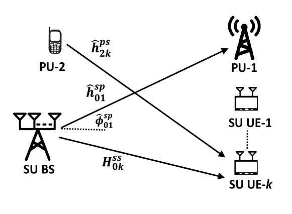
As shown in Fig. 1, we consider a CR network with one SU BS and $K$ SU UEs denoted by SU UE-$k$, $k=1,2,...,K$. The number of antennas at SU BS and SU UEs are denoted by $M_{b}$ and $M_{u}$, respectively, with $M_{b}\gg K$. There are two primary nodes in the network, denoted by PU-1 and PU-2. Both PU-1 and PU-2 have one antenna each. The primary nodes switch the roles from transmitter to receiver and vice-versa.

We consider reciprocal, and line-of-sight (LOS) channels between any two nodes in the network. Let ฮธ0โ€‹ksโ€‹ssubscriptsuperscript๐œƒ๐‘ ๐‘ 0๐‘˜\theta^{ss}_{0k} be the angle at which SU UE-$k$ is located with respect to SU BS and let the corresponding angular sine be ฯ•0โ€‹ksโ€‹s=sinโก(ฮธ0โ€‹ksโ€‹s)subscriptsuperscriptitalic-ฯ•๐‘ ๐‘ 0๐‘˜subscriptsuperscript๐œƒ๐‘ ๐‘ 0๐‘˜\phi^{ss}_{0k}=\sin(\theta^{ss}_{0k}). Then, the MIMO channel between SU BS and SU UE-$k$ is H0โ€‹ksโ€‹s=ฮฒ0โ€‹ksโ€‹sโ€‹aMuโ€‹(ฯ•0โ€‹ksโ€‹s)โ€‹aMbHโ€‹(ฯ•0โ€‹ksโ€‹s)subscriptsuperscript๐ป๐‘ ๐‘ 0๐‘˜subscriptsuperscript๐›ฝ๐‘ ๐‘ 0๐‘˜subscript๐‘Žsubscript๐‘€๐‘ขsubscriptsuperscriptitalic-ฯ•๐‘ ๐‘ 0๐‘˜superscriptsubscript๐‘Žsubscript๐‘€๐‘๐ปsubscriptsuperscriptitalic-ฯ•๐‘ ๐‘ 0๐‘˜H^{ss}_{0k}=\beta^{ss}_{0k}a_{M_{u}}(\phi^{ss}_{0k})a_{M_{b}}^{H}(\phi^{ss}_{0k}), where ฮฒ0โ€‹ksโ€‹s=ฮฑ0โ€‹ksโ€‹sโ€‹ejโ€‹ฯˆ0โ€‹ksโ€‹ssubscriptsuperscript๐›ฝ๐‘ ๐‘ 0๐‘˜subscriptsuperscript๐›ผ๐‘ ๐‘ 0๐‘˜superscript๐‘’๐‘—subscriptsuperscript๐œ“๐‘ ๐‘ 0๐‘˜\beta^{ss}_{0k}=\alpha^{ss}_{0k}e^{j\psi^{ss}_{0k}} and ฮฑ0โ€‹ksโ€‹ssubscriptsuperscript๐›ผ๐‘ ๐‘ 0๐‘˜\alpha^{ss}_{0k}, and ฯˆ0โ€‹ksโ€‹ssubscriptsuperscript๐œ“๐‘ ๐‘ 0๐‘˜\psi^{ss}_{0k} are the channel attenuation and phase, respectively [7]. Let the steering vectors at SU BS and SU UE-$k$ be $a_{M_{b}}(\phi)=[1,e^{j\pi\phi},e^{j\pi 2\phi},...e^{j\pi(M_{b}-1)\phi}]^{H}$ and $a_{M_{u}}(\phi)=[1,e^{j\pi\phi},e^{j\pi 2\phi},...e^{j\pi(M_{u}-1)\phi}]^{H}$, respectively. We assume that the channel attenuation ฮฑ0โ€‹ksโ€‹ssubscriptsuperscript๐›ผ๐‘ ๐‘ 0๐‘˜\alpha^{ss}_{0k} depends on the path-loss, while the phase ฯˆ0โ€‹ksโ€‹ssubscriptsuperscript๐œ“๐‘ ๐‘ 0๐‘˜\psi^{ss}_{0k} is a uniform random variable in $[0,2\pi]$. Similarly, MISO channel between SU BS and PU-2 is h02sโ€‹p=ฮฒ02sโ€‹pโ€‹aMbHโ€‹(ฯ•02sโ€‹p)subscriptsuperscriptโ„Ž๐‘ ๐‘02subscriptsuperscript๐›ฝ๐‘ ๐‘02superscriptsubscript๐‘Žsubscript๐‘€๐‘๐ปsubscriptsuperscriptitalic-ฯ•๐‘ ๐‘02h^{sp}_{02}=\beta^{sp}_{02}a_{M_{b}}^{H}(\phi^{sp}_{02}), where ฮฒ02sโ€‹p=ฮฑ02sโ€‹pโ€‹ejโ€‹ฯˆ02sโ€‹psubscriptsuperscript๐›ฝ๐‘ ๐‘02subscriptsuperscript๐›ผ๐‘ ๐‘02superscript๐‘’๐‘—subscriptsuperscript๐œ“๐‘ ๐‘02\beta^{sp}_{02}=\alpha^{sp}_{02}e^{j\psi^{sp}_{02}}, and SIMO channel between PU-1 and SU UE-$k$ is h1โ€‹kpโ€‹s=ฮฒ1โ€‹kpโ€‹sโ€‹aMuโ€‹(ฯ•1โ€‹kpโ€‹s)subscriptsuperscriptโ„Ž๐‘๐‘ 1๐‘˜subscriptsuperscript๐›ฝ๐‘๐‘ 1๐‘˜subscript๐‘Žsubscript๐‘€๐‘ขsubscriptsuperscriptitalic-ฯ•๐‘๐‘ 1๐‘˜h^{ps}_{1k}=\beta^{ps}_{1k}a_{M_{u}}(\phi^{ps}_{1k}), where ฮฒ1โ€‹kpโ€‹s=ฮฑ1โ€‹kpโ€‹sโ€‹ejโ€‹ฯˆ1โ€‹kpโ€‹ssubscriptsuperscript๐›ฝ๐‘๐‘ 1๐‘˜subscriptsuperscript๐›ผ๐‘๐‘ 1๐‘˜superscript๐‘’๐‘—subscriptsuperscript๐œ“๐‘๐‘ 1๐‘˜\beta^{ps}_{1k}=\alpha^{ps}_{1k}e^{j\psi^{ps}_{1k}}.

Refer to caption
Figure 1: System Model: Massive MIMO Cognitive Radio Network.

III Channel Estimation

We assume that SU BS and SU UEs have the knowledge of the channel H0โ€‹ksโ€‹ssubscriptsuperscript๐ป๐‘ ๐‘ 0๐‘˜H^{ss}_{0k}. However, SU BS does not have a priori knowledge of channels to PUs: h01sโ€‹psubscriptsuperscriptโ„Ž๐‘ ๐‘01h^{sp}_{01} and h02sโ€‹psubscriptsuperscriptโ„Ž๐‘ ๐‘02h^{sp}_{02}. In order to estimate and control the interference power at PU-1 and PU-2, SU BS needs to estimate channel attenuations ฮฑ01sโ€‹psubscriptsuperscript๐›ผ๐‘ ๐‘01\alpha^{sp}_{01} and ฮฑ02sโ€‹psubscriptsuperscript๐›ผ๐‘ ๐‘02\alpha^{sp}_{02} and angular sines ฯ•01sโ€‹psubscriptsuperscriptitalic-ฯ•๐‘ ๐‘01\phi^{sp}_{01} and ฯ•02sโ€‹psubscriptsuperscriptitalic-ฯ•๐‘ ๐‘02\phi^{sp}_{02}.

We assume that the channel attenuation is computed by finding the location of PU-1 using a non-cooperative localization algorithm, such as Weighted Centroid Localization (WCL) [8]. The PU-1 location estimates are then used to obtain the distance d^01sโ€‹psubscriptsuperscript^๐‘‘๐‘ ๐‘01\hat{d}^{sp}_{01} between SU BS and PU-1. The channel attenuation is computed using the path-loss formula: ฮฑ^01sโ€‹p=(d^01sโ€‹p)โˆ’ฮณ/2subscriptsuperscript^๐›ผ๐‘ ๐‘01superscriptsubscriptsuperscript^๐‘‘๐‘ ๐‘01๐›พ2\hat{\alpha}^{sp}_{01}=(\hat{d}^{sp}_{01})^{-\gamma/2}, where $\gamma$ is the path-loss exponent. Similarly, ฮฑ^02sโ€‹psubscriptsuperscript^๐›ผ๐‘ ๐‘02\hat{\alpha}^{sp}_{02} is obtained. The error in the estimation of channel attenuations is modeled as a zero mean Gaussian random variable with variance $\sigma_{\alpha}^{2}$.

Further, in order to estimate the angular sine, ฯ•01sโ€‹psubscriptsuperscriptitalic-ฯ•๐‘ ๐‘01\phi^{sp}_{01}, we assume that SU BS scans the angular space $\phi\in[-1,1]$ at $M_{b}$ equally spaced grid angles when PU-1 is transmitting. The estimated angle ฯ•^01sโ€‹psubscriptsuperscript^italic-ฯ•๐‘ ๐‘01\hat{\phi}^{sp}_{01} is the grid angle at which maximum energy is received. Since the grid angles are separated by $2/M_{b}$, the error in estimation of angular sines is uniformly distributed in range $[-1/M_{b},1/M_{b}]$. Channel attenuation ฮฑ^02sโ€‹psubscriptsuperscript^๐›ผ๐‘ ๐‘02\hat{\alpha}^{sp}_{02} and angular sine ฯ•^02sโ€‹psubscriptsuperscript^italic-ฯ•๐‘ ๐‘02\hat{\phi}^{sp}_{02} are estimated in similar way when PU-2 is transmitting the signal.

IV Optimization Framework

The goal of the proposed optimization framework is to find transmitter and receiver beamforming vectors $v_{k}$ and $u_{k}$, respectively and power allocation $P_{k}$ in order to maximize the number of SU UEs in downlink transmission with given minimum rate requirement, $R^{0}$, while keeping the interference to PUs below a threshold $I^{0}$ with maximum available power constraints $P^{0}$. The optimization problem is presented in (2)-(9).

In (3), the variable skโˆˆ{0,1}subscript๐‘ ๐‘˜01s_{k}\in\{0,1\} indicates whether SU UE-$k$ is selected for transmission (sk=1subscript๐‘ ๐‘˜1s_{k}=1) or not (sk=0subscript๐‘ ๐‘˜0s_{k}=0). All the SU UEs included in downlink transmission have the minimum channel capacity $R^{0}$ as indicated in (4), where $\sigma_{w}^{2}$ is the noise power. The transmitter beamforming constraints in (5) ensure that the beamforming vector $v_{k}$ corresponding to SU UE-$k$ has nulls in the directions of other SU UEs (slโ€‹H0โ€‹lsโ€‹sโ€‹vk=0,kโ‰ lformulae-sequencesubscript๐‘ ๐‘™subscriptsuperscript๐ป๐‘ ๐‘ 0๐‘™subscript๐‘ฃ๐‘˜0๐‘˜๐‘™s_{l}{H}^{ss}_{0l}v_{k}=0,k\neq l). (Note: The constraint โ€–vkโ€–2=sksuperscriptnormsubscript๐‘ฃ๐‘˜2subscript๐‘ ๐‘˜||v_{k}||^{2}=s_{k} ensures that $v_{k}=0$ for sk=0subscript๐‘ ๐‘˜0s_{k}=0). Further, the beamforming vector $v_{k}$ also has nulls in the estimated directions of PU-1 and PU-2 (h^01sโ€‹pโ€‹vk=0,ย โ€‹h^02sโ€‹pโ€‹vk=0formulae-sequencesubscriptsuperscript^โ„Ž๐‘ ๐‘01subscript๐‘ฃ๐‘˜0ย subscriptsuperscript^โ„Ž๐‘ ๐‘02subscript๐‘ฃ๐‘˜0\hat{h}^{sp}_{01}v_{k}=0,\text{ }\hat{h}^{sp}_{02}v_{k}=0). However, due to the angle estimation error ฯ•^01sโ€‹pโˆ’ฯ•01sโ€‹psubscriptsuperscript^italic-ฯ•๐‘ ๐‘01subscriptsuperscriptitalic-ฯ•๐‘ ๐‘01\hat{\phi}^{sp}_{01}-\phi^{sp}_{01}, the constraints in (5) do not place a null at the actual angle ฯ•01sโ€‹psubscriptsuperscriptitalic-ฯ•๐‘ ๐‘01\phi^{sp}_{01}. Therefore, the SU BS needs to estimate the interference power at PU-1 in order to keep it below $I^{0}$. The average interference power at PU-1 is estimated as follows. The power transmitted by SU BS in any arbitrary direction $\phi$ is $\sum_{k=1}^{K}P_{k}v_{k}^{H}a_{M_{b}}({\phi})a_{M_{b}}^{H}({\phi})v_{k}$. Since the estimation error ฯ•01sโ€‹pโˆ’ฯ•^01sโ€‹psubscriptsuperscriptitalic-ฯ•๐‘ ๐‘01subscriptsuperscript^italic-ฯ•๐‘ ๐‘01\phi^{sp}_{01}-\hat{\phi}^{sp}_{01} is uniformly distributed in $[-\frac{1}{M_{b}},\frac{1}{M_{b}}]$, the true value of the angle ฯ•01sโ€‹psubscriptsuperscriptitalic-ฯ•๐‘ ๐‘01\phi^{sp}_{01} lies in the interval [ฯ•^01sโ€‹pโˆ’1/Mb,ฯ•^01sโ€‹p+1/Mb]subscriptsuperscript^italic-ฯ•๐‘ ๐‘011subscript๐‘€๐‘subscriptsuperscript^italic-ฯ•๐‘ ๐‘011subscript๐‘€๐‘[\hat{\phi}^{sp}_{01}-1/M_{b},\hat{\phi}^{sp}_{01}+1/M_{b}] with uniform probability $2/M_{b}$. The average interference power transmitted in the interval [ฯ•^01sโ€‹pโˆ’1/Mb,ฯ•^01sโ€‹p+1/Mb]subscriptsuperscript^italic-ฯ•๐‘ ๐‘011subscript๐‘€๐‘subscriptsuperscript^italic-ฯ•๐‘ ๐‘011subscript๐‘€๐‘[\hat{\phi}^{sp}_{01}-1/M_{b},\hat{\phi}^{sp}_{01}+1/M_{b}] is โˆ‘k=1KPkโ€‹vkHโ€‹Fโ€‹(ฯ•^01sโ€‹p)โ€‹vksuperscriptsubscript๐‘˜1๐พsubscript๐‘ƒ๐‘˜superscriptsubscript๐‘ฃ๐‘˜๐ป๐นsubscriptsuperscript^italic-ฯ•๐‘ ๐‘01subscript๐‘ฃ๐‘˜\sum_{k=1}^{K}P_{k}v_{k}^{H}F(\hat{\phi}^{sp}_{01})v_{k}, where

Fโ€‹(ฯ•^01sโ€‹p)=Mb2โ€‹โˆซฯ•^01sโ€‹pโˆ’1/Mbฯ•^01sโ€‹p+1/MbaMbโ€‹(ฯ•)โ€‹aMbHโ€‹(ฯ•)โ€‹๐‘‘ฯ•.๐นsubscriptsuperscript^italic-ฯ•๐‘ ๐‘01subscript๐‘€๐‘2superscriptsubscriptsubscriptsuperscript^italic-ฯ•๐‘ ๐‘011subscript๐‘€๐‘subscriptsuperscript^italic-ฯ•๐‘ ๐‘011subscript๐‘€๐‘subscript๐‘Žsubscript๐‘€๐‘italic-ฯ•superscriptsubscript๐‘Žsubscript๐‘€๐‘๐ปitalic-ฯ•differential-ditalic-ฯ•F(\hat{\phi}^{sp}_{01})=\frac{M_{b}}{2}\int_{\hat{\phi}^{sp}_{01}-1/M_{b}}^{\hat{\phi}^{sp}_{01}+1/M_{b}}a_{M_{b}}(\phi)a_{M_{b}}^{H}(\phi)d\phi. (1)

Therefore, the estimated interference power at PU-1 is (ฮฑ^01sโ€‹p)2โ€‹โˆ‘k=1KPkโ€‹vkHโ€‹Fโ€‹(ฯ•^01sโ€‹p)โ€‹vksuperscriptsubscriptsuperscript^๐›ผ๐‘ ๐‘012superscriptsubscript๐‘˜1๐พsubscript๐‘ƒ๐‘˜superscriptsubscript๐‘ฃ๐‘˜๐ป๐นsubscriptsuperscript^italic-ฯ•๐‘ ๐‘01subscript๐‘ฃ๐‘˜(\hat{\alpha}^{sp}_{01})^{2}\sum_{k=1}^{K}P_{k}v_{k}^{H}F(\hat{\phi}^{sp}_{01})v_{k}. Similar expression is obtained for the estimated interference power at PU-2. The interference constraints corresponding to PU-1 and PU-2 are included in constraints (6) and (7).

max{uk,vk,Pk,sk}โ€‹โˆ‘k=1Ksk,subscriptsubscript๐‘ข๐‘˜subscript๐‘ฃ๐‘˜subscript๐‘ƒ๐‘˜subscript๐‘ ๐‘˜superscriptsubscript๐‘˜1๐พsubscript๐‘ ๐‘˜\displaystyle\max_{\{u_{k},v_{k},P_{k},s_{k}\}}\sum_{k=1}^{K}s_{k}, (2)
subject to:โ€‹skโˆˆ{0,1},subject to:subscript๐‘ ๐‘˜01\displaystyle\text{subject to:}~{}~{}s_{k}\in\{0,1\}, (3)
Rk=log2โก(1+Pkโ€‹|ukHโ€‹H0โ€‹ksโ€‹sโ€‹vk|2ฯƒw2)โ‰ฅskโ€‹R0,subscript๐‘…๐‘˜subscript21subscript๐‘ƒ๐‘˜superscriptsuperscriptsubscript๐‘ข๐‘˜๐ปsubscriptsuperscript๐ป๐‘ ๐‘ 0๐‘˜subscript๐‘ฃ๐‘˜2superscriptsubscript๐œŽ๐‘ค2subscript๐‘ ๐‘˜superscript๐‘…0\displaystyle R_{k}=\log_{2}\left(1+\frac{P_{k}|u_{k}^{H}H^{ss}_{0k}v_{k}|^{2}}{\sigma_{w}^{2}}\right)\geq s_{k}R^{0}, (4)
h^01sโ€‹pโ€‹vk=0,ย โ€‹h^02sโ€‹pโ€‹vk=0,ย โ€‹โ€–vkโ€–2=sk,ย โ€‹slโ€‹H0โ€‹lsโ€‹sโ€‹vk=0,kโ‰ l,formulae-sequencesubscriptsuperscript^โ„Ž๐‘ ๐‘01subscript๐‘ฃ๐‘˜0formulae-sequenceย subscriptsuperscript^โ„Ž๐‘ ๐‘02subscript๐‘ฃ๐‘˜0formulae-sequenceย superscriptnormsubscript๐‘ฃ๐‘˜2subscript๐‘ ๐‘˜formulae-sequenceย subscript๐‘ ๐‘™subscriptsuperscript๐ป๐‘ ๐‘ 0๐‘™subscript๐‘ฃ๐‘˜0๐‘˜๐‘™\displaystyle\hat{h}^{sp}_{01}v_{k}=0,\text{ }\hat{h}^{sp}_{02}v_{k}=0,\text{ }||v_{k}||^{2}=s_{k},\text{ }s_{l}{H}^{ss}_{0l}v_{k}=0,k\neq l, (5)
(ฮฑ^01sโ€‹p)2โ€‹โˆ‘k=1KPkโ€‹vkHโ€‹Fโ€‹(ฯ•^01sโ€‹p)โ€‹vkโ‰คI0,superscriptsubscriptsuperscript^๐›ผ๐‘ ๐‘012superscriptsubscript๐‘˜1๐พsubscript๐‘ƒ๐‘˜superscriptsubscript๐‘ฃ๐‘˜๐ป๐นsubscriptsuperscript^italic-ฯ•๐‘ ๐‘01subscript๐‘ฃ๐‘˜superscript๐ผ0\displaystyle(\hat{\alpha}^{sp}_{01})^{2}\sum_{k=1}^{K}P_{k}v_{k}^{H}F(\hat{\phi}^{sp}_{01})v_{k}\leq I^{0}, (6)
(ฮฑ^02sโ€‹p)2โ€‹โˆ‘k=1KPkโ€‹vkHโ€‹Fโ€‹(ฯ•^02sโ€‹p)โ€‹vkโ‰คI0,superscriptsubscriptsuperscript^๐›ผ๐‘ ๐‘022superscriptsubscript๐‘˜1๐พsubscript๐‘ƒ๐‘˜superscriptsubscript๐‘ฃ๐‘˜๐ป๐นsubscriptsuperscript^italic-ฯ•๐‘ ๐‘02subscript๐‘ฃ๐‘˜superscript๐ผ0\displaystyle(\hat{\alpha}^{sp}_{02})^{2}\sum_{k=1}^{K}P_{k}v_{k}^{H}F(\hat{\phi}^{sp}_{02})v_{k}\leq I^{0}, (7)
โˆ‘k=1Kskโ€‹Pkโ‰คP0,ย โ€‹Pkโ‰ฅ0,formulae-sequencesuperscriptsubscript๐‘˜1๐พsubscript๐‘ ๐‘˜subscript๐‘ƒ๐‘˜superscript๐‘ƒ0ย subscript๐‘ƒ๐‘˜0\displaystyle\sum_{k=1}^{K}s_{k}P_{k}\leq P^{0},\text{ }P_{k}\geq 0, (8)
ukHโ€‹h^1โ€‹kpโ€‹s=0,ย โ€‹ukHโ€‹h^2โ€‹kpโ€‹s=0,ย โ€‹โ€–ukโ€–2=sk.formulae-sequencesuperscriptsubscript๐‘ข๐‘˜๐ปsubscriptsuperscript^โ„Ž๐‘๐‘ 1๐‘˜0formulae-sequenceย superscriptsubscript๐‘ข๐‘˜๐ปsubscriptsuperscript^โ„Ž๐‘๐‘ 2๐‘˜0ย superscriptnormsubscript๐‘ข๐‘˜2subscript๐‘ ๐‘˜\displaystyle u_{k}^{H}\hat{h}^{ps}_{1k}=0,\text{ }u_{k}^{H}\hat{h}^{ps}_{2k}=0,\text{ }||u_{k}||^{2}=s_{k}. (9)

V Algorithm

The optimization problem described in (2)-(9) is a mixed integer program and therefore, a NP-hard problem. We propose a three-step algorithm to solve the problem. The three steps are: 1) transmitter beamforming 2) receiver beamforming 3) power allocation and interference control. It should be noted that the term ฮ“k=|ukHโ€‹H0โ€‹ksโ€‹sโ€‹vk|2subscriptฮ“๐‘˜superscriptsuperscriptsubscript๐‘ข๐‘˜๐ปsubscriptsuperscript๐ป๐‘ ๐‘ 0๐‘˜subscript๐‘ฃ๐‘˜2\Gamma_{k}=|u_{k}^{H}H^{ss}_{0k}v_{k}|^{2} in (4) represents the equivalent channel strength between SU BS and SU UE-$k$. Since our objective is to serve maximum number of SU UEs with given rate constraints, we maximize the term $\Gamma_{k}$ for $k={1,2,...,K}$ with constraints (5) and (9) in transmitter and receiver beamforming steps, respectively. In step 1 and 2, it is assumed that all the SU UEs are selected for transmission i.e. sk=1,โˆ€ksubscript๐‘ ๐‘˜1for-all๐‘˜s_{k}=1,\forall k. The problem is optimized for variables $P_{k}$ and sksubscript๐‘ ๐‘˜s_{k} in step 3. The algorithmic steps are described below.

V-1 Transmitter Beamforming

The term $\Gamma_{k}$ can be decomposed using H0โ€‹ksโ€‹s=ฮฑ0โ€‹ksโ€‹sโ€‹ejโ€‹ฯˆ0โ€‹ksโ€‹sโ€‹aMuโ€‹(ฯ•0โ€‹ksโ€‹s)โ€‹aMbHโ€‹(ฯ•0โ€‹ksโ€‹s)subscriptsuperscript๐ป๐‘ ๐‘ 0๐‘˜subscriptsuperscript๐›ผ๐‘ ๐‘ 0๐‘˜superscript๐‘’๐‘—subscriptsuperscript๐œ“๐‘ ๐‘ 0๐‘˜subscript๐‘Žsubscript๐‘€๐‘ขsubscriptsuperscriptitalic-ฯ•๐‘ ๐‘ 0๐‘˜superscriptsubscript๐‘Žsubscript๐‘€๐‘๐ปsubscriptsuperscriptitalic-ฯ•๐‘ ๐‘ 0๐‘˜H^{ss}_{0k}=\alpha^{ss}_{0k}e^{j\psi^{ss}_{0k}}a_{M_{u}}(\phi^{ss}_{0k})a_{M_{b}}^{H}(\phi^{ss}_{0k}), as:

ฮ“k=|ukHโ€‹H0โ€‹ksโ€‹sโ€‹vk|2=(ฮฑ0โ€‹ksโ€‹s)2โ€‹|ukHโ€‹aMuโ€‹(ฯ•0โ€‹ksโ€‹s)|2โ€‹|aMbHโ€‹(ฯ•0โ€‹ksโ€‹s)โ€‹vk|2subscriptฮ“๐‘˜superscriptsuperscriptsubscript๐‘ข๐‘˜๐ปsubscriptsuperscript๐ป๐‘ ๐‘ 0๐‘˜subscript๐‘ฃ๐‘˜2superscriptsubscriptsuperscript๐›ผ๐‘ ๐‘ 0๐‘˜2superscriptsuperscriptsubscript๐‘ข๐‘˜๐ปsubscript๐‘Žsubscript๐‘€๐‘ขsubscriptsuperscriptitalic-ฯ•๐‘ ๐‘ 0๐‘˜2superscriptsuperscriptsubscript๐‘Žsubscript๐‘€๐‘๐ปsubscriptsuperscriptitalic-ฯ•๐‘ ๐‘ 0๐‘˜subscript๐‘ฃ๐‘˜2\Gamma_{k}=|u_{k}^{H}H^{ss}_{0k}v_{k}|^{2}=(\alpha^{ss}_{0k})^{2}|u_{k}^{H}a_{M_{u}}({\phi}^{ss}_{0k})|^{2}|a_{M_{b}}^{H}({\phi}^{ss}_{0k})v_{k}|^{2}

In transmitter beamforming, |aMbHโ€‹(ฯ•0โ€‹ksโ€‹s)โ€‹vk|2superscriptsuperscriptsubscript๐‘Žsubscript๐‘€๐‘๐ปsubscriptsuperscriptitalic-ฯ•๐‘ ๐‘ 0๐‘˜subscript๐‘ฃ๐‘˜2|a_{M_{b}}^{H}({\phi}^{ss}_{0k})v_{k}|^{2} is maximized subject to constraints (5). The solution is provided by nullsteering-beamforming algorithm [9], as shown in Algorithm 1.

V-2 Receiver Beamforming

In receiver beamforming, |ukHโ€‹aMuโ€‹(ฯ•0โ€‹ksโ€‹s)|2superscriptsuperscriptsubscript๐‘ข๐‘˜๐ปsubscript๐‘Žsubscript๐‘€๐‘ขsubscriptsuperscriptitalic-ฯ•๐‘ ๐‘ 0๐‘˜2|u_{k}^{H}a_{M_{u}}({\phi}^{ss}_{0k})|^{2} is maximized subject to constraints (9). The solution is provided by nullsteering-beamforming algorithm, as shown in Algorithm 1. In steps 1 and 2, we assume that the channels matrices $H_{0k},k=1,2,...K$ are linearly independent of each other and are also linearly independent of h^01sโ€‹psubscriptsuperscript^โ„Ž๐‘ ๐‘01\hat{h}^{sp}_{01}, and h^02sโ€‹psubscriptsuperscript^โ„Ž๐‘ ๐‘02\hat{h}^{sp}_{02}. This means that aligning the steering vector $v_{k}$ to SU UE-$k$ while placing the nulls towards all the other SU UEs and PUs is not infeasible. Therefore, setting sk=1,โˆ€ksubscript๐‘ ๐‘˜1for-all๐‘˜s_{k}=1,\forall k in oder to maximize ฮ“k=|ukHโ€‹H0โ€‹ksโ€‹sโ€‹vk|2subscriptฮ“๐‘˜superscriptsuperscriptsubscript๐‘ข๐‘˜๐ปsubscriptsuperscript๐ป๐‘ ๐‘ 0๐‘˜subscript๐‘ฃ๐‘˜2\Gamma_{k}=|u_{k}^{H}H^{ss}_{0k}v_{k}|^{2} with constraints (5) and (9), does not result in an infeasible problem. The required condition of channel independence holds in a LOS environment if the angles of SU UEs (ฯ•0โ€‹ksโ€‹ssuperscriptsubscriptitalic-ฯ•0๐‘˜๐‘ ๐‘ \phi_{0k}^{ss}) and PUs (ฯ•^01sโ€‹psubscriptsuperscript^italic-ฯ•๐‘ ๐‘01\hat{\phi}^{sp}_{01} and ฯ•^02sโ€‹psubscriptsuperscript^italic-ฯ•๐‘ ๐‘02\hat{\phi}^{sp}_{02}) are different from each other.

Algorithm 1
1:Receiver Beamforming: $\forall k$, set sk=1subscript๐‘ ๐‘˜1s_{k}=1
2:Maximize |ukHโ€‹aMuโ€‹(ฯ•0โ€‹ksโ€‹s)|2superscriptsuperscriptsubscript๐‘ข๐‘˜๐ปsubscript๐‘Žsubscript๐‘€๐‘ขsubscriptsuperscriptitalic-ฯ•๐‘ ๐‘ 0๐‘˜2|u_{k}^{H}a_{M_{u}}(\phi^{ss}_{0k})|^{2} s. t. constraints (9).
3:Solution: uk=(Iโˆ’PA)โ€‹aMuโ€‹(ฯ•0โ€‹ksโ€‹s)โ€–(Iโˆ’PA)โ€‹aMuโ€‹(ฯ•0โ€‹ksโ€‹s)โ€–subscript๐‘ข๐‘˜๐ผsubscript๐‘ƒ๐ดsubscript๐‘Žsubscript๐‘€๐‘ขsubscriptsuperscriptitalic-ฯ•๐‘ ๐‘ 0๐‘˜norm๐ผsubscript๐‘ƒ๐ดsubscript๐‘Žsubscript๐‘€๐‘ขsubscriptsuperscriptitalic-ฯ•๐‘ ๐‘ 0๐‘˜u_{k}=\frac{(I-P_{A})a_{M_{u}}(\phi^{ss}_{0k})}{||(I-P_{A})a_{M_{u}}(\phi^{ss}_{0k})||}, where $P_{A}=A(A^{H}A)^{-1}A^{H}$ and A=[aMuโ€‹(ฯ•^1โ€‹kpโ€‹s),aMuโ€‹(ฯ•^2โ€‹kpโ€‹s)]๐ดsubscript๐‘Žsubscript๐‘€๐‘ขsubscriptsuperscript^italic-ฯ•๐‘๐‘ 1๐‘˜subscript๐‘Žsubscript๐‘€๐‘ขsubscriptsuperscript^italic-ฯ•๐‘๐‘ 2๐‘˜A=[a_{M_{u}}(\hat{\phi}^{ps}_{1k}),a_{M_{u}}(\hat{\phi}^{ps}_{2k})].
4:Transmitter Beamforming: โˆ€k,l=[1,2โ€‹โ€ฆโ€‹K],lโ‰ kformulae-sequencefor-all๐‘˜๐‘™12โ€ฆ๐พ๐‘™๐‘˜\forall k,l=[1,2...K],l\neq k,
5:Maximize |aMbHโ€‹(ฯ•0โ€‹ksโ€‹s)โ€‹vk|2superscriptsuperscriptsubscript๐‘Žsubscript๐‘€๐‘๐ปsubscriptsuperscriptitalic-ฯ•๐‘ ๐‘ 0๐‘˜subscript๐‘ฃ๐‘˜2|a_{M_{b}}^{H}(\phi^{ss}_{0k})v_{k}|^{2} s. t. constraints (5).
6:Solution: vk=(Iโˆ’PB)โ€‹aMbโ€‹(ฯ•0โ€‹ksโ€‹s)โ€–(Iโˆ’PB)โ€‹aMbโ€‹(ฯ•0โ€‹ksโ€‹s)โ€–,PB=Bโ€‹(BHโ€‹B)โˆ’1โ€‹BHformulae-sequencesubscript๐‘ฃ๐‘˜๐ผsubscript๐‘ƒ๐ตsubscript๐‘Žsubscript๐‘€๐‘subscriptsuperscriptitalic-ฯ•๐‘ ๐‘ 0๐‘˜norm๐ผsubscript๐‘ƒ๐ตsubscript๐‘Žsubscript๐‘€๐‘subscriptsuperscriptitalic-ฯ•๐‘ ๐‘ 0๐‘˜subscript๐‘ƒ๐ต๐ตsuperscriptsuperscript๐ต๐ป๐ต1superscript๐ต๐ปv_{k}=\frac{(I-P_{B})a_{M_{b}}(\phi^{ss}_{0k})}{||(I-P_{B})a_{M_{b}}(\phi^{ss}_{0k})||},P_{B}=B(B^{H}B)^{-1}B^{H} and $B=[a_{M_{b}}(\hat{\phi}^{sp}_{01}),a_{M_{b}}(\hat{\phi}^{sp}_{02})...a_{M_{b}}({\phi}^{ss}_{0l})..]$
7:Power Allocation: (use either scheme 1 or scheme 2)
8:Scheme 1: Equal Power
whileย โˆ‘k=1Kskโ‰ฅ1superscriptsubscript๐‘˜1๐พsubscript๐‘ ๐‘˜1\sum_{k=1}^{K}s_{k}\geq 1ย do
ย ย ย ย ย Pkโ†P0/โˆ‘j=1Ksjโ†subscript๐‘ƒ๐‘˜superscript๐‘ƒ0superscriptsubscript๐‘—1๐พsubscript๐‘ ๐‘—P_{k}\leftarrow P^{0}/\sum_{j=1}^{K}s_{j}
ย ย ย ย ย ifย Rk<skโ€‹R0subscript๐‘…๐‘˜subscript๐‘ ๐‘˜superscript๐‘…0R_{k}<s_{k}R^{0} for any $k$ย then
ย ย ย ย ย ย ย ย ย sj=0,vj=0,uj=0formulae-sequencesubscript๐‘ ๐‘—0formulae-sequencesubscript๐‘ฃ๐‘—0subscript๐‘ข๐‘—0s_{j}=0,v_{j}=0,u_{j}=0, where $j={\text{arg}}\mathop{\min}\limits_{k}R_{k}$.
ย ย ย ย ย endย if
endย while
Scheme 2: Equal Rate
Pkโ†ฯƒw2โ€‹(2R0โˆ’1)|ukHโ€‹H0โ€‹ksโ€‹sโ€‹vk|2โ†subscript๐‘ƒ๐‘˜superscriptsubscript๐œŽ๐‘ค2superscript2superscript๐‘…01superscriptsuperscriptsubscript๐‘ข๐‘˜๐ปsubscriptsuperscript๐ป๐‘ ๐‘ 0๐‘˜subscript๐‘ฃ๐‘˜2P_{k}\leftarrow\frac{\sigma_{w}^{2}(2^{R^{0}}-1)}{|u_{k}^{H}H^{ss}_{0k}v_{k}|^{2}}
whileย โˆ‘k=1Kskโ‰ฅ1superscriptsubscript๐‘˜1๐พsubscript๐‘ ๐‘˜1\sum_{k=1}^{K}s_{k}\geq 1ย do
ย ย ย ย ย ifย โˆ‘k=1Kskโ€‹Pk>P0superscriptsubscript๐‘˜1๐พsubscript๐‘ ๐‘˜subscript๐‘ƒ๐‘˜superscript๐‘ƒ0\sum_{k=1}^{K}s_{k}P_{k}>P^{0}ย then
ย ย ย ย ย ย ย ย ย sj=0,vj=0,uj=0formulae-sequencesubscript๐‘ ๐‘—0formulae-sequencesubscript๐‘ฃ๐‘—0subscript๐‘ข๐‘—0s_{j}=0,v_{j}=0,u_{j}=0, where $j=\text{arg}\mathop{\max}\limits_{k}P_{k}$.
ย ย ย ย ย endย if
endย while
1:Interference Control:
ifย Constraint (6) is not satisfiedย then
sj=0,vj=0,uj=0formulae-sequencesubscript๐‘ ๐‘—0formulae-sequencesubscript๐‘ฃ๐‘—0subscript๐‘ข๐‘—0s_{j}=0,v_{j}=0,u_{j}=0, where j=argโ€‹mink|ฯ•0โ€‹ksโ€‹sโˆ’ฯ•^01sโ€‹p|๐‘—argsubscript๐‘˜subscriptsuperscriptitalic-ฯ•๐‘ ๐‘ 0๐‘˜subscriptsuperscript^italic-ฯ•๐‘ ๐‘01j=\text{arg}\mathop{\min}\limits_{k}|\phi^{ss}_{0k}-\hat{\phi}^{sp}_{01}|.
endย if
ifย Constraint (7) is not satisfiedย then
sj=0,vj=0,uj=0formulae-sequencesubscript๐‘ ๐‘—0formulae-sequencesubscript๐‘ฃ๐‘—0subscript๐‘ข๐‘—0s_{j}=0,v_{j}=0,u_{j}=0, where j=argโ€‹mink|ฯ•0โ€‹ksโ€‹sโˆ’ฯ•^02sโ€‹p|๐‘—argsubscript๐‘˜subscriptsuperscriptitalic-ฯ•๐‘ ๐‘ 0๐‘˜subscriptsuperscript^italic-ฯ•๐‘ ๐‘02j=\text{arg}\mathop{\min}\limits_{k}|\phi^{ss}_{0k}-\hat{\phi}^{sp}_{02}|.
endย if

V-3 Power Allocation and Interference Control

We propose two schemes for power allocation: equal power and equal rate. In addition, we also provide a solution by reducing the problem in an Integer Linear Program (ILP). The transmit- and receive-beamforming vectors, $u_{k}$ and $v_{k}$, obtained in the above steps are treated as constants in this step.

In the equal power scheme, the total available power is distributed equally among the selected SU UEs. Further, if the rate constraints are not satisfied with given power allocation, the SU UE which achieves the minimum rate is removed (by setting sk=0subscript๐‘ ๐‘˜0s_{k}=0) from the downlink transmission. This is because the SU UE achieving the minimum rate despite maximizing $\Gamma_{k}$ in previous steps, has a weak channel $H_{k}$ and will require high power to achieve the rate $R^{0}$. Further, the additional power made available by dropping this SU UE is equally redistributed among the remaining SU UEs and the rate constraints are checked again. The scheme is presented in Algorithm 1.

In the equal rate scheme, the power is allocated such that each SU UE achieves equal rate of $R^{0}$. Further, if the total power constraints ($P^{0}$) are not satisfied, the SU UE that is allocated the maximum power is removed (by setting sk=0subscript๐‘ ๐‘˜0s_{k}=0) from downlink transmission. Again, the reason for dropping this particular SU UE is that it has a weak channel $H_{k}$ which results in high power consumption. Finally, the power constraints are checked again and if they are satisfied, the interference control step is implemented.

In the interference control step, the interference constraints in (6) and (7) corresponding to PU-1 and PU-2 are tested. If the constraint is not satisfied, the SU UE whose angular sine is closest to the angular sine of PU-1 (i.e.|ฯ•0โ€‹ksโ€‹sโˆ’ฯ•^01sโ€‹p|subscriptsuperscriptitalic-ฯ•๐‘ ๐‘ 0๐‘˜subscriptsuperscript^italic-ฯ•๐‘ ๐‘01|\phi^{ss}_{0k}-\hat{\phi}^{sp}_{01}| is minimum) or PU-2, is removed from downlink transmission. This is because the downlink signal transmitted to such SU UE causes the maximum interference at PUs due to proximity in angular domain.

Power Allocation and Interference Control using ILP

In step 3 of the algorithm, by considering $v_{k}$ and $u_{k}$ as constants, the optimization problem (2)-(9) can be reformulated as shown in (10)-(14).

max{Pk,sk}subscriptsubscript๐‘ƒ๐‘˜subscript๐‘ ๐‘˜\displaystyle\max_{\{P_{k},s_{k}\}} โˆ‘k=1Ksk,superscriptsubscript๐‘˜1๐พsubscript๐‘ ๐‘˜\displaystyle\sum_{k=1}^{K}s_{k}, (10)
subject to: skโˆˆ{0,1},subscript๐‘ ๐‘˜01\displaystyle s_{k}\in\{0,1\}, (11)
$\displaystyle R_{k}=\log_{2}\left(1+\frac{P_{k}\Gamma_{k}}{\sigma_{w}^{2}}\right)\geq R^{0},$ (12)
(ฮฑ^0โ€‹jsโ€‹p)2โ€‹โˆ‘k=1Kskโ€‹Pkโ€‹gk,jโ‰คI0,j=1,2,formulae-sequencesuperscriptsubscriptsuperscript^๐›ผ๐‘ ๐‘0๐‘—2superscriptsubscript๐‘˜1๐พsubscript๐‘ ๐‘˜subscript๐‘ƒ๐‘˜subscript๐‘”๐‘˜๐‘—superscript๐ผ0๐‘—12\displaystyle(\hat{\alpha}^{sp}_{0j})^{2}\sum_{k=1}^{K}s_{k}P_{k}g_{k,j}\leq I^{0},j=1,2, (13)
โˆ‘k=1Kskโ€‹Pkโ‰คP0,ย โ€‹Pkโ‰ฅ0formulae-sequencesuperscriptsubscript๐‘˜1๐พsubscript๐‘ ๐‘˜subscript๐‘ƒ๐‘˜superscript๐‘ƒ0ย subscript๐‘ƒ๐‘˜0\displaystyle\sum_{k=1}^{K}s_{k}P_{k}\leq P^{0},\text{ }P_{k}\geq 0 (14)

In the problem, gk,1=vkHโ€‹Fโ€‹(ฯ•^01sโ€‹p)โ€‹vksubscript๐‘”๐‘˜1superscriptsubscript๐‘ฃ๐‘˜๐ป๐นsubscriptsuperscript^italic-ฯ•๐‘ ๐‘01subscript๐‘ฃ๐‘˜g_{k,1}=v_{k}^{H}F(\hat{\phi}^{sp}_{01})v_{k} and gk,2=vkHโ€‹Fโ€‹(ฯ•^02sโ€‹p)โ€‹vksubscript๐‘”๐‘˜2superscriptsubscript๐‘ฃ๐‘˜๐ป๐นsubscriptsuperscript^italic-ฯ•๐‘ ๐‘02subscript๐‘ฃ๐‘˜g_{k,2}=v_{k}^{H}F(\hat{\phi}^{sp}_{02})v_{k}. It should be noted that $g_{k,1}$ and $g_{k,2}$ are non-negative because Fโ€‹(ฯ•^01sโ€‹p)๐นsubscriptsuperscript^italic-ฯ•๐‘ ๐‘01F(\hat{\phi}^{sp}_{01}) and Fโ€‹(ฯ•^02sโ€‹p)๐นsubscriptsuperscript^italic-ฯ•๐‘ ๐‘02F(\hat{\phi}^{sp}_{02}) are positive semi-definite matrices. From (12), it is clear that the minimum feasible power allocation for the $k^{th}$ user in order to achieve the rate $R^{0}$ is $P_{k}=\sigma_{w}^{2}(2^{R^{0}}-1)/\Gamma_{k}$. Further, we note that (ฮฑ^01sโ€‹p)2superscriptsubscriptsuperscript^๐›ผ๐‘ ๐‘012(\hat{\alpha}^{sp}_{01})^{2}, sksubscript๐‘ ๐‘˜s_{k}, $g_{k,1}$, (ฮฑ^02sโ€‹p)2superscriptsubscriptsuperscript^๐›ผ๐‘ ๐‘022(\hat{\alpha}^{sp}_{02})^{2}, and $g_{k,2}$ are non-negative. Therefore, if there exists any feasible power allocation that satisfies constraints (12)-(14) for given skโ€ฒโ€‹ssuperscriptsubscript๐‘ ๐‘˜โ€ฒ๐‘ s_{k}^{\prime}s, then $P_{k}=\sigma_{w}^{2}(2^{R^{0}}-1)/\Gamma_{k}$ is also a feasible power allocation satisfying constraints (12)-(14). Further, since the objective function is independent of $P_{k}$, $P_{k}$โ€™s can be considered as constants with $P_{k}=\sigma_{w}^{2}(2^{R^{0}}-1)/\Gamma_{k}$ and the problem is reduced to an Integer Linear Program (ILP) with binary variables sk,k=1,2,โ€ฆ,Kformulae-sequencesubscript๐‘ ๐‘˜๐‘˜12โ€ฆ๐พs_{k},k={1,2,...,K}, as shown in (15)-(18). This problem can now be solved using standard ILP solvers.

max{sk}subscriptsubscript๐‘ ๐‘˜\displaystyle\max_{\{s_{k}\}} โˆ‘k=1Ksk,superscriptsubscript๐‘˜1๐พsubscript๐‘ ๐‘˜\displaystyle\sum_{k=1}^{K}s_{k}, (15)
subject to: skโˆˆ{0,1},subscript๐‘ ๐‘˜01\displaystyle s_{k}\in\{0,1\}, (16)
(ฮฑ^0โ€‹jsโ€‹p)2โ€‹โˆ‘k=1Kskโ€‹Pkโ€‹gk,jโ‰คI0,j=1,2,formulae-sequencesuperscriptsubscriptsuperscript^๐›ผ๐‘ ๐‘0๐‘—2superscriptsubscript๐‘˜1๐พsubscript๐‘ ๐‘˜subscript๐‘ƒ๐‘˜subscript๐‘”๐‘˜๐‘—superscript๐ผ0๐‘—12\displaystyle(\hat{\alpha}^{sp}_{0j})^{2}\sum_{k=1}^{K}s_{k}P_{k}g_{k,j}\leq I^{0},j=1,2, (17)
โˆ‘k=1Kskโ€‹Pkโ‰คP0,ย โ€‹Pkโ‰ฅ0formulae-sequencesuperscriptsubscript๐‘˜1๐พsubscript๐‘ ๐‘˜subscript๐‘ƒ๐‘˜superscript๐‘ƒ0ย subscript๐‘ƒ๐‘˜0\displaystyle\sum_{k=1}^{K}s_{k}P_{k}\leq P^{0},\text{ }P_{k}\geq 0 (18)

Finally, let us consider a case where a feasible power allocation that satisfies constraints (12)-(14) does not exist. In this case also, we set $P_{k}=\sigma_{w}^{2}(2^{R^{0}}-1)/\Gamma_{k}$ and solve the ILP (15) -(18). The solution of the ILP, in this case, is sk=0,โˆ€ksubscript๐‘ ๐‘˜0for-all๐‘˜s_{k}=0,\forall k.

VI Simulation Results

We consider a CR network spanning over a square-shaped area of $100$m $\times$ $100$m with SU BS located at the origin with x- and y-coordinates $[0,0]$. The location coordinates of PU-1 and PU-2 are $[20,20]$ and $[-30,30]$ respectively. The proposed algorithm is simulated for 1000 iterations, with $K$ SU UEs uniformly distributed in the square-shaped area. The variance of error $(\sigma_{\alpha}^{2})$ in estimation of channel coefficients, $\alpha$, is assumed to be 1% of the true value of $\alpha$.

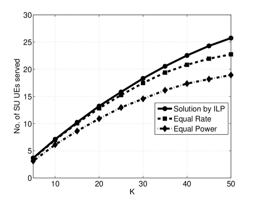
VI-A Impacts of total number of SU UEs and number of antennas

The number of SU UEs selected is plotted against the total number of SU UEs in the network in Fig. 2. It can be observed that the performance of ILP, equal rate, and equal power schemes is comparable if number of users in the network is small ($K<10$). As the number of users in the network increases, the equal power serves fewer users as compared to equal rate and ILP. The equal rate serves more SU UEs than equal rate for the following reason. In both equal rate and equal power schemes, the SU UEs are dropped (by setting sk=0subscript๐‘ ๐‘˜0s_{k}=0) in power allocation and interference control steps. The interference control procedure is the same for both schemes. Therefore, let us consider the power allocation step in the two schemes. In equal rate scheme, the SU UE that is allocated the maximum power is dropped in the power allocation step. Therefore, the cause of interference to PU (SU UE with maximum power) has been removed in power allocation step itself and the interference control step may not be required. On the other hand, in the power allocation step of equal power scheme, the SU UE that achieves the minimum rate is dropped. It should be noted that the SU UE achieving the minimum rate may not cause significant interference to PUs, therefore additional SU UEs are dropped in interference control step in equal power scheme, which results in dropping additional SU UEs from the downlink transmission.

It can be observed that the number of SU UEs increase with higher number of antennas at SU BS in Fig. 3. Increasing $M_{b}$ not only provides more transmission opportunities in angular domain, but also reduces the error in PU angle estimation, which results in higher SU UEs in downlink transmission.
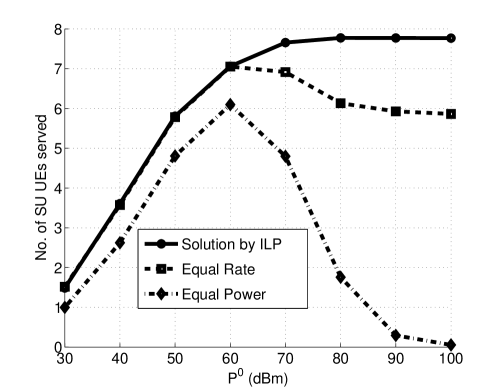
Refer to caption
Figure 2: Number of SU UEs served vs. $K$. Parameters: $M_{b}=128,M_{u}=4$. $I^{0}=0$ dBm, $P^{0}=60$ dBm, $R^{0}=1$ bps/Hz, $\sigma_{w}^{2}=0$ dBm.
Refer to caption
Figure 3: Number of SU UEs served vs. $M_{b}$. Parameters: $K=10,M_{u}=4$. $P^{0}=60$ dBm, $I^{0}=0$ dBm, $\sigma_{w}^{2}=0$ dBm, $R^{0}=1$ bps/Hz.

VI-B Impact of the constraints $P^{0}$, $I^{0}$, $R^{0}$

In order to study the impact of the constraints on the number of SU UEs supported in the downlink, the total number of SU UEs in the network in fixed to $K=10$. The impact of increasing the total power constraint $P^{0}$ is shown in Fig. 4. It is observed that the solution provided by ILP matches with equal rate scheme for $P^{0}\leq 60$ dBm. Equal power scheme served the least number of users among the three schemes. Especially as $P^{0}$ approaches $100$ dBm, the number of users served by equal power scheme reduces to zero. At higher $P^{0}$, the power allocated to each user in equal power scheme is also high. For example, $P_{0}=100$ dBm results in $P_{k}=90$ dBm for each user. This results in a significant interference to the PUs. Therefore, most of the users are dropped from downlink transmission in the interference control step.

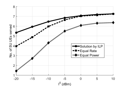
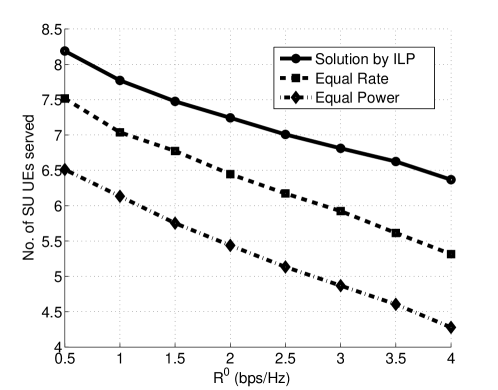
The impact of increasing interference constraint $I^{0}$ is shown in Fig. 5. It can be observed that the performance of equal rate scheme matches that of ILP for $I^{0}\geq 0$ dBm. However, in a stricter interference requirement ($I^{0}=-20$ dBm), the interference control step becomes more important in terms of selecting the SU UEs for downlink transmission. Therefore, the optimum solution provided by ILP is significantly better in terms of serving more user as compared to equal rate scheme. Finally, as shown in Fig. 6, the number of users served in ILP, equal rate, and equal power reduces linearly with increased rate requirement, as expected due to limited available power.

Refer to caption
Figure 4: Number of SU UEs served vs. $P^{0}$. Parameters: $K=10,M_{b}=128,M_{u}=4$. $I^{0}=0$ dBm, $R^{0}=1$ bps/Hz, $\sigma_{w}^{2}=0$ dBm.

VII Conclusion and Future Work

In this paper, we have proposed an optimization framework to maximize the number of SU UEs in downlink transmission from SU BS in a CR network. The optimization problem is constrained by the total power allocated to SU UEs, interference power received at PUs, and minimum rate achieved by the SU UEs selected for the transmission. A three-step algorithm has been proposed to solve the optimization problem using two alternative power allocation schemes, namely equal rate and equal power. In addition, we have also provided a solution by reducing the problem to an ILP. It has been observed that the performance of equal rate and equal power schemes is comparable if the total number of SU UEs is small. For all other scenarios studied, the equal rate scheme serves more SU UEs than equal power. It has been observed that the performance of equal rate matches with the solution provided by ILP under strict power constraints, while the ILP serves more SU UEs than equal rate under strict interference constraints.

In the future work, we would like to develop the algorithm under multipath channels, where the feasibility of the transceiver beamforming depends on the angles of individual paths in the channel at SU BS. Therefore, the channel conditions, and hence the feasibility, should be checked before the beamforming step.

Refer to caption
Figure 5: Number of SU UEs served vs. $I^{0}$. Parameters: $K=10,M_{b}=128,M_{u}=4$. $P^{0}=60$ dBm, $R^{0}=1$ bps/Hz, $\sigma_{w}^{2}=0$ dBm.
Refer to caption
Figure 6: Number of SU UEs served vs. $R^{0}$. Parameters: $K=10,M_{b}=128,M_{u}=4$. $P^{0}=60$ dBm, $I^{0}=0$ dBm, $\sigma_{w}^{2}=0$ dBm.

References

  • [1] E.ย Biglieri, A.ย Goldsmith, L.ย Greenstein, N.ย Mandayam, and H.ย Poor, Principles of Cognitive Radio.ย ย ย Cambridge University Press, 2012.
  • [2] Y.ย Noam and A.ย Goldsmith, โ€œExploiting spatial degrees of freedom in MIMO cognitive radio systems,โ€ in Communications (ICC), 2012 IEEE International Conference on, Jun. 2012, pp. 3499โ€“3504.
  • [3] C.ย Tsinos and K.ย Berberidis, โ€œBlind Opportunistic Interference Alignment in MIMO Cognitive Radio Systems,โ€ vol.ย 3, no.ย 4, pp. 626โ€“639, Dec. 2013.
  • [4] T.ย Xu, L.ย Ma, and G.ย Sternberg, โ€œPractical interference alignment and cancellation for MIMO underlay cognitive radio networks with multiple secondary users,โ€ Dec. 2013.
  • [5] H.ย Du, T.ย Ratnarajah, M.ย Pesavento, and C.ย Papadias, โ€œJoint Transceiver Beamforming in MIMO Cognitive Radio Network Via Second-Order Cone Programming,โ€ IEEE Trans. Signal Process., vol.ย 60, no.ย 2, pp. 781โ€“792, Feb. 2012.
  • [6] H.ย Du and T.ย Ratnarajah, โ€œRobust Utility Maximization and Admission Control for a MIMO Cognitive Radio Network,โ€ IEEE Trans. Veh. Technol., vol.ย 62, no.ย 4, pp. 1707โ€“1718, May 2013.
  • [7] H.ย Q. Ngo, E.ย Larsson, and T.ย Marzetta, โ€œAspects of favorable propagation in Massive MIMO,โ€ in Signal Processing Conference (EUSIPCO), 2014 Proceedings of the 22nd European, Sep. 2014, pp. 76โ€“80.
  • [8] J.ย Wang, P.ย Urriza, Y.ย Han, and D.ย Cabric, โ€œWeighted centroid localization algorithm: Theoretical analysis and distributed implementation,โ€ IEEE Trans. Wireless Commun., vol.ย 10, no.ย 10, pp. 3403โ€“3413, 2011.
  • [9] B.ย Friedlander and B.ย Porat, โ€œPerformance analysis of a null-steering algorithm based on direction-of-arrival estimation,โ€ Acoustics, Speech and Signal Processing, IEEE Transactions on, vol.ย 37, no.ย 4, pp. 461โ€“466, April 1989.