Constraining Cosmology with Big Data Statistics of Cosmological Graphs

Abstract

By utilizing large-scale graph analytic tools implemented in the modern Big Data platform, Apache Spark, we investigate the topological structure of gravitational clustering in five different universes produced by cosmological $N$-body simulations with varying parameters: (1) a WMAP 5-year compatible $\Lambda$CDM cosmology, (2) two different dark energy equation of state variants, and (3) two different cosmic matter density variants. For the Big Data calculations, we use a custom build of stand-alone Spark/Hadoop cluster at Korea Institute for Advanced Study (KIAS) and Dataproc Compute Engine in Google Cloud Platform (GCP) with the sample size ranging from 7 millions to 200 millions. We find that among the many possible graph-topological measures, three simple ones: (1) $\alpha$, (2) $\tau_{\Delta}$, and (3) , can effectively discriminate among the five model universes. Since these graph-topological measures are in direct relation with the usual $n$-points correlation functions of the cosmic density field, graph-topological statistics powered by Big Data computational infrastructure opens a new, intuitive, and computationally efficient window into the dark Universe.

1 Introduction

The evolution of the Universe has imprinted various unique patterns of spatial organization in the cosmic matter distribution. Patterns that have appeared and disappeared across cosmic epochs are accessible to us in the Big Data that is being acquired with astronomical surveys. For understanding the genesis of the Universe and its evolution to the present epoch it is important to extract all the information that is latent in survey data. Subtle diagnostics of spatial organization have the promise to break formidable degeneracies in our picture of the quantum Universe and the nature of gravity.

During the last two decades, studies of the angular anisotropy of the cosmic microwave background (CMB) have provided support for the so-called $\Lambda$CDM cosmological model (e.g., Dunkley et al., 2009; Planck Collaboration et al., 2016a) and have elevated cosmology to an unprecedented level of precision. The baryon acoustic feature, also known as baryon acoustic oscillations (BAO; e.g., Eisenstein et al., 1998, 2005; Shoji et al., 2009; Levi et al., 2013a, b; Ata et al., 2018), has been shown to be an effective “standard ruler” that captures geometric information that is indicative of the universal expansion rate. Numerous galaxy surveys are being performed as well as planned to measure the BAO feature by mapping out the matter distribution of the Universe on large-scales.

The successful measurements of the CMB angular power spectrum and BAO feature show how useful two-point statistics have been for quantifying the geometry of the universe and the evolution of cosmic structure. The more challenging higher-order statistical measurements, such as of the three- and four-point correlation functions (or bi- and tri-spectra of density fluctuations in Fourier space), can provide powerful further constraints that can shed light on a hypothetical non-Gaussianity of primordial quantum fluctuations (e.g., Takahashi, 2014; Planck Collaboration et al., 2016b). The pursuit of primordial non-Gaussianity is just one example how $n$-point statistics provides a unique window into the fundamental physical substrate of the observed Universe.

Along with the successful $n$-point correlation functions, various topological measures have been introduced, such as Betti numbers, Minkowski functionals, and genus statistics (Gott et al., 1987; Eriksen et al., 2004; Park et al., 2013; van de Weygaert et al., 2013; Pranav et al., 2017). To identify specific topological structures such as cosmic filaments and voids, many techniques have been attempted, such as for example wavelets, minimum-spanning trees, Morse theory, watershed transforms, and smoothed Hessians (e.g., Barrow et al., 1985; Sheth et al., 2003; Martinez et al., 2005; Aragón-Calvo et al., 2007; Colberg, 2007; Sousbie et al., 2007; Bond et al., 2010; Cautun et al., 2013). While these topological methods can provide valuable insight, they are generally ad hoc and not (yet) justified within a principled and physically rigorous framework, the kind of framework that justifies the successful $n$-point statistical approaches.

Table 1: Hardware Configurations for the Spark Clusters

	Driver Node		Worker Node
Cluster Name	vCPUs	Memory	vCPUs	Memory	$n$Workers
KIAS Standalone	4	32GB	16	52GB	3
Google Cloud Dataproc	16	104GB	32	208GB	5

As a new way to quantify the elusive topological structure of the Universe, here we apply graph theory (or, network science) to cosmological datasets (Hong & Dey, 2015; Hong et al., 2016, 2019). The basic idea is to associate galaxies with the vertices of a graph and to connect nearby galaxies with graph edges. Then we compute graph-theoretic statistical measures of the cosmic matter distribution as traced by galaxies. We have previously proposed and tested various graph-theoretic topological diagnostic indicators on cosmological datasets, but our attempts to-date were limited to insufficient datasets, ones that were small enough to fit in the memory of workstations. Here, we embrace bleeding-edge technology to overcome this restriction and analyze datasets large enough to extract cosmologically-discriminative statistical indicators.

In this paper, by utilizing the modern Big Data platform, Apache Spark (Zaharia, 2014; Plaszczynski et al., 2018), we investigate the topological structure of five different universes, all generated with cosmological $N$-body simulations with various input parameters but seeded with same realization of a Gaussian random field. The galaxy sample size extracted from the simulations ranged from 7 million to 200 million galaxies. To calculate graph statistics of these Big Data samples, we built our own stand-alone Spark/Hadoop cluster at the Korea Institute for Advanced Study (KIAS) and also used the commercial cloud cluster, the Cloud Dataproc service within the Google Cloud Platform (GCP), for some of the calculations that required more computation resources than what the KIAS stand-alone cluster could provide. We summarize the hardware specifications of these clusters in Table 1.

This paper is organized as follows. In Section 2, we describe our $N$-body simulations, which we name Multiverse, and how we generated graphs from the simulation data. In Section 3, we present a mathematical formulation of the graph statistical methods and in Section 4 we apply the methods to our datasets and propose a diagnostic scheme that discriminates between the five different universes. Finally, in Section 5, we summarize our results and list our conclusions. We interchangeably use the terminology of graph theory and network science, such as vertex vs. node, edge vs. link, and graph vs. network.

2 DATA

2.1 Multiverse Simulations

The Multiverse Simulations are a set of cosmological pure $N$-body simulations designed to study the effect of cosmological parameters on the formation of large-scale structures (LSS) in various universe models as traced by galaxies (Kim et al. in prep.). The fiducial simulation is based on the concordance $\rm\Lambda$CDM model with $H_{0}=100\,h\,\text{km}\,\text{s}^{-1}\,\text{Mpc}^{-1}$ where $h=0.72$, $\Omega_{\rm m}=0.26$, $\Omega_{\Lambda}=0.74$, $\Omega_{\rm b}=0.044$, $w=-1$ and $b_{8}=1.2$ (hereafter, we refer to this fiducial universe as “standard universe” denoted by STD). Here, $w$ is the pressure-to-energy density ratio that parametrizes the equation of state of the dark energy. The shape of linear power spectrum was obtained from the CAMB code and its power spectral amplitude is tuned to make the density fluctuations satisfy the relation $\sigma_{8}\equiv 1/b_{8}$. Here, $\sigma_{8}$ is the standard deviation of the density field when smoothed with a top-hat spherical kernel with radius $R_{\rm tophat}=8~{}h^{-1}\,\text{Mpc}$ at $z=0$. We placed the simulation particles at grid points as pre-initial conditions and perturbed them using the second-order linear perturbation method. The gravitational evolution of particles was performed with the GOTPM code (Dubinski et al., 2004) that solves the Poisson equation with the Fast-Fourier-Transforms (FFT) and corrects the short-range force with the Barnes-Hut tree method.

For the non-standard-$\Lambda$CDM simulations, we adopt four variant models different from our fiducial $\Lambda$CDM in a single parameter:

• DM1: $\Omega_{\rm m}=0.31$,

• DM2: $\Omega_{\rm m}=0.21$,

• DE1: $w=-0.5$,

• DE2: $w=-1.5$.

The same random number sequence is applied to generating initial conditions, which may eliminate the cosmic variances between simulated models. Therefore, it would be possible to study the pure cosmological effects on structure and galaxy formation by directly comparing the distributions of cosmic objects. The number of particles in each simulation is $N_{\rm p}=2048^{3}$. We integrate the gravitational evolution of the models starting redshift of $z_{\rm init}=99$ to the final epoch $z=0$ with 1980 steps. The simulation box size is $L_{\rm box}=1024~{}h^{-1}\,\text{Mpc}$ in the comoving scale.

Figure 1: Simulated matter power spectra of the Multiverse Simulations at $z_{\rm init}=99$ and $z=0$. The dotted lines are the linear power spectrum of the standard universe, STD.

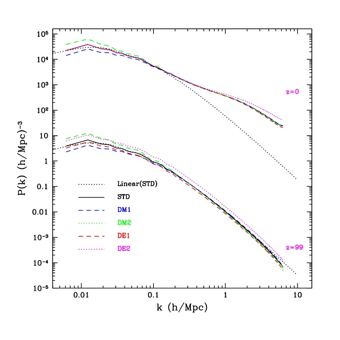
Figure 1 shows the simulated mass power spectra (colored solid lines) of the Multiverse simulations compared to the linear expectation of the $\rm\Lambda$CDM model (dotted lines). At $z=0$, the small-scale power spectrum of DE2 has a relatively higher amplitude than that of the other simulations. This difference is mainly due to the higher power amplitude of DE2 at the starting redshift that makes the small-scale perturbation enter the nonlinear regime earlier.

Figure 2: The two-point correlation functions for equal mass cut sample (left), $M_{\rm cut}=5\times 10^{11}h^{-1}$ M_⊙, and equal abundance sample (right), $N_{h}=7,086,717$. The grey error bars represent the bootstrap resampling errors for STD. The other Multiverses show similar bootstrap errors, skipped in the panels due to the redundancy.

For generating halo catalogs, we extract virialized halos with the minimum mass of $M_{\rm min}=2.7\times 10^{11}(\Omega_{\rm m}/0.26)~{}h^{-1}{\rm M_{\odot}}$, which corresponds to a minimum of 30 particles. We have used the standard Friends-of-Friends method with linking length $l_{\rm FoF}=0.2\times l_{\rm mean}$ where $l_{\rm mean}$ is the average distance between particles.

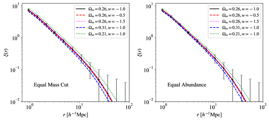
From the halo catalogs, we select two kinds of samples with (1) equal mass cut, $M_{\rm cut}=5\times 10^{11}h^{-1}$ M_⊙, and (2) equal abundance cut, $N_{\rm h}=7,086,717$, corresponding to a comoving density of $n_{\rm h}=6.6\times 10^{-3}\big{[}h^{-1}$Mpc$\big{]}^{-3}$, as summarized in Table 2. Figure 2 shows the two-point correlation function for each halo selection criterion. The grey error bars represent the conventional bootstrap resampling errors for STD.

For graph measurements, any reshuffling by resampling can affect the graph connectivity. Therefore, instead of resampling to measure cosmic variances of graph statistics, we use a halo catalog from Horizon Run 4 (Kim et al., 2015, hereafter, STD-HR), which has the same cosmological parameters as STD, but a much larger volume of ($3,150$ $h^{-1}$ Mpc)³. Hence, at least for STD, we can measure the comic variance of graph statistics directly by subsampling the STD-HR catalog. Thanks to Apache Spark we can easily handle this Big Data catalog that is composed of 206 millions halos.

Table 2: Sample Selections

Multiverses		Equal Mass Cut Sample		Equal Abundance Sample
Name	Cosmological Parameters	$N_{h}$	$M_{\rm cut}$($h^{-1}$ M⊙)	$N_{h}$	$M_{min}$($h^{-1}$M⊙)
STD	$\Omega_{\rm m}=0.26,w=-1.0$	7,086,717	$5.00\times 10^{11}$	7,086,717	$5.05\times 10^{11}$
DE1	$\Omega_{\rm m}=0.26,w=-0.5$	7,806,135	$5.00\times 10^{11}$	7,086,717	$5.59\times 10^{11}$
DE2	$\Omega_{\rm m}=0.26,w=-1.5$	6,886,870	$5.00\times 10^{11}$	7,086,717	$4.87\times 10^{11}$
DM1	$\Omega_{\rm m}=0.31,w=-1.0$	8,595,923	$5.00\times 10^{11}$	7,086,717	$6.24\times 10^{11}$
DM2	$\Omega_{\rm m}=0.21,w=-1.0$	5,579,491	$5.00\times 10^{11}$	7,086,717	$3.86\times 10^{11}$
STD-HR	Horizon Run	206,140,716	$5.00\times 10^{11}$	206,140,716	$5.05\times 10^{11}$

2.2 Generating Halo Networks

To build a network from each halo distribution, we use the conventional FoF recipe (Huchra & Geller, 1982; Hong & Dey, 2015; Hong et al., 2016, 2019). For a given linking length $l$, the adjacency matrix of the FoF recipe can be written as,

$$A_{ij}=\left\{\begin{array}[]{ll}1&\textrm{ if }r_{ij}\leq l,\\ 0&\textrm{ otherwise, }\end{array}\right.$$ (1)

where $r_{ij}$ is the distance between the two vertices (i.e., galaxies), $i$ and $j$. This binary matrix is essential in graph analysis as it quantifies network connectivity. Interested readers can consult Albert & Barabási (2002), Newman (2003), Dorogovtsev et al. (2008), and Barthélemy (2011) for further information.

3 Statistics of Graph Configurations

In this section, we present basic graph quantities and their definitions used in network science (Dall & Christensen, 2002; Barthélemy, 2011). Then, we show how each graph quantity is related to $n$-point correlation functions. The details of mathematical derivations can be found in a separate paper (Jeong et al. 2019, in prep.).

3.1 Basic Quantities

First, we define two basic quantities,

$$\alpha \equiv \frac{2K}{N},$$ (2)

$$p \equiv \frac{2K}{N(N-1)},$$ (3)

where $N$ is the total number of vertices and $K$ the total number of edges. We define $degree$ as the number of neighbors for each vertex. Then, $\alpha$ means the average of all degrees for the network; generally referred to as average degree in network science. $p$ is the fraction of real connected edges out of the total pair-wise combinations, $N(N-1)/2$; referred to as edge density. Finally, $\alpha$ and $p$ satisfy this trivial equality,

$$\alpha = p(N-1).$$ (4)

3.1.1 Ensemble Average and Random Poisson Graph

If we can define an ensemble of graphs, we can derive many graph statistics from probability distribution functions based on ensemble averages. Let us assume that we have a graph ensemble, denoted by $G_{\alpha,p}$ for given $\alpha$ and $p$. The average degree, $\alpha$, now can be written using a degree distribution, $p_{k}$, as

$$\alpha = \sum_{k=0}^{\infty}k\times p_{k},$$ (5)

where $k$ is a degree and $p_{k}$ a probability density for given $k$ with the normalization of $\sum_{k=0}^{\infty}p_{k}=1$. If we randomly connect two vertices using the probability, $p$, in Equation 3 (i.e., generating random graphs), the degree distribution of this ensemble is Poissonian,

$$p_{k} \simeq \frac{\alpha^{k}e^{-\alpha}}{k!},$$ (6)

in the limit of large $N$. To discern these random graphs from random geometric graphs in the following section, we refer to this kind as Random Poisson Graph (RPG).

3.1.2 Geometric Graphs and Correlation Functions

Now, we consider a graph embedded in a metric space; specifically, in this paper, $d$dimensional Euclidean space. Since RPG described in the previous section has no geometric restriction, it can be described by only two parameters, $N$ and $K$; or, corresponding $\alpha$ and $p$.

For geometric graphs, we have additional quantities: (1) spatial dimension, $d$, (2) total system volume, $V$, and (3) linking length for connections, $l$, along with $N$ and $K$. Based on these parameters, determining geometric graphs, we define three basic quantities, the spatial number density, $\bar{n}$, excluded volume, $V_{l}$, and fraction of excluded volume, $q$,

$$\bar{n} \equiv \frac{N}{V},$$ (7)

$$V_{l} \equiv \frac{\pi^{d/2}l^{d}}{\Gamma\big{(}\frac{d+2}{2}\big{)}},$$ (8)

$$q \equiv \frac{V_{l}}{V},$$ (9)

where $\Gamma(x)$ is the gamma function. Then, for $d=3$, $\alpha$ and $p$ can be derived as,

$$\alpha = \bar{n}\int_{V_{l}}d^{3}r[1+\xi(r)],$$ (10)

$$p \simeq \frac{1}{V}\int_{V_{l}}d^{3}r[1+\xi(r)],$$ (11)

using 2-point correlation function, $\xi(r)$ (Jeong et al., in prep.).

Unlike the simple derivations of $\alpha$ and $p$, the degree distribution, $p_{k}$, is inevitably complex determined by all orders of correlation functions,

$$p_{k} \sim \mathcal{F}(\{C_{k=1,2,\cdots}\}),$$ (12)

where $C_{k}$ represents $k$-point correlation function. since random geometric graphs (RGGs) have null correlation functions, Equation 10, 11, and 12 for RGGs are as simple as,

$$\alpha = \bar{n}V_{l},$$ (13)

$$p \simeq q,$$ (14)

$$p_{k} \simeq \frac{\alpha^{k}e^{-\alpha}}{k!}.$$ (15)

Hence, any deviations of cosmological networks from these RGGs are caused by the non-zero correlation functions of cosmic datasets.

Figure 3: The percolation threshold, $\alpha_{c}$, and giant component fraction, $S$, for RPGs. The left panel demonstrates which $\alpha$ results in the non-zero solution of giant component fraction, $S$. The right panel summarizes the analytic solutions in the plot of $S(\alpha)$ vs. $\alpha$. The grey dashed line represents the mean values of simulated results for RPGs with $N=10^{3}$ vertices, and the grey shaded area the $\pm 1\sigma$ variations. In the Big Data regime, i.e., $N\to\infty$, the simulated giant component fractions converge to the theoretical line.

3.2 Giant Component and Percolation Threshold

The giant component is the largest connected subgraph in a network. The fraction, $S$, of vertices belonging to the giant component can be written using a generating function, $G_{0}(x)$, as

$$S = 1-G_{0}(u),$$ (16)

$$G_{0}(x) = \sum_{k=0}^{\infty}p_{k}x^{k},$$ (17)

where $u$ is the probability of a vertex, not belonging to the giant component, which satisfies a self-consistent equation,

$$u = G_{1}(u),$$ (18)

where $G_{1}(x)=G^{\prime}_{0}(x)/G^{\prime}_{0}(1)$ (Dall & Christensen, 2002; Barthélemy, 2011). For the Poissonian degree distribution of RPGs, we can solve Equation 16 as

$$S = 1-e^{-\alpha S},$$ (19)

or,

$$\alpha S = -\ln(1-S).$$ (20)

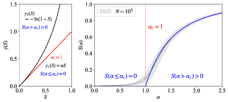
Figure 3 shows the solution of Equation 20. The left panel shows that $S=0$ is the only non-negative solution for $\alpha\leq 1$. For $\alpha>1$, $S$ increases monotonically to the asymptotic value $S=1$. The right panel summarizes the solution of the left panel, showing $S(\alpha)$ vs. $\alpha$. The trainsition of $S(\alpha)$ happens at the percolation threshold for RPGs, $\alpha_{c}=1$.

RGGs also have Poissonian degree distributions. The difference from RPGs is that the connections are determined by a connecting hyper-sphere, depending on spatial dimensionality, while RPGs only depending on the single parameter, $p$. Dall & Christensen (2002) reported the percolation thresholds of RGGs for various dimensions, $d$, as $\alpha_{c}(d=2)=4.52$, $\alpha_{c}(d=3)=2.74$, and $\alpha_{c}(d=\infty)\simeq 1$ .

3.3 Transitivity and 3-point Correlation Function

Figure 4: The graph schematic for describing the meaning of transitivity, $\tau_{\Delta}$. The two connected sides, $r_{1}$ and $r_{2}$, form a connected triple; i.e., a “$\vee$” configuration. If the other side, $r_{12}$, is also connected, then we refer to this triangular triple as a closed triple. Transitivity is a ratio of closed triples to connected triples. This value can be written using $2-$ and $3-$point correlation functions as Equation 22.

Figure 5: The graph schematic for transitivity, $\tau_{\Delta}$, and average local clustering coefficient, $\overline{C}$. The number on each node circle represents the local clustering coefficient, $C_{i}$, as defined in Equation 25 and $k$ the number of neighbors (i.e., degree). The average of local clustering coefficients, $\overline{C}$, is $\frac{7}{12}$ (or, $\frac{7}{9}$ when excluding the node with $k=1$ for the average, of which denominator is zero), different from the transitivity, $\frac{3}{5}$.

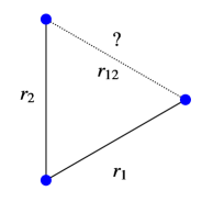
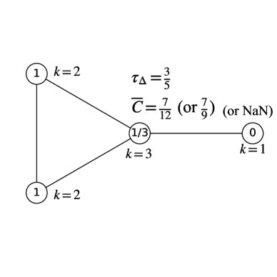
Figure 4 shows a triple of which two sides, $r_{1}$ and $r_{2}$, are connected. This configuration is referred to as a connected triple; if the other side, $r_{12}$, is also connected, a closed triple. The transitivity, $\tau_{\Delta}$, is a triangular density defined using these triple configurations as,

$$\tau_{\Delta} \equiv \frac{\textrm{number of closed triples}}{\textrm{number of connected triples}}.$$ (21)

For cosmological networks embedded in 3d comoving volume, we can rewrite this equation using correlation functions as,

$$\tau_{\Delta} = \frac{\displaystyle\int_{V_{l}}d^{3}r_{1}\int_{V_{l}}d^{3}r_{2}~{}p_{3}(\bm{r_{1}},\bm{r_{2}})\Theta(l-r_{12})}{\displaystyle\int_{V_{l}}d^{3}r_{1}\int_{V_{l}}d^{3}r_{2}~{}p_{3}(\bm{r_{1}},\bm{r_{2}})},$$ (22)

$$p_{3}(\bm{r_{1}},\bm{r_{2}}) \equiv \bar{n}^{3}\big{[}1+\xi(r_{1})+\xi(r_{2})+\xi(r_{12})+\zeta(r_{1},r_{2},r_{12})\big{]},$$ (23)

where $\xi(x)$ is 2-point correlation function, $\zeta(x,y,z)$ 3-point correlation function, and $\Theta(x)$ the Heaviside step function (Jeong et al. in prep). For RGGs, since their correlation functions vanish, we can derive the transitivities as,

$$\tau_{\Delta} = \frac{3}{\sqrt{\pi}}\frac{\Gamma(\frac{d+2}{2})}{\Gamma(\frac{d+1}{2})}\int_{0}^{\pi/3}\sin^{d}\theta d\theta,$$ (24)

for arbitrary $d$-dimensions (Dall & Christensen, 2002).

We can define a transitivity-like quantity for each vertex. When assuming that a vertex, $i$, has $k_{i}$ neighbors and the number of triangles centered on this vertex is $\Delta_{i}$, we can write down a transitivity-like quantity for this vertex, $C_{i}$, as,

$$C_{i} \equiv \frac{2\Delta_{i}}{k_{i}(k_{i}-1)},$$ (25)

where $k_{i}(k_{i}-1)/2$ is the total number of connected triples (or, “$\vee$” configurations) and $\Delta_{i}$ the total number of closed triples on this vertex. This vertex-wise transitivity is referred to as local clustering coefficient (LCC). Then, the average LCC, $\overline{C}$, can be written as,

$$\overline{C} = \frac{1}{N}\sum_{i=1}^{N}C_{i}.$$ (26)

Due to this averaging process, $\overline{C}$ is biased to the major population of vertices. For example, if a galaxy catalog is dominated by field galaxies, the triangular configurations formed by dense group galaxies are underrepresented in this statistic, while transitivity is an unbiased network-wise (not, vertex-wise) measurement. Figure 5 shows a schema demonstrating the definitions of $\tau_{\Delta}$ and $\overline{C}$.

4 Results

4.1 Statistics of Graph Configurations

Figure 6 and 7 show graph statistics of the five Multiverses for the two sample selections (1) equal mass cut, $M_{\rm cut}=5\times 10^{11}h^{-1}$ M_⊙, and (2) equal abundance cut, $N_{h}=7,086,717$ as summarized in Table 2. Each panel shows the giant component fraction ($S_{1}$; top-left), the second giant component fraction ($S_{2}$; top-right), the transitivity ($\tau_{\Delta}$; middle-left), the average local clustering coefficient ($\overline{C}$; middle-right), the number densities for the connected subcomponents with $s=2,3,4$ ($n_{s=2,3,4}$; bottom-left), and the cumulative number density of all subcomponents with $s\geq 5$ ($n_{s\geq 5}$; bottom-right).

4.1.1 Equal Mass Cut Sample: $M_{\rm cut}=5.0\times 10^{11}h^{-1}$ M_⊙

Figure 6: The graph statistics vs. the linking lengths for the Multiverse Simulations: Giant Component Fraction ($S_{1}$, top-left), Second Giant Component Fraction ($S_{2}$, top-right), Transitivity ($\tau_{\Delta}$, middle-left), Average Local Clustering Coefficient ($\overline{C}$, middle-right), number densities for the connected subcomponents with $s=2,3,4$ ($n_{s=2}$, $n_{s=3}$, $n_{s=4}$, bottom-left), and cumulative number density of all subcomponents with $s\geq 5$ ($n_{s\geq 5}$, bottom-right). As summarized in Table 1, we have two kinds of halo samples, using (1) equal mass cut, $M_{h}\geq 5\times 10^{11}h^{-1}$M_⊙, and (2) eqaul abundance cut, $N_{h}=7,086,717$. This figure is for the equal mass cut sample.

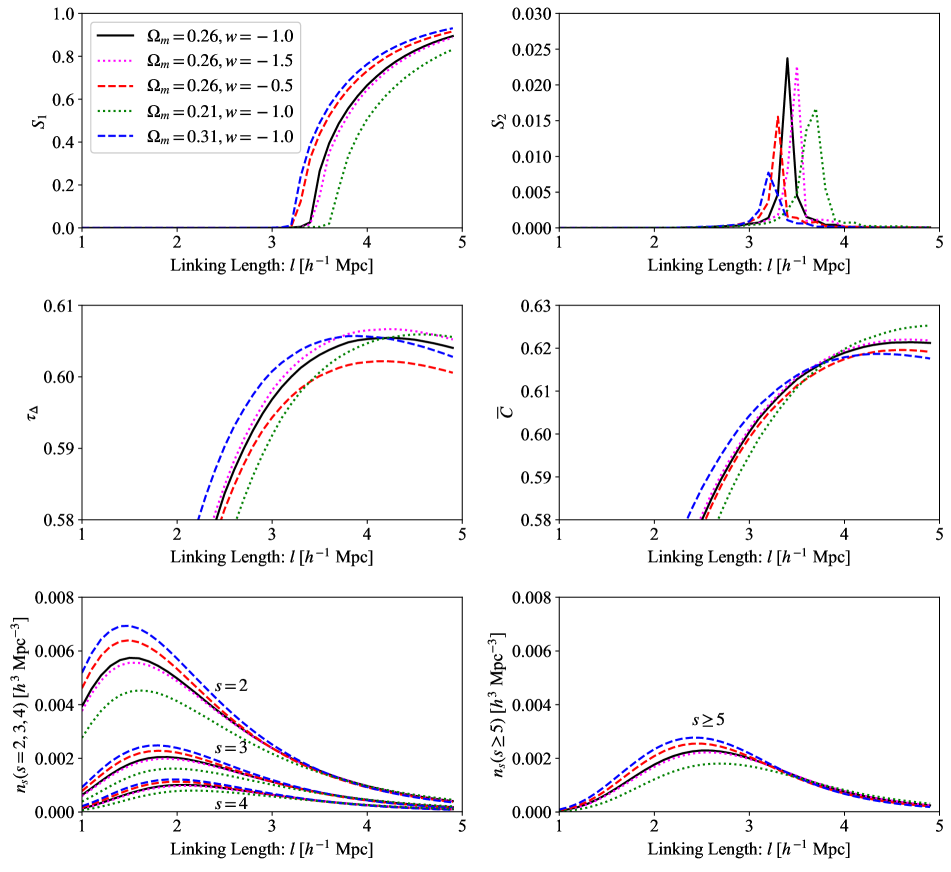
For the equal mass cut sample, as shown in Figure 6, all graph statistics are quite different enough to discern most of the Multiverses, except for the DE2 with $\Omega_{\rm m}=0.26,w=-1.5$ (dotted magenta lines). This model shows the least difference among the Multiverse suite from the standard universe in two-point statistics and abundances as shown in Figure 2 and Table 2; hence, the most elusive sample to discern statistically.

The spatial number density directly affects the percolation threshold and comoving densities of connected components. More points (vertices) in a fixed volume trivially make the percolation threshold shorter since the average distance between point pairs decreases. The comoving densities of connected components also increase due to the increment of overall point density. Hence, the top and bottom panels in Figure 6, showing the statistics of percolation and connected components, are significantly affected by the different abundances. When considering most of graph statistics are higher order measurements than the simple one-point statistic, any samples without matching abundances are very likely to show trivially different statistics in graph measurements.

4.1.2 Equal Abundance Sample: $N_{h}=7,086,717$

Figure 7: The same figure for the equal abundance sample, $N_{h}=7,086,717$, with Figure 6. We can observe that many graph statistics seem degenerate since the abundance effect is removed in this selection.

Figure 8: The residuals of graph statistics vs. the linking lengths for Figure 7. From STD-HR, we extract 27 subsamples with the volume of $1024^{3}h^{-3}$ Mpc³. The grey shaded area shows the residuals of these 27 subsamples, representing the cosmic variances of the standard universe in the Multiverse suite. The two statistics, $\tau_{\Delta}$ at most scales and $n_{s\geq 5}$ at the percolation threshold (vertical grey dotted line), seem the best discreminants for constraining cosmologies. We analyze the graph statistics in details at the percolation threshold in Figure 9.

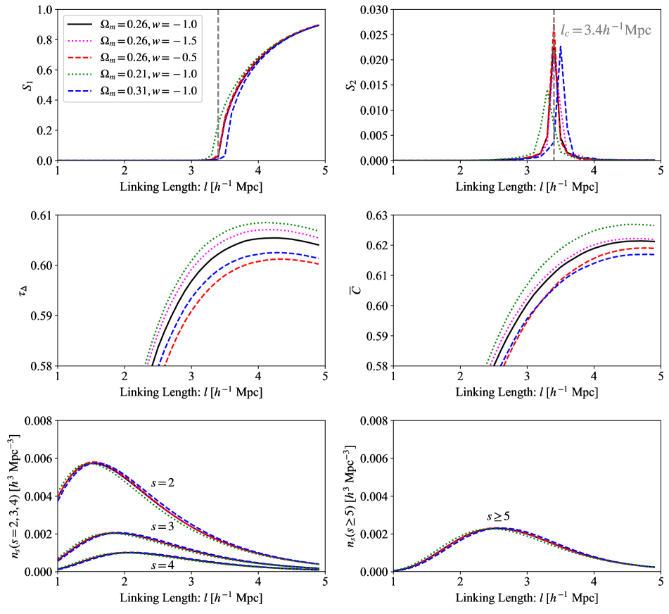
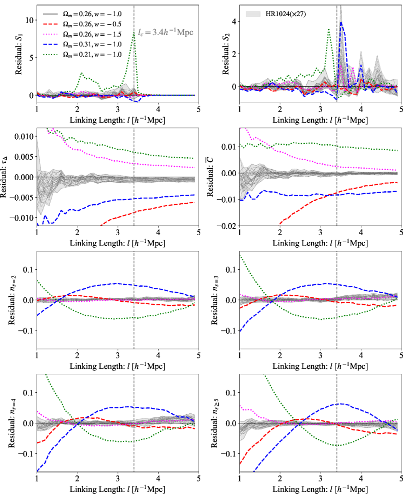
Figure 7 shows the graph statistics of equal abundance sample with $N_{h}=7,086,717$, of which comoving density is $n_{\rm h}=6.6\times 10^{-3}[h^{-1}$Mpc$]^{-3}$. Now, we can observe that many graph statistics seem degenerate since the abundance effect is removed in this selection; namely, a good testbed how well graph statistics can work as precise discriminators for constraining cosmology.

To better investigate these degenerate-looking features, we measure the residuals of graph statistics differing from the standard universe, shown in Figure 8. We also extract 27 subsamples with the volume of $V_{sub}=1024^{3}$ $[h^{-1}$Mpc$]^{3}$ from STD-HR and measure their residuals (grey lines; HR1024) to show the cosmic variances of graph statistics at this size of survey volume. The grey shaded area represents the range between the maximum and minimum residuals.

From the results shown in Figure 7 and 8, we can observe that each parameter variation (or, perturbation) of dark energy, $w=-0.5,-1.0,-1.5$, and dark matter , $\Omega_{\rm m}=0.21,0.26,0.31$, affects the graph topology of halo distributions in different ways. We describe this in details in the following two separate sections.

Percolation Threshold and Connected Components :
Degeneracy in Dark Energy Perturbation

In Figure 7, the top panels show the largest (left, $S_{1}$) and second largest connected subcomponent (right, $S_{2}$). Interestingly enough, the three models with equal $\Omega_{\rm m}=0.26$ show almost the same percolation curves in $S_{1}$ and $S_{2}$ statistics. The percolation thresholds of three models with $\Omega_{\rm m}=0.26$ are $l_{c}=3.4h^{-1}$Mpc, while those of $\Omega_{\rm m}=0.21$ and $0.31$ are smaller and larger than $l_{c}=3.4h^{-1}$Mpc. Hence, for the equal abundance sample, the percolation thresholds seem to only depend on $\Omega_{\rm m}$, ignoring the effects of various dark energy states.

As a comparison set, we calculate the percolation threshold, $l_{c}^{RGG}$, for RGG with $d=3$ using its critical threshold value, $\alpha_{c}=2.74$,

$$l_{c}^{RGG}(d=3) = \Big{(}\frac{3\alpha_{c}}{4\pi\bar{n}}\Big{)}^{\frac{1}{3}}$$ (27)

$$= 4.6h^{-1}\textrm{Mpc}$$

where $\bar{n}=6.6\times 10^{-3}\big{[}h^{-1}$Mpc$\big{]}^{-3}$. Since RGGs have zero correlation functions, the gaps, $|l_{c}-l_{c}^{RGG}|=1.2h^{-1}$ Mpc, in percolation thresholds between RGGs and Multiverse networks are caused by the contributions of all orders of non-zero correlation functions, as Zhang et al. (2018) have derived using their Probability Cloud Cluster Expansion Theory (PCCET). The generating function formulation in Equation 16, 17, and 18, also show the dependence of percolation threshold on $p_{k}$ with all orders of $k$, which implicitly reflects the dependence of all correlation functions.

The comoving densities of connected components ($n_{s=2}$, $n_{s=3}$, $n_{s=4}$, and $n_{s\geq 5}$) are shown in the bottom panels of Figure 7. Their residuals are plotted in the third and forth rows in Figure 8. The notable features are the $\cap$ and $\cup$ shapes for DM1 ($\Omega_{\rm m}=0.31$; blue dashes) and DM2 ($\Omega_{\rm m}=0.21$; green dots) near the percolation threshold, $l_{c}=3.4h^{-1}$Mpc, in the residual figure. In contrast, DE1 ($w=-0.5$; red lines) and DE2 ($w=-1.5$; magenta lines) are marginally separable when considering the cosmic variances (grey area). Hence, like the percolation thresholds, the comoving densities of connected components depend mainly on $\Omega_{\rm m}$ rather than $w$.

Finally, the locations of intersection between the red and magenta lines, where the effects of different dark energy parameters are nullified in the comoving densities of connected components, converge to the percolation threshold, $l_{c}=3.4h^{-1}$Mpc, as the connected component size, $s$, increases. For $n_{s\geq 5}$, we can observe that the intersecting point is located at the right percolation threshold. At this crossing point, the $\cap$ and $\cup$ residual features are, also, most prominent for $n_{s\geq 5}$. The other connected components, $n_{s=2}$, $n_{s=3}$, and $n_{s=4}$, show qualitatively the same results with $n_{s\geq 5}$. However, their crossing points between the red and magenta lines are located with offsets from the percolation threshold and the $\cap$ and $\cup$ residuals are less critical. Hence, $n_{s\geq 5}$ is the most preferred statistic to represent the properties of connected components as a cosmological discriminator.

Transitivity : Breaking the Degeneracy in Dark Energy Perturbation

The middle panels in Figure 7 show transitivity ($\tau_{\Delta}$; left) and local clustering coefficient ($\overline{C}$; right) for the equal abundance sample. Their residuals are plotted in the second row panels in Figure 8. Unlike the degenerate features of percolation properties, $l_{c}$ and $n_{s\geq 5}$, in the previous section, the two triangular statistics, $\tau_{\Delta}$ and $\overline{C}$, separate all Multiverses quite well.

As described in §3.3, $\overline{C}$ is a biased triangular density, while $\tau_{\Delta}$ an unbiased measurement. In addition, the residuals in Figure 8 are quite consistent for $\tau_{\Delta}$ in most linking lengths, while the residuals of $\overline{C}$ are not. Hence, though $\overline{C}$ is a still useful statistic, $\tau_{\Delta}$ is preferred to $\overline{C}$.

Overall, Figure 8 suggests that the two graph statistics, $\tau_{\Delta}$ and $n_{s\geq 5}$, measured at the percolation threshold, $l_{c}=3.4h^{-1}$Mpc, are the best statistics to discern different cosmology.

4.2 Simple Graph Diagnostics at Big Data Scales : $\alpha$, $\tau_{\Delta}$, $n_{s\geq 5}$

In the previous section, we have explored the graph properties of Multiverses and found that $\tau_{\Delta}$ and $n_{s\geq 5}$ measured at the percolation threshold are the best discriminators for constraining different cosmological parameters. In this section, we investigate diagnostic diagrams of graph statistics and their cosmic variances, depending on survey volume sizes, which determine the statistical precision of each diagram.

Figure 9: The graph diagnostics for the Multiverse samples at the percolation threshold, $l_{c}=3.4h^{-1}$Mpc. We split the total volume, $V^{1/3}=1024h^{-1}$ Mpc, into 64 subsamples with the volume of $V^{1/3}=256h^{-1}$ Mpc (right panels) and 8 subsamples with $V^{1/3}=512h^{-1}$ Mpc (middle panels). The single full-volume measurements, $V^{1/3}=1024h^{-1}$ Mpc, are shown in the left panels. From the implications obtained by these results, we suggest a diagnostic diagram in Figure 10 and present its statistical precision using finite-size scaling relations in Figure 11.

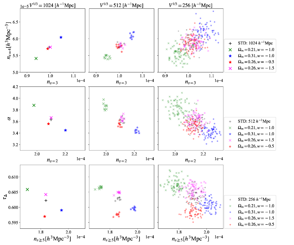
Figure 9 shows three diagnostic diagrams, $n_{s=4}$ vs. $n_{s=3}$ (top), $\alpha$ vs. $n_{s=2}$ (middle), and $\tau_{\Delta}$ vs. $n_{s\geq 5}$ (bottom), measured at the percolation threshold for three different volumes, $V^{1/3}=256$ (right), $512$ (middle), and $1024$ (left) $h^{-1}$Mpc. We split the total volume of Multiverse simulations, $V^{1/3}=1024$ $h^{-1}$Mpc, into 64 subsamples with $V^{1/3}=256$ $h^{-1}$Mpc and 8 subsamples with $V^{1/3}=512$ $h^{-1}$Mpc, which show roughly the cosmic variances for given subsample volumes in the diagnostic diagrams.

We can obtain various implications from the results in Figure 9. First, the cosmic variance of graph diagnostics for $V^{1/3}=256$ $h^{-1}$Mpc is too large to properly constrain the cosmological parameters. The second-column panels, roughly, suggest that we need a survey volume, $V^{1/3}\geq 512$ $h^{-1}$Mpc. Samplings in gigaparsecs scales will be necessary for more precise constraints. Therefore, graph analyses for constraining cosmology are inevitably a Big Data science. We will present the details about statistical precision of each graph statistic vs. data-size later in a separate paragraph. Second, the diagnostic diagrams of $n_{s=4}$ vs. $n_{s=3}$ (top panels) now clearly visualize the degeneracy of connected component statistics in dark energy perturbation, elaborately described in §4.1.2. Using $\alpha$ in the diagnostic diagram of $\alpha$ vs. $n_{s=2}$ (middle panels), we have a minor improvement for discerning the different dark energy parameters than the $n_{s=4}$ vs. $n_{s=3}$ diagram, but still this diagnostic diagram is not practically useful. Finally, as shown in Figure 8, the diagnostic diagrams of $\tau_{\Delta}$ vs. $n_{s\geq 5}$ (bottom panels) can separate all of the five Multiverses, though the survey volume of $V^{1/3}=256$ $h^{-1}$Mpc is still too small to constrain cosmology even in this diagnostic diagram. Consequently, including $\alpha$ as a proxy measurement of most commonly used two-point correlation function, we suggest a simple set of diagnostics, $\{\alpha,\tau_{\Delta},n_{s\geq 5}\}$, as a quick look of various orders of $n$-points correlation functions for cosmological Big Data sets.

Figure 10: The graph diagnostics of $\{\alpha,\tau_{\Delta},n_{s\geq 5}\}$ at the percolation threshold, $l_{c}=3.4h^{-1}$Mpc. Like Figure 8, we extract 27 subsamples with the volume of $1024^{3}h^{-3}$ Mpc³ from the Horizon Run data. The grey ‘+’ markers, referred to as STD-HR1024, show the graph statistics of these 27 subsamples, representing the cosmic variances of the diagnostics, which are quite small enough for accurately discerning all different Multiverses. The largest sample of STD-HR2048 is composed of 57 millions halos (vertices) with 206 millions connections (edges).

Figure 10 shows our final diagnostic diagrams, representing $\{\alpha,\tau_{\Delta},n_{s\geq 5}\}$. Except for the ‘Y’ marker, all data points are obtained using $V^{1/3}=1024$ $h^{-1}$Mpc; hence, samplings in a gigaparsec scale. The ‘Y’ marker, referred to as STD-HR2048, represents a single selection with $V^{1/3}=2048$ $h^{-1}$Mpc, extracted from STD-HR. This largest sample is composed of 57 millions halos (vertices) with 206 millions connections (edges). The grey ‘+’ makers, referred to as STD-HR1024$(\times 27)$, represent 27 subsamples with $V^{1/3}=1024$ $h^{-1}$Mpc, extracted from STD-HR, showing the cosmic variances of $\{\alpha,\tau_{\Delta},n_{s\geq 5}\}$ for the standard cosmology at the scale of $V^{1/3}=1024$ $h^{-1}$Mpc. The grey shaded area shown in Figure 8 is equivalent to these grey ‘+’ markers.

From the diagnostics diagrams in Figure 10, we can distinguish the most elusive sample, DE2, with $\Omega_{\rm m}=0.26,w=-1.5$ (magenta ‘x’), from the standard universe (black ‘+’) with a high statistical precision. In the $\tau_{\Delta}$ vs. $n_{s\geq 5}$ diagnostics (left panel), the dark energy perturbation moves the graph statistics vertically from the standard universe due to the degenerate statistics in percolation and connected components. On the other hand, the dark matter, the dominant content for $\Omega_{\rm m}$, perturbation changes all statistics, resulting in moving the graph statistics in the oblique axis from the standard universe.

Since gravity is an all-range force, the variation of $\Omega_{\rm m}$ affects all scales of matter distributions. This unique property of gravity changes all graph statistics as shown in many figures through this paper. However, since dark energy only expands the space, the effect of dark energy variation should be limited, when compared to the effect of gravity. In the graph statistics, this limitation of dark energy is observed as the degenerate statistics in percolation and connected components. Due to this difference, each parameter perturbation moves the graph statistics along different axis as shown in Figure 10.

Figure 11: The means and standard deviations of $\{\alpha,\tau_{\Delta},n_{s\geq 5}\}$ for various volume sizes at the percolation threshold, $l_{c}=3.4h^{-1}$Mpc. The numbers of sub-samples for $V^{1/3}$ = 256, 362, 512, 724, and 1024 $h^{-1}$Mpc are $1728$, $512$, $216$, $64$, and $27$ respectively. The ‘Y’ marker represents STD-HR2048, also shown in Figure 10. In the left panels, we fit the mean values for each statistic using the finite-size scaling function. In the right panels, from the $V^{1/3}=256h^{-1}{\rm Mpc}$ results we extrapolate the standard deviation values following the scaling relation, $\propto\frac{1}{\sqrt{V}}$ (i.e., $\propto L^{-1.5}$), plotted as grey dotted lines. Overall, the effects of survey volume sizes are well predictable by finite-size scaling relations with Poissonian variances. Notably, this scaling analysis is virtually impossible without modern Big Data tools.

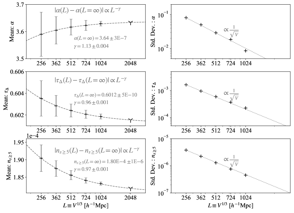
Figure 11 shows how each graph quantity depends on volume sizes for Horizon Run, the largest simulation box. The numbers of subsamples for $L\equiv V^{1/3}$ = 256, 362, 512, 724, and 1024 $h^{-1}$Mpc are $1728$, $512$, $216$, $64$, and $27$ respectively. In the right panels, we extrapolate the standard deviation values from the results at $V^{1/3}=256h^{-1}{\rm Mpc}$, following the scaling relation, $\propto\frac{1}{\sqrt{V}}$ (i.e., $\propto L^{-1.5}$; grey dotted lines). The measured standard deviations (hence, the cosmic variances; ‘+’ markers) of the graph diagnostics, $\{\alpha,\tau_{\Delta},n_{s\geq 5}\}$, follow this scaling relation, $\propto\frac{1}{\sqrt{V}}$, quite well.

For the mean values of $\{\alpha,\tau_{\Delta},n_{s\geq 5}\}$, we fit them using the scaling relation,

$$|\eta(L)-\eta(L=\infty)|\propto L^{-\gamma},$$ (28)

where $\eta(L)$ is one of $\{\alpha,\tau_{\Delta},n_{s\geq 5}\}$ at the system size, $L\equiv V^{1/3}$. This scaling relation is also known as finite-size scaling in statistical physics. We rewrite Equation 28 in a more practical form as,

$$\eta(L)=\epsilon\Big{(}\frac{L}{L_{0}}\Big{)}^{-\gamma}+\eta_{0}-\epsilon,$$ (29)

where $\eta_{0}=\eta(L_{0})$ and $\eta(L=\infty)=\eta_{0}-\epsilon$. The left panels of Figure 11 show the scaling exponents and asymptotic values by using the fitting function, Equation 29, with $L_{0}=2048h^{-1}{\rm Mpc}$. Consequently, the effects of survey volume sizes on the graph diagnostics, $\{\alpha,\tau_{\Delta},n_{s\geq 5}\}$, are well predictable by finite-size scaling relations with Poissonian variances. Notably, this scaling analysis is virtually impossible without modern Big Data tools.

5 Summary and Discussion

By utilizing the modern Big Data platform, Apache Spark, we have investigated the graph topology of discrete point distributions of dark matter halos for five different universes; a suite of Multiverse simulations, (1) STD: $\Omega_{\rm m}=0.26,w=-1.0$, (2) DE1: $\Omega_{\rm m}=0.26,w=-0.5$, (3) DE2: $\Omega_{\rm m}=0.26,w=-1.5$, (4) DM1: $\Omega_{\rm m}=0.31,w=-1.0$, and (5) DM2: $\Omega_{\rm m}=0.21,w=-1.0$. The equal mass cut sample, selecting halos above $M_{\rm cut}=5\times 10^{11}h^{-1}$M_⊙, shows quite different graph statistics, mainly due to their different abundances, which affect graph measurements significantly. Hence, it is trivial to discern all of the five different Multiverses using graph statistics in this equal mass cut selection.

The equal abundance sample, selecting halos using $N_{h}=7,086,717$ of which comoving density is $n_{\rm h}=6.6\times 10^{-3}$ $[h^{-1}$Mpc$]^{-3}$, show degenerate statistics in percolation threshold and connected components for STD, DE1, and DE2. This means that the graph statistics related to percolation, $\{n_{s=2}$, $n_{s=3}$, $n_{s=4}$, $n_{s\geq 5}$, $l_{c}\}$, mostly depend on $\Omega_{\rm m}$, not $w$.

The degenerate percolation threshold for STD, DE1, and DE2 is $l_{c}=3.4h^{-1}$Mpc, different from their corresponding RGG, $l_{c}^{RGG}=4.6h^{-1}$Mpc. Since RGG has zero correlation functions, the difference in percolation thresholds, $|l_{c}-l_{c}^{RGG}|=1.2h^{-1}$Mpc, between RGG and Multiverse networks is caused by the non-zero correlation functions of all orders.

This degeneracy can be removed by the triangular statistics, $\tau_{\Delta}$ and $\overline{C}$. Among all graph statistics measured in this paper, $\tau_{\Delta}$ and $n_{s\geq 5}$ are the best discriminators for constraining cosmology. By including $\alpha$ as a proxy of most commonly used statistic, two-point correlation function, we have suggested a graph diagnostics set, $\{\alpha$, $\tau_{\Delta}$, $n_{s\geq 5}\}$, as a quick look of various orders of correlation functions at Big Data scales in a computationally cheap way. Using the finite-size scalings, we have shown that the cosmic means and variances of $\alpha$, $\tau_{\Delta}$, and $n_{s\geq 5}$ are well described by various power-laws.

Future research will investigate the practical observable, galaxies, at Big Data scales since the obvious caveat of this work is the FoF halo catalogs, which lack for complex and sophisticated baryonic physics in formation and evolution of galaxies. As Hong et al. (2019) have reported a transitivity anomaly in Lyman alpha emitting galaxies (LAEs), implying a strong environmental effect on formation and evolution of LAEs, graph statistics of galaxy catalogs are inevitably affected by baryonic physics, which could erase the underlying cosmological parameters. Hence, we may need to extract more topological features from galaxy catalogs for better constraining cosmology using the state-of-the-art graph analyses. Technically, this means that we need to fully utilize both of single machine and distributed computing Application Programming Interfaces (APIs). The single machine APIs support many feature extractions, but limited to small data sets fit in a single machine, while the distributed computing APIs support limited feature extractions, but can handle big data sets. Therefore, galaxy catalogs at Big Data scales will be a good challenge to fully test the current state-of-the-art graph analyses tools.

References

- Albert & Barabási (2002) Albert, R., & Barabási, A.-L. 2002, Rev. Mod. Phys., 74, 47, doi: 10.1103/RevModPhys.74.47
- Aragón-Calvo et al. (2007) Aragón-Calvo, M. A., Jones, B. J. T., van de Weygaert, R., & van der Hulst, J. M. 2007, A&A, 474, 315, doi: 10.1051/0004-6361:20077880
- Ata et al. (2018) Ata, M., Baumgarten, F., Bautista, J., et al. 2018, MNRAS, 473, 4773, doi: 10.1093/mnras/stx2630
- Barrow et al. (1985) Barrow, J. D., Bhavsar, S. P., & Sonoda, D. H. 1985, MNRAS, 216, 17, doi: 10.1093/mnras/216.1.17
- Barthélemy (2011) Barthélemy, M. 2011, Phys. Rep., 499, 1, doi: 10.1016/j.physrep.2010.11.002
- Bond et al. (2010) Bond, N. A., Strauss, M. A., & Cen, R. 2010, MNRAS, 409, 156, doi: 10.1111/j.1365-2966.2010.17307.x
- Cautun et al. (2013) Cautun, M., van de Weygaert, R., & Jones, B. J. T. 2013, MNRAS, 429, 1286, doi: 10.1093/mnras/sts416
- Colberg (2007) Colberg, J. M. 2007, MNRAS, 375, 337, doi: 10.1111/j.1365-2966.2006.11312.x
- Dall & Christensen (2002) Dall, J., & Christensen, M. 2002, Phys. Rev. E, 66, 016121, doi: 10.1103/PhysRevE.66.016121
- Dorogovtsev et al. (2008) Dorogovtsev, S. N., Goltsev, A. V., & Mendes, J. F. F. 2008, Reviews of Modern Physics, 80, 1275, doi: 10.1103/RevModPhys.80.1275
- Dubinski et al. (2004) Dubinski, J., Kim, J., Park, C., & Humble, R. 2004, New Astronomy, 9, 111, doi: 10.1016/j.newast.2003.08.002
- Dunkley et al. (2009) Dunkley, J., Komatsu, E., Nolta, M. R., et al. 2009, ApJS, 180, 306, doi: 10.1088/0067-0049/180/2/306
- Eisenstein et al. (1998) Eisenstein, D. J., Hu, W., & Tegmark, M. 1998, The Astrophysical Journal, 504, L57, doi: 10.1086/311582
- Eisenstein et al. (2005) Eisenstein, D. J., Zehavi, I., Hogg, D. W., et al. 2005, ApJ, 633, 560, doi: 10.1086/466512
- Eriksen et al. (2004) Eriksen, H. K., Novikov, D. I., Lilje, P. B., Banday, A. J., & Górski, K. M. 2004, ApJ, 612, 64, doi: 10.1086/422570
- Gott et al. (1987) Gott, III, J. R., Weinberg, D. H., & Melott, A. L. 1987, ApJ, 319, 1, doi: 10.1086/165427
- Hong et al. (2016) Hong, S., Coutinho, B. C., Dey, A., et al. 2016, MNRAS, 459, 2690, doi: 10.1093/mnras/stw803
- Hong & Dey (2015) Hong, S., & Dey, A. 2015, MNRAS, 450, 1999, doi: 10.1093/mnras/stv722
- Hong et al. (2019) Hong, S., Dey, A., Lee, K.-S., et al. 2019, MNRAS, 483, 3950, doi: 10.1093/mnras/sty3219
- Huchra & Geller (1982) Huchra, J. P., & Geller, M. J. 1982, ApJ, 257, 423, doi: 10.1086/160000
- Hwang et al. (2016) Hwang, H. S., Geller, M. J., Park, C., et al. 2016, ApJ, 818, 173, doi: 10.3847/0004-637X/818/2/173
- Kim et al. (2015) Kim, J., Park, C., L’Huillier, B., & Hong, S. E. 2015, Journal of Korean Astronomical Society, 48, 213, doi: 10.5303/JKAS.2015.48.4.213
- Levi et al. (2013a) Levi, M., Bebek, C., Beers, T., et al. 2013a, ArXiv e-prints. https://arxiv.org/abs/1308.0847
- Levi et al. (2013b) —. 2013b, ArXiv e-prints. https://arxiv.org/abs/1308.0847
- Martinez et al. (2005) Martinez, V. J., Starck, J.-L., Saar, E., et al. 2005, The Astrophysical Journal, 634, 744, doi: 10.1086/497125
- Newman (2003) Newman, M. 2003, SIAM Review, 45, 167, doi: 10.1137/S003614450342480
- Park et al. (2013) Park, C., Pranav, P., Chingangbam, P., et al. 2013, Journal of Korean Astronomical Society, 46, 125, doi: 10.5303/JKAS.2013.46.3.125
- Planck Collaboration et al. (2016a) Planck Collaboration, Ade, P. A. R., Aghanim, N., et al. 2016a, A&A, 594, A13, doi: 10.1051/0004-6361/201525830
- Planck Collaboration et al. (2016b) —. 2016b, A&A, 594, A17, doi: 10.1051/0004-6361/201525836
- Plaszczynski et al. (2018) Plaszczynski, S., Peloton, J., Arnault, C., & Campagne, J. E. 2018, arXiv e-prints, arXiv:1807.03078. https://arxiv.org/abs/1807.03078
- Pranav et al. (2017) Pranav, P., Edelsbrunner, H., van de Weygaert, R., et al. 2017, MNRAS, 465, 4281, doi: 10.1093/mnras/stw2862
- Sheth et al. (2003) Sheth, J. V., Sahni, V., Shandarin, S. F., & Sathyaprakash, B. S. 2003, MNRAS, 343, 22, doi: 10.1046/j.1365-8711.2003.06642.x
- Shoji et al. (2009) Shoji, M., Jeong, D., & Komatsu, E. 2009, ApJ, 693, 1404, doi: 10.1088/0004-637X/693/2/1404
- Sousbie et al. (2007) Sousbie, T., Pichon, C., Courtois, H., Colombi, S., & Novikov, D. 2007, The Astrophysical Journal, 672, L1, doi: 10.1086/523669
- Takahashi (2014) Takahashi, T. 2014, Progress of Theoretical and Experimental Physics, 2014, doi: 10.1093/ptep/ptu060
- van de Weygaert et al. (2013) van de Weygaert, R., Vegter, G., Edelsbrunner, H., et al. 2013, arXiv e-prints, arXiv:1306.3640. https://arxiv.org/abs/1306.3640
- Zaharia (2014) Zaharia, M. 2014, PhD thesis, EECS Department, University of California, Berkeley. http://www2.eecs.berkeley.edu/Pubs/TechRpts/2014/EECS-2014-12.html
- Zhang et al. (2018) Zhang, J., An, R., Liao, S., et al. 2018, Phys. Rev. D, 98, 103530, doi: 10.1103/PhysRevD.98.103530