Experimental Challenges of Implementing Quantum Phase Estimation Algorithms on IBM Quantum Computers

Abstract

Quantum phase estimation (QPE) is the core of the most quantum algorithms which is mainly used for algorithm such as Shor’s factoring algorithm, quantum sampling algorithm and finding the eigenvalues of unitary matrices. Several algorithms like inverse Quantum Fourier transform and Kitaev’s algorithms are used to implement QPE and extract the unknown phase. In this paper, different algorithms for implementing quantum phase estimation are explained, modeled by the simulator and, experimentally tested by actual IBM quantum machine. Implementation of these algorithms are constrained by several challenges. We explained these challenges and the solutions to improve the accuracy of the implementation output.

I INTRODUCTION

Quantum computers can provide a framework to solve problems very fast in comparison with classical computers. These days, remarkable progress, different technologies are being provided by different companies to implement the classical algorithms using quantum computers. Classical computers works based on a Load-Run-Read cycle in which the input data load into the system, a program runs and then the output of the program is read. However, in quantum computers there is Prepare-Evolve-Measure cycle wherein the quantum states are prepare as the input, evolve the input in quantum computers using the operators and then the results are measured. [1]. The computational power of quantum computers comes from the use of superposition and entanglement of the qubits. Phase estimation is the important part of most known quantum algorithms like developing Shor’s algorithm for factoring the prime numbers, quantum chemistry to model the molecules and, Grover’s algorithm to search [2, 3, 4, 5, 6, 7, 8]. Phase estimation is The main part of Shor’s algorithm for factoring algorithm [4]. This algorithm was implemented by different quantum computers. Implementing Shor’s algorithm for factoring 15 (which is 3*5) on a nuclear magnetic resonance (NMR) computer was presented in [9]. In [10] the number 21 was factored by implementing qubit recycling in a photonic circuit. The largest number that has been factored by actual quantum computer is the number 143 and implemented on a dipolar coupling NMR System by applying adiabatic quantum computation[11]. The goal of quantum phase estimation is to determine the eigenvalues of a unitary matrix with an unchanged eigenvector. Two main approaches are used to implement quantum the phase estimation. (1) extract the phase information by applying the classical post processing after quantum gate operations (Kitaev’s algorithm) [12, 13] and (2) Quantum Fourier transform based approach in which the phase is estimated by applying quantum inverse Fourier Transform[14, 18, 15]. The QFT algorithm requires large number of rotation gates to extract the information about the phase with more precision digits however implementing the technique in actual quantum computer increase the output error. The goal is to extract the phase with less depth and controlled-rotation gates. An experimental phase estimation based on quantum Fourier transform was implemented on a three-bit nuclear magnetic resonance (NMR) processor [16] However, it as only used to estimate the eigenvalues of one-bit Grover operators. [17] proposed an implementation of phase estimation algorithm to find the eigenstates of the system by applying on a ion trap quantum computer. Recently Lloyd and co-authors have been shown that by applying quantum phase estimation technique the speed of some linear algebraic techniques applied in machine learning algorithm like principle component (PCA), support vector machine (SVM) and k-means can be improved by quantum computers.[19, 20] However, implementing these techniques in actual quantum machine and, the error correction have not yet provided.

In this paper different phase estimation algorithms are analyzed, simulated and experimentally tested in a 20 qubits IBM quantum machine. We demonstrate that there exist challenges in implementing quantum algorithm in actual quantum computer. Increasing number of qubits and quantum operations add more the error to the system and as a result diverge the correct answer. In order to improve the accuracy of the system different techniques are used to decrease the number of controlled-gate and phase shift operators and therefore the system converge to the correct answer.

This paper is categorized as follows. Section II describes the basic operation and various phase estimation algorithm. In section III Kitaev’s algorithm is explained, modeled. Section IV provides an iterative algorithm to estimate the phase. LLoyd algorithm for phase estimation based on inverse Fourier transform (QFT) is describes in section V. In section VI the simulation and experimental result for each method is provided and compared. Finally, the conclusion of the paper is summarized in Section VII.

II Phase estimation

Quantum phase estimation of an unitary matrix mainly can be derived using two methods, (1) applying the inverse Quantum Fourier Transform (QFT) to derived the information about the unknown phase and (2) sequential post processing techniques to calculate the unknown phase. Phase estimation technique is used to estimate the eigenvalues $\ket{\lambda}$ of an unitary matrix $U$ with its known eigenvector $\ket{\psi_{\lambda}}$, [21]

$$U\ket{\psi_{\lambda}}=\lambda\ket{\psi_{\lambda}}$$ (1)

Where eigenvalues of the unitary matrix is $\lambda=e^{2\pi i\varphi_{m}}$. The goal of phase estimation is to find the eigenvalues of the unitary matrix and apply them to estimate the unknown phase of the unitary operator. $\varphi_{k}=0.x_{1}x_{2}x_{3}...x_{n}$ is the phase of unitary matrix that needs to be estimated. The estimated variable $(\hat{\varphi})$ can be expressed as binary representation,

$$\hat{\varphi}=\frac{x_{1}}{2}+\frac{x_{2}}{2^{2}}+\frac{x_{3}}{2^{3}}+\cdot\cdot\cdot+\frac{x_{n}}{2^{n}}$$ (2)

By applying the quantum circuit that can transform the states on the unitary matrix the required information about the phase can not be achieved. Fig.1 shows the quantum circuit applied to one qubit and eigenstate. As can be seen the output of the circuit contains the phase but, due to the superposition on the value, finding the phase using this circuit is not possible. In order to estimate the phase different techniques are applied to provide the information about the phase of the system. In the next sections we will explain these techniques along with their simulated and experimentally implemented results.

Figure 1: Quantum circuit for transforming the states

Figure 2: Controlled U circuit

III Kitaev’s Algorithm

Kitaev’s algorithm is the first algorithm that was introduced to estimate the phase of an unitary matrix. In this technique a set of Hadamard gates are applied to the input qubits, the outputs of Hadamard gate are performed with Controlled-$U^{2^{k-1}}$ to implement the phase shift operator. Applying controlled $U$ operator k times transforms the control qubit to $\frac{1}{\sqrt{2}}\big{(}\ket{0}+e^{-i2\pi\varphi_{k}2^{k-1}}\ket{1}\big{)}$. At each test phase $\varphi_{k}=2^{k-1}\varphi$ can be calculated. By doing k times test and measuring the output of each test the set of values ${\varphi,2\varphi,\cdot\cdot\cdot,2^{k-1}\varphi}$ can be achieved. These measurements are used to estimate the phase of the unitary matrix. Fig.2 shows the circuit to perform phase estimation. As can be seen for the circuit operation K can be used to manipulate the qubit phase and provides more information about the phase of the system. Considering $K=I_{2}$, the quantum circuit provide the following analysis,

$$\begin{array}[]{l}\ket{0}\ket{\psi_{\lambda}}\enspace\>\xrightarrow{H\bigotimes I}\qquad\frac{1}{\sqrt{2}}(\ket{0}+\ket{1})\ket{\psi_{\lambda}}\\ \\ \qquad\qquad\xrightarrow{C-U_{k}}\qquad\frac{1}{\sqrt{2}}(\ket{0}+\ket{1})\bigotimes U_{k}\ket{\psi_{\lambda}}\\ \\ \qquad\qquad=\frac{1}{\sqrt{2}}(\ket{0}\ket{\psi_{\lambda}}+e^{2\pi i\varphi_{k}}\ket{1}\ket{\psi_{\lambda}})\\ \\ \quad\xrightarrow{H\bigotimes I}\qquad\frac{1}{\sqrt{2}}\frac{\big{(}\ket{0}+\ket{1}\big{)}}{\sqrt{2}}\ket{\psi_{\lambda}}+\frac{e^{2\pi i\varphi_{k}}}{\sqrt{2}}\frac{\big{(}\ket{0}-\ket{1}\big{)}}{\sqrt{2}}\ket{\psi_{\lambda}}\\ \\ \qquad\qquad=\frac{1}{2}\bigg{(}\big{(}1+e^{2\pi i\varphi_{k}}\big{)}\ket{0}+\big{(}1-e^{2\pi i\varphi_{k}}\big{)}\ket{1}\bigg{)}\ket{\psi_{\lambda}}\par\par\end{array}$$ (3)

Based on the calculations from Eq.3, the probability of measuring $\ket{0}$ and $\ket{1}$ will be,

$$P(0|k)=\frac{1+cos(2\pi\varphi_{k})}{2},\qquad P(1|k)=\frac{1-cos(2\pi\varphi_{k})}{2}$$ (4)

$\varphi_{k}$ can be obtained with more precise estimated digit by applying more trials. However, based on the data from Eq. 3 we cannot distinguish between $\varphi_{k}$ and $-\varphi_{k}$. In order to solve this problem another circuit is required to be considered to provide more information about the phase of the unitary matrix. Combination of the results from $K=I_{2}$ and $K=S$ helps to find the actual value of the phase. In a case that $K=S$ gate is used and applied in the circuit, the analysis will be,

$$K=S=\begin{pmatrix}1&0\\ 0&i\end{pmatrix}$$ (5)

Quantum circuit provides the following transformation,

$$\begin{array}[]{l}\ket{0}\ket{\psi_{\lambda}}\enspace\>\xrightarrow{H\bigotimes I}\qquad\frac{1}{\sqrt{2}}(\ket{0}+\ket{1})\ket{\psi_{\lambda}}\\ \\ \>\qquad\qquad\xrightarrow{S}\qquad\enspace\enspace\>\frac{1}{\sqrt{2}}(\ket{0}+i\ket{1})\ket{\psi_{\lambda}}\\ \qquad\qquad\xrightarrow{C-U_{k}}\qquad\frac{1}{\sqrt{2}}(\ket{0}+i\ket{1})\bigotimes U_{k}\ket{\psi_{\lambda}}\\ \\ \qquad\qquad=\frac{1}{\sqrt{2}}(\ket{0}\ket{\psi_{\lambda}}+ie^{2\pi i\varphi_{k}}\ket{1}\ket{\psi_{\lambda}})\\ \end{array}$$ (6)

$$\begin{array}[]{l}\qquad\quad\xrightarrow{H\bigotimes I}\qquad\frac{1}{\sqrt{2}}\frac{\big{(}\ket{0}+i\ket{1}\big{)}}{\sqrt{2}}\ket{\psi_{\lambda}}+i\frac{e^{2\pi i\varphi_{k}}}{\sqrt{2}}\frac{\big{(}\ket{0}-i\ket{1}\big{)}}{\sqrt{2}}\ket{\psi_{\lambda}}\\ \\ =\frac{1}{2}\bigg{(}\big{(}1+ie^{2\pi i\varphi_{k}}\big{)}\ket{0}+\big{(}1-ie^{2\pi i\varphi_{k}}\big{)}\ket{1}\bigg{)}\ket{\psi_{\lambda}}\\ =\frac{1}{2}\bigg{(}\big{(}1+e^{2\pi i\varphi_{k}+\frac{\pi}{2}}\big{)}\ket{0}+\big{(}1-ie^{2\pi i\varphi_{k}+\frac{\pi}{2}}\big{)}\ket{1}\bigg{)}\ket{\psi_{\lambda}}\par\end{array}$$ (7)

The probabilities in this case will be,

$$P(0|k)=\frac{1-sin(2\pi\varphi_{k})}{2},\qquad P(1|k)=\frac{1+sin(2\pi\varphi_{k})}{2}$$ (8)

Eq.8 provides more information about the phase that helps to recover the phase of the unitary matrix. In each test the probabilities of being zero or one in $t$ trials are measured. By using the result from Eq.4 and Eq.8 the estimation of $cos(2\pi\varphi_{k})$ and $sin(2\pi\varphi_{k})$ and as a result hase $(\hat{\varphi})$ can be calculated as,

$$\hat{\varphi_{k}}=\frac{1}{2\pi}\;tan^{-1}\bigg{(}\frac{C_{k}}{S_{k}}\bigg{)}$$ (9)

Where $C_{k}$ and $S_{k}$ are the estimation of $cos(2\pi\varphi_{k})$ and $sin(2\pi\varphi_{k})$ respectively. In Kitaev’s algorithm post processing calculation is required to estimate the value of the phase. Estimating of the phase within $m$ bits of accuracy requires to increase the number of trials. $O\big{(}\frac{log(1-\delta)}{\epsilon_{2}}\big{)}$ samples are required to estimate within $\epsilon$ with probability of $1-\delta$.

TABLE I: Iterative Quantum phase estimation

IV Iterative Quantum Phase estimation

In the experimental implementation, increasing the number of gate to estimate the phase with higher accuracy will increase the convergence error and approach to a wrong answer. In this section an iterative technique was proposed to implement the Kiteav’s algorithm with higher accuracy and applying two qubits. This sequential approach helps to find the unknown phase of the system with $m$ bits of accuracy. Table I shows the the proposed algorithm. As it can be seen, one Hadamard gate was used to perform the superposition and then U-controlled gate is applied to the output of the Hadamard gate then, the output of this stage transform to the measurment state by applying another Hadamard gate. In the next iteration the order of Controlled-U gate is updated and the result from the previous measurement was used and applied to the circuit to estimate the new bit. This technique was repeated $m$ times to estimate the phase with m bits of accuracy. In this method in each iteration the information from the previous iterations were used to estimated the nest bit of the phase

V Phase estimation based on inverse QFT

One of the common method that is used to implement QPE is based on inverse QFT. The general view of this method has been shown in Fig.3. In this method two stages are required for phase estimation. First stage starts with n-qubits initialized at $\ket{0}$, prepares the state $\ket{psi}$ and, the second stage uses inverse quantum Fourier transform operation to estimate the binary digits of the phase. The mathematical analysis of the first stage is as,

$$\begin{array}[]{l}\frac{1}{\sqrt{2}}\big{(}\ket{0}+e^{2\pi i2^{n-1}\varphi}\ket{1}\big{)}\frac{1}{\sqrt{2}}\big{(}\ket{0}+e^{2\pi i2^{n-2}\varphi}\ket{1}\big{)}\cdot\cdot\cdot\\ \frac{1}{\sqrt{2}}\big{(}\ket{0}+e^{2\pi i\varphi}\ket{1}\big{)}=\frac{1}{2^{n/2}}\sum_{k=0}^{2^{n-1}}{e^{2\pi i\frac{\varphi k}{2^{n}}}\ket{k}}\end{array}$$ (10)

considering $\varphi=x/2^{n}$ where $x=\sum_{i=0}^{n-1}{2^{i}x_{i}}$ we have,

$$\begin{array}[]{l}\frac{1}{\sqrt{2}}\big{(}\ket{0}+e^{2\pi i0.x_{n}}\ket{1}\big{)}\frac{1}{\sqrt{2}}\big{(}\ket{0}+e^{2\pi i0.x_{n-1}x_{n}\varphi}\ket{1}\big{)}\cdot\cdot\cdot\\ \frac{1}{\sqrt{2}}\big{(}\ket{0}+e^{2\pi i0.x_{1}x_{2}...x_{n}}\ket{1}\big{)}=\frac{1}{2^{n/2}}\sum_{k=0}^{2^{n-1}}{e^{2\pi i\frac{\varphi k}{2^{n}}}\ket{k}}\end{array}$$ (11)

As can be seen form Fig.3 the outputs from the first stage (phase Kick-back) are the input of inverse QFT. By applying controlled-$U^{2^{n-1}}$ there will phase kick back to prepare the states. Also, the output of the first stage is exactly quantum Fourier transform of $\varphi$. By applying the inverse QFT we can recover the unknown phase. In order to analyze this method two different phase estimation circuit with different accuracy have been considered,

Figure 3: Quantum Phase estimation based on inverse Quantum Fourier Transform (QFT)

Figure 4: one bit phase estimation Quantum circuit

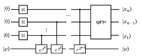
Case1: Considering $\varphi$ = $0.x_{1}$, the circuit shown in Fig. 4 and applying Hadamard gate to the initial state $\ket{0}$ we have:

$$\begin{array}[]{l}\ket{0}\enspace\>\xrightarrow{H}\qquad\frac{1}{\sqrt{2}}\big{(}\ket{0}+\ket{1}\big{)}\\ \qquad\xrightarrow{U}\qquad\frac{1}{2}\big{(}\ket{0}+e^{2\pi i\varphi}\big{)}\ket{1}\\ \qquad\xrightarrow{H}\qquad\frac{1}{2}\big{(}1+e^{2\pi i\varphi}\big{)}\ket{0}+\big{(}1-e^{2\pi i\varphi}\big{)}\ket{1}\\ \qquad\qquad=\frac{1}{2}\big{(}1+e^{2\pi i0.x_{1}}\big{)}\ket{0}+\big{(}1-e^{2\pi i0.x_{1}}\big{)}\ket{1}\\ \end{array}$$ (12)

Calculating the probability from equation (12) we have,

$$\begin{array}[]{l}P(\ket{0})=\frac{1+cos(2*\pi*0.x_{1})}{2},\qquad P(\ket{1})=\frac{1-cos(2*\pi*0.x_{1})}{2}\par\par\end{array}$$ (13)

Based on the result from equation (13), if $x_{1}=0$, then the probability of $\ket{0}$ is $1$ ($P(\ket{0})=1$) and if $x_{1}=1$, then the probability of $\ket{1}$ is $1$ ($P(\ket{1})=1$). It means that in a case that phase is considered as one bit only one Hadamard gate is required to extract $x_{1}$.

Case2: Considering $\varphi$ = $0.x_{1}x_{2}$, implementing circuit in Fig.5 and, applying Hadamard gate we have:

$$R_{k}=\begin{pmatrix}1&0\\ 0&e^{2\pi i/2^{k}}\end{pmatrix}$$ (14)

$$\begin{array}[]{l}\ket{0}\enspace\>\xrightarrow{H}\qquad\frac{1}{\sqrt{2}}\big{(}\ket{0}+\ket{1}\big{)}\\ \qquad\xrightarrow{U}\qquad\frac{1}{2}\big{(}\ket{0}+e^{2\pi i\varphi}\big{)}\ket{1}\\ \qquad\xrightarrow{H}\qquad\frac{1}{2}\big{(}1+e^{2\pi i\varphi}\big{)}\ket{0}+\big{(}1-e^{2\pi i\varphi}\big{)}\ket{1}\\ \qquad\qquad=\frac{1}{2}\big{(}1+e^{2\pi i0.x_{1}}\big{)}\ket{0}+\big{(}1-e^{2\pi i0.x_{1}}\big{)}\ket{1}\\ \end{array}$$ (15)

Calculating the probability from equation (15) we have,

$$\begin{array}[]{l}P(\ket{0})=\frac{1+cos(2*\pi*0.x_{1})}{2},\qquad P(\ket{1})=\frac{1-cos(2*\pi*0.x_{1})}{2}\par\par\end{array}$$ (16)

Based on equation (13), if $x_{1}=0$, then the probability of $\ket{0}$ is $1$ and if $x_{1}=0$, then the probability of $\ket{1}$ is 1. It means that only using one Hadamard gate can help to extract $x_{1}$. Fig.4 show the circuit for extracting $x_{1}$ in this case.

Figure 5: 3-Qubits inverse Quantum Fourier Transform (QFT)

VI Experimental and simulation Implementation

VI-A Simulation Results

In this paper, we show not only how to implement Quantum Phase Estimation Algorithms (QPEAs) on IBM quantum computers but also how to increase the accuracy of experimental results by carefully designing quantum gates for algorithms and taking advantages of classical computers to store intermittent results for future operations. Our simulation results demonstrate that physical errors from noisy quantum devices can be significantly reduced by carefully designing quantum gates for QPEAs with the help of classical computers. For example, we found that single qubit in IBM Q experience has good fidelity on quantum operations. However, the fidelity will be dramatically decreased as the number of control qubits increases.

Figure 6: Kitaev Quantum Phase Estimation Algorithm on Simulator and IBM Tokyo QX

Figure 7: Iterative Quantum Phase Estimation Algorithm on Simulator and IBM Tokyo QX

VI-B Experimental Results

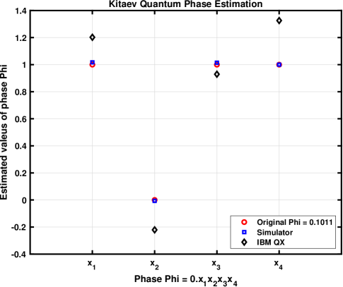
First, we implemented Kitaev algorithm to find the phase $\phi$ on both IBM Qasm Simulator and IBMQ 20-qubit Tokyo quantum computer. We set the $phi=0.x_{1}x_{2}x_{3}x_{4}$ with the value of $0.1011$ and run $1,000$ shots for both simulator and experiment. Fig. 6 shows that the estimated $phi$ values of simulator results are almost the same as the original $phi$ values. The estimated $phi$ values from IBM QX experiment results are slightly different than the original $phi$ due to the lack of full error correction capability of quantum computers yet. However, we can estimate the correct binary values of digits by converting the estimated $phi$ values. Since the noise can be various among different quantum computers, it is critical to find the hardware error rates in order to increase the accuracy of the $phi$ estimation in Kitaev algorithm.

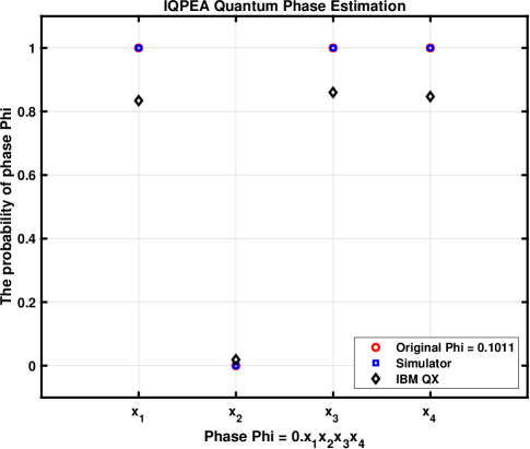
Second, we implemented iterrative quantum phase estimation algorithm (IQPEA) to find the phase $\phi$ on both IBM Qasm Simulator and IBMQ 20-qubit Tokyo quantum computer. Fig. 7 shows that the probability of finding $phi$ value for the simulation results are exactly the same as the original $phi$. IBM QX experiment results are slightly different than the original $phi$ due to the lack of full error correction capability of quantum computers yet. However, we can estimate the correct binary values of digits by converting the estimated $phi$ values. Since the noise can be various among different quantum computers, it is critical to find the hardware error rates in order to increase the accuracy of the $phi$ estimation in IQPEA algorithm.

Figure 8: Lloyd Quantum Phase Estimation Algorithm Gate with 4 qubits and 1 ancillary control qubit

Figure 9: Lloyd Quantum Phase Estimation Algorithm on IBM Tokyo QX 4 qubits

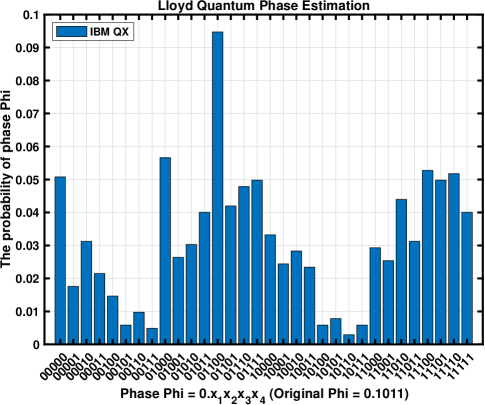
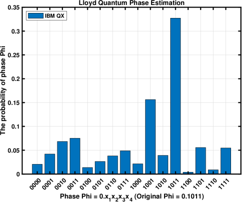
Last, we implemented Lloyd algorithm to find the phase $\phi$ on both IBM Qasm Simulator and IBMQ 20-qubit Tokyo quantum computer. We set the same $phi=0.x_{1}x_{2}x_{3}x_{4}$ value as Kitaev algorithm. Fig. 11 only shows the probability of finding $phi$ values from IBM QX experiment results because the probability of finding $phi$ value for the simulation results are exactly the same as the original $phi$. However, the probability of finding the correct $phi$ from IBM QX results is 0.521 $\%$

Figure 10: Lloyd Quantum Phase Estimation Algorithm Gate

Figure 11: Advanced Lloyd Quantum Phase Estimation Algorithm on IBM Tokyo QX

VII CONCLUSIONS

In this paper

References

- [1] C. P. Williams, Explorations in Quantum Computing. Springer London, 2011.
- [2] A. Aspuru-Guzik, A. D. Dutoi, P. J. Love, and M. Head- Gordon, Science 309, 1704 (2005).
- [3] B. P. Lanyon et al., “Towards quantum chemistry on a quantum computer,” Nature Chemistry, vol. 2, no. 2, pp. 106–111, Jan. 2010.
- [4] P. W. Shor, “Polynomial-Time Algorithms for Prime Factorization and Discrete Logarithms on a Quantum Computer,” SIAM Journal on Computing, vol. 26, no. 5, pp. 1484–1509, Oct. 1997.
- [5] K. Temme, T. J. Osborne, K. G. Vollbrecht, D. Poulin, and F. Verstraete, “Quantum Metropolis sampling,” Nature, vol. 471, no. 7336, pp. 87–90, Mar. 2011.
- [6] M. Ozols, M. Roetteler, and J. Roland, “Quantum rejection sampling,” in Proceedings of the 3rd Innovations in Theoretical Computer Science Conference on - ITCS ’12, 2012.
- [7] L. M. K. Vandersypen, M. Steffen, G. Breyta, C. S. Yannoni, M. H. Sherwood, and I. L. Chuang, “Experimental realization of Shor’s quantum factoring algorithm using nuclear magnetic resonance,” Nature, vol. 414, no. 6866, pp. 883–887, Dec. 2001.
- [8] A. Politi, J. C. F. Matthews, and J. L. O’Brien, “Shor’s Quantum Factoring Algorithm on a Photonic Chip,” Science, vol. 325, no. 5945, pp. 1221–1221, Sep. 2009.
- [9] L. M. K. Vandersypen, M. Steffen, G. Breyta, C. S. Yannoni, M. H. Sherwood, and I. L. Chuang, “Experimental realization of Shor’s quantum factoring algorithm using nuclear magnetic resonance,” Nature, vol. 414, no. 6866, pp. 883–887, Dec. 2001.
- [10] X. Peng et al., “Quantum Adiabatic Algorithm for Factorization and Its Experimental Implementation,” Physical Review Letters, vol. 101, no. 22, Nov. 2008.
- [11] N. Xu, J. Zhu, D. Lu, X. Zhou, X. Peng, and J. Du, “Quantum Factorization of 143 on a Dipolar-Coupling Nuclear Magnetic Resonance System,” Physical Review Letters, vol. 108, no. 13, Mar. 2012.
- [12] A. Y. Kitaev, “Quantum computations: algorithms and error correction,” Russian Mathematical Surveys, vol. 52, no. 6, pp. 1191–1249, Dec. 1997.
- [13] A. Y. Kitaev, A. Shen, and M. Vyalyi, Classical and Quantum Computation (American Mathematical Society, Providence, Rhode Island, 2002).
- [14] D. S. Abrams and S. Lloyd, “Quantum Algorithm Providing Exponential Speed Increase for Finding Eigenvalues and Eigenvectors,” Physical Review Letters, vol. 83, no. 24, pp. 5162–5165, Dec. 1999.
- [15] B. T. Torosov and N. V. Vitanov, “Design of quantum Fourier transforms and quantum algorithms by using circulant Hamiltonians,” Physical Review A, vol. 80, no. 2, Aug. 2009.
- [16] J S. Lee, J. Kim, Y. Cheong, and S. Lee, “Implementation of phase estimation and quantum counting algorithms on an NMR quantum-information processor,” Physical Review A, vol. 66, no. 4, Oct. 2002.
- [17] C. Travaglione and G. J. Milburn, “Generation of eigenstates using the phase-estimation algorithm,” Physical Review A, vol. 63, no. 3, Feb. 2001.
- [18] R. Cleve, A. Ekert, C. Macchiavello, and M. Mosca, “Quantum algorithms revisited,” Proceedings of the Royal Society of London. Series A: Mathematical, Physical and Engineering Sciences, vol. 454, no. 1969, pp. 339–354, Jan. 1998.
- [19] S. Lloyd, M. Mohseni, and P. Rebentrost, “Quantum principal component analysis,” Nature Physics, vol. 10, no. 9, pp. 631–633, Jul. 2014.
- [20] Rebentrost,Patrick and Mohseni, Masoud and Lloyd, Seth “Quantum Support Vector Machine for Big Data Classification” Phys. Rev. Lett., vol. 113, pp. 130503, sep. 2014.
- [21] M. A. Nielsen and I. L. Chuang, Quantum Computation and Quantum Information (Cambridge University Press, Cambridge, 2000).