A family of entire functions connecting the Bessel function $J_{1}$ and the Lambert $W$ function

Abstract

Motivated by the problem of determining the values of $\alpha>0$ for which $f_{\alpha}(x)=e^{\alpha}-(1+1/x)^{\alpha x},\ x>0$ is a completely monotonic function, we combine Fourier analysis with complex analysis to find a family $\varphi_{\alpha}$, $\alpha>0$, of entire functions such that $f_{\alpha}(x)=\int_{0}^{\infty}e^{-sx}\varphi_{\alpha}(s)\,ds,\ x>0.$

We show that each function $\varphi_{\alpha}$ has an expansion in power series, whose coefficients are determined in terms of Bell polynomials. This expansion leads to several properties of the functions $\varphi_{\alpha}$, which turn out to be related to the well known Bessel function $J_{1}$ and the Lambert $W$ function.

On the other hand, by numerically evaluating the series expansion, we are able to show the behavior of $\varphi_{\alpha}$ as $\alpha$ increases from $0$ to $\infty$ and to obtain a very precise approximation of the largest $\alpha>0$ such that $\varphi_{\alpha}(s)\geq 0,\,s>0$, or equivalently, such that $f_{\alpha}$ is completely monotonic.

AMS Subject Classification: 26A48, 30E20, 42A38, 33F05.
Keywords: completely monotonic function, complex analysis, Fourier analysis, Stieltjes moment sequence, Bell polynomials.

1 Introduction and main results

A completely monotonic function is an infinitely differentiable function $f:\left]0,\infty\right[\to\mathbb{R}$ such that

$$(-1)^{n}f^{(n)}(x)\geq 0,\quad x>0,\;n=0,1,\ldots,$$

and a Bernstein function is an infinitely differentiable function $f:\left]0,\infty\right[\to\mathbb{R}$ such that $f(x)\geq 0$ for $x>0$ and $f^{\prime}$ is completely monotonic. Both classes of functions are treated in [4] and [13]. The only completely monotonic functions, which are also Bernstein functions, are the non-negative constant functions.

Let $\alpha>0,\beta\in\mathbb{R}$. In [1, p. 457] it was proved that $(1+\alpha/x)^{x+\beta}-e^{\alpha}$ is completely monotonic if and only if $\alpha\leq 2\beta$. This was sharpened in [10] to a proof that $(1+\alpha/x)^{x+\beta}$ is logarithmically completely monotonic if and only if $\alpha\leq 2\beta$. Monotonicity properties of $(1+\alpha/x)^{x+\beta}$ when $\alpha<0$ has been examined in [9] and [8].

For $\alpha>0$ define

$$f_{\alpha}(x)=e^{\alpha}-h_{\alpha}(x),\quad h_{\alpha}(x)=(1+1/x)^{\alpha x},\quad x>0.$$

In [1, p. 458] it was left as an open problem to determine the values of $\alpha>0$ for which $e^{\alpha}-(1+\alpha/x)^{x}$ is completely monotonic or equivalently $f_{\alpha}$ is completely monotonic. It was proved that $f_{\alpha}$ is completely monotonic for $0<\alpha\leq 1$, and the question was, if $f_{\alpha}$ is completely monotonic for some $\alpha>1$. In [2] the problem was given the equivalent formulation of determining the set of values $\alpha>0$ such that $h_{\alpha}$ is a Bernstein function. It was noticed in [2] that $h_{1}$ is a Bernstein function, because $f_{1}$ is completely monotonic, but $h_{3}$ is not a Bernstein function. Because of the fact that if $f$ is a Bernstein function, then so is $f^{c}$ for $0<c<1$, and the fact that the set of Bernstein functions is closed under pointwise convergence, the set in question is of the form $]0,\alpha^{*}]$, where $\alpha^{*}$ is an unknown number in the interval $[1,3[$. From graphs it looked probable that $\alpha^{*}>2$.

In [14] it was established numerically that $\alpha^{*}\approx 2.29965\,6443.$ This was done looking at monotonicity properties of high order derivatives of $f_{\alpha}$. More precisely, defining

$$f(x,\alpha,n):=(-1)^{n}f_{\alpha}^{(n)}(x),\quad n=0,1,\ldots$$

and letting $\alpha_{n},x_{n}$ be determined as the ”smallest positive solutions” to

$$f(x_{n},\alpha_{n},n+1)=f(x_{n},\alpha_{n},n+2)=0,$$

then $\alpha_{n}$ decreases to $\alpha^{*}$. The estimate for $\alpha^{*}$ is then obtained from approximate values of $\alpha_{n}$ for certain $n$ up to $n=10^{5}$.

In this paper we shall combine Fourier analysis with complex analysis to find a family of entire functions $\varphi_{\alpha},\alpha>0$ such that

$$f_{\alpha}(x)=\int_{0}^{\infty}e^{-sx}\varphi_{\alpha}(s)\,ds,\quad x>0.$$ (1)

By a theorem of Bernstein, cf. [15, p.160], this formula shows that $f_{\alpha}$ is completely monotonic if and only if $\varphi_{\alpha}(s)\geq 0$ for all $s>0$ and therefore $\alpha^{*}$ is determined as the largest $\alpha>0$ such that $\varphi_{\alpha}(s)\geq 0$ for all $s>0$.

It turns out that our calculations leading to (1) are valid for all complex $\alpha$, and for such $\alpha$ we define

$$f_{\alpha}(z)=e^{\alpha}-h_{\alpha}(z),\;$$

$$h_{\alpha}(z)=(1+1/z)^{\alpha z}:=\exp(\alpha z\operatorname{Log}(1+1/z)),\quad z\in\mathcal{A},$$ (2)

where $\mathcal{A}:=\mathbb{C}\setminus]-\infty,0]$ denotes the cut plane, and $\operatorname{Log}$ is the principal logarithm defined in $\mathcal{A}$.

The functions $\varphi_{\alpha}$ are given as contour integrals in the following theorem:

Theorem 1.1.

Let $c>1,r>0$ be fixed, and let $C(r,c)$ denote the rectangle with corners $-c\pm ir,\pm ir$ considered as a closed contour with positive orientation. Then for $\alpha\in\mathbb{C}$

$$\varphi_{\alpha}(s):=\frac{1}{2\pi i}\int_{C(r,c)}f_{\alpha}(z)e^{sz}\,dz,\quad s\in\mathbb{C}$$ (3)

is an entire function, which is independent of $c>1,r>0$, and (1) holds for all $\alpha\in\mathbb{C}$. Moreover $\varphi_{\alpha}(s)$ is bounded for $s\in[0,\infty[$ and tends to 0 for $s\to\infty$.

Theorem 1.1 is contained in Theorem 2.6 and in Theorem 2.10. In particular, the formula (1) is proved in Theorem 2.10.

The power series of the entire functions $\varphi_{\alpha}$ are given in the following theorem, depending on a remarkable sequence of polynomials:

Theorem 1.2.

Let $(p_{n})_{n\geq 0}$ denote the sequence of polynomials defined by

$$p_{0}(\alpha)=1,\quad p_{1}(\alpha)=\frac{\alpha}{2},\quad p_{2}(\alpha)=\frac{\alpha}{3}+\frac{\alpha^{2}}{8},\ldots,$$ (4)

and in general

$$p_{n+1}(\alpha)=\frac{\alpha}{n+1}\sum_{k=0}^{n}\frac{k+1}{k+2}p_{n-k}(\alpha),\quad n\geq 0.$$ (5)

For $\alpha\in\mathbb{C}$

$$\varphi_{\alpha}(s)=e^{\alpha}\sum_{n=0}^{\infty}(-1)^{n}p_{n+1}(\alpha)\frac{s^{n}}{n!},\quad s\in\mathbb{C}.$$ (6)

In particular

$$\varphi_{\alpha}(0)=e^{\alpha}\alpha/2.$$ (7)

Some properties of the polynomials $p_{n}$ are given in Proposition 2.8, while Theorem 1.2 is proved in Section 2.

It follows from (6) that $(\alpha,s)\to\varphi_{\alpha}(s)$ is an entire function on $\mathbb{C}^{2}$, and $s\mapsto\varphi_{\alpha}(s)$ is not identically zero when $\alpha\neq 0$, so it has at most countably many zeros $s\in\mathbb{C}$ which are all isolated. Furthermore when $\alpha>0$ then $\varphi_{\alpha}(s)>0$ for $s\leq 0$.

More results that can be deduced from (6) are contained in the following.

Theorem 1.3.

Consider the entire function $\mathbb{C}^{2}\to\mathbb{C}:(\alpha,s)\mapsto\varphi_{\alpha}(s)$.

• $$\lim_{\alpha\to 0}\frac{\varphi_{\alpha}(s)}{\alpha e^{\alpha}}=\sum_{n=0}^{\infty}\frac{(-1)^{n}}{n+2}\frac{s^{n}}{n!}=\left\{\begin{array}[]{ll}\displaystyle\frac{1-(1+s)e^{-s}}{s^{2}},&\mbox{when}\ s\neq 0,\\ \displaystyle\frac{1}{2},&\mbox{when}\ s=0,\end{array}\right.$$

  uniformly for $s$ in compact subsets of the complex plane.

  The limit function has no real zeros but infinitely many complex zeros $s=\xi_{k}=-W(k,-1/e)-1,k\in\mathbb{Z}\setminus\{-1,0\}$, where W(k,z) is the $k$’th branch of the Lambert $W$ function, see [7]. We have

  $$\xi_{1}=\overline{\xi_{-2}}\approx 2.08884-7.46148i,\qquad\xi_{2}=\overline{\xi_{-3}}\approx 2.66406-13.87905i.$$

• Given $n\in\mathbb{N}$, $\varphi_{\alpha}$ has at least $n$ non-real zeros, when $|\alpha|$ is sufficiently small.

• $$\lim_{|\alpha|\to\infty}\frac{{\varphi}_{\alpha}(s/\alpha)}{\alpha\,e^{\alpha}}=\frac{J_{1}(\sqrt{2s})}{\sqrt{2s}}$$

  uniformly for $s$ in compact subsets of the complex plane, where $J_{1}$ is the Bessel function of order 1.

• Given $n\in\mathbb{N}$, $\varphi_{\alpha}$ has at least $n$ simple zeros $s_{1}(\alpha),s_{2}(\alpha),\ldots,s_{n}(\alpha)$ such that $0<|s_{1}(\alpha)|<|s_{2}(\alpha)|<\ldots<|s_{n}(\alpha)|$ for $|\alpha|$ sufficiently large, and they satisfy

  $$\lim_{|\alpha|\to\infty}\alpha s_{k}(\alpha)=\frac{j_{k}^{2}}{2}\qquad\mbox{for all}\;k\leq n,$$

  where $0<j_{1}<j_{2}<\ldots$ are the positive zeros of $J_{1}$.

  If in addition $\alpha>0$, then $s_{j}(\alpha)>0,\ j=1,\ldots,n$.

• For $\alpha>0$, the entire functions $\varphi_{\alpha}$ are of order one and type one.

Remark 1.4.

It is worth observing that Property $(iv)$ above is an analytical proof of the existence of $\alpha^{*}$, in contrast with [2], where this was obtained by computing $f_{3}^{(4)}(0.4)<0$, which implies that $f_{3}$ cannot be completely monotonic.

The proof of Theorem 1.3 is given in Section 6.

If $(p_{n+1}(\alpha))_{n\geq 0}$ is a Stieltjes moment sequence, i.e., if there exists a positive measure $\sigma_{\alpha}$ on $[0,\infty[$ such that

$$p_{n+1}(\alpha)=\int_{0}^{\infty}x^{n}\,d\sigma_{\alpha}(x),\quad n\geq 0,$$ (8)

then it is easy to see that

$$\varphi_{\alpha}(s)=e^{\alpha}\int_{0}^{\infty}e^{-sx}\,d\sigma_{\alpha}(x),\quad s\in\mathbb{C},$$ (9)

and in particular $\varphi_{\alpha}(s)\geq 0$ for $s\geq 0$ and hence $0\leq\alpha\leq\alpha^{*}$.

However, this argument is only useful for $\alpha\leq 1$, in fact, the following holds.

Theorem 1.5.

The following conditions are equivalent:

• $(p_{n+1}(\alpha))_{n\geq 0}$ is a Stieltjes moment sequence.

• $\varphi_{\alpha}$ is completely monotonic.

• $0\leq\alpha\leq 1$.

If the equivalent conditions hold, then $\sigma_{\alpha}$ from (8) is supported by $[0,1]$, and $(p_{n+1}(\alpha))_{n\geq 0}$ is a Hausdorff moment sequence.

The proof is given in Section 3, where we also find the measures $\sigma_{\alpha}$ for $0\leq\alpha\leq 1$ (see the Equations (28) and (35)).

For $\alpha>1$, on the other hand, we show in Theorem 4.1 that the function $\varphi_{\alpha}$ can be decomposed as the sum of a completely monotonic function and a suitable contour integral (see Equation (40)).

Even so, we have not been able to find an expression which turns out useful in order to check if $\varphi_{\alpha}$ is non-negative on $[0,\infty[$. As a consequence, for these values of $\alpha$, we have to rely on numerical calculation. For this purpose one can use the contour integral (3), but we prefer to use the power series (6), because of the following result.

Theorem 1.6.

For $\alpha>0$, $n\geq 0$, we know that $p_{n}(\alpha)>0$ and

$$\frac{p_{n+1}(\alpha)}{p_{n}(\alpha)}\leq\widehat{\alpha}:=\left\{\begin{array}[]{lll}1,&\mbox{when}\,0\leq\alpha\leq 1,\\ 2\alpha,&\mbox{when}\,1<\alpha<2,\\ \alpha,&\mbox{when}\,2\leq\alpha.\end{array}\right.$$ (10)

Then the series (6) satisfies the Alternating Series Test for $n\geq\widehat{\alpha}s$, which allows to obtain an error bound for the truncated series.

The proof of Theorem 1.6 is given in Section 5.

We summarize what can be seen from the numerical calculations in the following.

Theorem 1.7 (Numerical results).

• $\alpha^{*}\approx 2.29965\,64432\,53461\,30332$.

• For $0<\alpha<\alpha^{*}$ we have $\varphi_{\alpha}(s)>0$ for $s\geq 0$.

• $\varphi_{\alpha^{*}}(s)\geq 0$ for $s\geq 0$ and it has a unique zero of multiplicity two at $s^{*}\approx 5.27004\,87522\,76132\,37103$.

• For $\alpha^{*}<\alpha$, $\varphi_{\alpha}$ has a finite number of positive zeros $0<s_{1}(\alpha)<s_{2}(\alpha)<\ldots<s_{n}(\alpha)$ which are all simple with the exception that the last can be double.

• $s_{1}(\alpha)$ is a simple zero with $\varphi_{\alpha}^{\prime}(s_{1}(\alpha))<0$, moreover $s_{1}(\alpha)$ is a decreasing function on $]\alpha^{*},\infty[$.

Below we present several graphs that support the claims in Theorem 1.7.

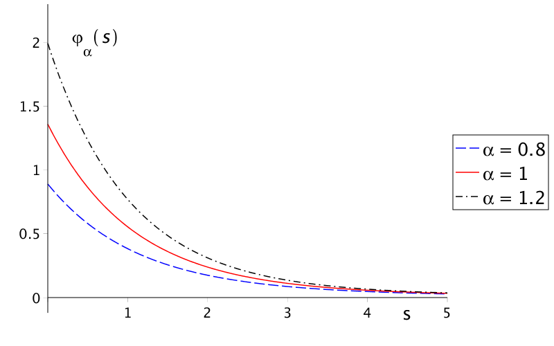
Figure 1: $\varphi_{\alpha}$ near $\alpha=1$

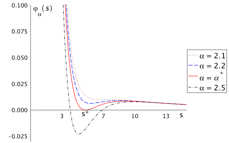
Figure 2: $\varphi_{\alpha}$ below, at, and above $\alpha^{*}$

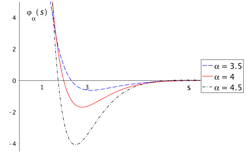
Figure 3: $s_{1}(\alpha)$ decreases

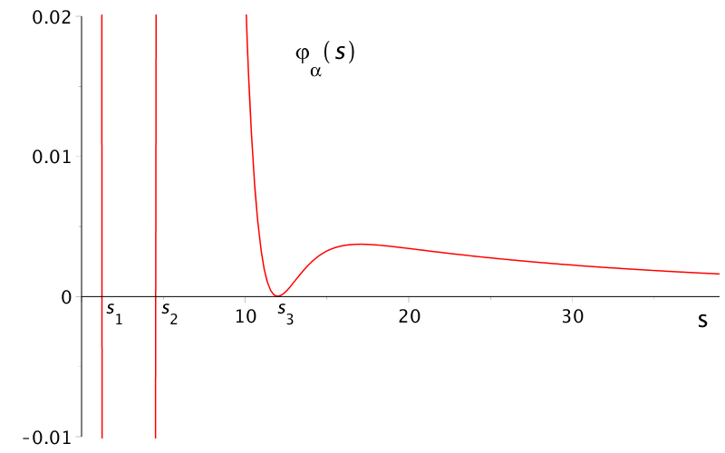
Figure 4: Formation of a third zero ($\alpha\approx 5.988$)

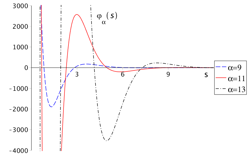
Figure 5: Increasing oscillations at larger $\alpha$

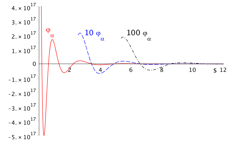
Figure 6: Oscillations at $\alpha=40$

In Figure 1 the graph of ${\varphi}_{\alpha}$ is sketched for the values $\alpha=0.8,\ 1,\ 1.2$: in these cases ${\varphi}_{\alpha}$ is strictly positive (see Property $(ii)$) and, for $\alpha=0.8,\ 1$, also completely monotonic, as stated in Theorem 1.5.

In Figure 2 one can see the graph of ${\varphi}_{\alpha}$ for the value $\alpha=\alpha^{*}$ given in $(i)$, where it presents a unique zero $s^{*}$, which is also a global minimum, as described in $(iii)$. On the other hand, ${\varphi}_{\alpha}$ is still strictly positive for $\alpha<\alpha^{*}$ and has a region of negative values between two simple zeros for $\alpha>\alpha^{*}$.

As $\alpha$ increases, the first zero $s_{1}(\alpha)$ decreases as described in $(v)$ (Figure 3). For $\alpha\approx 5.988$ (Figure 4) a new double zero appears on the right of $s_{1}$ and $s_{2}$, and then more and more oscillations appear by the same mechanism (Figure 5). In Figure 6, for instance, $\varphi_{40}$ is represented with 3 different scales, and one can see at least 10 zeros.

The graphs are obtained in Maple by truncating the series (6), taking into consideration Theorem 1.6. The approximated values of $\alpha^{*},\,s^{*}$ given in Theorem 1.7-$(i,\,iii)$ are also obtained from the truncated series by seeking the minimal value $\alpha^{*}$ for which $\varphi_{\alpha^{*}}$ is zero at some $s^{*}>0$. The approximation for $s^{*}$ is then improved using the fact that $\varphi_{\alpha^{*}}^{\prime}(s^{*})=0$.

2 The family $\varphi_{\alpha},\alpha\in\mathbb{C}$ and the polynomials $p_{n}(\alpha)$

From (2) it is easy to see that

$$\lim_{z\in\mathcal{A},z\to 0}f_{\alpha}(z)=e^{\alpha}-1.$$ (11)

Moreover, $h_{0}(x)=1$ for all $x>0$, so $h_{0}$ is both completely monotonic and a Bernstein function, while $h_{-\alpha}(x)$ is completely monotonic for all $\alpha>0$ because of [4, Proposition 9.2], where we use that

$$x\log(1+1/x)=\int_{0}^{1}\left(1-\frac{u}{u+x}\right)\,du,\quad x>0$$

is a Bernstein function. In particular $h_{\alpha}$ is not a Bernstein function when $\alpha<0$. This means that the set of $\alpha\in\mathbb{R}$ such that $h_{\alpha}$ is a Bernstein function is the closed interval $[0,\alpha^{*}]$.

For an open set $G\subseteq\mathbb{C}$ we denote by $\mathcal{H}(G)$ the set of holomorphic functions defined in $G$.

Clearly $f_{\alpha}\in\mathcal{H}(\mathcal{A})$, but we shall see that $f_{\alpha}$ extends to a holomorphic function in $\mathbb{C}\setminus[-1,0]$. In fact, for $z\neq 0,|z|<1$ we have

$$g_{\alpha}(z):=e^{\alpha}-\exp(\alpha z^{-1}\operatorname{Log}(1+z))=e^{\alpha}-\exp(\alpha(1-z/2+z^{2}/3-\cdots)),$$ (12)

so defining $g_{\alpha}(0)=0$, we see that $g_{\alpha}\in\mathcal{H}(\mathbb{D})$, where

$$\mathbb{D}:=\{z\in\mathbb{C}:|z|<1\}.$$

Now $f_{\alpha}(z):=g_{\alpha}(1/z)$ for $|z|>1$ yields a holomorphic extension of $f_{\alpha}$ to $\mathbb{C}\setminus[-1,0]$.

In the next two results we obtain suitable power series expansions for $g_{\alpha}$, $f_{\alpha}$ and $h_{\alpha}$.

Proposition 2.1.

The power series of $g_{\alpha}\in\mathcal{H}(\mathbb{D})$ given by (12) can be written

$$g_{\alpha}(z)=e^{\alpha}\sum_{n=1}^{\infty}(-1)^{n-1}p_{n}(\alpha)z^{n},$$

where $(p_{n}(\alpha))_{n\geq 0}$ is the sequence of polynomials defined in (4) and (5).

Proof.

We use the formula

$$\exp\left(\sum_{k=1}^{\infty}\frac{a_{k}}{k!}z^{k}\right)=\sum_{n=0}^{\infty}\frac{B_{n}(a_{1},\ldots,a_{n})}{n!}z^{n},$$

where $B_{n}$ are the exponential Bell partition polynomials, cf. [6, Section 11.2]. It is known that

$$B_{0}=1,\quad B_{1}(a_{1})=a_{1},\quad B_{2}(a_{1},a_{2})=a_{1}^{2}+a_{2},$$

and in general we have the recursion formula

$$B_{n+1}(a_{1},\ldots,a_{n+1})=\sum_{k=0}^{n}\binom{n}{k}B_{n-k}(a_{1},\ldots,a_{n-k})a_{k+1}.$$

Defining $a_{k}=(-1)^{k}\alpha k!/(k+1),\;k\geq 1$, this gives for $z\in\mathbb{D}$

$$g_{\alpha}(z) = e^{\alpha}-e^{\alpha}\exp\left(\sum_{k=1}^{\infty}(-1)^{k}\alpha\frac{z^{k}}{k+1}\right)$$

$$= -e^{\alpha}\sum_{n=1}^{\infty}\frac{B_{n}(a_{1},\ldots,a_{n})}{n!}z^{n}=e^{\alpha}\sum_{n=1}^{\infty}(-1)^{n-1}p_{n}(\alpha)z^{n},$$

where we have defined

$$p_{n}(\alpha):=(-1)^{n}\frac{B_{n}(a_{1},\ldots,a_{n})}{n!}.$$ (13)

We see by induction that $p_{n}(\alpha)$ is a polynomial in $\alpha$ of degree $n$ such that (4) holds, and the recursion (5) follows like this

$$p_{n+1}(\alpha) = (-1)^{n+1}\frac{B_{n+1}(a_{1},\ldots,a_{n+1})}{(n+1)!}$$

$$= \frac{1}{n+1}\sum_{k=0}^{n}\frac{1}{k!}(-1)^{n-k}\frac{B_{n-k}(a_{1},\ldots,a_{n-k})}{(n-k)!}(-1)^{k+1}a_{k+1}$$

$$= \frac{\alpha}{n+1}\sum_{k=0}^{n}\frac{k+1}{k+2}p_{n-k}(\alpha).$$

∎

Corollary 2.2.

For $|z|>1$ we have the Laurent expansions

$$f_{\alpha}(z)=e^{\alpha}\sum_{n=1}^{\infty}(-1)^{n-1}\frac{p_{n}(\alpha)}{z^{n}},\quad h_{\alpha}(z)=e^{\alpha}\sum_{n=0}^{\infty}(-1)^{n}\frac{p_{n}(\alpha)}{z^{n}}$$ (14)

and in particular

$$f_{\alpha}(z)=(\alpha/2)e^{\alpha}z^{-1}+\mathcal{O}(|z|^{-2}),\quad|z|>1,|z|\to\infty.$$ (15)

In the following lemma we study the restriction of the function $f_{\alpha}$ to the imaginary axis.

Lemma 2.3.

Let $\alpha\in\mathbb{C}\setminus\{0\}$. As a function of $y\in\mathbb{R}$

$$F_{\alpha}(y):=\left\{\begin{array}[]{lll}f_{\alpha}(iy)=e^{\alpha}-\left(1+y^{-2}\right)^{i\alpha y/2}\exp(\alpha y\operatorname{Arctan}(1/y)),&y\neq 0,\\ e^{\alpha}-1,&y=0,\end{array}\right.$$

is continuous and tends to 0 for $|y|\to\infty$. It belongs to $L^{2}(\mathbb{R})\setminus L^{1}(\mathbb{R})$.

Proof.

We have for $y\neq 0$

$$\exp(i\alpha y\operatorname{Log}(1-i/y))=\exp(i\alpha y[\log\sqrt{1+y^{-2}}-i\operatorname{Arctan}(1/y)]),$$

where $\operatorname{Arctan}:\mathbb{R}\to]-\pi/2,\pi/2[$ is the inverse of $\tan$. The continuity of $F_{\alpha}$ for $y=0$ follows, and the behavior at $\pm\infty$ including the integrability properties follows from Corollary 2.2. ∎

By Plancherel’s Theorem $F_{\alpha}$ is the Fourier-Plancherel transform of another $L^{2}$-function $G_{\alpha}$:

$$f_{\alpha}(iy)=\lim_{R\to\infty}\int_{-R}^{R}G_{\alpha}(s)e^{-iys}\,ds,\quad y\in\mathbb{R},$$ (16)

where the limit is in $L^{2}(\mathbb{R})$, and by the inversion theorem $G_{\alpha}$ is given as

$$G_{\alpha}(s)=\lim_{R\to\infty}\frac{1}{2\pi}\int_{-R}^{R}f_{\alpha}(iy)e^{iys}\,dy,\quad s\in\mathbb{R},$$ (17)

where again the limit is in $L^{2}(\mathbb{R})$. For certain sequences $R_{n}\to\infty$ we also know that

$$\lim_{n\to\infty}\frac{1}{2\pi}\int_{-R_{n}}^{R_{n}}f_{\alpha}(iy)e^{iys}\,dy=G_{\alpha}(s)$$ (18)

for almost all $s\in\mathbb{R}$. Furthermore,

$$\frac{1}{2\pi}\int_{-\infty}^{\infty}|f_{\alpha}(iy)|^{2}\,dy=\int_{-\infty}^{\infty}|G_{\alpha}(s)|^{2}\,ds.$$ (19)

Remark 2.4.

The above formulas (16)-(19) hold trivially for $\alpha=0$ with $F_{0}=G_{0}=0$.

Lemma 2.5.

We have $G_{\alpha}(s)=0$ for $s<0$.

Proof.

Let $C_{R}$ denote the half-circle with radius $R$

$$C_{R}=[-iR,iR]\cup\{Re^{it}:-\pi/2\leq t\leq\pi/2\},$$

considered as a positively oriented closed contour.

Since $f_{\alpha}(z)e^{sz}$ is holomorphic in $\operatorname{Re}z>0$ with a continuous extension to the closed right half-plane bounded by the vertical line $i\mathbb{R}$, we have by Cauchy’s integral theorem

$$\int_{-R}^{R}f_{\alpha}(iy)e^{isy}i\,dy=\int_{-\pi/2}^{\pi/2}f_{\alpha}(Re^{it})e^{sRe^{it}}Re^{it}i\,dt.$$

The absolute value of the integrand to the right is by (15) bounded by

$$\frac{C}{R}e^{sR\cos(t)}R$$

for a suitable $C>0$ depending on $\alpha$. If we assume $s<0$, then $sR\cos t\to-\infty$ for $R\to\infty$ when $-\pi/2<t<\pi/2$, so the integral to the right tends to 0 by dominated convergence. Using (18) we now see that $G_{\alpha}(s)=0$ for almost all $s<0$. Since $G_{\alpha}$ is an equivalence class of square integrable functions, we can assume that $G_{\alpha}(s)=0$ for $s<0$. ∎

Exploiting the holomorphy of $f_{\alpha}$ in $\mathbb{C}\setminus[-1,0]$ we can prove part of Theorem 1.1, which is contained in the following.

Theorem 2.6.

For $\alpha\in\mathbb{C}$, the function $\varphi_{\alpha}$ defined in (3) is an entire function, which is independent of $c>1,r>0$.

Moreover, the function

$$s\mapsto\left\{\begin{array}[]{ll}\varphi_{\alpha}(s),&\mbox{when}\ 0\leq s<\infty,\\ 0,&\mbox{when}\,-\infty<s<0,\end{array}\right.$$ (20)

is equal to $G_{\alpha}(s)$ for almost all $s\in\mathbb{R}$.

Remark 2.7.

In the following we denote the function given by (20) as $G_{\alpha}$.

Proof.

It is clear that the function $\varphi_{\alpha}$ from (3) is entire, and also that it is independent of $c>1,r>0$ by Cauchy’s integral theorem.

Let $R>c$ and consider the following three positively oriented closed contours: two quarter circles with radius $R$

$$T_{+}(R) = \{x+ir:x=-R\ldots 0\}$$

$$\cup\;\{iy:y=r\ldots r+R\}\cup\{ir+Re^{i\theta}:\theta=\pi/2\ldots\pi\}$$

$$T_{-}(R) = \{x-ir:x=0\ldots-R\}$$

$$\cup\;\{-ir+Re^{i\theta}:\theta=\pi\ldots 3\pi/2\}\cup\{iy:y=-r-R\ldots-r\}$$

and a rectangle $Q(R)$ with corners $\{-R\pm ir,-c\pm ir\}$. By Cauchy’s integral theorem we have

$$\frac{1}{2\pi i}\int_{T_{\pm}(R)}f_{\alpha}(z)e^{sz}\,dz=\frac{1}{2\pi i}\int_{Q(R)}f_{\alpha}(z)e^{sz}\,dz=0.$$

Adding these three integrals to the contour integral in (3) yields

$$\varphi_{\alpha}(s) = \frac{1}{2\pi i}\int_{C(r,c)}f_{\alpha}(z)e^{sz}\,dz$$

$$= \frac{1}{2\pi i}\int_{-i(r+R)}^{i(r+R)}f_{\alpha}(z)e^{sz}\,dz+\frac{1}{2\pi i}\int_{L(R)}f_{\alpha}(z)e^{sz}\,dz,$$

where $L(R)$ is the following contour

$$\{ir+Re^{i\theta}:\theta=\pi/2\ldots\pi\}\cup\{-R+iy:y=r\ldots-r\}\cup\{-ir+Re^{i\theta}:\theta=\pi\ldots 3\pi/2\}.$$

For $s>0$ we have

$$\lim_{R\to\infty}\frac{1}{2\pi i}\int_{L(R)}f_{\alpha}(z)e^{sz}\,dz=0.$$

In fact, for $z\in L(R)$ we have $|z|\geq R$, hence $|f_{\alpha}(z)|\leq C/R$ for suitable $C>0$ by (15). This gives

$$\left|\frac{1}{2\pi i}\int_{L(R)}f_{\alpha}(z)e^{sz}\,dz\right|\leq\frac{C}{2\pi R}\left[2re^{-sR}+R\int_{\pi/2}^{3\pi/2}e^{sR\cos\theta}\,d\theta\right],$$

which tends to 0 for $R\to\infty$ because $\cos\theta<0$ for $\pi/2<\theta<3\pi/2$. The function

$$I(R)(s):=\frac{1}{2\pi i}\int_{-i(r+R)}^{i(r+R)}f_{\alpha}(z)e^{sz}\,dz$$

converges to $G_{\alpha}(s)$ in $L^{2}(\mathbb{R})$ for $R\to\infty$ by (17), so for a suitable sequence $R_{n}\to\infty$ we know that $I(R_{n})(s)$ converges to $G_{\alpha}(s)$ for almost all $s\in\mathbb{R}$. It follows that $\varphi_{\alpha}(s)=G_{\alpha}(s)$ for almost all $s>0$. Since apriori we only know that $G_{\alpha}$ is an equivalence class of square integrable functions, we can use formula (20) as a representative of $G_{\alpha}$. ∎

At this point we are able to prove Theorem 1.2, that is, to obtain the power series expansion of $\varphi_{\alpha}$.

Proof of Theorem 1.2.

From (3) and the compactness of the contour $C(r,c)$ we get

$$\varphi_{\alpha}(s)=\sum_{n=0}^{\infty}\frac{s^{n}}{n!}\frac{1}{2\pi i}\int_{C(r,c)}f_{\alpha}(z)z^{n}\,dz.$$

Using that $f_{\alpha}(z)z^{n}$ is holomorphic outside $[-1,0]$, we can replace the contour $C(r,c)$ by the circle $|z|=R_{0}$, where $R_{0}>\sqrt{c^{2}+r^{2}}>1$. We next use the Laurent expansion (14) and get

$$\frac{1}{2\pi i}\int_{C(r,c)}f_{\alpha}(z)z^{n}\,dz = \sum_{k=1}^{\infty}e^{\alpha}(-1)^{k-1}p_{k}(\alpha)\frac{1}{2\pi i}\int_{|z|=R_{0}}z^{n-k}\,dz$$

$$= e^{\alpha}(-1)^{n}p_{n+1}(\alpha),$$

which shows (6). ∎

In the following proposition we list several properties of the polynomials $p_{n}$ that appear in the series (6). We prove below the Properties $(i)$ through $(iv)$, in particular, Properties $(i)$ through $(iii)$ will be needed in Theorem 2.10, in order to conclude the proof of Theorem 1.1. The remaining properties rely partially on the results of Section 3 and will be proved in Section 5. See also Remark 7.1 and Equation (55) in the Appendix, for an alternative expression for the polynomials $p_{n}$, based on Stirling numbers.

Proposition 2.8.

The polynomials $p_{n}$ from Theorem 1.2 satisfy Theorem 1.6 and

• $\displaystyle p_{n}(\alpha)=\sum_{k=1}^{n}c_{n,k}\alpha^{k},\quad n\geq 1$, where $c_{n,k}>0$ and
           $\displaystyle c_{n,1}=\frac{1}{(n+1)},\;c_{n,n}=\frac{1}{2^{n}\,n!}\,.$

• $|p_{n}(\alpha)|\leq p_{n}(|\alpha|),\quad\alpha\in\mathbb{C}$.

• $0\leq p_{n}(\alpha)\leq\left\{\begin{array}[]{lll}1,&\mbox{when }\,0\leq\alpha\leq 1,\\ \alpha^{n},&\mbox{when }\,1\leq\alpha,\\ n,&\mbox{when }\,0\leq\alpha\leq 2,n\geq 1.\end{array}\right.$

• For $\alpha,\beta\in\mathbb{C}$ and $n\geq 0$ we have the addition formula

  $$p_{n}(\alpha+\beta)=\sum_{k=0}^{n}p_{k}(\alpha)p_{n-k}(\beta).$$

• The sequence $(p_{n}(\alpha))_{n\geq 0}$ is $\left\{\begin{array}[]{lll}\text{strictly decreasing, }&\text{ for $0<\alpha\leq 1$, }\\ \text{increasing, }&\text{ for $2\leq\alpha$. }\end{array}\right.$

• $\displaystyle\lim_{n\to\infty}p_{n}(\alpha)=\left\{\begin{array}[]{ll}0,&\mbox{when }\,0<\alpha<1,\\ e^{-1},&\mbox{when }\,\alpha=1,\\ \infty,&\mbox{when }\,\alpha>1.\end{array}\right.$

• $\displaystyle\lim_{n\to\infty}\frac{p_{n+1}(\alpha)}{p_{n}(\alpha)}=\lim_{n\to\infty}\root n \of{p_{n}(\alpha)}=1,\,\mbox{when}\ \alpha>0$.

Proof of Proposition 2.8: (i) through (iv).

Property $(i)$ follows easily by induction using the recursion (5), while Property $(ii)$ follows because the coefficients of $p_{n}$ are non-negative.

Property $(iii)$ follows by induction, as described below. The two first inequalities hold for $n=0$, and assuming the assertion for $k\leq n$ we get by (5), for $0\leq\alpha\leq 1$

$$p_{n+1}(\alpha)\leq\frac{1}{n+1}\sum_{k=0}^{n}\frac{k+1}{k+2}\leq 1,$$

and for $1\leq\alpha$

$$p_{n+1}(\alpha)\leq\frac{\alpha}{n+1}\sum_{k=0}^{n}\frac{k+1}{k+2}\alpha^{n-k}\leq\alpha^{n+1}.$$

The last inequality holds for $n=1$, and by induction using $p_{0}(\alpha)=1$ and $p_{k}(\alpha)\leq k$ for $1\leq k\leq n$ we find, for $n\geq 1$,

$$p_{n+1}(\alpha)\leq\frac{\alpha}{n+1}\left(1+\sum_{k=0}^{n-1}(n-k)\right)=\frac{\alpha}{n+1}\left[1+\frac{n(n+1)}{2}\right]\leq\frac{2}{n+1}+n\leq n+1.$$

To see $(iv)$ we notice that by (2) we get

$$h_{\alpha+\beta}(z)=h_{\alpha}(z)h_{\beta}(z),\quad z\in\mathcal{A},$$

and by (14)

$$h_{\alpha}(-1/s)=e^{\alpha}\sum_{n=0}^{\infty}p_{n}(\alpha)s^{n},\quad 0<|s|<1.$$

This implies that

$$\sum_{n=0}^{\infty}p_{n}(\alpha+\beta)s^{n}=\sum_{n=0}^{\infty}p_{n}(\alpha)s^{n}\sum_{m=0}^{\infty}p_{m}(\beta)s^{m},\quad 0<|s|<1,$$ (21)

which clearly holds for $s=0$. Multiplying the absolutely convergent power series for $|s|<1$ in (21), we get the addition formula. ∎

By Theorem 1.2 and Proposition 2.8-$(ii,\,iii)$ we obtain the following.

Corollary 2.9.

The entire functions $\varphi_{\alpha}$ satisfy for $s,\alpha\in\mathbb{C}$

$$|\varphi_{\alpha}(s)|\leq\left\{\begin{array}[]{ll}|e^{\alpha}|e^{|s|}\,,&\mbox{when }\,|\alpha|\leq 1\\ |\alpha||e^{\alpha}|e^{|\alpha s|}\,,&\mbox{when }\,1\leq|\alpha|.\end{array}\right.$$

The order and type of $\varphi_{\alpha}$ when $\alpha>0$ are given in Theorem 1.3-$(v)$.

We can finally conclude the proof of Theorem 1.1, as a consequence of the following.

Theorem 2.10.

For any $\alpha\in\mathbb{C}$, $\varphi_{\alpha}(s)$ is bounded for $s\in[0,\infty[$ and tends to 0 for $s\to\infty$. The following formula holds

$$f_{\alpha}(z)=\int_{0}^{\infty}\varphi_{\alpha}(s)e^{-sz}\,ds,\quad\operatorname{Re}{z}>0.$$ (22)

Proof.

Let us write (3) in another way. Introducing

$$I_{1}(r,s):=\frac{1}{2\pi}\int_{-r}^{r}f_{\alpha}(iy)e^{isy}\,dy,\quad I_{3}(r,s):=\frac{1}{2\pi}\int_{-r}^{r}f_{\alpha}(-c+iy)e^{s(-c+iy)}\,dy,$$

and

$$I_{2}(r,s):=\frac{1}{2\pi i}\int_{-c}^{0}f_{\alpha}(x+ir)e^{s(x+ir)}\,dx,\quad I_{4}(r,s):=\frac{1}{2\pi i}\int_{-c}^{0}f_{\alpha}(x-ir)e^{s(x-ir)}\,dx,$$

we have for $s\geq 0$

$$\varphi_{\alpha}(s)=I_{1}(r,s)-I_{3}(r,s)-I_{2}(r,s)+I_{4}(r,s).$$ (23)

We see by Riemann-Lebesgue’s lemma that $\lim_{s\to\infty}I_{1}(r,s)=0$. Furthermore,

$$|I_{3}(r,s)|\leq\frac{r}{\pi}e^{-sc}\max\{|f_{\alpha}(-c+iy)|:|y|\leq r\}$$

and

$$|I_{2}(r,s)|,|I_{4}(r,s)|\leq\frac{1}{2\pi}\max\{|f_{\alpha}(x\pm ir)|:-c\leq x\leq 0\}\int_{-c}^{0}e^{sx}\,dx$$

show that

$$\lim_{s\to\infty}|I_{j}(r,s)|=0,\quad j=2,3,4.$$

By (23) it follows that $\lim_{s\to\infty}\varphi_{\alpha}(s)=0$. This property together with the continuity of $\varphi_{\alpha}$ imply that $\varphi_{\alpha}$ is bounded on $[0,\infty[$.

To prove the formula (22) we note that the right-hand side is holomorphic for $\operatorname{Re}z>0$, and so is the left-hand side.

For $s\geq 0$ we have by Proposition 2.8-$(ii,\,iii)$

$$\left|\sum_{n=0}^{N}(-1)^{n}p_{n+1}(\alpha)\frac{s^{n}}{n!}\right|\leq\sum_{n=0}^{N}p_{n+1}(|\alpha|)\frac{s^{n}}{n!}\leq\left\{\begin{array}[]{ll}e^{s},&\mbox{if}\;|\alpha|\leq 1\\ |\alpha|e^{|\alpha|s},&\mbox{if}\;|\alpha|\geq 1.\end{array}\right.$$ (24)

For $x>0$ we have

$$\int_{0}^{\infty}e^{\alpha}\left(\sum_{n=0}^{N}(-1)^{n}p_{n+1}(\alpha)\frac{s^{n}}{n!}\right)e^{-sx}\,ds$$

$$= e^{\alpha}\sum_{n=0}^{N}(-1)^{n}p_{n+1}(\alpha)\int_{0}^{\infty}\frac{s^{n}}{n!}e^{-sx}\,ds=e^{\alpha}\sum_{n=0}^{N}(-1)^{n}\frac{p_{n+1}(\alpha)}{x^{n+1}}.$$

Assume now $x>\max(1,|\alpha|)$. For $N\to\infty$ the last expression converges to $f_{\alpha}(x)$ by Corollary 2.2. The integrand in the first expression converges for each $s\geq 0$ to $\varphi_{\alpha}(s)e^{-sx}$ with an integrable majorant because of (24), so by Lebesgue’s Theorem on dominated convergence, we get

$$\int_{0}^{\infty}\varphi_{\alpha}(s)e^{-sx}\,ds=f_{\alpha}(x),\quad x>\max(1,|\alpha|).$$

This is enough to conclude (22). ∎

As discussed in the Introduction, we can now state the following important result.

Theorem 2.11.

For $\alpha\in\mathbb{C}$, $f_{\alpha}$ is completely monotonic if and only if $\varphi_{\alpha}(s)\geq 0$ for $s\geq 0$. In the affirmative case $\varphi_{\alpha}$ is integrable on $[0,\infty[$ and

$$\lim_{x\to 0^{+}}f_{\alpha}(x)=e^{\alpha}-1=\int_{0}^{\infty}\varphi_{\alpha}(s)\,ds.$$ (25)

Moreover, in this case (22) holds for $\operatorname{Re}{z}\geq 0$ and

$$h_{\alpha}(z)=1+\int_{0}^{\infty}(1-e^{-sz})\varphi_{\alpha}(s)\,ds,\quad\operatorname{Re}{z}\geq 0,z\neq 0.$$ (26)

Proof.

The first assertion follows from Bernstein’s characterization of completely monotonic functions as Laplace transforms of positive measures. Equation (25) follows from (11), (22) and the monotonicity theorem of Lebesgue.

When $\varphi_{\alpha}$ is integrable over $[0,\infty[$, the right-hand side of (22) is continuous in the half-plane $\operatorname{Re}{z}\geq 0$, and since $f_{\alpha}$ is also continuous there, we see that (22) holds for $\operatorname{Re}{z}\geq 0$. The Equation (26) follows easily from (25). ∎

3 The cases $0<\alpha\leq 1$

As mentioned in Section 1, it was proved in [1] that $f_{\alpha}$ is completely monotonic for $0<\alpha\leq 1$ and equivalently $\varphi_{\alpha}$ is non-negative on $[0,\infty[$ for these values of $\alpha$. We shall use the previous results to give a new proof of this. We recall that a function $f:\left]0,\infty\right[\to\mathbb{R}$ is called a Stieltjes function, if it has the form

$$f(s)=a+\int_{0}^{\infty}\frac{d\mu(t)}{s+t},\quad s>0,$$ (27)

where $a\geq 0$ and $\mu$ is a positive measure on $[0,\infty[$. A Stieltjes function is completely monotonic but the converse is not true. For more information about Stieltjes functions see [4] and [3].

We have the following result.

Theorem 3.1.

The function $f_{\alpha}$ is a Stieltjes function for $0\leq\alpha\leq 1$, but not for $\alpha>1$.

The cases $0<\alpha<1$, $\alpha=1$ and $\alpha>1$ are treated separately in Theorem 3.2, Corollary 3.4 and Proposition 3.5.

Theorem 3.2.

For $0<\alpha<1$ we have

$$\varphi_{\alpha}(s)=\frac{1}{\pi}\int_{0}^{1}(x/(1-x))^{\alpha x}\sin(\alpha\pi x)e^{-sx}\,dx,\quad s\geq 0,$$ (28)

and

$$f_{\alpha}(z)=\frac{1}{\pi}\int_{0}^{1}\frac{(x/(1-x))^{\alpha x}\sin(\alpha\pi x)}{x+z}\,dx,\quad z\in\mathbb{C}\setminus[-1,0].$$ (29)

Proof.

Assume $0<\alpha<1$ and let $c,r$ in the contour from Theorem 2.6 be chosen such that $1<c<2,\alpha c<1$ and $0<r<1$.

Let now $r\to 0$ in (23). The first two terms tend to 0. Using that $\alpha$ is real we can write

$$I_{2}(r,s)-I_{4}(r,s)=\frac{1}{\pi}\int_{-c}^{0}e^{sx}\operatorname{Im}\{f_{\alpha}(x+ir)e^{isr}\}\,dx,$$

and replacing $x$ by $-x$ in this expression, we get

$$\varphi_{\alpha}(s) = -\lim_{r\to 0}\frac{1}{\pi}\int_{0}^{c}e^{-sx}\operatorname{Im}\{f_{\alpha}(-x+ir)e^{isr}\}\,dx$$

$$= \lim_{r\to 0}\frac{1}{\pi}\int_{0}^{c}e^{-sx}\operatorname{Im}\left\{\exp\left[\alpha(-x+ir)\operatorname{Log}\left(1+\frac{1}{-x+ir}\right)+irs\right]\right\}\,dx.$$

We have

$$\operatorname{Log}\left(1+\frac{1}{-x+ir}\right)=K(x,r)-i\theta(x,r)$$

where

$$K(x,r)=\frac{1}{2}\log\frac{(1-x)^{2}+r^{2}}{x^{2}+r^{2}},\quad\cot\theta(x,r)=\frac{x(x-1)+r^{2}}{r}$$

and $\theta(x,r)\in\left]0,\pi\right[$.

We therefore have (leaving out the arguments in $K(x,r),\theta(x,r)$ to simplify notation)

$$J_{r}(x) := \operatorname{Im}\left\{\exp\left[\alpha(-x+ir)\operatorname{Log}\left(1+\frac{1}{-x+ir}\right)+irs\right]\right\}$$

$$= \exp[\alpha(-xK+r\theta)]\sin[\alpha(rK+x\theta)+rs]$$

$$= \left(\frac{x^{2}+r^{2}}{(1-x)^{2}+r^{2}}\right)^{(\alpha x)/2}\exp(\alpha r\theta)\sin[\alpha(rK+x\theta)+rs],$$

and hence

$$\lim_{r\to 0}J_{r}(x)=\left\{\begin{array}[]{lll}(x/(1-x))^{\alpha x}\sin(\alpha\pi x),&\mbox{when}\,0<x<1,\\ \infty,&\mbox{when}\,x=1,\\ 0,&\mbox{when}\,1<x<c.\end{array}\right.$$

We have the following inequalities for $0<x<c$, using that $|x-1|<1$,

$$|J_{r}(x)| \leq \left(\frac{x^{2}+r^{2}}{(1-x)^{2}+r^{2}}\right)^{(\alpha x)/2}\exp(\alpha\pi)\leq\frac{(c^{2}+1)^{(\alpha c)/2}\exp(\alpha\pi)}{|1-x|^{\alpha c}},$$

and since $\alpha c<1$, the last expression is an integrable majorant over $]0,c[$. By Lebesgue’s Theorem we therefore get

$$\varphi_{\alpha}(s)=\frac{1}{\pi}\int_{0}^{1}\left(x/(1-x)\right)^{\alpha x}\sin(\alpha\pi x)e^{-sx}\,dx,$$ (30)

so $\varphi_{\alpha}(s)>0$ for $s\geq 0$ and $0<\alpha<1$.

Inserting (30) in (22) we get

$$f_{\alpha}(z)=\frac{1}{\pi}\int_{0}^{1}\frac{\left(x/(1-x)\right)^{\alpha x}\sin(\alpha\pi x)}{x+z}\,dx,\qquad\text{for $\operatorname{Re}{z}>0$.}$$ (31)

By the identity theorem for holomorphic functions (31) holds for $z\notin[-1,0]$. ∎

Equation (30) shows that $\varphi_{\alpha}$ is completely monotonic for $0<\alpha<1$. For $\alpha\to 1^{-}$ we get that $\varphi_{1}$ is completely monotonic and in particular non-negative, and by [4, Section 14.12] we get that $f_{1}$ is a Stieltjes function.

To find the representations of $\varphi_{1}$ and $f_{1}$ in analogy with (30) and (31), it turns out not to be correct to replace $\alpha$ by 1 in these formulas.

Let us introduce the notation

$$u(\alpha,x)=\left(x/(1-x)\right)^{\alpha x}\sin(\alpha\pi x),\quad 0<\alpha\leq 1,0\leq x<1.$$

Clearly $u(\alpha,x)\geq 0$, and $u(1,x)$ is seen to be bounded by $\pi$, while

$$\lim_{x\to 1}u(\alpha,x)=\infty,\quad 0<\alpha<1.$$

Proposition 3.3.

For $0<\alpha<1$ define

$$w(\alpha,x)=u(\alpha,x)-u(1,x),\quad 0\leq x<1.$$

Then for any $\phi\in C([0,1])$ we have

$$\lim_{\alpha\to 1^{-}}\frac{1}{\pi}\int_{0}^{1}w(\alpha,x)\phi(x)\,dx=\phi(1).$$ (32)

Proof.

We need the following partial results:

Step 1: $\lim_{\alpha\to 1^{-}}w(\alpha,x)=0$ for $0\leq x<1$, uniformly for $x\in[0,1-\delta]$ for any $0<\delta<1$.

This is clear.

Step 2:

$$\lim_{\alpha\to 1^{-}}\frac{1}{\pi}\int_{0}^{1}w(\alpha,x)\,dx=1.$$

To see this, note that by (28) and (7)

$$\frac{1}{\pi}\int_{0}^{1}u(\alpha,x)\,dx=\varphi_{\alpha}(0)=\frac{\alpha}{2}\,e^{\alpha}$$ (33)

and

$$\frac{1}{\pi}\int_{0}^{1}u(1,x)\,dx=\frac{1}{\pi}\int_{0}^{1}\left(x/(1-x)\right)^{x}\sin(\pi x)\,dx=\frac{e}{2}-1,$$ (34)

see [1, Lemma 2, p. 4]. Therefore

$$\frac{1}{\pi}\int_{0}^{1}w(\alpha,x)\,dx=\frac{\alpha}{2}\,e^{\alpha}-\frac{e}{2}+1,$$

which has limit 1 for $\alpha\to 1$, proving Step 2.

Let now $\phi\in C([0,1])$. Let $\varepsilon>0$ be given and by continuity choose $x_{1}<1$ such that $|\phi(x)-\phi(1)|<\varepsilon$ for $x_{1}\leq x\leq 1$. We can then write

$$\frac{1}{\pi}\int_{0}^{1}w(\alpha,x)\phi(x)\,dx-\phi(1)$$

$$= \frac{1}{\pi}\int_{0}^{x_{1}}w(\alpha,x)\phi(x)\,dx+\frac{1}{\pi}\int_{x_{1}}^{1}w(\alpha,x)(\phi(x)-\phi(1))\,dx$$

$$+ \phi(1)\left(\frac{1}{\pi}\int_{x_{1}}^{1}w(\alpha,x)\,dx-1\right):=\sum_{j=1}^{3}T_{j}(\alpha),$$

and hence

$$\left|\frac{1}{\pi}\int_{0}^{1}w(\alpha,x)\phi(x)\,dx-\phi(1)\right|\leq\sum_{j=1}^{3}|T_{j}(\alpha)|.$$

By Step 1 we know that $|T_{1}(\alpha)|\to 0$ for $\alpha\to 1^{-}$. Furthermore, by (33) and (34) we find

$$|T_{2}(\alpha)| \leq \frac{1}{\pi}\int_{x_{1}}^{1}|w(\alpha,x)||\phi(x)-\phi(1)|\,dx\leq\frac{\varepsilon}{\pi}\int_{x_{1}}^{1}|w(\alpha,x)|\,dx$$

$$\leq \frac{\varepsilon}{\pi}\int_{0}^{1}(u(\alpha,x)+u(1,x))\,dx=\varepsilon\left(\frac{\alpha}{2}\,e^{\alpha}+\frac{e}{2}\,-1\right)\leq\varepsilon(e-1).$$

Finally, $|T_{3}(\alpha)|$ tends to 0 for $\alpha\to 1^{-}$ because

$$|T_{3}(\alpha)|=|\phi(1)|\left|\frac{1}{\pi}\int_{0}^{1}w(\alpha,x)\,dx-1-\frac{1}{\pi}\int_{0}^{x_{1}}w(\alpha,x)\,dx\right|,$$

and we then use Step 1 and Step 2.

In total we get

$$\limsup_{\alpha\to 1^{-}}\left|\frac{1}{\pi}\int_{0}^{1}w(\alpha,x)\phi(x)\,dx-\phi(1)\right|\leq\varepsilon(e-1),$$

and (32) follows. ∎

Applying the above result to the continuous functions $\phi(x)=e^{-sx}$ and $\phi(x)=(x+z)^{-1}$ for $z\notin[-1,0]$ we get

Corollary 3.4.

$$\varphi_{1}(s)=e^{-s}+\frac{1}{\pi}\int_{0}^{1}\left(x/(1-x)\right)^{x}\sin(\pi x)e^{-sx}\,dx,\quad s\geq 0.$$ (35)

$$f_{1}(z)=\frac{1}{z+1}+\frac{1}{\pi}\int_{0}^{1}\frac{\left(x/(1-x)\right)^{x}\sin(\pi x)}{x+z}\,dx,\quad z\notin[-1,0].$$

Proposition 3.5.

The function $f_{\alpha}$ is not a Stieltjes function when $\alpha>1.$

Proof.

By (27) a non-constant Stieltjes function $f$ has an extension to a holomorphic function in $\mathcal{A}$ satisfying

$$\operatorname{Im}{f(z)}<0\quad\mbox{for}\quad\operatorname{Im}{z}>0,$$ (36)

because for $z=x+iy,y>0$ we have

$$\operatorname{Im}{f(z)}=-y\int_{0}^{\infty}\frac{d\mu(t)}{|z+t|^{2}}<0.$$

For $\alpha>1$ let $0<x<1$ be chosen such that $1<\alpha x<2$. For $y=r>0$ we have

$$\operatorname{Im}{f_{\alpha}(-x+ir)}=-\operatorname{Im}\left\{\exp\left[\alpha(-x+ir)\operatorname{Log}\left(1+\frac{1}{-x+ir}\right)\right]\right\},$$

and proceeding as in the proof of Theorem 3.2 we get

$$\lim_{r\to 0}\operatorname{Im}{f_{\alpha}(-x+ir)}=-(x/(1-x))^{\alpha x}\sin(\alpha\pi x)>0.$$

This shows that $\operatorname{Im}{f_{\alpha}(-x+ir)}>0$ for $r>0$ sufficiently small. By (36) this shows that $f_{\alpha}$ is not a Stieltjes function when $\alpha>1$. ∎

Using the formulas for $\varphi_{\alpha}$ in Theorem 3.2 and Corollary 3.4 we can prove that the sequence $(p_{n+1}(\alpha))_{n\geq 0}$ is a Hausdorff moment sequence, i.e., the moment sequence of a positive measure on $[0,1]$.

Theorem 3.6.

For $0<\alpha<1$ we have

$$p_{n+1}(\alpha)=\frac{e^{-\alpha}}{\pi}\int_{0}^{1}(x/(1-x))^{\alpha x}\sin(\alpha\pi x)x^{n}\,dx,\quad n\geq 0,$$ (37)

while for $\alpha=1$

$$p_{n+1}(1)=e^{-1}+\frac{e^{-1}}{\pi}\int_{0}^{1}(x/(1-x))^{x}\sin(\pi x)x^{n}\,dx,\quad n\geq 0.$$ (38)

Proof.

Inserting the power series for $e^{-sx}$ in Equation (28) and interchanging summation and integration, we get the power series expansion for $\varphi_{\alpha}$. Compared with (6) this yields (37).

To get the case $\alpha=1$ we can proceed similarly with the formula for $\varphi_{1}$ in Corollary 3.4, or we can apply Proposition 3.3 to $\phi(x)=x^{n}$. ∎

See Remark 7.2 in the Appendix, for a proof that the sequence $(p_{n}(\alpha))_{n\geq 0}$ is also a Hausdorff moment sequence.

We can now prove the equivalence of the three conditions in Theorem 1.5.

Proof of Theorem 1.5.

”$(i)\Rightarrow(ii)$” If $(p_{n+1}(\alpha))_{n\geq 0}$ is a Stieltjes moment sequence, i.e., (8) holds for a positive measure $\sigma_{\alpha}$ on $[0,\infty[$, then $\alpha=2p_{1}(\alpha)=2\int_{0}^{\infty}\,d\sigma_{\alpha}(x)\geq 0$. Without loss of generality we can assume $\alpha>0$. By Proposition 2.8-$(iii)$ we know that $p_{n}(\alpha)\leq l^{n},\;n\geq 0$, where $l=\max(1,\alpha)$, which implies that $\sigma_{\alpha}$ is supported by the interval $[0,l]$. By (6) we then get

$$\varphi_{\alpha}(s)=e^{\alpha}\sum_{n=0}^{\infty}(-1)^{n}\frac{s^{n}}{n!}\int_{0}^{l}x^{n}\,d\sigma_{\alpha}(x)=e^{\alpha}\int_{0}^{l}e^{-sx}\,d\sigma_{\alpha}(x),$$

which shows that $\varphi_{\alpha}$ is completely monotonic.

”$(ii)\Rightarrow(iii)$” If $\varphi_{\alpha}$ is completely monotonic, hence of the form

$$\varphi_{\alpha}(s)=\int_{0}^{\infty}e^{-ts}\,d\mu(t)$$

for a positive measure $\mu$, we get, using (6),

$$(-1)^{n}\varphi_{\alpha}^{(n)}(0)=\int_{0}^{\infty}t^{n}\,d\mu(t)=e^{\alpha}p_{n+1}(\alpha)\geq 0,\quad n\geq 0$$

but this is only possible if $\alpha\geq 0$. Furthermore,

$$f_{\alpha}(x)=\int_{0}^{\infty}e^{-xs}\varphi_{\alpha}(s)\,ds=\int_{0}^{\infty}\frac{d\mu(t)}{x+t},\quad x>0,$$

so $f_{\alpha}$ is a Stieltjes function and hence $\alpha\leq 1$ by Theorem 3.1.

”$(iii)\Rightarrow(i)$” follows from Theorem 3.6. ∎

4 The case $\alpha>1$

In the previous section we were able to express the functions $\varphi_{\alpha}$ with $0\leq\alpha\leq 1$ as in Equation (9), proving that they are nonnegative on $[0,\infty[.$ The purpose of this section is to show that, for $1<\alpha$, we can still find a component in $\varphi_{\alpha}$ analogous to (9), but a correcting term needs to be added, which is given by a contour integral on a suitable circle that goes around the singularity $-1$: see Equations (40) and (41).

For $a\in\mathbb{C}$ and $r>0$ we denote by $\partial D(a,r)$ the positively oriented circle with center $a$ and radius $r$.

Let $\alpha>1$ be fixed, and let $0<\varepsilon<1-1/\alpha$. We consider the closed positively oriented contour $T(\alpha,\varepsilon)$ starting at $i\varepsilon$, then moving left along the horizontal line $x+i\varepsilon$ till it cuts the circle $\partial D(-1,1-1/\alpha)$ at a point denoted $x(\varepsilon)+i\varepsilon$. We then move along the circle till we reach the complex conjugate point $x(\varepsilon)-i\varepsilon$ (passing $-2+1/\alpha$ on the way), and then we move along the horizontal line $x-i\varepsilon$ till we reach $-i\varepsilon$, which is connected to $i\varepsilon$ via the vertical segment $iy,y\in[-\varepsilon,\varepsilon]$.

The contour $T(\alpha,\varepsilon)$ can replace the contour $C(r,c)$ of Theorem 2.6 so we have

$$\varphi_{\alpha}(s)=\frac{1}{2\pi i}\int_{T(\alpha,\varepsilon)}f_{\alpha}(z)e^{sz}\,dz,\quad s\geq 0.$$ (39)

We shall now obtain a new expression for $\varphi_{\alpha}$ by letting $\varepsilon$ tend to 0. Note that $\lim_{\varepsilon\to 0}x(\varepsilon)=-1/\alpha$.

This leads to the following result.

Theorem 4.1.

For $\alpha>1$ we have

$$\varphi_{\alpha}(s)=\frac{1}{\pi}\int_{0}^{1/\alpha}(x/(1-x))^{\alpha x}\sin(\alpha\pi x)e^{-sx}\,dx-\Phi(\alpha,s),$$ (40)

where

$$\Phi(\alpha,s):=\frac{1}{2\pi i}\int_{\partial D(-1,1-1/\alpha)}h_{\alpha}(z)e^{sz}\,dz$$ (41)

and $h_{\alpha}(z)$ is given in (2). The first term on the right-hand side of (40) is a completely monotonic function.

Proof.

Letting $\varepsilon\to 0$ in (39), we note that the contribution from $iy,y\in[-\varepsilon,\varepsilon]$ tends to $0$, and we get

$$\varphi_{\alpha}(s)=\Phi_{1}(\alpha,s)-\Phi_{2}(\alpha,s),\quad s\geq 0,$$

where

$$\Phi_{1}(\alpha,s):=\frac{1}{2\pi i}\int_{\partial D(-1,1-1/\alpha)}f_{\alpha}(z)e^{sz}\,dz=-\Phi(\alpha,s)$$ (42)

and

$$\Phi_{2}(\alpha,s):=\lim_{\varepsilon\to 0}\frac{1}{\pi}\int_{0}^{-x(\varepsilon)}\operatorname{Im}\{f_{\alpha}(-x+i\varepsilon)e^{s(-x+i\varepsilon)}\}\,dx.$$

In (42) we used that the term $e^{\alpha}e^{sz}$ has integral 0 over the circle, because it is an entire function of $z$. We further get

$$\Phi_{2}(\alpha,s)=$$

$$- \lim_{\varepsilon\to 0}\frac{1}{\pi}\int_{0}^{-x(\varepsilon)}\operatorname{Im}\{\exp[\alpha(-x+i\varepsilon)\operatorname{Log}(1+1/(-x+i\varepsilon))+s(-x+i\varepsilon)]\}\,dx$$

$$= -\frac{1}{\pi}\int_{0}^{1/\alpha}(x/(1-x))^{\alpha x}\sin(\alpha\pi x)e^{-sx}\,dx,$$

where we have used the same technique as in the proof of Theorem 3.2. This gives formula (40). ∎

5 Properties of the sequences $(p_{n}(\alpha))_{n\geq 0}$.

This section is devoted to the proof of the remaining properties of the polynomials $p_{n}$, which were stated in Proposition 2.8 and Theorem 1.6.

Proof of Proposition 2.8-(v, vi).

In the case $0<\alpha\leq 1$ Properties $(v)$ and $(vi)$ follow directly from the formulas (37) and (38).

From (5) we estimate, for $\alpha>0$,

$$p_{n+1}(\alpha) = \frac{\alpha}{n+1}\left[\frac{1}{2}p_{n}(\alpha)+\sum_{k=1}^{n}\frac{k+1}{k+2}p_{n-k}(\alpha)\right]$$ (43)

$$= \frac{\alpha}{n+1}\left[\frac{1}{2}p_{n}(\alpha)+\sum_{k=0}^{n-1}\frac{k+2}{k+3}p_{n-1-k}(\alpha)\right]$$

$$\geq \frac{\alpha}{n+1}\left[\frac{1}{2}p_{n}(\alpha)+\sum_{k=0}^{n-1}\frac{k+1}{k+2}p_{n-1-k}(\alpha)\right]$$

$$= \frac{\alpha}{n+1}\left[\frac{1}{2}p_{n}(\alpha)+\frac{n}{\alpha}p_{n}(\alpha)\right]=\frac{\alpha/2+n}{n+1}p_{n}(\alpha)$$

and for $2\leq\alpha$ this proves $(v)$.

Property $(vi)$ for $1<\alpha$ will be proved in Proposition 5.1. ∎

In order to study further the sequence $(p_{n}(\alpha))_{n\geq 0}$ it is useful to introduce the sequence of the mean-values

$$M_{n}(\alpha):=\frac{1}{n+1}\sum_{k=0}^{n}p_{k}(\alpha),\quad n\geq 0,$$

which satisfies the recursion

$$M_{n}(\alpha)=\frac{nM_{n-1}(\alpha)+p_{n}(\alpha)}{n+1}.$$ (44)

Note that by (5)

$$\frac{\alpha}{2}M_{n}(\alpha)\leq p_{n+1}(\alpha)<\alpha M_{n}(\alpha),\quad\alpha>0,\,n\geq 0.$$ (45)

Observe that for any $\alpha>0$ we can estimate, for $n\geq k_{0}\geq 1$,

$$p_{n+1}(\alpha) = \frac{\alpha}{n+1}\left[\sum_{k=0}^{k_{0}-1}\frac{k+1}{k+2}p_{n-k}(\alpha)+\sum_{k=k_{0}}^{n}\frac{k+1}{k+2}p_{n-k}(\alpha)\right]$$ (46)

$$\geq \frac{\alpha}{n+1}\sum_{k=0}^{k_{0}-1}\frac{k+1}{k+2}p_{n-k}(\alpha)+\frac{k_{0}+1}{k_{0}+2}\frac{\alpha}{n+1}\sum_{k=k_{0}}^{n}p_{n-k}(\alpha)$$

$$= \alpha\frac{k_{0}+1}{k_{0}+2}M_{n}(\alpha)-\frac{\alpha}{n+1}\sum_{k=0}^{k_{0}-1}\left(\frac{k_{0}+1}{k_{0}+2}-\frac{k+1}{k+2}\right)p_{n-k}(\alpha),$$

where the last sum in (46) is positive.

Proposition 5.1.

For $\alpha>1$ we have

$$\lim_{n\to\infty}M_{n}(\alpha)=\infty,\qquad\qquad\lim_{n\to\infty}p_{n}(\alpha)=\infty.$$

Proof.

The case $\alpha>2$.

In this case $p_{n+1}(\alpha)>M_{n}(\alpha)$ by (45), and then (44) implies that $M_{n+1}(\alpha)>M_{n}(\alpha)$, so $M_{n}(\alpha)$ increases to $C\leq\infty$. We claim that $C=\infty$ and the proposition is proved because of (45). We shall see that the assumption $C<\infty$ leads to a contradiction. We choose a sufficiently small $\delta>0$ so that

$$\frac{\alpha}{2}(C-\delta)>C+\delta,$$

and next $n_{0}\in\mathbb{N}$ so that $M_{n}(\alpha)>C-\delta$ for $n\geq n_{0}$. We then get

$$p_{n+1}(\alpha)\geq\frac{\alpha}{2}M_{n}(\alpha)>\frac{\alpha}{2}(C-\delta)>C+\delta,\quad n\geq n_{0},$$

which leads to a contradiction, since it implies that $M_{n}(\alpha)$ will eventually exceed $C$.

The case $1<\alpha\leq 2$.

We proceed in steps:

Step 1: The sequence $(p_{n}(\alpha))_{n\geq 0}$ is unbounded.

Assume for contradiction that $p_{n}(\alpha)\leq B<\infty$ for all $n$. Then also $M_{n}(\alpha)\leq B$, and since $p_{n}(\alpha)\geq p_{n}(1)\geq 1/e$ by Proposition 2.8-$(i,\,v,\,vi)$, we also get $M_{n}(\alpha)\geq 1/e$.

For a given $\alpha>1$ we choose the smallest $k_{0}\in\mathbb{N}$ so that

$$\alpha\frac{k_{0}+1}{k_{0}+2}>1$$ (47)

and $\varepsilon>0$ such that

$$\alpha\frac{k_{0}+1}{k_{0}+2}>1+\varepsilon.$$

From (46) we then get

$$p_{n+1}(\alpha) > (1+\varepsilon)M_{n}(\alpha)-\frac{\alpha}{n+1}\sum_{k=0}^{k_{0}-1}\left(\frac{k_{0}+1}{k_{0}+2}-\frac{k+1}{k+2}\right)B$$

$$\geq \left(1+\frac{\varepsilon}{2}\right)M_{n}(\alpha)+\frac{\varepsilon}{2e}-\frac{\alpha}{n+1}\sum_{k=0}^{k_{0}-1}\left(\frac{k_{0}+1}{k_{0}+2}-\frac{k+1}{k+2}\right)B,$$

and since the last term tends to 0 for $n\to\infty$, we get

$$p_{n+1}(\alpha)\geq\left(1+\frac{\varepsilon}{2}\right)M_{n}(\alpha)>M_{n}(\alpha),\quad n\geq n_{0},$$

where $n_{0}\in\mathbb{N}$ is sufficiently large. Therefore $M_{n+1}(\alpha)>M_{n}(\alpha)$ for $n\geq n_{0}$ and finally $C:=\lim_{n\to\infty}M_{n}(\alpha)$ exists and $C\leq B$.

Let now $\delta>0$ be so small that by (47)

$$\alpha\frac{k_{0}+1}{k_{0}+2}(C-\delta)>C+\delta,$$

and let $n_{1}>n_{0}$ be so large that $M_{n}(\alpha)>C-\delta$ for $n\geq n_{1}$. By (46) we get for $n\geq\max(k_{0},n_{1})$

$$p_{n+1}(\alpha) > \alpha\frac{k_{0}+1}{k_{0}+2}(C-\delta)-\frac{\alpha}{n+1}\sum_{k=0}^{k_{0}-1}\left(\frac{k_{0}+1}{k_{0}+2}-\frac{k+1}{k+2}\right)p_{n-k}(\alpha)$$

$$> C+\delta-\frac{\alpha}{n+1}\sum_{k=0}^{k_{0}-1}\left(\frac{k_{0}+1}{k_{0}+2}-\frac{k+1}{k+2}\right)B,$$

hence

$$p_{n+1}(\alpha)>C+\delta/2,\quad n\geq n_{2},$$

where $n_{2}$ is sufficiently large. Therefore $M_{n}(\alpha)$ will eventually be larger than $C$, which is a contradiction, and we have proved Step 1.

Step 2: The sequence $(M_{n}(\alpha))_{n\geq 0}$ is eventually strictly increasing.

Once this is proved, we know that $\lim_{n\to\infty}M_{n}(\alpha)=\infty$ for otherwise $(M_{n}(\alpha))$ is a bounded sequence, and so is $(p_{n}(\alpha))$ by (45), and this contradicts Step 1.

To see Step 2 we note that by Step 1 there exist indices $n_{1}<n_{2}<\cdots$ such that $(p_{n_{j}+1}(\alpha))_{j\geq 1}$ is strictly increasing to infinity. By (45) we get that

$$\lim_{j\to\infty}M_{n_{j}}(\alpha)=\infty.$$

We now use that $1<\alpha\leq 2$ and hence $p_{n}(\alpha)\leq n$ for $n\geq 1$ by Proposition 2.8-$(iii)$. From (46) we then get for $n\geq k_{0}$

$$p_{n+1}(\alpha) \geq \alpha\frac{k_{0}+1}{k_{0}+2}M_{n}(\alpha)-\frac{\alpha}{n+1}\sum_{k=0}^{k_{0}-1}\left(\frac{k_{0}+1}{k_{0}+2}-\frac{k+1}{k+2}\right)(n-k)$$ (48)

$$> \alpha\frac{k_{0}+1}{k_{0}+2}M_{n}(\alpha)-\alpha\sum_{k=0}^{k_{0}-1}\left(\frac{k_{0}+1}{k_{0}+2}-\frac{k+1}{k+2}\right).$$

Since $M_{n_{j}}(\alpha)\to\infty$, there exists $j$ so that for $\tilde{n}:=n_{j}\geq k_{0}$

$$\alpha\frac{k_{0}+1}{k_{0}+2}M_{\tilde{n}}(\alpha)-\alpha\sum_{k=0}^{k_{0}-1}\left(\frac{k_{0}+1}{k_{0}+2}-\frac{k+1}{k+2}\right)>M_{\tilde{n}}(\alpha).$$ (49)

This gives $p_{\tilde{n}+1}(\alpha)>M_{\tilde{n}}(\alpha)$ and hence $M_{\tilde{n}+1}(\alpha)>M_{\tilde{n}}(\alpha)$.

We prove now by induction that $(M_{k}(\alpha))$ is strictly increasing for $k\geq\tilde{n}$. We have just established the start of the induction proof.

Assume that for some $k\in\mathbb{N}$

$$M_{\tilde{n}}(\alpha)<M_{\tilde{n}+1}(\alpha)<\cdots<M_{\tilde{n}+k}(\alpha).$$

By (48) we have

$$p_{\tilde{n}+k+1}(\alpha) > \alpha\frac{k_{0}+1}{k_{0}+2}M_{\tilde{n}+k}(\alpha)-\alpha\sum_{k=0}^{k_{0}-1}\left(\frac{k_{0}+1}{k_{0}+2}-\frac{k+1}{k+2}\right)$$

$$= M_{\tilde{n}+k}(\alpha)\left[\alpha\frac{k_{0}+1}{k_{0}+2}-\frac{\alpha}{M_{\tilde{n}+k}(\alpha)}\sum_{k=0}^{k_{0}-1}\left(\frac{k_{0}+1}{k_{0}+2}-\frac{k+1}{k+2}\right)\right]$$

$$> M_{\tilde{n}+k}(\alpha)\left[\alpha\frac{k_{0}+1}{k_{0}+2}-\frac{\alpha}{M_{\tilde{n}}(\alpha)}\sum_{k=0}^{k_{0}-1}\left(\frac{k_{0}+1}{k_{0}+2}-\frac{k+1}{k+2}\right)\right]$$

$$> M_{\tilde{n}+k}(\alpha),$$

where the last inequality follows from (49). ∎

Proof of Proposition 2.8-(vii).

We will only prove $\lim_{n\to\infty}\frac{p_{n+1}(\alpha)}{p_{n}(\alpha)}=1$, then $\lim_{n\to\infty}\root n \of{p_{n}(\alpha)}=1$ follows from [12, Theorem 3.37].

For every $\alpha>0$, by (43),

$$\liminf_{n\to\infty}\frac{p_{n+1}(\alpha)}{p_{n}(\alpha)}\geq 1.$$ (50)

For $0<\alpha\leq 1$, we already know from Proposition 2.8-$(v)$ that $\frac{p_{n+1}(\alpha)}{p_{n}(\alpha)}<1$ and then

$$\lim_{n\to\infty}\frac{p_{n+1}(\alpha)}{p_{n}(\alpha)}=1.$$

By (44) and (45) we get

$$\frac{M_{n}(\alpha)}{M_{n-1}(\alpha)}=\frac{n}{n+1}+\frac{p_{n}(\alpha)}{(n+1)M_{n-1}(\alpha)}\leq\frac{n}{n+1}+\frac{\alpha}{(n+1)}.$$ (51)

For $\alpha\geq 2$, by (45) and Property $(v)$ in Proposition 2.8 we have

$$p_{k}(\alpha)\leq p_{n+1}(\alpha)\leq\alpha M_{n}(\alpha)\qquad\text{for every $k\leq n$}.$$ (52)

By (45) and (46),

$$\frac{p_{n+2}(\alpha)}{p_{n+1}(\alpha)} \leq \frac{\alpha M_{n+1}(\alpha)}{\alpha\frac{k_{0}+1}{k_{0}+2}M_{n}(\alpha)-\frac{\alpha}{n+1}\sum_{k=0}^{k_{0}-1}\left(\frac{k_{0}+1}{k_{0}+2}-\frac{k+1}{k+2}\right)p_{n-k}(\alpha)}$$

$$= \frac{M_{n+1}(\alpha)}{M_{n}(\alpha)}\cdot\frac{1}{\frac{k_{0}+1}{k_{0}+2}-\frac{1}{n+1}\sum_{k=0}^{k_{0}-1}\left(\frac{k_{0}+1}{k_{0}+2}-\frac{k+1}{k+2}\right)\frac{p_{n-k}(\alpha)}{M_{n}(\alpha)}}\,.$$

For a given $k_{0}$ the sum in the denominator is bounded because of (52). Then we obtain, using (51),

$$\limsup_{n\to\infty}\frac{p_{n+2}(\alpha)}{p_{n+1}(\alpha)}\leq\frac{k_{0}+2}{k_{0}+1}.$$

Since $k_{0}$ is any integer, along with (50), this proves that

$$\lim_{n\to\infty}\frac{p_{n+1}(\alpha)}{p_{n}(\alpha)}=1.$$

For $1<\alpha\leq 2$ we use (48) instead of (46), to obtain

$$\frac{p_{n+2}(\alpha)}{p_{n+1}(\alpha)} \leq \frac{\alpha M_{n+1}(\alpha)}{\alpha\frac{k_{0}+1}{k_{0}+2}M_{n}(\alpha)-\alpha\sum_{k=0}^{k_{0}-1}\left(\frac{k_{0}+1}{k_{0}+2}-\frac{k+1}{k+2}\right)}$$

$$= \frac{M_{n+1}(\alpha)}{M_{n}(\alpha)}\cdot\frac{1}{\frac{k_{0}+1}{k_{0}+2}-\frac{1}{M_{n}(\alpha)}\sum_{k=0}^{k_{0}-1}\left(\frac{k_{0}+1}{k_{0}+2}-\frac{k+1}{k+2}\right)}\,.$$

Again, for a fixed $k_{0}$ the sum in the denominator is bounded and since $M_{n}(\alpha)\to\infty$ we conclude as above. ∎

Proof of Theorem 1.6.

In the case $0\leq\alpha\leq 1$, Equation (10) follows immediately from Proposition 2.8-$(v)$.

For $2\leq\alpha$, using that $p_{n}(\alpha)$ is increasing by Proposition 2.8-$(v)$ we get

$$\frac{p_{n+1}(\alpha)}{p_{n}(\alpha)}=\frac{\alpha}{n+1}\sum_{k=0}^{n}\frac{k+1}{k+2}\frac{p_{n-k}(\alpha)}{p_{n}(\alpha)}\leq\frac{\alpha}{n+1}\sum_{k=0}^{n}\frac{k+1}{k+2}\leq\alpha.$$

Finally, in the case $1<\alpha<2$, Equation (10) can be obtained combining (51) with (45):

$$\frac{p_{n+1}(\alpha)}{p_{n}(\alpha)}\leq 2\frac{M_{n}(\alpha)}{M_{n-1}(\alpha)}\leq 2\frac{n+\alpha}{n+1}\leq 2\alpha,\qquad n\geq 1,$$

while $\frac{p_{1}(\alpha)}{p_{0}(\alpha)}=\alpha/2<2\alpha$.

Now, for $\alpha>0,s>0$ and $n\geq 1$ we have

$$p_{n+1}(\alpha)\frac{s^{n}}{n!}\leq p_{n}(\alpha)\frac{s^{n-1}}{(n-1)!}$$

if and only if

$$\frac{p_{n+1}(\alpha)}{np_{n}(\alpha)}\leq\frac{1}{s}.$$

Since the left-hand side is $\leq\widehat{\alpha}/n$ by Equation (10), we see that the power series (6) satisfies the Alternating Series Test for $n\geq\widehat{\alpha}s$. ∎

Remark 5.2.

Property $(v)$ in Proposition 2.8 does not consider the case $1<\alpha<2$. From numerical calculations it seems true that $(p_{n}(\alpha))_{n\geq 1}$ is increasing whenever $\alpha\geq 4/3$, which is when $p_{1}(\alpha)\leq p_{2}(\alpha)$. For $1<\alpha<4/3$, $p_{n}(\alpha)$ is decreasing for $0\leq n\leq n_{0}(\alpha)$ and increasing for $n_{0}(\alpha)\leq n$, where $n_{0}(\alpha)\in\mathbb{N}$ is decreasing in $\alpha$. However, we have not been able to prove this.

6 Proof of Theorem 1.3

In this section we prove several properties of the family of functions $\varphi_{\alpha}$, that were listed in Theorem 1.3

In the proof of Theorem 1.3-$(i,\,iii)$ we need the following lemma. The proof is left as an exercise.

Lemma 6.1.

Let

$$f_{j}(s)=\sum_{n=0}^{\infty}a_{j,n}s^{n},\quad f(s)=\sum_{n=0}^{\infty}a_{n}s^{n},\quad s\in\mathbb{C}$$

be power series of entire functions $f_{j},j\in\mathbb{N}$ and $f$. Assume that for all $n\geq 0$

$$\lim_{j\to\infty}a_{j,n}=a_{n},\quad|a_{j,n}|\leq c_{n},$$

where $\sum c_{n}R^{n}<\infty$ for all $R>0$.

Then $\lim_{j\to\infty}f_{j}(s)=f(s)$ uniformly for $s$ in compact subsets of the complex plane.

Proof of Theorem 1.3-(i, ii).

We use that

$$\lim_{\alpha\to 0}\frac{p_{n+1}(\alpha)}{\alpha}=\frac{1}{n+2},\qquad\left|\frac{p_{n+1}(\alpha)}{\alpha}\right|\leq 1,\quad 0<|\alpha|\leq 1.$$

The first assertion follows from Proposition 2.8-$(i)$, and the second assertion follows from Proposition 2.8-$(ii,\,iii)$ together with (5).

Lemma 6.1 now shows that

$$\lim_{\alpha\to 0}\frac{\varphi_{\alpha}(s)}{\alpha e^{\alpha}}=\sum_{n=0}^{\infty}\frac{(-1)^{n}}{n+2}\frac{s^{n}}{n!}$$

uniformly for $s$ in compact subsets of $\mathbb{C}$. It is easy to see that the sum of this power series is equal to the function

$$w(s)=\left\{\begin{array}[]{ll}\displaystyle\frac{1-(1+s)e^{-s}}{s^{2}},&\mbox{when}\,s\neq 0,\\ \frac{1}{2},&\mbox{when}\,s=0.\end{array}\right.$$

The zeros of $w$ are given by $1+s=e^{s}$, which has no real solutions different from 0. The equation $1+s=e^{s}$ has countably many non-real solutions, which can be given using the branches of the Lambert $W$ function, available in Maple. For each $k\in\mathbb{Z}$ the $k$’th branch is denoted $W(k,z)$ and satisfies $W(k,z)\exp(W(k,z))=z$. It follows that the solutions to $1+s=e^{s}$ are $s=\xi_{k}=-W(k,-1/e)-1,k\in\mathbb{Z}$, but $\xi_{-1}=\xi_{0}=0$ and the other values given are calculated in Maple.

Assertion $(ii)$ now follows from Hurwitz’ Theorem. ∎

Proof of Theorem 1.3-$(iii,\,iv)$.

For simplicity we introduce

$$\widetilde{\varphi}_{\alpha}(s)=\exp(-\alpha)\varphi_{\alpha}(s)=\sum_{n=0}^{\infty}(-1)^{n}p_{n+1}(\alpha)\frac{s^{n}}{n!}.$$ (53)

Note that

$$\lim_{|\alpha|\to\infty}\frac{p_{n}(\alpha)}{\alpha^{n}}=\frac{1}{2^{n}n!},\qquad\left|\frac{p_{n}(\alpha)}{\alpha^{n}}\right|\leq 1,\quad\mbox{for}\ 1\leq|\alpha|,$$

by Proposition 2.8-$(i,\,ii,\ iii)$. Lemma 6.1 therefore shows that

$$\lim_{|\alpha|\to\infty}\frac{\widetilde{\varphi}_{\alpha}(s/\alpha)}{\alpha}=\sum_{n=0}^{\infty}(-1)^{n}\frac{s^{n}}{2^{n+1}n!(n+1)!}$$

uniformly for $s$ in compact subsets of the complex plane.

The Bessel function of order 1 is defined by the series

$$J_{1}(z)=\frac{z}{2}\sum_{n=0}^{\infty}(-1)^{n}\frac{(z/2)^{2n}}{n!(n+1)!}$$

and hence

$$\lim_{|\alpha|\to\infty}\frac{\widetilde{\varphi}_{\alpha}(s/\alpha)}{\alpha}=\frac{J_{1}(\sqrt{2s})}{\sqrt{2s}}.$$ (54)

The zeros of $J_{1}$ are all real and simple and equal to $0,\pm j_{1},\pm j_{2},\ldots$, where $0<j_{1}<j_{2}<\ldots$ is a well-known sequence of positive numbers tending to infinity.

The zeros of the right-hand side of (54) are $j_{k}^{2}/2$. In a sufficiently small disc $D_{k}$ centered at $j_{k}^{2}/2$, $\widetilde{\varphi}_{\alpha}(s/\alpha)$ has a unique zero $s_{k}(\alpha)$, when $|\alpha|$ is sufficiently large. It is simple and we have

$$\lim_{|\alpha|\to\infty}\alpha s_{k}(\alpha)=\frac{j_{k}^{2}}{2}.$$

This is according to a theorem of Hurwitz. If $\alpha>0$ the complex zeros of $\varphi_{\alpha}$ must appear in conjugate pairs, and therefore $s_{k}(\alpha)$ must be real and hence positive for otherwise $D_{k}$ would contain two zeros, when $\alpha>0$ is sufficiently large. ∎

Proof of Theorem 1.3-(v).

The order and type does not change when we multiply an entire function by a constant, then we may work with $\widetilde{\varphi}_{\alpha}$ as in (53). Defining

$$c_{n}=\frac{p_{n+1}(\alpha)}{n!},$$

it is known, cf. e.g. [5], that the order $\rho$ of $\varphi_{\alpha}$ is

$$\rho=\limsup_{n\to\infty}\frac{\log n}{\log(1/\root n \of{c_{n}})},$$

but since

$$\frac{1}{\root n \of{c_{n}}}=\frac{\root n \of{n!}}{\root n \of{p_{n+1}(\alpha)}}\sim\frac{n}{e}$$

by Proposition 2.8-$(vii)$ and Stirling’s formula, we get

$$\frac{\log n}{\log(1/\root n \of{c_{n}})}=\left(1+\frac{\log(e/(n\root n \of{c_{n}}))-1}{\log n}\right)^{-1},$$

which converges to 1, hence $\rho=1$.

The type $\tau$ is given by

$$\tau=\frac{1}{e}\limsup_{n\to\infty}(n\root n \of{c_{n}}),$$

but since $\lim(n\root n \of{c_{n}})=e$, we get $\tau=1$. ∎

7 Appendix

In this appendix we add a few remarks that came up after the submission of this work.

Remark 7.1.

A referee has kindly pointed out that the coefficients $c_{n,k}$ of the polynomials $p_{n}(\alpha)$ can be expressed by the following formula

$$c_{n,k}=(-1)^{n-k}\sum_{m=1}^{k}(-1)^{m}\frac{s(n+m,m)}{(n+m)!(k-m)!},\quad n\geq k\geq 1,$$ (55)

where the $s(p,m)$ are the Stirling numbers of the first kind defined by

$$t(t-1)\cdots(t-p+1)=\sum_{m=0}^{p}s(p,m)t^{m},\quad p\geq 1,$$

$s(0,0):=1$, see [6, p.278]. Note that $s(p,0)=0$ for $p\geq 1$, so in (55) one may sum from $m=0$ as well. To see (55) we use the formula

$$B_{n}(a_{1},\ldots,a_{n})=\sum_{k=1}^{n}B_{n,k}(a_{1},\ldots,a_{n-k+1}),$$

where the partial Bell partition polynomials $B_{n,k}$ are defined as

$$B_{n,k}(a_{1},\ldots,a_{n-k+1})=\sum_{J(n,k)}\frac{n!}{j_{1}!\cdots j_{n-k+1}!}\prod_{m=1}^{n-k+1}\left(\frac{a_{m}}{m!}\right)^{j_{m}},$$

cf. [6, Section 11.2]. The sum is over the set $J(n,k)$ of all integers $j_{1},\ldots,j_{n-k+1}\geq 0$ satisfying

$$j_{1}+\cdots+j_{n-k+1}=k,\quad j_{1}+2j_{2}+\cdots+(n-k+1)j_{n-k+1}=n.$$

In the special case $a_{k}=(-1)^{k}\alpha k!/(k+1),k=1,\ldots,n$ we then get

$$B_{n,k}\left(-\alpha\frac{1!}{2},\alpha\frac{2!}{3},\ldots,(-1)^{n-k+1}\alpha\frac{(n-k+1)!}{n-k+2}\right)$$

$$= \sum_{J(n,k)}\frac{n!}{j_{1}!\cdots j_{n-k+1}!}\prod_{m=1}^{n-k+1}\left(\frac{(-1)^{m}\alpha}{m+1}\right)^{j_{m}}$$

$$= \alpha^{k}(-1)^{n}B_{n,k}\left(\frac{1!}{2},\frac{2!}{3},\ldots,\frac{(n-k+1)!}{n-k+2}\right).$$

In [11, Theorem 1] one finds the evaluation

$$B_{n,k}\left(\frac{1!}{2},\frac{2!}{3},\ldots,\frac{(n-k+1)!}{n-k+2}\right)=(-1)^{n-k}n!\sum_{m=1}^{k}\frac{(-1)^{m}s(n+m,m)}{(n+m)!(k-m)!},$$ (56)

and hence by (13)

$$p_{n}(\alpha)=\frac{(-1)^{n}}{n!}\sum_{k=1}^{n}\alpha^{k}(-1)^{n}(-1)^{n-k}n!\sum_{m=1}^{k}\frac{(-1)^{m}s(n+m,m)}{(n+m)!(k-m)!},$$

and finally one obtains (55).

We observe that, from (55), it is possible to deduce the explicit formula for $c_{n,1}$ given in Proposition 2.8-$(i)$, using that $(-1)^{n}s(n+1,1)=n!$, and also, since $s(n,2)=(-1)^{n}(n-1)!H_{n-1}$ with $H_{n}=1+1/2+...+1/n$ being the $n^{th}$ harmonic number, to obtain the following formula for $c_{n,2}$:

$$c_{n,2}=\frac{H_{n+1}}{n+2}-\frac{1}{n+1}.$$

Further formulas can be obtained in terms of generalized harmonic numbers but they become increasingly more complicated.

Also the explicit formula for $c_{n,n}$ given in Proposition 2.8-$(i)$ can be obtained, by using (56) and the definition of $B_{n,n}$:

$$c_{n,n}=\sum_{m=1}^{n}\frac{(-1)^{m}s(n+m,m)}{(n+m)!(n-m)!}=\frac{1}{n!}B_{n,n}\left(\frac{1}{2}\right)=\frac{1}{n!}\left(\frac{1}{2}\right)^{n}.$$

Remark 7.2.

Alan Sokal asked the first author if Theorem 3.6 can be replaced by the stronger statement that $(p_{n}(\alpha))_{n\geq 0}$ is a Hausdorff moment sequence when $0\leq\alpha\leq 1$. The answer is yes, but the reader is warned that Equations (37) and (38) do not hold for $n=-1$.

In fact, if $0<\alpha<1$ we get for $n=-1$

$$\frac{e^{-\alpha}}{\pi}\int_{0}^{1}(x/(1-x))^{\alpha x}\sin(\alpha\pi x)x^{-1}\,dx=e^{-\alpha}\lim_{x\to 0^{+}}f_{\alpha}(x)$$

$$= e^{-\alpha}(e^{\alpha}-1)=1-e^{-\alpha}<1=p_{0}(\alpha),$$

where we have used (29) and (11), and there is a similar calculation in case $\alpha=1$. Using the Hausdorff moment sequence $(\delta_{n0})_{n\geq 0}=(1,0,0,0,\ldots)$ we find for $0<\alpha<1$

$$p_{n}(\alpha)=e^{-\alpha}\delta_{n0}+\frac{e^{-\alpha}}{\pi}\int_{0}^{1}(x/(1-x))^{\alpha x}\frac{\sin(\alpha\pi x)}{x}x^{n}\,dx,\quad n\geq 0,$$

showing that $(p_{n}(\alpha))_{n\geq 0}$ is a Hausdorff moment sequence when $0<\alpha<1$. We similarly get $p_{n}(0)=\delta_{n0}$ and

$$p_{n}(1)=e^{-1}\delta_{n0}+e^{-1}+\frac{e^{-1}}{\pi}\int_{0}^{1}(x/(1-x))^{x}\frac{\sin(\pi x)}{x}x^{n}\,dx,\quad n\geq 0.$$

Acknowledgments

This work was initiated during a visit of the first author to the Department of Mathematics at the University of São Paulo in São Carlos, Brazil, in March 2018. He wants to thank the Department for generous support and hospitality during his stay.

The second author was supported by: grant $\#$303447/2017-6, CNPq/Brazil.

The third author was supported by: grant $\#$2016/09906-0, São Paulo Research Foundation (FAPESP).

The authors thank a referee for useful references leading in particular to Remark 7.1.

Christian Berg
Department of Mathematical Sciences, University of Copenhagen
Universitetsparken 5, DK-2100, Denmark
e-mail: berg@math.ku.dk

Eugenio Massa
Departamento de Matemática, ICMC-USP-São Carlos
Caixa Postal 668, 13560-970 São Carlos SP, Brazil
e-mail: eug.massa@gmail.com

Ana P. Peron
Departamento de Matemática, ICMC-USP-São Carlos
Caixa Postal 668, 13560-970 São Carlos SP, Brazil
e-mail: apperon@icmc.usp.br

References

[1] H. Alzer and C. Berg, Some classes of completely monotonic functions,
Ann. Acad. Sci. Fenn. Math. 27 (2002), 445-460.
[2] C. Berg, Problem 1. Bernstein functions, J. Comput. Appl. Math. 178 (2005), 525-526.
[3] C. Berg, Stieltjes-Pick-Bernstein-Schoenberg and their
connection to complete monotonicity. Pages 15–45 in Positive Definite Functions: From Schoenberg to Space-Time challenges. J. Mateu and E. Porcu eds. Castellón de la Plana 2008.
[4] C. Berg and G. Forst, Potential Theory on Locally
Compact Abelian Groups, Ergebnisse der Mathematik und ihrer Grenzgebiete Band 87, Springer-Verlag, Berlin-Heidelberg-New York,
1975.
[5] R. P. Boas, Entire functions, Academic Press,
New York, 1954.
[6] C. A. Charalambides, Enumerative Combinatorics, Chapman & Hall / CRC, 2002.
[7] R. M. Corless, G. H. Gonnet, D. E. G. Hare, D. J. Jeffrey and D. E. Knuth, On the Lambert Function. Advances in Computational Mathematics. 5 (1996), 329–359.
[8] B. -N. Guo and F. Qi, A property of logarithmically absolutely monotonic functions and the logarithmically complete monotonicity of a power-exponential function,
U.P.B. Sci. Bull., Series A, 72 no. 2 (2010), 21–30.
[9] F. Qi, W. Li and B. -N Guo, Generalizations of a theorem of I. Schur,
Applied Mathematics E-Notes 6 (2006), Art. 29, 244–250.
[10] F. Qi, D. -W. Niu and J. Cao, Logarithmically completely monotonic functions involving gamma and polygamma functions, J. Math. Anal. Approx. Theory 1, no.1 (2006), 66–74.
[11] F. Qi, Diagonal recurrence relations for the Stirling numbers of the first kind, Contrib. Discrete Math. 11, no. 1 (2016), 22–30.
[12] W. Rudin, Principles of mathematical analysis.
McGraw-Hill Book Co, 1976.
[13] R. L. Schilling, R. Song and Z. Vondraček, Bernstein functions. Theory and applications. De Gruyter Studies in Mathematics 37, de Gruyter, Berlin 2010.
[14] E. Shemyakova, S. I. Khashin and D. J. Jeffrey, A conjecture concerning a completely monotonic function, Computers and Mathematics with Applications 60 (2010), 1360-1363.
[15] D. V. Widder, The Laplace transform. Princeton University Press, Princeton 1941.