current author’s affiliation: ]The Francis Crick Institute, London NW1 1AT, United Kingdom.

Hydrodynamics of Active Lévy Matter

Abstract

Collective motion is often modeled within the framework of active fluids, where the constituent active particles, when interactions with other particles are switched off, perform normal diffusion at long times. However, in biology, single-particle superdiffusion and fat-tailed displacement statistics are also widespread. The collective properties of interacting systems exhibiting such anomalous diffusive dynamics, which we call active Lévy matter, cannot be captured by current active fluid theories. Here, we formulate a hydrodynamic theory of active Lévy matter by coarse-graining a microscopic model of aligning polar active particles that perform superdiffusion akin to Lévy flights. Applying a linear stability analysis on the hydrodynamic equations at the onset of collective motion, we find that, in contrast to its conventional counterpart, the order-disorder transition can become critical. We then estimate the corresponding critical exponents by finite size scaling analysis of numerical simulations. Our work highlights the novel physics in active matter that integrates both anomalous diffusive motility and inter-particle interactions.

Active matter refers to systems comprising entities with the ability to generate directed motion perpetually Toner et al. (2005); Schweitzer (2007); Ramaswamy (2010); Marchetti et al. (2013); Hauser and Schimansky-Geier (2012); Needleman and Dogic (2017). Interactions among these constituent units can cause the spontaneous emergence of collective behavior that includes collective motion Vicsek et al. (1995); Toner and Tu (1995, 1998); Vicsek and Zafeiris (2012), turbulent patterns Dombrowski et al. (2004); Hernandez-Ortiz et al. (2005); Sokolov et al. (2007); Aranson et al. (2007); Saintillan and Shelley (2007); Wolgemuth (2008); Sanchez et al. (2012); Wensink et al. (2012); Doostmohammadi et al. (2018), and motility-induced phase separation Tailleur and Cates (2008); Fily and Marchetti (2012); Redner et al. (2013); Cates and Tailleur (2015). To study a many-body systems of this kind a key objective is to derive a set of equations that can capture the coarse-grained behavior of the system from the corresponding microscopic dynamics. A simple and yet successful method to achieve this task is to first decide on a set of hydrodynamic variables, and then write down the most general possible set of equations of motion (EOM) based on an expansion of these variables and their spatial derivatives, where the only constraints are the conservation laws and symmetries of the underlying microscopic dynamics. Two classic examples are the hydrodynamic theories of thermal fluids and momentum non-conserving active fluids, where the hydrodynamics variables are the density and velocity fields, whose dynamics are described by the Navier-Stokes Chaikin (2000) and Toner-Tu equations Toner and Tu (1995, 1998), respectively. To incorporate fluctuations into the EOM, Gaussian noise terms are typically added, which are justified by the central limit theorem as it reflects the fact that averaging over many microscopic fluctuations with finite variances (temporally and/or spatially) inevitably leads to a Gaussian distribution Gardiner (2009).

However, many natural and social phenomena can also exhibit fluctuations that are well approximated by random variables drawn from distributions with divergent variances, e.g., power-law tailed distributions. In the biological context these fluctuations can manifest as the anomalous superdiffusive dynamics of the constituent units Metzler and Klafter (2000); Cavagna et al. (2013); Murakami et al. (2015); Ariel et al. (2015) (which may constitute an optimal foraging strategy for living organisms Viswanathan et al. (1999); Lomholt et al. (2008); Bénichou et al. (2011); Viswanathan et al. (2011)), or can emerge from nonlinear and/or memory effects Fedotov and Korabel (2017). Remarkably, the average of these random variables can again converge to a universal distribution, called the $\alpha$-stable Lévy distribution, as guaranteed by the generalized central limit theorem Gnedenko and Kolmogorov (1954). If the microscopic dynamics of a many-body system exhibits these fluctuations, the aforementioned scheme of formulating the corresponding hydrodynamic EOM will no longer work since it is unclear how to perform an expansion in terms of the spatial derivatives of the hydrodynamic variables. Indeed, the difficulties arising in their formulation may explain why there is almost a complete lack of hydrodynamic theories for many-body systems with microscopic anomalous diffusive dynamics, with only some rare exceptions Grossmann and Peruani and Bär (2016); Estrada-Rodriguez and Gimperlein (2018).

In this Letter, we fill this knowledge gap by deriving hydrodynamic EOM for a two dimensional microscopic model of $N$ interacting active particles with power-law tailed distributed step sizes, which we call active Lévy matter (ALM). The dynamics of these active particles is akin to the Lévy flight model Mandelbrot (1982); Hughes et al. (1981), and is described by the Langevin equations (see schematic in Fig. 1)

$$\dot{\mathbf{r}}_{i}(t) =\eta_{i}(t)\mathbf{n}(\theta_{i}(t))\ , \dot{\theta}_{i}(t) =F_{i}(t)+\xi_{i}(t)$$ (1)

where the index $i$ refers to the $i$-th particle, the unit vector $\mathbf{n}(\theta_{i})\equiv(\cos{\theta_{i}},\sin{\theta_{i}})$ prescribes its direction of motion, and the alignment force $F_{i}$ is given by

$$F_{i}=\left\{\begin{array}[]{ll}\frac{\gamma}{\pi d^{2}}\sum_{j=1}^{N}\sin{(\theta_{j}-\theta_{i})}\ ,&\ {\rm if\ }|\mathbf{r}_{ij}|\ ,\\ 0\ ,&\ {\rm otherwise}\ ,\end{array}\right.$$ (2)

with $\mathbf{r}_{ij}\equiv\mathbf{r}_{i}-\mathbf{r}_{j}$ the distance between the $i$-th and $j$-th active particles and $d>0$ the interaction range Vicsek et al. (1995); Peruani et al. (2008). The angular noise $\xi$ is a white Gaussian noise of variance $\sigma$, i.e., $\langle\xi(t)\rangle=0$ and $\langle\xi(t)\xi(t^{\prime})\rangle=2\sigma\delta(t-t^{\prime})$ with $\langle\cdot\rangle$ denoting the averaging over $\xi$. The step size process $\eta$ is a one-sided positive Lévy stable noise with characteristic function $\prec e^{ik\eta(t)}\succ=e^{-(-ik)^{\alpha}}$, where $0<\alpha<1$ and $\prec\cdot\succ$ denotes the averaging over $\eta$ Applebaum (2009). The corresponding probability distribution has power-law tails $\propto\eta^{-(\alpha+1)}$ Cairoli and Lee . We note that for distributions with exponent $\alpha\geq 1$ the model is effectively equivalent to self-propelled dynamics with constant particle velocity Vicsek et al. (1995). We assume $\xi$ and $\eta$ to be independent and adopt the Itô prescription in Eq. (1).

Figure 1: Schematic of the three processes captured in our microscopic model with time discretization $t_{j}\equiv j\Delta t$, where $\Delta t$ is a small time step. The random variable $\eta(t_{j},\Delta t)$ represents the discretized step size, which is sampled from a one-sided positive Lévy stable distribution.

To derive hydrodynamic EOM for this model, we apply the BBGKY hierarchical formalism Huang (1987) together with the simplest closure procedure to the hierarchical equations. Namely, we derive the Fokker-Planck equation for the single-particle distribution $P(\mathbf{r},\theta,t)$ by approximating the two-particle distribution $P_{2}$ as $P_{2}(\mathbf{r},\theta,\mathbf{r}^{\prime},\theta^{\prime},t)\simeq P(\mathbf{r},\theta,t)P(\mathbf{r}^{\prime},\theta^{\prime},t)$ Cairoli and Lee . This approximation is known to be suitable for dilute systems with long-range interactions such as plasmas Vlasov (1968). Nevertheless, we believe that this also constitutes a good approximation in our model because the Lévy step size statistics can effectively render the binary interactions among the active particles long-ranged. Using this closure and taking $d$ to be infinitesimal in the hydrodynamic limits, we obtain the Fokker-Planck equation for the single-particle distribution Cairoli and Lee :

$$\left(\frac{\partial}{\partial t}+\mathcal{D}_{\mathbf{n}(\theta)}^{\alpha}-\sigma\frac{\partial^{2}}{\partial\theta^{2}}-\frac{\partial}{\partial\theta}M[P]\right)P =0\ ,$$ (3)

where $M[P]$ is a functional of $P$ of the form $-\gamma\int_{-\pi}^{\pi}\sin{(\theta^{\prime}-\theta)}P(\mathbf{r},\theta^{\prime},t)\mathop{}\!\mathrm{d}{\theta^{\prime}}$ Bertin et al. (2006); Baskaran and Marchetti (2008); Peruani et al. (2008); Bertin et al. (2009); Lee (2010); Peshkov et al. (2014); Bertin (2017), and $\mathcal{D}_{\mathbf{n}(\theta)}^{\alpha}$ is the directional fractional derivative defined as Samko et al. (1993); Tarasov (2011)

$$\mathcal{D}_{\mathbf{n}(\theta)}^{\alpha}P\equiv\frac{\alpha}{\Gamma(1-\alpha)}\int_{0}^{\infty}[1-\mathcal{T}^{-}_{\zeta\mathbf{n}(\theta)}]P\frac{\mathop{}\!\mathrm{d}{\zeta}}{\zeta^{1+\alpha}}\ ,$$ (4)

with the translation operator

$$\mathcal{T}^{\pm}_{\zeta\mathbf{n}(\theta)}P(\mathbf{r},\theta,t)\equiv P(\mathbf{r}\pm\zeta\mathbf{n}(\theta),\theta,t)\ ,$$ (5)

which is $[-i(\mathbf{k}\cdot\mathbf{n}(\theta))]^{\alpha}\hat{P}(\mathbf{k},\theta,t)$ in spatial Fourier transform.

With Eq. (3) at our disposal, we can construct systematically the hydrodynamic description of the microscopic model (1) in terms of the density field $\rho(\mathbf{r},t)\equiv\int_{-\pi}^{\pi}P(\mathbf{r},\theta,t)\mathop{}\!\mathrm{d}{\theta}$, the director field $\mathbf{p}(\mathbf{r},t)\equiv\int_{-\pi}^{\pi}\mathbf{n}(\theta)P(\mathbf{r},\theta,t)\mathop{}\!\mathrm{d}{\theta}$ and the nematic tensor $\boldsymbol{\mathrm{Q}}(\mathbf{r},t)\equiv\int_{-\pi}^{\pi}[\mathbf{n}(\theta)\mathbf{n}(\theta)-\frac{1}{2}\textbf{1}]P(\mathbf{r},\theta,t)\mathop{}\!\mathrm{d}{\theta}$, with 1 being the $2\times 2$ identity matrix. These fields are related to the lower order modes $f_{0}$, $f_{1}$ and $f_{2}$, respectively, of the angular Fourier transform of $P$ Bertin et al. (2006); Baskaran and Marchetti (2008); Peruani et al. (2008); Bertin et al. (2009); Lee (2010); Peshkov et al. (2014); Bertin (2017), which is defined as $P(\mathbf{r},\theta,t)=(2\pi)^{-1}\sum_{m\in{\bf Z}}f_{m}(\mathbf{r},t)e^{-im\theta}$, where $f_{m}\equiv\int_{-\pi}^{\pi}e^{im\theta}P(\mathbf{r},\theta,t)\mathop{}\!\mathrm{d}{\theta}$. The temporal evolution equations of the modes $f_{m}$ can now be obtained from Eq. (3); in spatially Fourier transformed space, these are given by

$$\left(\frac{\partial}{\partial t}+\Upsilon_{0}k^{\alpha}+\sigma m^{2}\right)\hat{f}_{m}+\frac{\gamma m}{2}(\hat{f}_{1+m}\star\hat{f}_{-1}-\hat{f}_{m-1}\star\hat{f}_{1})\\ =-k^{\alpha}\sum_{m^{\prime}=1}^{\infty}i^{m^{\prime}}\Upsilon_{m^{\prime}}(e^{-im^{\prime}\phi}\hat{f}_{m+m^{\prime}}+e^{im^{\prime}\phi}\hat{f}_{m-m^{\prime}})\ ,$$ (6)

where $\star$ denotes the convolution of two functions, i.e., $\hat{f}_{i}(\mathbf{k},t)\star\hat{f}_{j}(\mathbf{k},t)=\int_{-\infty}^{\infty}\mathop{}\!\mathrm{d}{{}^{2}}{\mathbf{k^{\prime}}}\hat{f}_{i}(\mathbf{k}-\mathbf{k^{\prime}},t)\hat{f}_{j}(\mathbf{k^{\prime}},t)$, $\phi$ specifies the direction of the Fourier variable, i.e., $\mathbf{k}\equiv k\,\mathbf{n}(\phi)$ with $k\equiv|\mathbf{k}|$ Taylor-King et al. (2016), and we have defined the following $\alpha$-dependent real and positive coefficients Cairoli and Lee

$$\Upsilon_{m}(\alpha)\equiv\frac{(-i)^{m}}{2\pi}\int_{-\pi}^{\pi}e^{i\theta^{\prime}m}(-i\cos{\theta^{\prime}})^{\alpha}\mathop{}\!\mathrm{d}{\theta^{\prime}}\ .$$ (7)

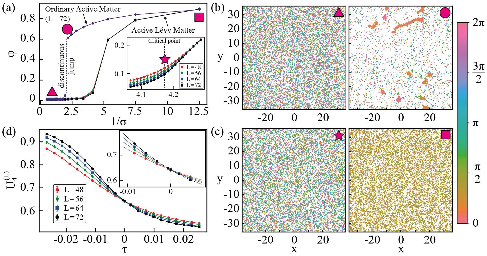
Figure 2: Finite size scaling analysis of the microscopic model of active Lévy matter. We run $300$ independent numerical simulations of the Langevin equations (1) in a square box of linear length $L=\{48,56,64,72\}$ with periodic boundary conditions. Other parameters are $\rho=2$, $\gamma=0.25$ and $\alpha=1/2$ ($\alpha=1$ for Vicsek type dynamics). The model is initialized in the homogeneously disordered phase and updated for $2.5\times 10^{6}$ time sweeps, which are sufficient for equilibration Cairoli and Lee . (a) Time averaged polar order parameter $\varphi$ vs. the rotational noise strength $\sigma$. (b) Snapshots of the system configuration for ordinary active matter in the disordered phase (left) and in the unstable region at the onset of the transition (right). (c) Similar snapshots for active Lévy matter at the critical point (left) and in the ordered phase (right). (d) Binder cumulant $U_{4}^{(L)}$ vs. the distance from the critical noise strength $\tau$. Inset: Quadratic fits of Binder cumulant curves around the critical point. In panels (a) and (d) error bars are plotted denoting 1 s.e.m.; in the inset of panel (d) we also plot 95% confidence bands on the best fit lines.

Similar to ordinary active fluids, the hydrodynamic behaviour of the system around the onset of collective motion is dictated only by the lower order modes Bertin et al. (2006); Peruani et al. (2008); Bertin et al. (2009); Bertin (2017); Lee (2010); Peshkov et al. (2014), because all the higher-order modes are suppressed by the “mass” term $\propto\sigma m^{2}$ and by the homogeneous term $\propto\Upsilon_{0}k^{\alpha}$ resulting from the fractional operator (4). We therefore adopt the same approximation strategy used in ordinary active matter, i.e., we assume that $\hat{f}_{m}\approx 0$ for $m\geq 3$ and $\partial_{t}\hat{f}_{2}\approx 0$. The equation for $\hat{f}_{2}$ then becomes algebraic and can be solved. Using this exact result and re-expressing the equations for $f_{0}$ and $f_{1}$ in terms of the density, director, and nematic fields, we obtain the hydrodynamic EOM, to order $k^{\alpha}$, Cairoli and Lee

$$(\partial_{t}+\Upsilon_{0}\mathbb{D}^{\alpha})\rho=2\Upsilon_{1}\mathbb{I}^{1-\alpha}(\nabla\cdot\mathbf{p})-\lambda_{2}\mathbb{I}^{2-\alpha}(\nabla\cdot\boldsymbol{\Xi}_{0}),$$ (8)

$$(\partial_{t}+\Upsilon_{0}\mathbb{D}^{\alpha})\mathbf{p}=[\kappa_{0}(\rho)-\xi|\mathbf{p}|^{2}]\mathbf{p}+\Upsilon_{1}\mathbb{I}^{1-\alpha}\nabla\rho$$

$$\quad+\lambda_{1}\mathbb{I}^{1-\alpha}\boldsymbol{\Xi}_{0}-\Upsilon_{2}\mathbb{I}^{2-\alpha}\nabla^{2}\mathbf{p}+\lambda_{3}\mathbb{I}^{3-\alpha}\boldsymbol{\Xi}_{1}-\textbf{Q}\mathbf{p}\ ,$$ (9)

where $\mathbb{I}^{\beta}$ is the fractional Riesz integral defined by its Fourier transform $\mathbb{I}^{\beta}h(\mathbf{r})\rightarrow k^{-\beta}\hat{h}(\mathbf{k})$ (for $\mathrm{Re}\,{\beta}>0$ and $h$ a test function), and $\mathbb{D}^{\beta}$ is the corresponding fractional derivative whose Fourier representation is $\mathbb{D}^{\beta}h(\mathbf{r})\rightarrow k^{\beta}\hat{h}(\mathbf{k})$ Samko et al. (1993); Tarasov (2011). The operators $\mathbb{I}^{\beta}$ and $\mathbb{D}^{\beta}$ are the inverses of each other. In Eqs (8) and (9), we have also defined the following non-linear $(\mathbf{r},t)$-dependent vector fields

$$\boldsymbol{\Xi}_{0} \equiv 2[(\mathbf{p}\cdot\nabla)\mathbf{p}+(\nabla\cdot\mathbf{p})\mathbf{p}]-\nabla|\mathbf{p}|^{2}\ ,$$ (10)

$$\boldsymbol{\Xi}_{1} \equiv(\mathbf{p}\cdot\nabla)\nabla^{2}\mathbf{p}+(\mathbf{p}\times\nabla)\times\nabla^{2}\mathbf{p}$$

$$\quad+3[(\nabla\cdot\mathbf{p})\nabla^{2}\mathbf{p}+(\boldsymbol{\omega}\times\nabla^{2}\mathbf{p})-(\boldsymbol{\omega}\cdot\nabla)\boldsymbol{\omega}]\ ,$$ (11)

where $\boldsymbol{\omega}(\mathbf{r},t)\equiv\nabla\times\mathbf{p}$ is the vorticity field. The nematic tensor Q is specified by its components $\text{Q}_{xx}=\mathcal{Q}_{1}=-\text{Q}_{yy}$ and $\text{Q}_{xy}=\mathcal{Q}_{2}=\text{Q}_{yx}$, which are

$$\mathcal{Q}_{i} =-B_{0}\mathbb{D}^{\alpha}\text{M}_{ij}p_{j}+\frac{\lambda_{1}}{2}\mathbb{I}^{1-\alpha}\text{T}_{ij}p_{j}-\frac{\lambda_{2}}{4}\mathbb{I}^{2-\alpha}\text{T}_{ij}\partial_{j}\rho$$

$$\quad+\frac{\lambda_{3}}{4}\mathbb{I}^{3-\alpha}\text{T}_{ij}\nabla^{2}p_{j}-B_{4}\mathbb{I}^{4-\alpha}\text{T}_{ij}\Xi_{1j}\ ,$$ (12)

where $i,j=1,2$ and $p_{1}$ and $p_{2}$ are the components of $\mathbf{p}$ along the $x$ and $y$ axis, respectively. In the above, we have also defined the tensor function $\text{M}_{ij}\equiv p_{1}\delta_{ij}+p_{2}\epsilon_{ij}$ and the differential operator $\text{T}_{ij}\equiv\partial_{x}\delta_{ij}+\partial_{y}\epsilon_{ij}$, where $\delta_{ij}$ is the Kronecher symbol and $\epsilon_{ij}$ is the generator of counter-clock wise rotations, with $\epsilon_{11}=0=\epsilon_{22}$ and $\epsilon_{21}=1=-\epsilon_{12}$. Furthermore, we have introduced the density-dependent quantity $\kappa_{0}(\rho)\equiv-\sigma+(\gamma\rho)/2$ and the coefficients

$$\lambda_{1} \equiv\frac{\gamma\Upsilon_{1}}{4\sigma}\ ,\ \lambda_{2} \equiv\frac{\gamma\Upsilon_{2}}{2\sigma}\ ,\ \lambda_{3} \equiv\frac{\gamma\Upsilon_{3}}{2\sigma},$$ (13)

$$B_{0} \equiv\frac{\gamma^{2}\Upsilon_{0}}{32\sigma^{2}}\ ,\ B_{4} \equiv\frac{\gamma^{2}\Upsilon_{4}}{16\sigma^{2}}\ ,\ \xi \equiv\frac{\gamma^{2}}{8\sigma}\ .$$ (14)

The hydrodynamic EOM (8) and (9) are our first main result and may be viewed as the counterpart of the Toner-Tu equations for ALM. We note that, for $\alpha=1$, we have $\Upsilon_{i}=0$ for all $i\neq 1$ and $\Upsilon_{1}=-1/2$ Cairoli and Lee , so that (8) and (9) are reduced to a version of the Toner-Tu equations Toner and Tu (1995, 1998); Toner (2012) without the ordinary viscosity term, which is absent because of the truncation in the wavenumber $k$.

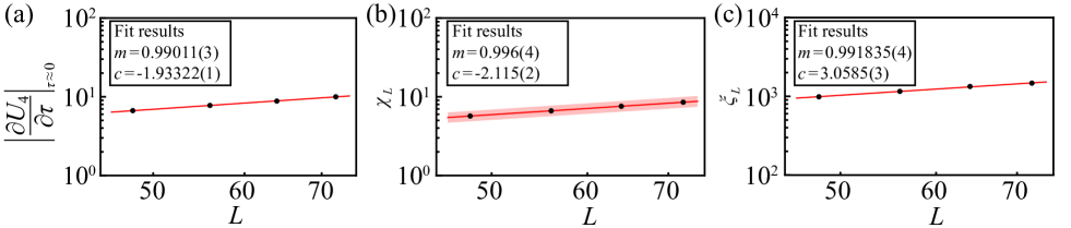
Figure 3: Numerical estimation of static and dynamic critical exponents for the order-disorder transition in active Lévy matter. Model parameters are $\rho=2$, $\gamma=0.25$ and $\alpha=1/2$. The simulation data (in logarithmic scales) are fitted with the linear function $m\,L+c$ by using a weighted least squares method. Error bars are plotted denoting 1 s.e.m.; 95% confidence bands on fit parameters are also shown. (a) Gradient of the Binder cumulant at criticality $|\partial U_{4}^{(L)}/\partial\tau|_{\tau\simeq 0}$ vs. the system size $L$. (b) Susceptibility at criticality $\chi_{L}$ vs. $L$. (c) Correlation time of the polar order parameter $\xi_{L}$ at criticality vs. $L$.

At the mean-field level, our EOM predict the same phase behaviour of the Toner-Tu equations, because all terms involving (integral or fractional) spatial derivatives can be ignored. Equations (8) and (9) thus indicate (a) the disordered phase with $\mathbf{p}^{*}=0$ for $\sigma\geq\sigma_{t}$; and (b) the ordered phase with $\mathbf{p}^{*}\equiv\sqrt{8\sigma\kappa_{0}(\rho^{*})/\gamma^{2}}\mathbf{e}_{\parallel}$, where $\mathbf{e}_{\parallel}$ denotes the arbitrary direction of spontaneous symmetry breaking for $\sigma<\sigma_{t}$. The density dependent threshold rotational noise strength is $\sigma_{t}(\rho^{*})\equiv\gamma\rho^{*}/2$.

The mean-field description is known to be inadequate at the onset of collective motion for ordinary active matter due to the emergence of the characteristic banding instability, which manifests itself as a longitudinal instability (i.e., along the direction of collective motion), with the $k\rightarrow 0$ mode being the most unstable. Strikingly, this is no longer true in ALM. To demonstrate this, we perturb the hydrodynamic fields $\rho$ and $\mathbf{p}$ as $\rho^{*}+\delta\rho_{0}e^{st+i\mathbf{q}\cdot\mathbf{r}}$ and $\mathbf{p}^{*}+\delta\mathbf{p}_{0}e^{st+i\mathbf{q}\cdot\mathbf{r}}$, respectively, and solve (8) and (9) at the linear level in $\delta\rho_{0}$ and $\delta\mathbf{p}_{0}$. Eliminating them then yields the dispersion relation with solutions $s_{\pm}(\mathbf{q})$ such that $\mathrm{Re}\,{s_{+}}>\mathrm{Re}\,{s_{-}}$. The spatially homogeneous phases predicted by the mean-field theory are only stable if $\mathrm{Re}\,{s_{+}}<0$. Similar to ordinary active fluids, we find that the disordered phase is stable against perturbations in all directions Cairoli and Lee . However, for the ordered phase, in the hydrodynamic limit, we obtain Cairoli and Lee

$$\mathrm{Re}\,{(s_{-})} \simeq-2\kappa_{0}(\rho^{*})+\mathcal{O}(q^{\alpha})\ ,$$ (15)

$$\mathrm{Re}\,{(s_{+})} \simeq(-\Upsilon_{0}+2\Upsilon_{2})q^{\alpha}+\mathcal{O}(q^{2\alpha})\ .$$ (16)

The first eigenvalue, $s_{-}$, always has a negative real part and describes the fast relaxation of small perturbations from $\mathbf{p}^{*}$. For normal active fluids, the real part of the second eigenvalue, $s_{+}$, is always positive as the system approaches the onset of collective motion Bertin et al. (2006), indicating the banding instability that renders the transition first-order Grégoire and Chaté (2004); Chaté et al. (2008); Solon and Tailleur (2013, 2015). For ALM, instead, this eigenvalue has a negative real part because $\Upsilon_{0}>2\Upsilon_{2}$ for all $0<\alpha<1$. Therefore, the banding instability is made stable by the Lévy motion of the active particles. Furthermore, we can demonstrate that transversal perturbations (i.e., orthogonal to the direction of collective motion) are also suppressed Cairoli and Lee . As a result, in ALM, the ordered phase always remains stable at the onset of collective motion in the hydrodynamic limit, thus rendering the order-disorder phase transition potentially critical. These predictions represent the second main result of our work.

$\nu$	$\beta/\nu$	$\gamma/\nu$	$z$
$1.00999(3)$	$0.497(1)$	$0.996(4)$	$0.991835(4)$

Table 1: Numerical estimates of the critical exponents for $\alpha=1/2$. Errors are expressed as 1 s.e.m..

We now investigate the critical behavior predicted by our theory with numerical simulations. We focus here on the particular value $\alpha=1/2$ Cairoli and Lee . We first note that the criticality of the phase transition manifests in the smooth approach of the time averaged polar order parameter $\varphi$ to zero as the rotational noise is increased, as opposed to the abrupt jump found in ordinary active matter, which is characteristic of a first-order transition (Fig. 2a). Snapshots of the system configuration also confirm these predictions (Figs. 2b and 2c). We now characterize the critical exponents of the phase transition by performing a finite size scaling analysis Landau (2014). Specifically, we first estimate the asymptotic critical noise strength at fixed density, $\sigma_{\star}$, by identifying the crossing of the Binder cumulant $U_{4}^{(L)}\equiv\langle\varphi^{2}\rangle_{L}^{2}/\langle\varphi^{4}\rangle_{L}$ for different system sizes $L$ (Fig. 2d). Here, $\langle\cdot\rangle_{L}$ denotes the ensemble average taken at finite system size $L$. We estimate: $\sigma_{\star}=0.239816(2)$ (error is 1 s.e.m.). Using the scaling relation $|\partial U_{4}^{(L)}/\partial\tau|_{\tau\simeq 0}\propto L^{1/\nu}$, where $\tau\equiv-1+\sigma/\sigma_{\star}$, we can estimate directly the static exponent $\nu$ (Fig. 3a). In addition, using the scaling relations for the polar order parameter at criticality $\varphi_{\star}\propto L^{-\beta/\nu}$ and that for the susceptibility $\chi_{L}\propto L^{\gamma/\nu}$, with $\chi_{L}\equiv L^{2}(\langle\varphi_{\star}^{2}\rangle_{L}-\langle\varphi_{\star}\rangle_{L}^{2})$, we can estimate the ratios of static critical exponents $\beta/\nu$ and $\gamma/\nu$ (Fig. 3b). To estimate the dynamic exponent $z$, we use the scaling relation for the correlation time of the polar order parameter $\xi_{L}\propto L^{z}$ (Fig. 3c). The estimates obtained are summarized in Table 1. The numerical characterization of the critical properties of the order-disorder transition is our third main result. Intriguingly, these estimates for $\alpha=1/2$ seem to indicate that the static properties of the critical transition in ALM (for the particular $\alpha$ considered here) belongs to the same universality class of the equilibrium model in two spatial dimensions with long-range interaction energy $\propto 1/|\mathbf{r}_{ij}|^{2+2\alpha}$ and $n$-component order parameter Fisher et al. (1972); Suzuki (1973). Elucidating analytically this connection by employing dynamic renormalization group methods, similarly to what was accomplished for ordinary active matter in incompressible conditions Chen et al. (2015, 2016, 2018), is an interesting open problem that we aim to elucidate in future investigations.

In this Letter, we derived the first hydrodynamic description of ALM, which generalizes the conventional theory of active fluids by incorporating Lévy stable distributed fluctuations with diverging variance. We then revealed that, unlike ordinary polar active matter, the order-disorder transition in ALM is critical and estimated the corresponding critical exponents numerically. Our work highlights the novel physics exhibited by active matter models integrating both anomalous diffusive motility and inter-particle interactions. Interesting future directions include the investigation of the effects of Lévy displacement dynamics on collective phenomena other than collective motion such as active turbulence Dombrowski et al. (2004); Hernandez-Ortiz et al. (2005); Sokolov et al. (2007); Aranson et al. (2007); Saintillan and Shelley (2007); Wolgemuth (2008); Sanchez et al. (2012); Wensink et al. (2012); Doostmohammadi et al. (2018) and motility-induced phase separation Tailleur and Cates (2008); Fily and Marchetti (2012); Redner et al. (2013); Cates and Tailleur (2015), as well as their relevance to biological systems Zaburdaev et al. (2015).