Dynamics of a Massive Binary at Birth

Abstract

Almost all massive stars have bound stellar companions, existing in binaries or higher-order multiples[1, 2, 3, 4, 5]. While binarity is theorized to be an essential feature of how massive stars form[4], essentially all information about such properties is derived from observations of already formed stars, whose orbital properties may have evolved since birth. Little is known about binarity during formation stages. Here we report high angular resolution observations of 1.3 mm continuum and H30$\alpha$ recombination line emission, which reveal a massive protobinary with apparent separation of 180 au at the center of the massive star-forming region IRAS07299-1651. From the line-of-sight velocity difference of 9.5$\>\mbox{km s}^{-1}$ of the two protostars, the binary is estimated to have a minimum total mass of 18 solar masses, consistent with several other metrics, and maximum period of 570 years, assuming a circular orbit. The H30$\alpha$ line from the primary protostar shows kinematics consistent with rotation along a ring of radius of 12 au. The observations indicate that disk fragmentation at several hundred au may have formed the binary, and much smaller disks are feeding the individual protostars.

Star and Planet Formation Laboratory, RIKEN Cluster for Pioneering Research, Hirosawa 2-1, Wako-shi, Saitama 351-0198, Japan

Department of Space, Earth & Environment, Chalmers University of Technology, SE-412 96 Gothenburg, Sweden

Department of Astronomy, University of Virginia, Charlottesville, VA 22904-4325, USA

Department of Earth and Space Science, Osaka University, Toyonaka, Osaka 560-0043, Japan

Chile Observatory, National Astronomical Observatory of Japan, Mitaka, Tokyo 181-8588, Japan

SOFIA-USRA, NASA Ames Research Center, MS 232-12, Moffett Field, CA 94035, USA

INAF – Osservatorio Astrofisico di Arcetri, Largo E. Fermi 5, 50125 Firenze, Italy

Department of Astronomy and Steward Observatory, University of Arizona, 933 N Cherry Ave, Tucson, AZ, 85721, USA

Departamento de Astronomía, Universidad de Chile, Casilla 36-D, Santiago, Chile

We observed infrared source IRAS07299-1651, thought to be a massive protostar[2], $1.68\>$kpc away[8], with the Atacama Large Millimeter/Submillimeter Array (ALMA) (Methods). At $\sim 10^{4}\>{\rm{au}}$ scales, the low-resolution ($0.22^{\prime\prime}\times 0.15^{\prime\prime}$, i.e., $370\>\mbox{au}\times 260\>\mbox{au}$) 1.3 mm continuum image exhibits several stream-like structures connecting to the central source (Figure 1a). The mass of these structures $>500\>$au from the continuum peak is $3.8-8.0\>M_{\odot}$ (Methods). The high angular resolution ($35\>\mathrm{mas}\times 29\>\mathrm{mas}$, i.e., $59\>\mbox{au}\times 49\>\mbox{au}$) 1.3 mm continuum observation filters out large-scale emission and resolves the central peak into two compact, marginally-resolved sources with apparent separation of 180 au (Figure 1b). The fluxes of the brighter, western Source A and the fainter, eastern Source B are 51 and 18 mJy, respectively.

H30$\alpha$ hydrogen recombination line (HRL) emission is detected towards both sources, with positions and sizes coinciding closely with the continuum emission (Figure 1b). The strong HRL emission suggests that the small-scale 1.3 mm continuum has significant contribution from ionized gas free-free emission, in addition to dust emission (Methods). H30$\alpha$ spectra from the continuum peak positions are shown in Figure 2. They are well fit ($<$10% deviation) with Gaussians from which central velocities are determined: $15.5\pm 1.1\>\mbox{km s}^{-1}$ for A and $25.0\pm 1.6\>\mbox{km s}^{-1}$ for B (Methods). Source A’s spectrum exhibits slight asymmetry, perhaps caused by small portions of optically thick gas, or different internal velocity components. Assuming the H30$\alpha$ central velocities trace the protostar radial velocities (Methods), the velocity difference between the two sources may then be due to binary orbital motion, and can thus constrain the system mass and orbital properties.

First assuming circular (zero eccentricity) orbits, expected to be a good approximation for a binary forming by disk fragmentation, i.e., via accretion of gas on near circular disk orbits[4], then the minimum source separation is their apparent separation $a_{0}=180\pm 11\>\mbox{au}$, with uncertainty dominated by that of source distance[8]. Combining with the projected velocity difference $\Delta v=9.5\pm 1.9\>\mbox{km s}^{-1}$, yields a maximum orbital period $P_{0}=(5.7\pm 1.2)\times 10^{2}$ years and minimum total system mass $M_{0}=18.4\pm 7.4\>M_{\odot}$. For an elliptical orbit with eccentricity $e$, the minimum system mass is $M_{\mathrm{min}}=M_{0}/(1+e)$. The minimum mass for a bound system is therefore $M_{0}/2=9.2\pm 3.7\>M_{\odot}$. For circular orbits, Figure 3 displays allowed distributions of orbital period and system mass, showing how changes in orbital plane inclination and position angle cause the system mass to be $>M_{0}$ and the orbital period to be $<P_{0}$. Supplementary Figure 1 shows similar distributions for elliptical orbits. Typical example orbits with $e\leq 0.2$ are displayed in Figure 1(c). Assuming the center of mass radial velocity of the binary is the same as the molecular cloud systemic velocity, we also constrain the binary mass ratio from the determined source radial velocities (Methods). With $V_{\mathrm{sys}}=16.5-18~{}\mbox{km s}^{-1}$, the probable range for the binary mass ratio is up to $\sim 0.7$ (Figure 3c).

We also use the HRL-derived free-free emission to independently estimate protostar masses and thus further constrain binary orbital properties. We estimate free-free components in the 1.3 mm continuum to be 39 mJy and 4 mJy in Sources A and B (Methods). If free-free emissions arise from regions ionized by stellar radiation, implied zero-age main-sequence (ZAMS) masses are $12.5\>M_{\odot}$ (Source A) and $10\>M_{\odot}$ (Source B), i.e., spectral types B0.5 and B1 (Methods), suggesting indeed two massive stars in formation. However, the protostars may not yet have contracted to the ZAMS. Then free-free emission implies masses $8-19\>M_{\odot}$ for A and $7-17\>M_{\odot}$ for B (Methods). The concentrated HRL emission morphology suggests the ionized gas is confined close to the protostars, consistent with theoretical models for the above mass estimates[9]. The total system masses from these estimations are also consistent with the minimum mass from orbital constraints.

As Figure 3 shows, for the system mass of $\sim 22.5~{}M_{\odot}$ estimated from free-free emission based on ZAMS models, orbital period $P$ is $510-570\>$yr, orbital plane is close to edge-on (inclination between orbital plane and sky plane $i>70^{\circ}$), and position angle of orbital plane similar (within $5^{\circ}$) to the A-B axis. Considering uncertainties in determination of protostellar masses ($15-36\>M_{\odot}$), the orbital period can be shorter ($\sim 400\>$yr) and orbital plane inclination can be $i>50^{\circ}$, but orbital plane position angle remains within $\sim 15^{\circ}$ relative to the A-B axis. The ranges of orbital properties increases if elliptical orbits are considered (Supplementary Information).

The observed H30$\alpha$ line widths, FWHM of $39$ and $55\>\mbox{km s}^{-1}$ of A and B, are expected to be dominated by dynamics of turbulence, rotation, inflow or outflow, rather than by thermal or pressure broadening, unlike lower frequency H$n\alpha$ $(n\gg 30)$ lines[10]. Velocity gradients are seen, especially around the primary (Supplementary Figures 2 and 3), indicating ordered motion of ionized gas. To understand such motion around the primary, in each velocity channel with H30$\alpha$ peak emission $>20\sigma$, a 2D Gaussian fit is performed to determine the emission’s centroid position (Figure 4 and Methods). Centroid positions show a very organized pattern along a half ellipse with center close to the continuum peak. The northern half of the ellipse is blue-shifted; the southern is red-shifted. The most blue and red-shifted emission is at the ends of the major axis. One way to explain such a pattern is by an inclined rotating ring: we fit centroid positions and intensities with such a model (Methods). The best fit model (Figure 4) has a ring with radius $R_{\mathrm{ring}}=7\pm 1\>\mathrm{mas}$, i.e., 12 au, rotating at velocity $V_{\mathrm{rot}}=21\pm 2\>\mbox{km s}^{-1}$, corresponding to a central mass of $6\pm 2\>M_{\odot}$, assuming Keplerian rotation.

This dynamic mass of the primary is consistent with the minimum system mass constrained from orbital motion (assuming similar masses of the binary members). It is somewhat smaller than that estimated from free-free emission ($12.5^{+6.5}_{-4.5}\>M_{\odot}$), so the rotation might be sub-Keplerian. Such a rotating structure is likely to either be part of the accretion disk that has been ionized[11, 12] or from a slow, rotating ionized disk wind, which have been seen in some other systems[13, 14]. The small-scale dust continuum emissions are found to be optically thick, suggesting structures with high mass surface densities of $\sim 1\times 10^{2}\>\mathrm{g}\>\mathrm{cm}^{-2}$ around the protostars (Methods), which are likely to be individual circumstellar disks. If the ionized gas ring is confined within an opaque dusty disk that is thick and flared, due to the inclination, the front side of the ionized ring would be blocked by the outer part of such disk. This can naturally explain why only the eastern half of the ring, which is the far side, is seen in H30$\alpha$ emission.

The morphology and kinematics of the large sclae structures appear complex, as illustrated by zeroth and first moment maps of CH₃OH line emission (Supplementary Figure 4a). We use a model of rotating-infall[1] to explain the kinematic features of one of the main structures (Supplementary Information). This model requires a central mass of $27\pm 6~{}M_{\odot}$, consistent with the minimum system mass derived from orbital motion and also the total protostellar mass estimated from free-free emission. The radius of the centrifugal barrier is estimated to be $840~{}\mbox{au}$, moderately larger than the binary separation, as expected in disk fragmentation models[4]. A circumbinary disk may have formed inside the centrifugal barrier, which feeds one or both members of the binary. However, it is difficult to separate such disk emission from that of the infalling streams due to projection effects. Also, there is no distinct kinematic signature of a circumbinary disk detected in CH₃OH emission.

Placing our results in context, so far only very few massive protobinary systems have been identified: IRAS20126+4104 (apparent separation of 850 au) by NIR imaging[16], G35.20-0.74 (800 au) and NGC7538-IRS1 (430 au) by cm continuum observations[17, 18], and IRAS17216-3801 (170 au) by NIR interferometry[19]. Only the separation information was used to define these binary systems. Our study is the first, to our knowledge, measurement of dynamical constraints on the or- bit of a forming massive binary. In IRAS07299-1651 we are witnessing massive binary formation and accretion on multiple spatial scales, from infalling streams at $1,000-10,000$ au, to formation of a massive binary system on $100-1,000$ au scales, and to accretion disks feeding individual stars on 10 au scales.

Overall we consider these results support a scenario of disk fragmentation for massive binary formation[4]. First, large-scale structures are seen that are consistent with infall in the core envelope to a central disk, and the observed separation of the binary is moderately smaller than the inferred centrifugal barrier. Second, the secondary-to-primary mass ratio is about 0.8 based on free-free emission and ZAMS models, or up to about 0.7 based on the center of mass velocity, close to asymptotic values seen in simulations of binary formation via disk fragmentation. This is caused by the secondary growing preferentially from a circumbinary disk, since it is further from the center of mass. Production of near equal mass high-mass stars by turbulent fragmentation, i.e., independent formation events that happen to form near each other in a bound state, is unlikely, given the rarity of massive stars. Third, only very few protostellar sources are detected in the region (Supplementary Information), rather than a rich cluster of forming stars, which is consistent with limited fragmentation in Core Accretion models for massive star formation[20], perhaps due to magnetic fields, radiative heating or the tidal fields from an already formed central massive star or binary. In this case, fragmentation to produce the binary at its observed scale arises from gravitational instability in a massive disk around the original primary. The current circumbinary disk could be much less massive than this earlier disk. A much higher degree of fragmentation is expected if the region is undergoing widespread turbulent fragmentation and in Competitive Accretion models of massive star formation[21].

There are, however, caveats and open questions associated with the disk fragmentation interpretation. One concerns the potential misalignment between the orbital plane and the rotational structure around Source A. The angle between these two planes is $>54^{\circ}$ (Methods). Furthermore, the direction of the large scale structures appears to be similar to that of the rotational structure around Source A and different from that of the orbital plane. While such misalignment is often considered as an indicator of turbulent fragmentation of binary formation, it may also be caused by changes in the orientation of the angular momentum of accreting gas at these various scales, perhaps inherited from different infalling components of a turbulent core, where one expects substructure in the infall envelope[22]. Indeed the infalling material appears highly structured and would have different angular momentum directions, so disk orientation should fluctuate during the formation process. Such misalignment between circumbinary and circumstellar disks have been indicated by recent observations of both low and high-mass sources[19, 23]. Future observations may test the disk fragmentation scenario by determining whether the orbit is close to circular or not. Finally, larger samples need to be observed with these methods to determine how common these features are during massive star formation.

Correspondence and requests for materials should be addressed to Y.Z. (email: yichen.zhang@riken.jp).

The authors thank Nami Sakai for valuable discussions. ALMA is a partnership of ESO (representing its member states), NSF (USA) and NINS (Japan), together with NRC (Canada), MOST and ASIAA (Taiwan), and KASI (Republic of Korea), in cooperation with the Republic of Chile. The Joint ALMA Observatory is operated by ESO, AUI/NRAO and NAOJ. The National Radio Astronomy Observatory is a facility of the National Science Foundation operated under cooperative agreement by Associated Universities, Inc. Y.Z. acknowledges support from RIKEN Special Postdoctoral Researcher Program. J.C.T. acknowledges support from NSF grant AST1411527 and ERC Advanced Grant project MSTAR. K.E.I.T acknowledges support from NAOJ ALMA Scientific Research Grant Number 2017-05A. D.M. and G.G. acknowledge support from CONICYT project Basal AFB-170002.

Y.Z. led part of the ALMA observations, performed the data analysis, led the discussions, and drafted the manuscript. J.C.T. led part of the ALMA observation, and participated in the discussions and drafting manuscript. K.E.I.T. contributed to the discussions. The rest of the authors discussed the results and commented on the manuscript.

The authors declare that they have no competing financial interests.

Figure 1: Maps of the continuum and H30$\alpha$ line emissions. (a): The 1.3 mm continuum map is shown in color scale on the background image. The synthesized beam (shown in box in bottom-left corner) is $0.22^{\prime\prime}\times 0.15^{\prime\prime}$. (b): The 1.3 mm continuum map (color scale and white contours) and the H30$\alpha$ line emission (dashed orange contours) on small scales revealing a binary system. The continuum contour levels are 3$\sigma$, 6$\sigma$, 12$\sigma$, 24$\sigma$, …, with $1\sigma=1.6~{}\mbox{K}$ (0.07 $\mbox{mJy beam}^{-1}$). The H30$\alpha$ line emission is integrated in the velocity range of $-30~{}\mbox{km s}^{-1}<V_{\mathrm{lsr}}<55~{}\mbox{km s}^{-1}$, and the contour levels are 5$\sigma$, 10$\sigma$, 20$\sigma$, …, with $1\sigma=280~{}\mbox{K km s}^{-1}$ (13 $\mbox{mJy beam}^{-1}$ $\mbox{km s}^{-1}$). The synthesized beam (shown in bottom-left corner) is $35~{}\mathrm{mas}\times 29~{}\mathrm{mas}$. (c): Examples of possible binary orbits (relative orbits of Source B with respect to Source A) of different system masses shown in color. Orbits with system mass ranging from 5 to 35 $M_{\odot}$ and eccentricity ranging from $e=0$ to 0.2 are shown. The red ellipse around Source A is the rotational structure fitted from H30$\alpha$ emission centroids. The R.A. and Dec. offsets are relative to the continuum peak position of Source A ($7^{\mathrm{h}}32^{\mathrm{m}}09^{\mathrm{s}}.785,-16^{\circ}58^{\prime}12^{\prime\prime}.148$).

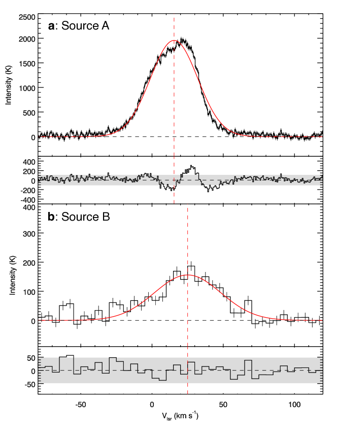
Figure 2: H30$\alpha$ line spectra at the continuum peak positions of Source A (panel a) and Source B (panel b). The r.m.s. noise levels are marked by the error bar in each velocity channel. The red solid curves are fitted Gaussian profiles with the central velocities indicated by the red dashed lines. The residual differences between the observed spectra and fitted Gaussian profiles are also shown below the spectra. The shaded regions indicate the $3\sigma$ noise levels.

Figure 3: (a): The distribution of the possible binary properties in the space of system mass and orbital period. The color shows the inclination of the orbital plane relative to the plane of sky. Only circular orbits are considered here. The data point and error bars correspond to the system mass, orbital period and their uncertainties, assuming an edge-on circular orbit with the apparent separation of the two sources as their true separation. The dashed vertical line and the shaded regions indicate the system mass and its uncertainties derived from the continuum and H30$\alpha$ line observations. The solid lines show the locations of orbits with different separations, as labelled. (b): Same as panel a, with the color showing the position angle of the intersection line between the orbital plane and the sky plane, with respect to the position angle of the line connecting Source A and B. (c): The dependence of binary mass ratio ($M_{B}/M_{A}$) on the center of mass radial velocity, calculated from the source radial velocities and uncertainties. The solid black curve and the dark shaded region show this relation with $v_{A}=15.5\pm 1.1~{}\mbox{km s}^{-1}$, and the dashed black curve and the light shaded region show this relation with $v_{A}=14.5\pm 1.1~{}\mbox{km s}^{-1}$, considering $v_{A}$ is likely to be more blue-shifted than the spectrum central velocity due to the slight asymmetry in the spectrum. The blue region between the two vertical dashed lines shows the range of cloud systemic velocities measured from various molecular lines. The solid red line and the red region show the mass ratio derived from H30$\alpha$ intensities and its uncertainties.

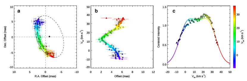
Figure 4: a) Distribution of the centroids of H30$\alpha$ emission in Source A in each velocity channel. The centroids (triangles with error bars) are determined by a 2D Gaussian fit to the H30$\alpha$ emission in each channel. Only channels with peak H30$\alpha$ intensities higher than 20$\sigma$ ($1\sigma=1.8~{}\mbox{mJy beam}^{-1}$) are included. The R.A. and Dec. offsets are relative to the continuum peak position. Line-of-sight velocities are shown by the color scale. The colored circles are the predicted centroid distribution of the best fit model of an inclined rotating ring. The actual projected shape of the best fit ring is shown by the black ellipse, where the emission comes from the eastern half (shown with a solid line). The center of the fitted ring is marked by the star. b) Distances of the centroids from the continuum peak position with their line-of-sight velocities, compared with the best-fit model. c) Scaled centroid intensities compared with the prediction of the best-fit model. The meaning of the symbols in Panels (b) and (c) are same as those in panel (a).

0.1 Observations.

The observations were carried out with ALMA in Band 6 on April 3, 2016 with the C36-3 configuration, on Sept. 17, 2016 with the C36-6 configuration, and on Sept, 23, 2017 with the C40-9 configuration. The total integration time is 3, 6, and 18 min in the three configurations. 36 antennas were used and the baselines range from 15 m to 462 m in the C36-3 configuration, 36 antennas were used and the baselines range from 15 m to 3.2 km in the C36-6 configuration, and 40 antennas were used and the baselines range from 41 m to 12 km in the C40-9 configuration. J0750+1231 was used for bandpass and flux calibration, while J0730-1141 and J0746-1555 were used as phase calibrators. The source was observed with single pointings, and the primary beam size (half power beam width) was 22.9^′′. The data from C36-3 and C36-6 configurations were combined (referred to as “low-resolution” data), while the data from C40-9 configuration (referred to as the “high-resolution” data) were not combined with other data, in order to emphasize the small-scale structures. The largest recoverable scales of the low- and high-resolution data are about 11^′′ and 3.9^′′, respectively.

A spectral window with a bandwidth of 2 GHz was used to map the 1.3 mm continuum. The H30$\alpha$ line was observed with velocity resolution of about $0.7~{}\mbox{km s}^{-1}$, and the molecular lines with about $0.2~{}\mbox{km s}^{-1}$. The molecular lines are only detected in the low-resolution observation, and here we only show the CH₃OH $4(2,2)-3(1,2)$ line data, as other detected molecular lines such as the H₂CO $3(2,1)-2(2,0)$ line and the C¹⁸O $(2-1)$ line show similar behaviors (these data will be presented in a separate paper).

The data were calibrated and imaged in CASA[1]. Self-calibration was applied to both the continuum and line data by using the continuum data after the normal calibration. The self-calibration was performed for the data of three configurations separately. The CLEAN algorithm was used to image the data, using robust weighting with the robust parameter of 0.5. The resultant synthesized beams are $0.035^{\prime\prime}\times 0.029^{\prime\prime}$ for the high resolution continuum data, $0.035^{\prime\prime}\times 0.030^{\prime\prime}$ for the high resolution H30$\alpha$ data, $0.22^{\prime\prime}\times 0.15^{\prime\prime}$ for the low resolution continuum data, and $0.25^{\prime\prime}\times 0.17^{\prime\prime}$ for the low-resolution CH₃OH data.

The continuum peaks of the two sources are derived to be at $(\alpha_{2000},\delta_{2000})_{\mathrm{Source~{}A}}=(7^{\mathrm{h}}32^{\mathrm{m}}09^{\mathrm{s}}.786$, $-16^{\circ}58^{\prime}12^{\prime\prime}.146)$ and $(\alpha_{2000},\delta_{2000})_{\mathrm{Source~{}B}}=(7^{\mathrm{h}}32^{\mathrm{m}}09^{\mathrm{s}}.793$, $-16^{\circ}58^{\prime}12^{\prime\prime}.196)$ from the high-resolution data using CASA imfit. There is a third continuum source at 8.5^′′ ($1.4\times 10^{4}~{}\mbox{au}$) to the northeast of the binary system, detected in both low and high resolution data (not shown in Figure 1). In the high-resolution data, the source has a peak brightness temperature of 30 K and a resolved size of about 200 au, i.e., much fainter and more extended than the binary sources. No H30$\alpha$ emission is detected toward this source. Multiplicity in this region is discussed in Supplementary Information.

0.2 Estimating the line-of-sight velocities of the protostars.

We fit the H30$\alpha$ spectra at the continuum peak positions of the two sources with Gaussian profiles to determine the central velocities. The uncertainties are estimated by adding random noise (same as the r.m.s noise level of each channel) to the fitted Gaussian profiles, repeating the fitting many times, and then calculating the standard deviation of the fitted central velocities. For Source A, the spectrum deviates slightly from a symmetric Gaussian profile, but the fractional difference of the data from the best-fit Gaussian profile is only 7.8% (only the parts which have deviations $>3\sigma$ are included). For Source B, the deviations of the data from the Gaussian profile are all within the $3\sigma$ level. The determined central velocities are $v_{A}=15.5\pm 0.064\>\mbox{km s}^{-1}$ for Source A and $v_{B}=25\pm 1.2\>\mbox{km s}^{-1}$ for Source B.

For Source A, we further add some perturbation on the fitted Gaussian profile to simulate the effects of the asymmetry on the determination of central velocity. The perturbation has a form of sine function with a random phase,

$$I(v)=G(v)\left[1+A\sin\left(\frac{v}{v_{0}}+\phi\right)\right],$$ (1)

where $G(v)$ is the fitted Gaussian profile. From the residual of the Gaussian fitting (Figure 2a), the perturbation amplitude $A$ is around 0.15 and the perturbation period $v_{0}$ is about $35~{}\mbox{km s}^{-1}$. We then add this perturbation with $\phi$ randomly distributed between 0 and $2\pi$, $A$ randomly distributed from 0.1 to 0.3, and $v_{0}$ randomly distributed from 25 to 50 km/s, to the best-fit Gaussian profile, in addition to random noise, and perform Gaussian fitting many times to determine the standard deviation of the fitted central velocities of the simulated spectra. The resultant uncertainty is $1.1~{}\mbox{km s}^{-1}$, which is significantly larger than the uncertainty $0.064~{}\mbox{km s}^{-1}$ from the pure Gaussian fitting, suggesting the uncertainties from the asymmetry in the spectrum is the dominant source of the error of the central velocity. We also perform Gaussian fitting to only the wing parts of the spectrum ($V_{\mathrm{lsr}}<0~{}\mbox{km s}^{-1}$ or $V_{\mathrm{lsr}}>30~{}\mbox{km s}^{-1}$), and also the overall spectrum within a radius of 0.03^′′ from the continuum peak position, the fitted central velocities are both $14.5~{}\mbox{km s}^{-1}$. The differences of these measurements to the above determined central velocity are $\sim 1~{}\mbox{km s}^{-1}$. So an uncertainty of $1.1~{}\mbox{km s}^{-1}$ for source A is reasonable. Therefore, we adopt $v_{A}=15.5\pm 1.1\>\mbox{km s}^{-1}$ as the central velocity of Source A spectrum. Due to relatively low S/N radio, Source B’s spectrum appears to be quite symmetric. However, if we allow similar uncertainty from potential asymmetry in Source B’s spectrum, the central velocity of Source B should be $v_{B}=25\pm 1.6\>\mbox{km s}^{-1}$. Here the uncertainty $1.6~{}\mbox{km s}^{-1}$ combines the uncertainty from possible asymmetry ($1.1~{}\mbox{km s}^{-1}$) and the uncertainty from original Gaussian fitting ($1.2~{}\mbox{km s}^{-1}$) following error propagation. The velocity difference between the two central velocities is then $\Delta v\equiv|v_{A}-v_{B}|=9.5\pm 1.9~{}\mbox{km s}^{-1}$.

We assume that the measured H30$\alpha$ central velocities are a good measure of the true source velocities. Previous arcsec-resolution mm HRL observations towards massive protostars provide different results about whether the HRL central velocities can trace the source velocities. Some studies show that the central velocities of HRLs may be offset from the molecular gas velocities[2] by $2-20~{}\mbox{km s}^{-1}$ or different HRLs of same source have central velocities different[3] by $\sim 5~{}\mbox{km s}^{-1}$, while some studies show that multiple HRLs have consistent central velocities, which are consistent with the source velocity based on modeling[13]. However, there was no mm HRL observation with a spatial resolution $<100~{}\mbox{au}$ previously. With such high resolution, the HII regions in this source are still not resolved, suggesting an extremely early nature of the HII regions. As we show below, the H30$\alpha$ emission mostly traces the disk with motions dominated by the disk rotation, rather than outflow which can exhibit more complicated velocity structures. In such a case we expect the central velocities of the H30$\alpha$ lines can better trace the source velocities. Previous single dish observations of H110$\alpha$ line towards these sources[4] show a central velocity of $14.6\pm 1.6~{}\mbox{km s}^{-1}$, which is consistent with the H30$\alpha$ central velocity of Source A, which should dominate the HRL emissions in low-resolution observations. In addition, in this source, the cloud velocities ($16.5-18~{}\mbox{km s}^{-1}$; see below), lie between the determined velocities of Sources A and B, which is not expected if there are large offsets between the source velocities and the central velocities of H30$\alpha$ spectra.

We note that, since the source A spectrum shows stronger red-shifted emission than blue-shifted emission, the true source velocity is more likely to be blue-shifted compared to the fitted central velocity. This indicates the velocity difference between Source A and B is more likely to be even higher than estimated. Since we use the velocity difference to derive a minimum mass of the binary system (see main text), the mass constraints are rather robust even considering such possible offset in velocity determination.

0.3 Constraining the binary mass ratio from the source radial velocities.

Previous single dish observations of molecular lines[4, 5] showed systemic velocities of the surrounding molecular gas are about 16.5 to 17 $\mbox{km s}^{-1}$. Gaussian fitting to the spectra of the CH₃OH $4(2,2)-3(1,2)$, H₂CO $3(2,1)-2(2,0)$, and C¹⁸O $(2-1)$ lines in our ALMA data give systemic velocities of $17-18~{}\mbox{km s}^{-1}$. These spectra are averaged with a radius of 3^′′ from the central sources with our most compact configuration ALMA data. If we assume the radial velocity of the center of mass of the binary system is the same as the cloud systemic velocity ($16.5-18~{}\mbox{km s}^{-1}$), we can estimate the binary mass ratio from the radial velocities of the members $v_{A}=15.5\pm 1.1~{}\mbox{km s}^{-1}$ and $v_{B}=25\pm 1.6~{}\mbox{km s}^{-1}$. As Figure 3(c) shows, the secondary-to-primary mass ratio ranges from $0.12\pm 0.13$ with a center of mass radial velocity of $v_{\mathrm{CM}}=16.5~{}\mbox{km s}^{-1}$, to $0.36\pm 0.18$ with $v_{\mathrm{CM}}=18~{}\mbox{km s}^{-1}$. As discussed above, the radial velocity of Source A is more likely to be blue-shifted compared to the fitted central velocity $v_{A}=15.5~{}\mbox{km s}^{-1}$, which suggests that the mass ratio is more likely to be higher than estimated above. For example, with $v_{A}=14.5\pm 1.1~{}\mbox{km s}^{-1}$ (e.g., fitting from the overall spectrum of the source), the mass ratio ranges from $0.24\pm 0.14$ with a center of mass radial velocity of $v_{\mathrm{CM}}=16.5~{}\mbox{km s}^{-1}$, to $0.50\pm 0.19$ with $v_{\mathrm{CM}}=18~{}\mbox{km s}^{-1}$.

0.4 Estimating contributions of free-free emission and dust emission to the observed 1.3 mm continuum emission.

Toward a massive star-forming region, the observed 1.3 mm continuum emission may contain both free-free emission from ionized gas around the massive protostar and dust emission, e.g., from dense molecular gas components. The same ionized gas also emits Hydrogen recombination lines (HRLs). Therefore, we first use the observed continuum-subtracted intensity of the H30$\alpha$ HRL to estimate the level of free-free continuum emission, and then estimate the level of the dust continuum emission by subtracting the free-free component from the observed 1.3 mm continuum emission.

Assuming both the H30$\alpha$ line and the 1.3 mm free-free emission are optically thin, and under the condition of local thermal equilibrium (LTE; which is indicated by the approximately Gaussian profiles of the observed H30$\alpha$ spectra), the ratio between the H30$\alpha$ peak intensity and the 1.3 mm free-free emission is (according to eqs. (10.35), (14.27) and (14.29) of ref. 6)

$$\frac{T_{\mathrm{H30}\alpha}}{T_{\mathrm{ff,1.3mm}}}=4.395\times 10^{6}\left(\frac{T_{\mathrm{e}}}{\mbox{K}}\right)^{-1}\left(\frac{\Delta v}{\mbox{km s}^{-1}}\right)^{-1}\left[1.5\ln\left(\frac{T_{\mathrm{e}}}{\mbox{K}}\right)-8.443\right]^{-1}\left[1+\frac{N\left(\mathrm{He}^{+}\right)}{N\left(\mathrm{H}^{+}\right)}\right]^{-1},$$ (2)

where $T_{\mathrm{e}}$ is the electron temperature in the ionized gas and $\Delta v$ is the line width (FWHM) of the H30$\alpha$ line. The last term is caused by the fact that He⁺ contributes to the free-free emission but not to the HRL, and typically $N\left(\mathrm{He}^{+}\right)/N\left(\mathrm{H}^{+}\right)=0.08$ (ref. 7). Assuming a typical ionized gas temperature of $T_{\mathrm{e}}=8000~{}\mbox{K}$ (e.g., ref. 10), for Source A, with $\Delta v=39~{}\mbox{km s}^{-1}$ (from Gaussian fitting of the spectrum), we obtain $T_{\mathrm{H30}\alpha}/T_{\mathrm{ff,1.3mm}}=2.6$, which converts to a free-free emission contribution of about 77% of the total 1.3 mm continuum, based on the observed line-to-continuum emission ratio of 2. For Source B, with $\Delta v=55~{}\mbox{km s}^{-1}$ (from Gaussian fitting of the spectrum), we obtain $T_{\mathrm{H30}\alpha}/T_{\mathrm{ff,1.3mm}}=1.8$, which converts to a free-free emission contribution of about 22% of the total 1.3 mm continuum, based on the observed line-to-continuum emission ratio of about 0.4. These results suggest that, for Source A, with a total continuum flux of 51 mJy, the dust continuum emission and the free-free emission are 12 mJy and 39 mJy, respectively, and for Source B, with a total continuum flux of 18 mJy, the dust continuum and free-free emissions are 14 mJy and 4 mJy, respectively. Panels (a) and (b) of Supplementary Figure 5 show the dependence of the estimated free-free emission on the assumed ionized gas temperature $T_{\mathrm{e}}$. For Source A, the contribution of the free-free emission to the total 1.3 mm continuum ranges from about 50% at $T_{\mathrm{e}}=6000~{}\mbox{K}$ to 100% at $T_{\mathrm{e}}=10000~{}\mbox{K}$, which is thus the upper limit for the ionized gas temperature in this source. For Source B, the free-free contribution ranges from 16% at $T_{\mathrm{e}}=6000~{}\mbox{K}$ to 40% at $T_{\mathrm{e}}=12000~{}\mbox{K}$. However, as we will show below, such changes of the free-free emission do not affect the mass estimations of the protostars very much.

For optically thin emissions, $T_{\mathrm{H30}\alpha}=T_{\mathrm{e}}\tau_{\mathrm{H30}\alpha}$ and $T_{\mathrm{ff,1.3mm}}=T_{\mathrm{e}}\tau_{\mathrm{ff,1.3mm}}$. For Source A, the possible maximum $T_{\mathrm{ff,1.3mm}}$ is the measured continuum intensity $1000~{}\mbox{K}$. With the measured $T_{\mathrm{H30}\alpha}=2000~{}\mbox{K}$, and assumed $T_{\mathrm{e}}=8000~{}\mbox{K}$, the optical depths of the free-free emission and H30$\alpha$ emission are estimated to be $\tau_{\mathrm{ff,1.3mm}}<0.13$ and $\tau_{\mathrm{H30}\alpha}=0.25$. Similar considerations gives $\tau_{\mathrm{ff,1.3mm}}=0.05$ and $\tau_{\mathrm{H30}\alpha}=0.02$ for Source B. Therefore the optically thin assumptions are indeed reasonably valid. Without additional observations of the continuum emission at other frequencies, it is difficult to separate the components of the free-free emission and dust continuum emission more accurately.

0.5 Estimating protostellar masses from free-free emission.

The derived free-free emission fluxes (39 mJy for Source A and 4 mJy for Source B) can be used to constrain the masses of the protostars if these are from locally photo-ionized regions. We follow the method of ref. 8, which assumes a spherical ionized region with a uniform electron density. Hydrogen-ionizing photon rates of $1.5\times 10^{46}~{}\mathrm{s}^{-1}$ and $1.7\times 10^{45}~{}\mathrm{s}^{-1}$ are obtained for Source A and B, respectively, assuming the same electron temperature of $T_{\mathrm{e}}=8000~{}\mbox{K}$. For an ionized region of 0.03^′′ (50 au), which is the size of the resolution beam, the electron densities are estimated to be $1.6\times 10^{7}~{}\mbox{cm}^{-3}$ and $5.5\times 10^{6}~{}\mbox{cm}^{-3}$ for Source A and B, respectively. Then their emission measures are $EM=6.7\times 10^{10}$ and $7.4\times 10^{9}~{}\mbox{pc}~{}\mbox{cm}^{-6}$. These values will be higher if the size of the ionized regions are even smaller. For ZAMS stars, these estimated ionizing photon rates correspond to stellar masses of about 12.5 $M_{\odot}$ and 10 $M_{\odot}$, i.e., spectral types B0.5 and B1 (ref. 9, 10, 11, 12). The luminosities of $12.5\>M_{\odot}$ and $10\>M_{\odot}$ ZAMS stars are $1\times 10^{4}\>L_{\odot}$ and $5\times 10^{3}\>L_{\odot}$ (ref 9), whose sum is consistent with the $(1-4)\times 10^{4}\>L_{\odot}$ estimate for the total bolometric luminosity of this system[2]. For protostars yet to reach the main-sequence, e.g., due to different accretion histories, the same photo-ionizing rates can correspond to a wider range of protostellar masses. According to protostellar evolution calculations with various accretion histories from different initial and environment conditions for massive star formation[9, 13], such ionizing photon rates correspond to protostellar mass ranges of $8-19~{}M_{\odot}$ for Source A, and $7-17~{}M_{\odot}$ for Source B. We use these ranges as the uncertainties of the mass estimation from the free-free emission. As Panels (c) and (d) of Supplementary Figure 5 show, the estimated ionizing photon rates and the stellar masses only have very weak dependences on the assumed ionized gas temperature $T_{\mathrm{e}}$, which lead to uncertainties much smaller than that brought about by different protostellar evolution histories. If dust grains survive in the ionized region, then the ionizing photon rates and stellar masses derived above are likely to be lower limits, due to absorption of Lyman continuum photons by the dust. However, the total bolometric luminosity of this system[2] ($(1-4)\times 10^{4}~{}L_{\odot}$) limits the masses of the two protostars $<20~{}M_{\odot}$ according to both ZAMS models[9] and protostellar evolution models[13]. Note that the ratio between the derived ZAMS masses of the two sources is 0.8, higher than that constrained from the source radial velocities and the cloud systemic velocity ($<0.50\pm 0.19$). However, considering the large uncertainties in mass determination from the H30$\alpha$ intensities, the possible range of the mass ratio constrained from the H30$\alpha$ intensities has significant overlap with the mass ratio constrained from the center of mass velocity analysis (Figure 3c). Possible differences between the mass ratio determined by these two methods may be caused by the uncertainties in estimating ionizing photon rates from the H30$\alpha$ emissions, the uncertainties of different ZAMS or protostellar models, and/or possible velocity difference between the center of mass velocity of the binary and the cloud velocity. For a mass ratio of 0.8, the center of mass radial velocity is $19.7\pm 0.9~{}\mbox{km s}^{-1}$, which is offset from the observed cloud velocity by $\sim 1~{}\mbox{km s}^{-1}$, which may be possible for star formation from a turbulent clump with about this level of velocity dispersion.

0.6 Estimating ambient gas mass from dust continuum emission.

The derived dust continuum fluxes can be used to constrain the mass of the surrounding gas of the protostars. For the large scale ($10^{4}$ au) dust continuum emission, we can assume the dust is optically thin at 1.3 mm and well-mixed with the gas. The gas mass can then be estimated with the equation

$$M=\frac{D^{2}F_{\mathrm{dust,1.3mm}}}{\kappa_{\mathrm{1.3mm}}B(T_{\mathrm{dust}})},$$ (3)

where $D=1680$ pc is the distance to the source, $F_{\mathrm{dust,1.3mm}}$ is the estimated dust continuum emission flux, and $B(T)$ is the Planck function. For $T_{\mathrm{dust}}=50-100~{}\mbox{K}$, which is consistent with the results of dust continuum radiative transfer simulations for massive star formation[14] and observations[15], and an opacity of $\kappa_{\mathrm{1.3mm}}=0.00899~{}\mathrm{cm}^{2}~{}\mathrm{g}^{-1}$ with a standard gas-to-dust mass ratio of 100 included (ref. 16), which is suitable for dense cores in molecular clouds, the mass of this ambient gas is estimated to be $3.8-8~{}M_{\odot}$ from the measured total flux of $390$ mJy (excluding the emission within the central 0.3^′′ radius). This is likely to be a lower-limit due to the spatial filtering of the extended emission in the interferometric observation.

For the small scale (100 au) continuum emission around the two protostars, the dust continuum emission is likely to be optically thick. According to radiative transfer simulations for massive star formation, the dust temperature within about 100 au from massive protostars of $10-12~{}M_{\odot}$ can be a few hundreds of K (ref. 14). The measured continuum peak brightness temperatures are 1000 K and 360 K for Source A and B, respectively, and considering the above derived fractions of 23% and 78% for dust emission in the two sources, the dust emission brightness temperature of Source A and B should be about 230 K and 280 K, respectively. Comparing these estimated dust brightness temperatures with the expected dust temperatures from the theoretical models, suggests that the 1.3 mm dust emission at 100 au scale is likely to be optically thick. In fact, the radiative transfer simulations show that typical optical depths of accretion disks around massive protostars from 10 to 100 au are about $0.5-2$ (ref. 17). If assuming a dust optical depth of $\tau=1$ at 1.3 mm, with the same opacity $\kappa_{\mathrm{1.3mm}}=0.00899~{}\mathrm{cm}^{2}~{}\mathrm{g}^{-1}$, the column density of the gas surrounding the protostar is about $1.1\times 10^{2}~{}\mathrm{g}~{}\mathrm{cm}^{-2}$, which corresponds to a mass of 0.1 $M_{\odot}$ within a radius of 50 au.

0.7 Determining the H30$\alpha$ emission centroids.

For the velocity channels with peak H30$\alpha$ intensities $>20\sigma$ ($1\sigma=1.8\>\mbox{mJy beam}^{-1}$ for a velocity channel width of 0.63 $\mbox{km s}^{-1}$), we fit the continuum-subtracted H30$\alpha$ images with Gaussian ellipses to determine the emission centroid position of Source A at each velocity. During the Gaussian ellipse fitting, a region with a radius of 50 mas centered at Source B is masked to exclude influence from this source. The accuracy of the centroid position is affected by the signal-to-noise ratio (S/N) of the data, described by the following relation[14, 18] $\Delta\theta_{\mathrm{fit}}=\theta_{\mathrm{beam}}/(2~{}\mathrm{S/N})$, where $\theta_{\mathrm{beam}}$ is the resolution beam size, for which we adopt the major axis of the resolution beam $\theta_{\mathrm{beam}}=35~{}\mathrm{mas}$ (59 au). The phase noise in the passband data also introduces an additional error to the centroid positions through passband calibrations[14]. The phase noise in the passband calibrator J0750+1231 is found to be $\Delta\phi=5.3^{\circ}$ after smoothing of 4 channels. Such smoothing is the same as that used in deriving the passband calibration solutions. The additional position error is $\Delta\theta_{\mathrm{bandpass}}=\theta_{\mathrm{beam}}(\Delta\phi/360^{\circ})$. And the uncertainties in the centroid positions are $\Delta\theta_{\mathrm{centroid}}=\sqrt{\Delta\theta_{\mathrm{fit}}^{2}+\Delta\theta_{\mathrm{bandpass}}^{2}}$. The positions of these centroids and their uncertainties are shown in Figure 4.

0.8 Model fitting of the H30$\alpha$ emission centroids.

We fit the H30$\alpha$ emission centroids of Source A with a model of a rotating ring, described by seven free parameters: the radius of the rotating ring $R_{\mathrm{ring}}$; its systemic velocity $V_{\mathrm{sys}}$; its rotation velocity $V_{\mathrm{rot}}$; the position of the ring center ($x_{0},y_{0}$) with respect to the continuum peak; the inclination of the ring with respect to the line of sight $\theta$; and the position angle of the projected major axis of the ring relative to north $\psi$. In the model, we assume only half of the ring is emitting H30$\alpha$ emission. For each set of the parameters, we convolve the half-ring structure with a Gaussian profile of FWHM of 19 $\mbox{km s}^{-1}$ (for thermal broadening of ionized gas with $T_{\mathrm{e}}=8000~{}\mbox{K}$; see main text) in velocity space and convolve with the resolution beam ($35^{\prime\prime}\times 30^{\prime\prime}$) in position space to build a simulated data cube. We then perform 2D Gaussian fitting to the channel maps of the simulated data cube to obtain the model centroid positions and intensities. The best-fit model was obtained by varying the input parameters within reasonable ranges, and minimizing the value of

$$\chi^{2} = \frac{w_{\mathrm{pos}}}{N}\sum\frac{(x_{\mathrm{model}}-x_{\mathrm{centroid}})^{2}+(y_{\mathrm{model}}-y_{\mathrm{centroid}})^{2}}{\Delta\theta_{\mathrm{centroid}}^{2}}$$ (4)

$$+ \frac{w_{\mathrm{int}}}{N}\sum\frac{(I_{\mathrm{model}}-I_{\mathrm{centroid}})^{2}}{\sigma_{\mathrm{centroid}}^{2}},$$ (5)

where $(x_{\mathrm{model}},y_{\mathrm{model}})$ and $(x_{\mathrm{centroid}},y_{\mathrm{centroid}})$ are the positions of the model centroids and observed centroids at each velocity channel, $\Delta\theta_{\mathrm{centroid}}$ is the uncertainty of the determined centroid position, $I_{\mathrm{model}}$ and $I_{\mathrm{centroid}}$ are the normalized centroid intensities in the model and observation, $\sigma_{\mathrm{centroid}}$ is the normalized observed intensity noise. The summation is over all the possible velocity channels, with $N$ being the total number of the channels. Since we only focus on the geometry and kinematics of the rotating structure and do not attempt to reproduce the line profile, we only include the second part in the $\chi^{2}$ to constrain the line width rather than the detailed line profile. Therefore, we use weights of $w_{\mathrm{pos}}=0.9$ and $w_{\mathrm{int}}=0.1$ in the fitting.

The fitting gives $R_{\mathrm{ring}}=7\pm 1~{}\mathrm{mas}$, $V_{\mathrm{sys}}=14\pm 1~{}\mbox{km s}^{-1}$, $V_{\mathrm{rot}}=21\pm 2~{}\mbox{km s}^{-1}$, $x_{0}=-1.3^{+0.6}_{-0.1}~{}\mathrm{mas}$, $y_{0}=0.1^{+0.4}_{-0.6}~{}\mathrm{mas}$, $\theta=40^{+4}_{-8}~{}\mathrm{deg}$, and $\psi=19\pm 6~{}\mathrm{deg}$. The best model has $\chi^{2}_{\mathrm{min}}=1.9$. The uncertainty of each parameter is estimated using the parameter range of models with $\chi^{2}\leq 3$ while keeping other parameters unchanged. The rotation velocity and radius correspond to a dynamical mass of $6\pm 2~{}M_{\odot}$, if assuming Keplerian rotation. From the current data, it is difficult to further constrain the radial motion of the ring structure in addition to its rotation.

We emphasize that this model is designed to be exemplary and illustrative, with an idealized setup with minimum number of parameters. The goal of this model is to show that the H30$\alpha$ emission can be explained by rotation of a disk at a radius of about 12 au in Source A. Other parameters estimated from this model fitting are less robust. For example, if the other side of the ring is not completely blocked as we assumed but only extincted to some level, the ring should have a higher inclination angle $\theta$ than we currently estimated. In such a case, the central mass would also be higher. In our simple model, we also assumed the H30$\alpha$ emission comes from a thin annulus, however, it is also possible that it could emerge from a broader range of disk radii extending further inward. However, at positions closer to the protostar, we do not detect higher-velocity emissions, which makes it impossible to explore the rotation velocity profile with radius to confirm whether it is Keplerian rotation or not[19, 20]. It is possible that the inner region of the disk that would have even higher rotation velocities is also blocked by the outer part of a flared opaque dusty disk.

0.9 Estimating the angles between the orbital plane, the plane of the rotational structure around Source A, and the large scale streams.

The position angle of the rotational structure around Source A ($\psi_{\mathrm{ring}}\approx 20^{\circ}$ with respect to north) is almost perpendicular to the position angle $\psi_{\mathrm{orbit}}$ of the binary orbital plane (close to the direction of the line connecting the two sources). Considering the inclinations of the rotational structure around Source A and the orbital plane, the angle between the two planes (i.e., the angle between the angular momentum directions of the orbital motion and the rotation around Source A) is

$$\cos\alpha = \cos\theta_{\mathrm{ring}}\sin i_{\mathrm{orbit}}\sin\psi_{\mathrm{ring}}\sin\psi_{\mathrm{orbit}}$$ (6)

$$+ \cos\theta_{\mathrm{ring}}\sin i_{\mathrm{orbit}}\cos\psi_{\mathrm{ring}}\cos\psi_{\mathrm{orbit}}$$

$$+ \sin\theta_{\mathrm{ring}}\cos i_{\mathrm{orbit}},$$

where $\theta_{\mathrm{ring}}=40^{+4}_{-8}~{}\mathrm{deg}$ is the inclination of the ring structure to the line of sight, $i_{\mathrm{orbit}}>50^{\circ}$ is the inclination of the orbital plane with the plane of sky, $\psi_{\mathrm{ring}}=19\pm 6~{}\mathrm{deg}$ is the position angle of the ring structure around Source A, and $\psi_{\mathrm{orbit}}$ is the position angle of the orbital plane, which is within $15^{\circ}$ from the direction of the line connecting the two sources, i.e., $101^{\circ}<\psi_{\mathrm{orbit}}<131^{\circ}$. From these values, we estimate that $\alpha>54^{\circ}$. If we assume that the binary orbital plane has the same inclination and position angle as the Source A disk (inclination of $\sim 40^{\circ}$ and position angle of $\sim 20^{\circ}$), the dynamical mass of the system would be $>45~{}M_{\odot}$ with $e<0.9$, and $>156~{}M_{\odot}$ with $e<0.5$. Therefore it indeed requires an unreasonable system mass, which is much larger than those estimated from the HRL intensities, disk model and infall model) for the orbital plane to be aligned with the disk plane of Source A. However, we note that these results can be affected by the simplified and idealized model fitting for the rotational structure around Source A. Thus we do not consider this estimation to be very robust. The observed direction of the large scale structures appears to be similar to that of the rotational structure around Source A. In the mid-IR, this source shows $10^{4}~{}\mbox{au}$-scale emission elongated in the NW-SE direction[2], indicating an outflow cavity (shared by the binary) has formed in the direction perpendicular to the large-scale infalling streams. However, no molecular outflows are reported so far from this source to confirm the outflow direction.

0.10 Data avalability.

This paper makes use of the following ALMA data: ADS/JAO.ALMA#2015.1.01454.S, ADS/JAO.ALMA#2016.1.00125.S. The data that support the plots within this paper and other findings of this study are available from the corresponding author upon reasonable request.

0.11 Supplementary Information

0.12 Binary properties if allowing for non-circular orbits.

If elliptical orbits are considered, then the ranges of allowed binary orbital properties increase compared to those assuming circular orbits (Figure 3 of main paper). The minimum mass of the system for all possible elliptical orbits with an eccentricity of $e$ is $M_{\mathrm{min}}=M_{0}/(1+e)$, where $M_{0}=18.4\pm 7.4~{}M_{\odot}$ is the reference system mass assuming an edge-on circular orbit with the apparent separation of the two sources as their true separation. This provides a lower mass limit of $M_{0}/2=9.2\pm 3.7~{}M_{\odot}$ for the system to be bound. The total mass of the binary estimated from the free-free emissions is $22.5^{+13.5}_{-7.5}~{}M_{\odot}$, which is consistent with this minimum mass.

Supplementary Figure 1 shows the distribution of possible binary properties in the space of total system mass and orbital period, with eccentricities $0\leq e<0.9$. For orbits with low eccentricities $e<0.2$, with the estimated system mass of $22.5^{+13.5}_{-7.5}~{}M_{\odot}$, the semi-major axis of the orbit is around $200\>\mbox{au}$, the orbital period is about $400\>\mathrm{yr}-1000\>\mathrm{yr}$, and the inclination angle is likely to be $i>50^{\circ}$. The position angle of the orbital plane is still in a similar direction as the two sources. Some typical orbits (relative orbits of Source B with respect to Source A) with $e<0.2$ are shown in Figure 1(c) of main paper. The constraints are weaker if the orbit has a higher eccentricity. With the estimated system mass of $22.5^{+13.5}_{-7.5}~{}M_{\odot}$, the minimum orbital period is about 300 years with a semi-major axis of 130 au, and the maximum orbital period is about 10,000 years for $e<0.8$ with a maximum semi-major axis of about 1,000 au.

0.13 The large-scale gas structure and possible circumbinary disk.

The morphology and kinematics of the large-scale stream-like structures appear complex, as shown by the zeroth and first moment maps of CH₃OH line emission (Supplementary Figure 4a). The CH₃OH emission peak is offset from the continuum peak of the central region, extending about $0.5^{\prime\prime}$ (840 au) in the south. A velocity gradient is seen in this elongated structure with the most red-shifted velocity associated with the southern tip. In order to understand such kinematics, the position-velocity diagram is made along a cut with a position angle of $20^{\circ}$, passing through the continuum peak and the elongated structure (Supplementary Figure 4b). The fact that the highest velocity and the highest velocity gradient both appear at a position $0.5^{\prime\prime}$ offset from the center can be naturally explained by infalling motion with angular momentum conserved. In such motion, the material reaches its maximum rotational velocity at the radius of centrifugal barrier where all the kinetic energy turns into rotation[1].

We construct a model to explain the kinematic features seen in Supplementary Figure 4(b). In this model, the material is infalling and rotating with angular momentum conserved. For simplicity, the motion of material is assumed to be in a plane viewed with zero inclination with the line of sight. This is supported by the fact that the large-scale structure seen in the 1.3 mm continuum and molecular line emission is missing in the mid-IR[2], indicating high extinction along this structure, which is natural for a plane of accretion that is close to edge-on. The motion can be described by

$$v_{\varphi} = -v_{0}\frac{r_{0}}{r},$$ (7)

$$v_{r} = -v_{0}\frac{\sqrt{r_{0}(r-r_{0})}}{r}.$$ (8)

Such motion conserves both angular momentum and kinetic energy. Here $r_{0}$ is the innermost radius that such infalling gas can reach with angular momentum conserved, where all the kinetic energy turns into rotation (i.e., the centrifugal barrier), and $v_{0}$ is the rotational velocity at $r_{0}$. The shape of the structure is assumed to follow the trajectory of such motion, which is a parabola, i.e.,

$$r=\frac{2r_{0}}{1+\cos\varphi}.$$ (9)

Here the observer is at the direction of $\varphi=\pi/2$. The offset and line-of-sight velocity are

$$x = -r\cos\varphi,$$ (10)

$$V_{\mathrm{lsr}} = V_{\mathrm{sys}}-v_{r}\sin\varphi-v_{\varphi}\cos\varphi,$$ (11)

where the signs are selected to be consistent with the figure. In the model, $r_{0}=0.5^{\prime\prime}$ (840 au), $V_{\mathrm{sys}}=15~{}\mbox{km s}^{-1}$, $v_{0}=7.5~{}\mbox{km s}^{-1}$. The central mass is connected to the radius and velocity of the centrifugal barrier by

$$v_{0}=\sqrt{\frac{2GM}{r_{0}}},$$ (12)

which leads to a central mass of $27~{}M_{\odot}$. If we use the width of the emission at $v_{\mathrm{lsr}}=V_{\mathrm{sys}}+v_{0}=22.5~{}\mbox{km s}^{-1}$ in the PV diagram as the uncertainty of $r_{0}$ (about $~{}20\%$), and assuming velocity uncertainty of about $0.5~{}\mbox{km s}^{-1}$, the uncertainty of the mass estimation is then about 24%. This mass is close to the total mass of $22.5^{+13.5}_{-7.5}~{}M_{\odot}$ of the binary estimated from the free-free fluxes. It is also consistent with the minimum mass of $18.4\pm 7.4~{}M_{\odot}$ derived from the orbital motion for low eccentricity orbits, and the minimum mass of $9.2\pm 3.7~{}M_{\odot}$ for all possible bound orbits.

This example model is meant to be illustrative of the possibility that the large-scale stream is infalling with rotation. Note, we do not try to explain all the observed structures, which is difficult considering the clumpy distribution of the material, possible projection effects, and the filtering of large-scale emission in our interferometric observations. Note that in the above model, the systemic velocity (the radial velocity of material at infinite distance) is 15 $\mbox{km s}^{-1}$, slightly offset from the estimates of the cloud systemic velocity ($16.5-18~{}\mbox{km s}^{-1}$; see Methods). Such an offset may arise if the envelope has substructures with slightly different initial velocities. The highest velocity that the infalling stream reaches is $\sim 23~{}\mbox{km s}^{-1}$, offset from the overall systemic velocity of $16.5-18~{}\mbox{km s}^{-1}$ of the cloud by $5-6.5~{}\mbox{km s}^{-1}$. If we adopt this velocity offset for $v_{0}$, the central mass is $12-17~{}M_{\odot}$, which is still consistent with the minimum mass derived from the orbital motion. This mass is a lower limit if we further consider an inclination that is not fully edge-on. Besides the elongated emission peak, other more extended structures with slight velocity gradients are seen in the PV diagram, which may be part of other infalling streams with similar motions. The velocity gradients are naturally low if they are still distant from the central source.

In the model presented above, we consider that all the emission (even those toward the central sources in projection) is associated with infalling envelope structures. However, we cannot rule out the possibility that some of the emission toward the central sources in projection comes from an embedded circumbinary disk. We perform a simple estimation of the mass of any potential circumbinary material that may be present. We first convolve the high-resolution continuum emission of only the two sources with the resolution beam of the low-resolution continuum data, and then subtract the convolved map from the low-resolution continuum data. Since the continuum emission of the two sources in the high-resolution data is dominated by the free-free and dust emission in the immediate vicinities of the two sources, the residual continuum emission should only contain dust emission from surrounding materials. Within a radius of $0.5^{\prime\prime}$ ($840~{}\mbox{au}$) from Source A, the total flux of the residual continuum emission is 12 mJy. Assuming a dust temperature of $50-500$ K (as expected from radiative transfer models of massive protostars), the continuum flux of 12 mJy corresponds to a mass of $0.26-0.023~{}M_{\odot}$. However, it is hard to confirm that this mass is indeed in a circumbinary disk. It may be belong to the parts of the infalling streams that happen to be close to the source in projection. As the position-velocity diagram shows, there is no distinct kinematic feature toward the position of the protostars to separate the circumbinary disk from the larger streams. We also note that there is no guarantee that disk fragmentation produces a substantial circumbinary ring. A substantial circumbinary disk may or may not exist after the fragmentation according to simulations[3, 4].

0.14 The low-mass protostellar sources in the region.

We performed a search for low-mass protostellar sources in the region using the high resolution continuum images. We identify the sources with maximum intensities $>5\sigma$ and sizes of regions with intensities $>4\sigma$ larger than that of 1 resolution beam. Apart from the binary, we only see three other relatively compact sources within the field of view of $<10^{\prime\prime}$ (17,000 au) (Supplementary Figure 5). Two of these ($6^{\prime\prime}$ and $9^{\prime\prime}$ away from the binary) may be protostars (panels b and c). One other ($9^{\prime\prime}$ away from the binary) does not have a point-like core, so we do not expect it to be a protostellar source (panel d). The masses of these condensations are 0.022, 0.014, and 0.25 $M_{\odot}$, respectively, assuming 30 K dust temperature. In addition to these three sources, there is also some emission to the south of the binary (panel e). However, it appears to be extended and is part of the elongated structure reaching to about $0.5^{\prime\prime}$ south of the binary seen in the low-resolution data. Therefore we also do not expect it to be a protostar. Thus our observations are sensitive to the presence of low-mass protostellar sources, but we only see very limited number of such sources in the region around the binary. We consider that the lack of other protostellar sources in the immediate environment of the binary (i.e., the next closest source in projection is many ($\sim 50$) binary orbital separations away), is evidence against a turbulent fragmentation scenario for formation of the binary.

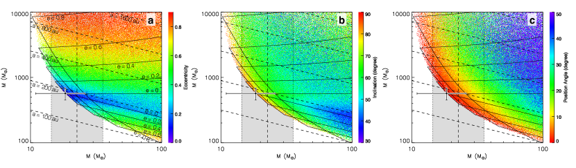
Supplementary Figure 1: The distribution of the possible binary properties in the space of system mass and orbital period. a: The color shows the eccentricity of the orbits. b: The color shows the inclination of the orbital plane relative to the plane of sky. c: The color shows the position angle of the intersection line between the orbital plane and the sky plane, with respect to the position angle of the line connecting Sources A and B. All possible elliptical orbits with eccentricities from 0 to 0.9 are considered. The data point and error bars correspond to the system mass, orbital period, and their $1\sigma$ uncertainties, assuming an edge-on circular orbit with the apparent separation of the two sources as their true separation. The dashed vertical line and the shaded regions indicate the system mass and its uncertainties derived from the free-free emissions. The dashed diagonal lines show the locations of orbits with different semi-major axes, as labelled in panel a. The solid lines encircle the regions for eccentricities of $e=0$, 0.2, 0.4, 0.6, and 0.8 (labelled in panel a).

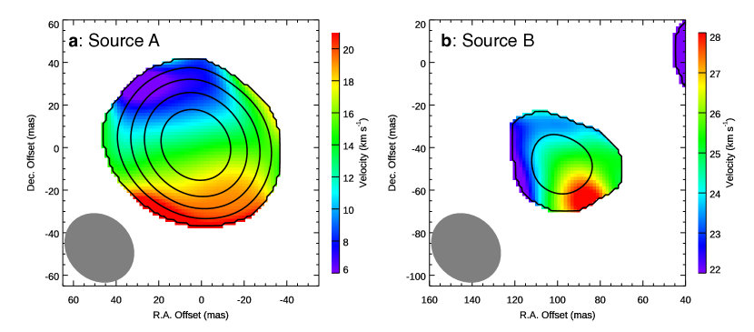
Supplementary Figure 2: The moment maps of the H30$\alpha$ emission in Source A (panel a) and B (panel b). The moment 0 maps (integrated emission) are shown in the black contours and the moment 1 maps (intensity-weighted mean velocities) are shown in the color scale. The moment 0 map in panel a is integrated in the velocity range of $-30~{}\mbox{km s}^{-1}<V_{\mathrm{lsr}}<55~{}\mbox{km s}^{-1}$, and the contour levels are $5\sigma\times 2^{n}$ ($n=1,2,3,...$) with $1\sigma=13~{}\mbox{mJy beam}^{-1}~{}\mbox{km s}^{-1}$. The moment 0 map in panel b is integrated in the velocity range of $-10~{}\mbox{km s}^{-1}<V_{\mathrm{lsr}}<60~{}\mbox{km s}^{-1}$, and the contour levels are $5\sigma\times 2^{n}$ ($n=1,2,3,...$) with $1\sigma=14~{}\mbox{mJy beam}^{-1}~{}\mbox{km s}^{-1}$. The synthesized beam is shown in the bottom-left corner.

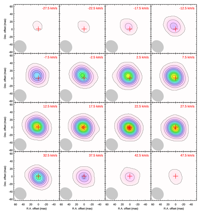
Supplementary Figure 3: The channel maps of the H30$\alpha$ emission in Source A. The channel width is $5~{}\mbox{km s}^{-1}$ and the central velocities of the channels are labeled in the upper-right corners of the panels. The contours start at 5$\sigma$ and have an interval of 10$\sigma$ with $1\sigma=17~{}\mbox{K}$ (0.8 $\mbox{mJy beam}^{-1}$). The synthesized beam is shown in the bottom-left corner of each panel. The red cross marks the position of the continuum peak.

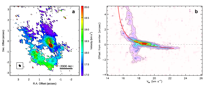
Supplementary Figure 4: The kinematics of the large scale CH₃OH emission. a: The moment maps of the large scale CH₃OH $4(2,2)-3(1,2)$ emission. The moment 0 map (emission integrated from $V_{\mathrm{lsr}}=15$ to $23~{}\mbox{km s}^{-1}$) is shown in the black contours and the moment 1 map (intensity-weighted mean velocities) is shown in the color scale. The contour levels start at 3$\sigma$ and have intervals of 6$\sigma$ ($1\sigma=7~{}\mbox{mJy beam}^{-1}~{}\mbox{km s}^{-1}$). The synthesized beam, shown inside the bottom-left square, is $0.25^{\prime\prime}\times 0.17^{\prime\prime}$. The red cross marks the position of the continuum peak. The dashed line indicates the cut for the position-velocity diagram shown in panel b. b: The position-velocity diagram of the CH₃OH emission along the cut shown in panel a. The cut width is $0.5^{\prime\prime}$. The contour levels start at 3$\sigma$ and have intervals of 3$\sigma$ ($1\sigma=4~{}\mbox{mJy beam}^{-1}$). The red curve is a model for explaining the kinematics (see Supplementary Discussion).

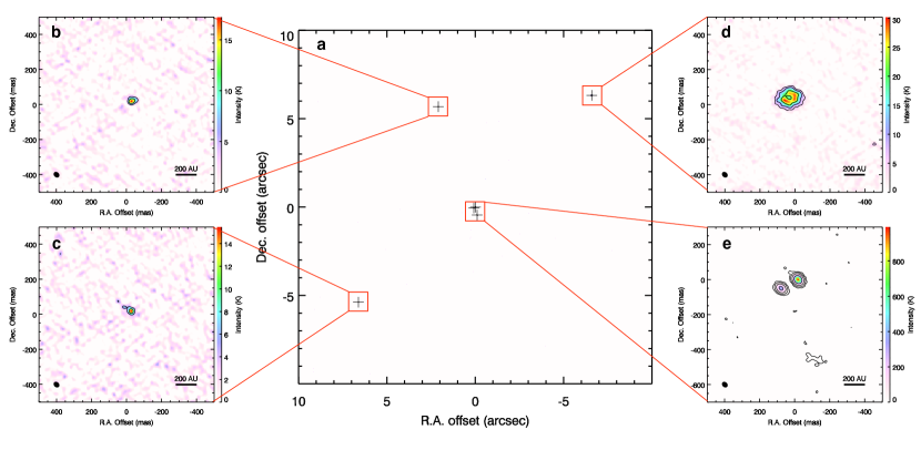
Supplementary Figure 5: Compact continuum sources identified in the high-resolution data. a: continuum map of the region $<10^{\prime\prime}$ from the central sources, with the crosses marking the identified continuum sources. b$-$e: Zoom-in views of the identified continuum sources.

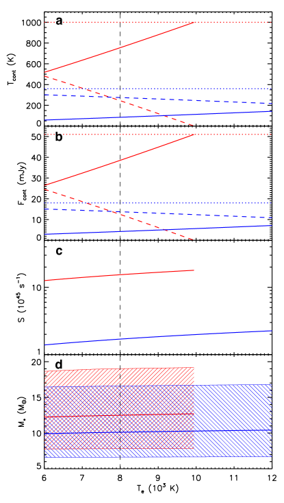
Supplementary Figure 6: Dependence of the estimated free-free peak intensities (panel a), fluxes (panel b), ionizing photon rates (panel c), and protostellar masses (panel d) of the two sources on the assumed ionized gas temperature. The red and blue colors are for Source A and B, respectively. The solid, dashed, and dotted lines in panels a and b are for the free-free, dust continuum, and total continuum emissions. The solid lines in panel d are estimated ZAMS stellar masses, and the shaded regions indicate the ranges of protostellar masses calculated from different accretion histories. The vertical line indicates the temperature of 8000 K of ionized gas, which is used as the fiducial case in the main text.

References

- [1] Chini, R., Hoffmeister, V. H., Nasseri, A., Stahl, O. & Zinnecker, H. A spectroscopic survey on the multiplicity of high-mass stars. Mon. Not. R. Astron. Soc. 424, 1925-1929 (2012).
- [2] Sana, H. et al. Binary interaction dominates the evolution of massive stars. Science 337, 444-446 (2012).
- [3] Peter, D., Feldt, M., Henning, Th. & Hormuth, F. Massive binaries in the Cepheus OB2/3 region. constraining the formation mechanism of massive stars. Astro. Astrophys. 538, A74 (2012).
- [4] Almeida, L. A. et al. The Tarantula massive binary monitoring: i. observational campaign and OB-type spectroscopic binaries. Astro. Astrophys. 598, A84 (2017).
- [5] Moe, M. & Di Stefano, R. Mind your Ps and Qs: the interrelation between period (P) and mass-ratio (Q) distributions of binary stars. Astrophys. J. Suppl. S. 230, 15 (2017).
- [6] Kratter, K. M., Matzner, C. D., Krumholz, M. R. & Klein, R. I. On the role of disks in the formation of stellar systems: a numerical parameter study of rapid accretion. Astrophys. J. 708, 1585-1597 (2010).
- [7] De Buizer, J. M. et al. The SOFIA massive (SOMA) star formation survey. i. overview and first results. Astrophys. J. 843, 33 (2017).
- [8] Reid, M. J. et al. Trigonometric parallaxes of massive star-forming regions. i. S252 & G232.6+1.0. Astrophys. J. 693, 397-405 (2009).
- [9] Tanaka, K., Tan, J. C. & Zhang, Y. Outflow-confined HII regions. i. first signposts of massive star formation. Astrophys. J. 818, 52 (2016).
- [10] Keto, E., Zhang, Q. & Kurtz, S. The early evolution of massive stars: radio recombination line spectra. Astrophys. J. 672, 423-432 (2008).
- [11] Keto, E. The formation of massive stars by accretion through trapped hypercompact HII regions. Astrophys. J. 599, 1196-1206 (2003).
- [12] Keto, E. & Wood, K. Observations on the formation of massive stars by accretion. Astrophys. J. 637, 850-859 (2006).
- [13] Guzmán, A. E. et al. The slow ionized wind and rotating disklike system that are associated with the high-mass young stellar object G345.4938+01.4677. Astrophys. J. 796, 117 (2014).
- [14] Zhang, Q., Claus, B., Watson, L. & Moran, J. Angular momentum in disk wind revealed in the young star MWC 349A. Astrophys. J. 837, 53 (2017).
- [15] Sakai, N. et al. Change in the chemical composition of infalling gas forming a disk around a protostar. Nature 507, 78-80 (2014).
- [16] Sridharan, T. K., Williams, S. J. & Fuller, G. A. The direct detection of a (proto)binary/disk system in IRAS 20126+4104. Astrophys. J. Lett. 631, L73-L76 (2005).
- [17] Beltrán, M. T. et al. Binary system and jet precession and expansion in G35.20-0.74N. Astro. Astrophys. 593, A49 (2016).
- [18] Beuther, H., Linz, H., Henning, Th., Feng, S. & Teague, R. Multiplicity and disks within the high-mass core NGC 7538IRS1. resolving cm line and continuum emission at resolution. Astro. Astrophys. 605, A61 (2017).
- [19] Kraus, S. et al. A high-mass protobinary system with spatially resolved circumstellar accretion disks and circumbinary disk. Astrophys. J. Lett. 835, L5 (2017).
- [20] McKee, C. F. & Tan, J. C. The formation of massive stars from turbulent cores. Astrophys. J. 585, 850-871 (2003).
- [21] Bonnell, I. A., Bate, M. R., Clarke, C. J. & Pringle, J. E. Competitive accretion in embedded stellar clusters. Mon. Not. R. Astron. Soc. 322, 785-794 (2001).
- [22] Myers, A. T., McKee, C. F., Cunningham, A. J., Klein, R. I. & Krumholz, M. R. The fragmentation of magnetized, massive star-forming cores with radiative feedback. Astrophys. J. 766, 97 (2013).
- [23] Takakuwa, S. et al. Spiral arms, infall, and misalignment of the circumbinary disk from the circumstellar disks in the protostellar binary system L1551 NE. Astrophys. J. 837, 86 (2017).

References

- [1] McMullin, J. P., Waters, B., Schiebel, D., Young, W. & Golap, K. CASA architecture and applications. ASP Conf. Ser. 376, 127-130 (2007).
- [2] Klaassen, P. D. et al. The evolution of young HII regions. i. continuum emission and internal dynamics. Astro. Astrophys. 611, A99 (2018).
- [3] Zhang, C.-P., Wang, J.-J., Xu, J.-L., Wyrowski, F. & Menten, K. M. Submillimeter array and very large array observations in the hypercompact HII region G35.58-0.03. Astrophys. J. 784, 107 (2014).
- [4] Araya, E. et al. A search for formaldehyde 6 cm emission toward young stellar objects. ii. H2CO and H110 observations. Astrophys. J. Suppl. S. 170, 152-174 (2007).
- [5] Liu, T., Wu, Y.-F. & Wang, K. A search for massive young stellar objects towards 98 CH3OH maser sources. Res. Astron. Astrophys. 10, 67-82 (2010).
- [6] Wilson, T. L., Rohlfs, K. & Hüttemeister, S. Tools of Radio Astronomy (Springer, 2013).
- [7] Shaver, P. A., McGee, R. X., Newton, L. M., Danks, A. C. & Pottasch, S. R. The galactic abundance gradient. Mon. Not. R. Astron. Soc. 204, 53-112 (1983).
- [8] Schmiedeke, A. et al. The physical and chemical structure of Sagittarius B2. i. three-dimensional thermal dust and free-free continuum modeling on 100 au to 45 pc scales. Astro. Astrophys. 588, A143 (2016).
- [9] Davies, B. et al. The Red MSX Source survey: critical tests of accretion models for the formation of massive stars. Mon. Not. R. Astron. Soc. 416, 972-990 (2011).
- [10] Meynet, G. & Maeder, A. Stellar evolution with rotation. v. changes in all the outputs of massive star models. Astro. Astrophys. 361, 101-120 (2000).
- [11] Lanz T. & Hubeny, I. A. Grid of NLTE line-blanketed model atmospheres of early B-type stars. Astrophys. J. Suppl. S. 169, 83-104 (2007).
- [12] Mottram, J. C. et al. The RMS survey: the luminosity functions and timescales of massive young stellar objects and compact HII regions. Astrophys. J. Lett. 730, L33 (2011).
- [13] Zhang, Y. & Tan, J. C. Radiation transfer of models of massive star formation. iv. the model grid and spectral energy distribution fitting. Astrophys. J. 853, 18 (2018).
- [14] Zhang, Y., Tan, J. C. & Hosokawa, T. Radiation transfer of models of massive star formation. iii. the evolutionary sequence. Astrophys. J. 788, 166 (2014).
- [15] Beltrán, M. T. et al. Accelerating infall and rotational spin-up in the hot molecular core G31.41+0.31. Astro. Astrophys. 615, A141 (2018).
- [16] Ossenkopf, V. & Henning, T. Dust opacities for protostellar cores. Astro. Astrophys. 291, 943-959 (1994).
- [17] Zhang, Y., Tan, J. C. & McKee, C. F. Radiation transfer of models of massive star formation. ii. effects of the outflow. Astrophys. J. 766, 86 (2013).
- [18] Condon, J. J. Errors in elliptical Gaussian fits. Publ. Astron. Soc. Pacific 109, 166-172 (1997).
- [19] Sánchez-Monge, Á. et al. A candidate circumbinary Keplerian disk in G35.20-0.74 N: a study with ALMA. Astro. Astrophys. 552, L10 (2013).
- [20] Ilee, J. D. et al. G11.92-0.61 MM1: a Keplerian disc around a massive young proto-O star. Mon. Not. R. Astron. Soc. 462, 4386-4401 (2016).

References

- [1] Sakai, N. et al. Change in the chemical composition of infalling gas forming a disk around a protostar. Nature 507, 78-80 (2014).
- [2] De Buizer, J. M. et al. The SOFIA massive (SOMA) star formation survey. i. overview and first results. Astrophys. J. 843, 33 (2017).
- [3] Krumholz, M. R., Klein, R. I. & McKee, C. F. Radiation-hydrodynamic simulations of collapse and fragmentation in massive protostellar cores. Astrophys. J. 656, 959-979 (2007)
- [4] Kratter, K. M., Matzner, C. D., Krumholz, M. R. & Klein, R. I. On the role of disks in the formation of stellar systems: a numerical parameter study of rapid accretion. Astrophys. J. 708, 1585-1597 (2010).