EV-IMO: Motion Segmentation Dataset
and Learning Pipeline for Event Cameras

Abstract

We present the first event-based learning approach for motion segmentation in indoor scenes and the first event-based dataset – EV-IMO – which includes accurate pixel-wise motion masks, egomotion and ground truth depth. Our approach is based on an efficient implementation of the SfM learning pipeline using a low parameter neural network architecture on event data. In addition to camera egomotion and a dense depth map, the network estimates independently moving object segmentation at the pixel-level and computes per-object 3D translational velocities of moving objects. We also train a shallow network with just 40k parameters, which is able to compute depth and egomotion.

Our EV-IMO dataset features 32 minutes of indoor recording with up to 3 fast moving objects in the camera field of view. The objects and the camera are tracked using a VICON^® motion capture system. By 3D scanning the room and the objects, ground truth of the depth map and pixel-wise object masks are obtained. We then train and evaluate our learning pipeline on EV-IMO and demonstrate that it is well suited for scene constrained robotics applications.

Supplementary Material

The supplementary video, code, trained models and appendix will be made available at http://prg.cs.umd.edu/EV-IMO.html.

The dataset is available at https://better-flow.github.io/evimo/.

I Introduction

In modern mobile robotics, autonomous agents are often found in unconstrained, highly dynamic environments, having to quickly navigate around humans or other moving robots. This renders the classical structure from motion (SfM) pipeline, often implemented via SLAM-like algorithms, not only inefficient but also incapable of solving the problem of navigation and obstacle avoidance. An autonomous mobile robot should be able to instantly detect every independently moving object in the scene, estimate the distance to it and predict its trajectory, while at the same time being aware of its own egomotion.

In this light, event-based processing has long been of interest to computational neuroscientists, and a new type of imaging device, known as “a silicon retina”, has been developed by the neuromorphic community. The event-based sensor does not record image frames, but asynchronous temporal changes in the scene in form of a continuous stream of events, each of which is generated when a given pixel detects a change in log light intensity. This allows the sensor to literally see the motion in the scene and makes it indispensable for motion processing and segmentation. The unique properties of event-based sensors - high dynamic range, high temporal resolution, low latency and high bandwidth allow these devices to function in the most challenging lighting conditions (such as almost complete darkness), while consuming a small amount of power.

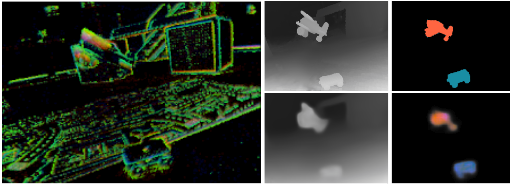
Figure 1: Depth and per-pixel pose inference on sparse event data, on our EV-IMO dataset. The top row is the ground truth depth and pose (the color corresponds to the objects’ linear velocities), the bottom row is the predicted network output. Camera egomotion is also estimated but not visualized here. Best viewed in color.

We believe that independent motion detection and estimation is an ideal application for event-based sensors, especially when applied to problems of autonomous robotics. Compared to classical cameras, event-based sensors encode spatio-temporal motion of image contours by producing a sparse data stream, which allows them to perceive extremely fast motion without experiencing motion blur. This, together with high tolerance to poor lighting conditions make this sensor a perfect fit for agile robots (such as quadrotors) which require a robust low latency visual pipeline.

On the algorithmic side, the estimation of 3D motion and scene geometry has been of great interest in Computer Vision and Robotics for quite a long time, but most works considered the scene to be static. Earlier classical algorithms studied the problem of Structure from Motion (SfM) [11] to develop “scene independent” constraints (e.g. the epipolar constraint [17] or depth positivity constraint [10]) and estimate 3D motion from images to facilitate subsequent scene reconstruction [12]. In recent years, most works have adopted the SLAM philosophy [8], where depth, 3D motion and image measurements are estimated together using iterative probabilistic algorithms. Such reconstruction approaches are known to be computationally heavy and often fail in the presence of outliers.

To move away from the restrictions imposed by the classical visual geometry approaches, the Computer Vision and Robotics community started to lean towards learning. Yet, while the problem of detecting moving objects has been studied both in the model-based and learning-based formulation, estimating object motion in addition to spatio-temporal scene reconstruction is still largely unexplored. An exception is the work in [36], which however does not provide an evaluation.

In this work we introduce a compositional neural network (NN) pipeline, which provides supervised up-to-scale depth and pixel-wise motion segmentation of the scene, as well as unsupervised 6 dof egomotion estimation and a per-segment linear velocity estimation using only monocular event data (see Fig. 1). This pipeline can be used in indoor scenarios for motion estimation and obstacle avoidance.

We also created a dataset, EV-IMO, which includes 32 minutes of indoor recording with multiple independently moving objects shot against a varying set of backgrounds and featuring different camera and object motions. To our knowledge, this is the first dataset for event-based cameras to include accurate pixel-wise masks of independently moving objects, apart from depth and trajectory ground truths.

To summarize, the contributions of this work are:

• The first NN for estimating both camera and object 3D motion using event data;

• The first dataset – EV-IMO – for motion segmentation with ground truth depth, per-object mask, camera and object motion;

• A novel loss function tailored for event alignment, measuring the profile sharpness of the motion compensated events;

• Demonstration of the feasibility of using a shallow low parameter multi-level feature NN architecture for event-based segmentation while retaining similar performance with the full-sized network.

II Related Work

II-A Event based Optical Flow, Depth and Motion Estimation

Many of the first event-based algorithms were concerned with optical flow. Different techniques employed the concepts of gradient computation [4, 1, 3, 25], template matching [22], and frequency computation [2, 6] on event surfaces. Zhu et al.  [45] proposed a self-supervised deep learning approach using the intensity signal from the DAVIS camera for supervision.

The problem of 3D motion estimation was studied following the visual odometry and SLAM formulation for the case of rotation only [28], with known maps [38, 7, 15], by combining event-based data with image measurements [21, 32], and using IMU sensors [44]. Other recent approaches jointly reconstruct the image intensity of the scene, and estimate 3D motion. First, in [19] only rotation was considered, and in [20] the general case was addressed.

II-B Independent Motion Detection

Many motion segmentation methods used in video applications are based on 2D measurements only [31, 26]. 3D approaches, such as the one here, model the camera’s rigid motion. Thompson and Pong [33] first suggested detecting moving objects by checking contradictions to the epipolar constraint. Vidal et al. [35] introduced the concept of subspace constraints for segmenting multiple objects. A good motion segmentation requires both constraints imposed by the camera motion and some form of scene constraints for clustering into regions. The latter can be achieved using approximate models of the rigid flow or the scene in view, for example by modeling the scene as planar, fitting multiple planes using the plane plus parallax constraint [18], or selecting models depending on the scene complexity [34]. In addition constraints on the occlusion regions [27] and discontinuities [14] have been used. Recently, machine learning techniques have been used for motion segmentation [13, 5]. As discussed next, the well-known SfM learner acquires both, the depth map and the rigid camera motion, and thus the flow due to rigid motion is fully constrained.

II-C Learning in Structure from Motion

In pioneering work, Saxena et al.  [30] demonstrated that shape can be learned from single images, inspiring many other supervised depth learning approaches (e.g. [9]). The concept was recently adopted in the SfM pipeline, and used in stereo [16] and video [39]. Most recently, Zhou et al.  [43] took it a step further, and showed how to estimate 3D motion and depth through the supervision of optical flow. Wang et al.  [37], instead of predicting depth in a separate network component, propose to incorporate a Direct Visual Odometry (DVO) pose predictor. Mahjourian et al.  [23] in addition to image alignment enforce alignment of the geometric scene structure in the loss function. Yang et al.  [40] added a 3D smoothness prior to the pipeline, which enables joint estimation of edges and 3D scene. Yin et al.  [42] include a non-rigid motion localization component to also detect moving objects. Our architecture is most closely related to SfM-Net [36], which learns using supervised and non-supervised components, depth, 3D camera and object motion. However, due to the lack of a dataset, the authors did not evaluate the object motion estimation. Finally, there are two related studies in the literature on event-based data: Zhu et al. [44] proposed the first unsupervised learning approach and applied it for optical flow estimation using the DAVIS sensor, where the supervision signal comes from the image component of the sensor. The arXiv paper [41] first adopted the full structure from motion pipeline. Different from our work, this paper, like [44], does not take advantage of the structure of event clouds. Most important, our work also detects, segments, and estimates the 3D motion of independently moving objects, and provides the means for evaluation.

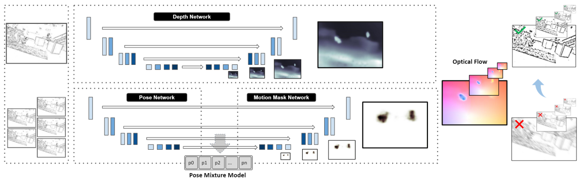
Figure 2: A depth network (top) uses an encoder-decoder architecture and is trained in supervised mode to estimate scene depth. A pose network (bottom left) takes consecutive event slices to generate a mixture model for the pixel-wise pose. A mixture of poses and mixture probabilities (bottom right) are outputs of this network. The outputs of the two networks are combined to generate the optical flow, then to inversely warp the inputs and backpropagate the error. Our networks utilize multi-level feature representations (shown in different darkness) for the underlying tasks.

III The Architecture

III-A Network Input

The raw data from the Dynamic Vision Sensor (DVS) is a continuous stream of events. Each event, $e(x,y,t,p)$ is encoded by its pixel position $(x,y)$, timestamp $t$, accurate to microseconds, and binary polarity, $p\in\{-1,1\}$, indicating whether the intensity of light decreased or increased.

In $(x,y,t)$ space, the event stream represents a 3D pointcloud. To leverage maximum information from this representation and pass it down to the network, we subdivide the event stream into consecutive time slices of size $\delta t$ (in our implementation - 25 $ms$). Every time slice is projected on a plane with a representation similar to our previous work [41] - we create a 3 channel map, with 2 channels being positive and negative event counts, and one channel being a timestamp aggregate, as first proposed in [24].

We then feed these 2D maps to the neural networks in our pipeline. The benefit of the 2D input representation is the reduction of data sparsity, and a resulting increase in efficiency compared to the 3D learning approaches. Yet, the 2D input may suffer from motion blur during fast motions. We tackle this problem by using a fine scale warping loss (sec. III-E1), which uses 1 $ms.$ slices to compute the loss.

III-B Overview of the Architecture

Our pipeline (see Fig. 2) consists of a depth prediction network and a pose prediction network. Both networks are low parameter [41] encoder-decoder networks [29]. Our depth network performs prediction on a single slice map. A supervision loss $Loss_{depth}$ comes by comparing with the ground truth as we describe in subsection III-E3. Our pose network uses up to 5 consecutive maps, to better account for the 3D structure of the raw event data. The pose network utilizes a mixture model to estimate pixel-wise 3D motion (relative pose) and corresponding motion masks from consecutive event slices. The masks are learned in supervised mode. We introduce a $Loss_{mask}$ on the motion mask. Finally, the two network outputs are used to generate the optical flow (Fig. 2, right). Successive event slices within a small period of time are then inversely warped. Perfectly motion compensated slices should stack into a sharp profile, and we introduce a two-stage $Loss_{warp}$ to measure the warping quality. The sum of the losses $Loss=Loss_{warp}+w_{depth}Loss_{depth}+w_{mask}Loss_{mask}$ is backpropagated to train flow, inverse depth, and pose.

III-C Ego-motion Model

We assume that the camera motion is rigid with a translational velocity $v=(v_{x},v_{y},v_{z})$ and a rotational velocity $\omega=(\omega_{x},\omega_{y},\omega_{z})$, and we also assume the camera to be calibrated. Let $\mathbf{X}=(X,Y,Z)^{T}$ be the world coordinates of a point and $\mathbf{x}=(x,y)^{T}$ be the corresponding image coordinates. The image velocity $\mathbf{u}=(u,v)^{T}$ is related to $\mathbf{x}$, the depth $Z$ and $t$ and $\omega$ as:

Thus, for each pixel, given the inverse depth, there is a linear relation between the optical flow and the 3D motion parameters (Eq. 1). As it is common in the literature, $\mathbf{p}$ denotes the 3D motion (or pose vector) $(\mathbf{v},\omega)^{T}$, and $A$ here denotes a $2\times 6$ matrix. Due to scaling ambiguity in this formulation, depth $Z$ and translation $(v_{x},v_{y},v_{z})$ are computed up to a scaling factor. In our practical implementation, we normalize $Z$ by the average depth.

We model the motion of individual moving objects as a 3D translation (without rotation), since most objects have relatively small size. The motion (pose) of any object is modeled as the sum of the rigid background motion and the object translation. Our network uses a mixture model for object segmentation - the 3D motion $p^{i}$ at a pixel $(x_{i},y_{i})$, is modeled as the sum of the camera motion $p_{ego}$ and weighted object translations, where the weights are obtained from motion masks as:

$$p^{i}=p_{ego}+\sum_{j=1}^{C}m_{j}^{i}t_{j},$$ (2)

In the above equation $m_{j}^{i}$ are the motion mask weights for the $i-th$ pixel and $t_{j}$ the estimated translations of the $C$ objects.

III-D A Mixture Model for Ego-motion and Independently Moving Objects

The pose network utilizes a mixture model to predict pixel-wise pose. The network output of the encoder part is a set of poses $(p_{0},t_{1},...,t_{C})$, where $p_{0}$ is the ego-motion pose $p_{ego}$, and $(t_{1},...,t_{C})$ are the translations with respect to the background or residual translations. The residual translations are added to the ego-motion pose as in Eq. 2 to get the candidate poses of objects relative to the camera.

In the decoding part, the network predicts pixel-wise mixture weights or motion masks for the poses. We use the mixture weights and the pose candidates to generate pixel-wise pose. The mixture weights sum to $1$ for each pixel. We found experimentally that allowing a pixel to belong to multiple rigid motions as opposed to only one, leads to better results. This is because soft assignment allows the model to explain more directions of motions. However, since during training, the object masks are provided, qualitatively sharp object boundaries are learned.

Using the mixture model representation allows us to differentiate object regions, moving with relatively small difference in 3D motion.

III-E Loss functions

We describe the loss functions used in the framework. It is noteworthy that the outputs of our networks are multi-scale. The loss functions described in this section are also calculated at various scales. They are weighted by the number of pixels and summed up to calculate the total loss.

III-E1 Event Warping Loss

In the training process, we calculate the optical flow and inversely warp events to compensate for the motion. This is done by measuring the warping loss at two time scales, first for a rough estimate, between slices, then for a refined estimate within a slice where we take full advantage of the timestamp information in the events.

Specifically, first using the optical flow estimate, we inversely warp neighboring slices to the center slice. To measure the alignment quality at the coarse scale, we take 3-5 consecutive event slices, where each consists of $25$ milliseconds of motion information, and we use the absolute difference in event counts after warping as the loss:

$$Loss_{coarse}=\sum_{-K\leq n\leq K,n\neq 0}|I^{warped}_{n}-I^{middle}|,$$

where $I^{warped}$ and $I^{middle}$ denote the three maps of positive events, negative events and average timestamps of the warped and the central slice, and $K$ is either 1 or 2. To refine the alignment, we process the event point clouds and divide the slices into smaller slices of $1ms$. Separately warping each of the small slices allows us to fully utilize the time information contained in the continuous event stream.

We stack warped slices and use the following sharpness loss to estimate the warping quality. Intuitively speaking, if the pose is perfectly estimated, the stacking of inversely warped slices should lead to a motion-deblurred sharp image. Let $S=\sum_{n=-N}^{N}|I^{warped}_{n}|$ be the stacking of inversely warped event slices, where $n$ represents the $n$-th slice in a stack of $2N+1$ slices. Our basic observation is that the sparse quasi-norm $||\cdot||_{p}$ for $0<p<1$ favors a sharp non-negative image over a blurred one. That is, $\sum_{i}|x_{i}|^{p}\geq(\sum_{i}|x_{i}|)^{p}$ for $0<p<1$. Based on this observation, we calculate the quasi-norm of $S$ to get the fine scale loss: $Loss_{fine}=||S||_{p},0<p<1$.

III-E2 Motion Mask Loss

Given the ground truth motion mask, we apply a binary cross entropy loss on the mixture weight of the ego-motion pose component to constrain that our model applies the ego-motion pose in the background region: $Loss_{mask}=-\sum_{i\in background}log(m_{0}^{i})$ To enforce that the mixture assignment is locally smooth, we also apply a smoothness loss on the first-order gradients of all the mixture weights.

III-E3 Depth Loss

With ground truth depth available, we enforce the depth network output to be consistent with the ground truth. We adjust the network output and the ground truth to the same scale, which we denote as $predict$ and $truth$ and apply the following penalty on their deviation: $Loss_{depth}=max(\frac{truth}{predict},\frac{predict}{truth})+\frac{|predict-truth|}{truth}$. Additionally, we apply a smoothness penalty on the second-order gradients of the prediction values, $Loss_{depth\_smooth}=||\Delta predict||_{1}$.

III-F Evenly Cascading Network Architecture

We adopt the low parameter evenly cascaded convolutional network (ECN) architecture as our backbone network design [41], and adapted it to an encoder decoder network borrowing concepts from the U-net design. The ECN network aggregates multilevel feature streams to make predictions. The low level features (Fig. 2, light blue blocks) are scaled with bilinear interpolation and improved throughout the whole encoding-decoding structure via residual learning. Along that, the network also progressively generates high level features (Fig. 2, darker blue blocks) in the encoding stage. The decoding stage proceeds reversely, the high level features are transformed by convolution and progressively merged back to the low level features to enhance them. Skip links (white arrows) are used in the network to connect features of the same shape, as in the original U-Net [29].

III-G Prediction of Depth and Component Weights

In the decoding stage, we make predictions using features at different resolutions and levels (Fig.  2). Initially, both high and low-level coarse features are used to predict a backbone prediction map. The prediction map is then upsampled and merged into existing feature maps for refinements in the remaining decoding layers. In the middle stage, high level features as well as features in the encoding layers are merged into the low level features to serve as modulation streams. The enhanced lower level features are used to estimate the prediction residue, which are usually also low-level structures. The residue is added to the current prediction map to refine it. The final prediction map is therefore obtained through successive upsamplings and refinements.

IV EV-IMO Dataset

One of the contributions of this work is the collection of the EV-IMO dataset - the first event camera dataset to include multiple independently moving objects and camera motion (at high speed), while providing accurate depth maps, per-object masks and trajectories at over 200 frames per second. The next sections describe our automated labeling pipeline, which allowed us to record more than 30 high quality sequences with a total length of half an hour. The source code for the dataset generation will be made available, to make it easier to expand the dataset in the future. A sample frame from the dataset is shown in Fig. 3.

IV-1 Methodology

Event cameras such as the DAVIS are designed to capture high speed motion and work in difficult lighting conditions. For such conditions classical methods of collecting depth ground truth, by calibrating a depth sensor with the camera, are extremely hard to apply - the motion blur from the fast motion would render such ground truth unreliable. Depth sensors have severe limitations in their frame rate as well. Furthermore it would be impossible to automatically acquire object masks - manual (or semi-automatic) annotation would be necessary. To circumvent these issues we designed a new approach:

1. A static high resolution 3D scan of the objects, as well as 3D room reconstruction is performed before the dataset recording takes place.

2. The VICON^® motion capture system is used to track both the objects and the camera during the recording.

3. The camera center as well as the object and room scans are calibrated with respect to the VICON^® coordinate frame.

4. For every pose update from the VICON motion capture, the 3D point clouds are transformed and projected on the camera plane, generating the per-pixel mask and ground truth depth.

This method allows to record accurate depth at very high frame rate, avoiding the problems induced by frame-based collection techniques. While we acknowledge that this approach requires expensive equipment, we argue that our method is superior for event-based sensors, since it allows to acquire the ground truth at virtually any event time stamp (by interpolating poses provided at 200 Hz) - a property impossible to achieve with manual annotation.

IV-2 Dataset Generation

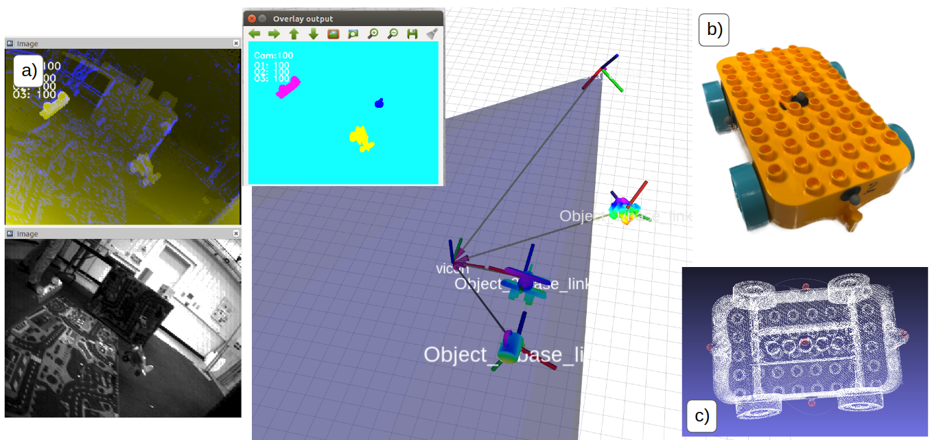
Figure 3: a) - The main interface of the automatic annotation tool. Camera cone of vision, depth and motion masks are visible. b) - Example object used in the dataset. c) 3D scan of the object.

Each of the candidate objects (up to 3 were recorded) were fitted with VICON^® motion capture reflective markers and 3D scanned using an industrial high quality 3D scanner. We use RANSAC to locate marker positions in the point cloud frame, and with the acquired point correspondences we transform the point cloud to the world frame at every update of the VICON. To scan the room, we place reflective markers on the Asus Xtion RGB-D sensor and use the tracking as an initialization for global ICP alignment.

To compute the position of the DAVIS camera center in the world frame we follow a simple calibration procedure, using a wand that is tracked by both VICON and camera. The calibration recordings will be provided with the dataset. The static pointcloud is then projected to the pixel coordinates $(x,y)$ in the camera center frame following equation 3:

$$(x,y,1)^{T}=KCP_{davis}^{-1}P_{cloud}X_{i}$$ (3)

Here, $K$ is the camera matrix, $P_{davis}$ is a $4\times 4$ transformation matrix between reflective markers on the DAVIS camera and the world, $C$ is the transformation between reflective markers on the DAVIS and the DAVIS camera center, $P_{cloud}$ is the transformation between markers in the 3D pointcloud and reflective markers in the world coordinate frame, and $X_{i}$ is the point in the 3D scan of the object.

Or dataset provides high resolution depth, pixel-wise object masks and accurate camera and object trajectories. We additionally compute, for every depth ground truth frame, the instantaneous camera velocity and the per-object velocity in the camera frame, which we use in our evaluations. We would like to mention, that our dataset allows to set varying ground truth frame rates - in all our experiments we generated ground truth at 40 frames per second.

IV-A Sequences

A short qualitative description of the sequences is given in Table I. We recorded 6 sets, each consisting of 3 to 19 sequences. The sets differ in the background (in both depth and the amount of texture), the number of moving objects, motion speeds, and lighting conditions.

A note on the dataset diversity: It is important to note, that for event-based cameras (which capture only edge information of the scene) the most important factor of diversity is the variability on motion. Different motions create 3D event clouds which vary significantly in their structure, even with similar backgrounds. Nevertheless, we organize our sequences into four background groups - ’table’, ’boxes’, ’plain wall’ and ’floor’ (see Fig 4), with the latter two having varying amounts of texture - an important factor for event cameras. We also include several tabletop scenes, with clutter and independently moving objects.

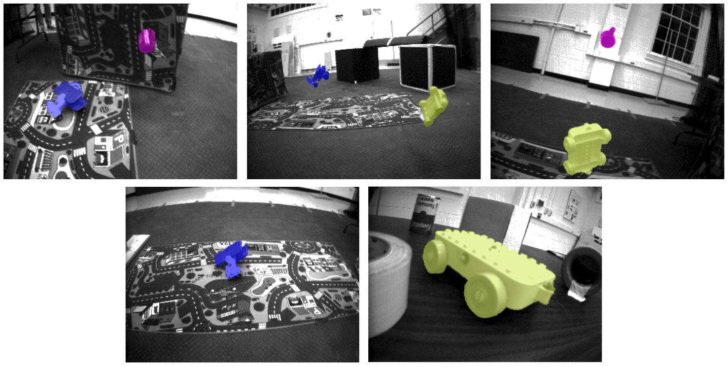
Figure 4: Types of background geometry featured in the EV-IMO dataset(from left to right): ’table’, ’boxes’, ’plain wall’, ’floor’ and ’tabletop’.

TABLE I: EV-IMO sequences

	background	speed	texture	occlusions	objects	light
Set 1	boxes	low	medium	low	1-2	normal
Set 2	floor/wall	low	low	low	1-3	normal
Set 3	table	high	high	medium	2-3	normal
Set 4	tabletop	low	high	high	1	normal
Set 5	tabletop	medium	high	high	2	normal
Set 6	boxes	high	medium	low	1-3	dark / flicker

V Experiments

Learning motion segmentation on event-based data is challenging because the data from event-based sensors is extremely sparse (coming only from object edges). Nevertheless, we were able to estimate the full camera egomotion, a dense depth map, and the 3D linear velocities of the independently moving objects in the scene.

We trained our networks with the Adam optimizer using a starting learning rate of $0.01$ with cosine annealing for 50 epochs. The batch size was 32. We distributed the training over $4$-Nvidia GTX 1080Ti GPUs and the training finished within 24 hours. Inference runs at over 100 fps on a single GTX 1080Ti.

In all experiments, we trained on ’box’ and ’floor’ backgrounds, and tested on ’table’ and ’plain wall’ backgrounds (see Table I and Fig. 4). For the Intersection over Union (IoU) scores, presented in Table II the inferenced object mask was thresholded at $0.5$.

Our baseline architecture contains approximately 2 million parameters. It has 32 initial hidden channels and a growth rate of 32. The feature scaling factors are $\frac{1}{2}$ and $2$ for the encoding and decoding. Overall the networks have 4 encoding and 4 decoding layers.

However, for many applications (such as autonomous robotics), precision is less important than computational efficiency and speed. We trained an additional shallow network with just 40 thousand parameters. In this setting we have 8 initial hidden channels and a growth rate of 8. The feature scaling factors are $\frac{1}{3}$ and $3$ respectively. The resulting networks have only 2 encoding and 2 decoding layers. We found that the 40k network is not capable of predicting object velocity reliably, but it produces reasonable camera egomotion, depth and motion masks, which can be tracked to extract the object translational velocities.

V-1 Qualitative Evaluation

Apart from the quantitative comparison we present a qualitative evaluation in Figs. 6 and 5. The per-object pose visualization (Fig. 6, columns 4 and 5) directly map the 3D linear velocity to RGB color space. The network is capable of predicting masks and pixel-wise pose in scenes with different amount of motion, number of objects or texture.

Fig. 5 shows how the quality of the depth and motion mask output is affected by reducing the size of the network. While the background depth is affected only to a small degree, the quality of the object mask and depth suffers notably.

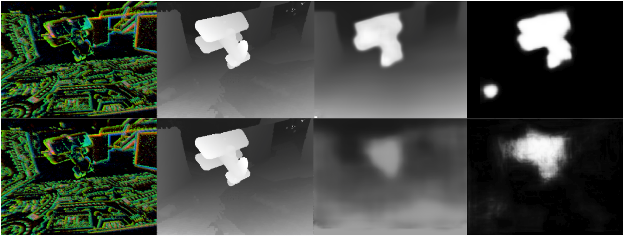
Figure 5: Comparison of the full network inference quality (2M parameters, top row) with the small version (40k parameters, bottom row)

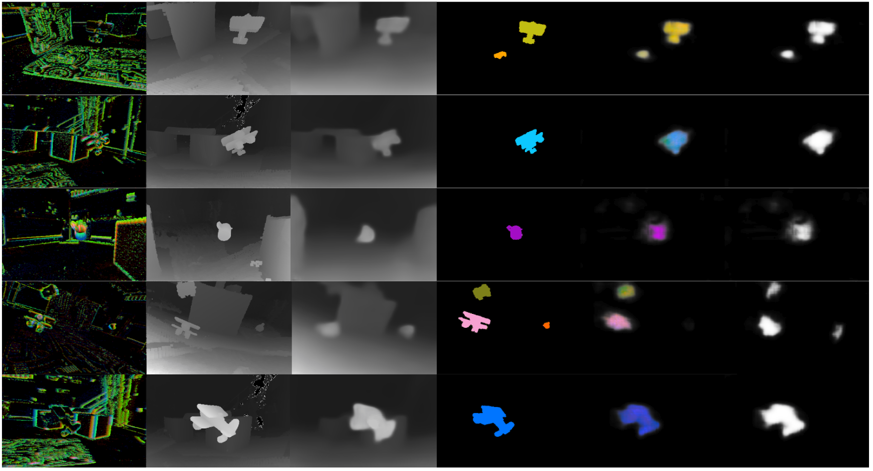
Figure 6: Qualitative results from our evaluation. The table entries from left to right: DVS input, ground truth for depth, network output for depth, ground truth pixel-wise pose, predicted pixel-wise pose, predicted motion mask. Examples were collected from EV-IMO dataset. Best viewed in color.

V-2 Segmentation and Motion Estimation

To evaluate the linear components of the velocities, for both egomotion and object motion, we compute the classical Average Endpoint Error (AEE). Since our pipeline is monocular, we apply the scale from the ground truth data in all our evaluations. To account for the rotational error of the camera (which does not need scaling) we compute the Average Relative Rotation Error $RRE=\|logm(R_{pred}^{T}R_{gt})\|_{2}$. Here $logm$ is the matrix logarithm, and $R$ are Euler rotation matrices. The $RRE$ essentially amounts to the total 3-dimensional angular rotation error of the camera. We also extract several sequences featuring fast camera motion and evaluate them separately. We present $AEE$ in m/s, and $RRE$ in radians/s in Table II.

We compute the averaged linear velocity of the independently moving objects within the object mask (since it is supplied by the network per pixel) and then also compute $AEE$. To evaluate the segmentation we compute the commonly used Intersection over Union (IoU) metric. Our results are presented in Table II.

TABLE II: Evaluation on segmentation and motion estimation. The numbers in braces are values for the 40k version of the network. $AEE$ is in m/s, $RRE$ is in rad/s.

	Cam $AEE$	Cam $RRE$	Obj AEE	IOU
$table$	0.07 (0.09)	0.05 (0.08)	0.19	0.83 (0.63)
$plainwall$	0.17 (0.23)	0.16 (0.24)	0.38	0.75 (0.58)
$fastmotion$	0.23 (0.28)	0.20 (0.26)	0.43	0.73 (0.59)

V-3 Comparison With Previous Work

As there is no public code available for monocular SfM on event-based data, we evaluate on a 4-parameter motion-compensation pipeline [24]. We evaluated the egomotion component of the network on a set of sequences without IMOs and with no roll/pitch egomotion and with planar background found in ’plain wall’ scenes, to make [24] applicable ([24] does not account for depth variation). Table  III reports the results in m/s for the translation and in rad/s for the rotation. We were not able to achieve any meaningful egomotion results on scenes with high depth variation for [24].

TABLE III: Comparison of $EV-IMO$ with  [24].

	$AEE$	$RRE$
EV-IMO	0.024	0.095
Classical [24]	0.031	0.134

We also evaluate our approach against a recent method [41] - ECN network, which estimates optical flow and depth on the event-based camera output. The method was originally designed and evaluated on a road driving sequence (which features a notably more simple and static environment, as well as significantly rudimentary egomotion). Still, we were able to tune [41] and train it on EV-IMO. We provide the comparison for the depth for our baseline method, the smaller version of our network (with just 40k parameters) and ECN in Table IV.

TABLE IV: Evaluation of the depth estimation

	Error metric			Accuracy metric
	Abs Rel	RMSE log	SILog	$\delta<1.25$	$\delta<1.25^{2}$	$\delta<1.25^{3}$
Baseline Approach
plain wall	0.16	0.26	0.07	0.87	0.95	0.97
cube background	0.13	0.20	0.04	0.87	0.97	0.99
table background	0.31	0.32	0.12	0.74	0.90	0.95
40k Network
plain wall	0.24	0.33	0.11	0.75	0.90	0.95
cube background	0.20	0.26	0.07	0.77	0.92	0.97
table background	0.33	0.34	0.15	0.65	0.87	0.95
ECN
plain wall	0.67	0.59	0.33	0.27	0.52	0.80
cube background	0.60	0.56	0.30	0.29	0.53	0.78
table background	0.47	0.48	0.23	0.45	0.69	0.86

We conducted the experiments on sequences featuring a variety of backgrounds and textures (the lack of texture is a limiting factor for event-based sensors). Even though ECN [41] was not designed to segment independently moving objects, the comparison is valid, since it infers depth from a single frame. Instead, we attribute the relatively low performance of [41] to a significantly more complex motion present in EV-IMO dataset, as well as more diverse depth background.

VI Conclusions

Event-based sensing promises advantages over classic video processing in applications of motion estimation because of the data’s unique properties of sparseness, high temporal resolution, and low latency. In this paper, we presented a compositional NN pipeline, which uses a combination of unsupervised and supervised components and is capable of generalizing well across different scenes. We also presented the first ever method of event-based motion segmentation with evaluation of both camera and object motion, which was achieved through the creation of a new state of the art indoor dataset - EV-IMO, recorded with the use of a VICON^® motion capture system.

Future work will delve into a number of issues regarding the design of the NN and usage of event data. Specifically, we consider it crucial to study event stream augmentation using partially or fully simulated data. We also plan to investigate ways to include tracking and connect the estimation over successive time slices, and investigate different alternatives of including the grouping of objects into the pipeline.

VII Acknowledgements

The support of the Northrop Grumman Mission Systems University Research Program, ONR under grant award N00014-17-1-2622, and the National Science Foundation under grant No. 1824198 are greatly acknowledged.

References

- [1] F. Barranco, C. Fermüller, and Y. Aloimonos. Contour motion estimation for asynchronous event-driven cameras. Proceedings of the IEEE, 102(10):1537–1556, 2014.
- [2] F. Barranco, C. Fermüller, and Y. Aloimonos. Bio-inspired motion estimation with event-driven sensors. In International Work-Conference on Artificial Neural Networks, pages 309–321. Springer, 2015.
- [3] R. Benosman, C. Clercq, X. Lagorce, S.-H. Ieng, and C. Bartolozzi. Event-based visual flow. IEEE Transactions on Neural Networks and Learning Systems, 25(2):407–417, 2014.
- [4] R. Benosman, S.-H. Ieng, C. Clercq, C. Bartolozzi, and M. Srinivasan. Asynchronous frameless event-based optical flow. Neural Netw., 27:32 – 37, Mar. 2012.
- [5] P. Bideau, A. RoyChowdhury, R. R. Menon, and E. Learned-Miller. The best of both worlds: combining cnns and geometric constraints for hierarchical motion segmentation. In Proceedings of the IEEE Conference on Computer Vision and Pattern Recognition, pages 508–517, 2018.
- [6] T. Brosch, S. Tschechne, and H. Neumann. On event-based optical flow detection. Frontiers in neuroscience, 9, 2015.
- [7] A. Censi, J. Strubel, C. Brandli, T. Delbruck, and D. Scaramuzza. Low-latency localization by active led markers tracking using a dynamic vision sensor. In IEEE/RSJ Int. Conf. onIntelligent Robots and Systems (IROS), pages 891–898. IEEE, 2013.
- [8] A. J. Davison, I. D. Reid, N. D. Molton, and O. Stasse. Monoslam: Real-time single camera slam. IEEE Transactions on Pattern Analysis & Machine Intelligence, 29(6):1052–1067, 2007.
- [9] D. Eigen, C. Puhrsch, and R. Fergus. Depth map prediction from a single image using a multi-scale deep network. In Advances in Neural Information Processing Systems, pages 2366–2374, 2014.
- [10] C. Fermüller. Passive navigation as a pattern recognition problem. International Journal of Computer Vision, 14(2):147–158, 1995.
- [11] C. Fermüller and Y. Aloimonos. Observability of 3d motion. International Journal of Computer Vision, 37(1):43–63, 2000.
- [12] C. Fermüller, L. Cheong, and Y. Aloimonos. Visual space distortion. Biological Cybernetics, 77(5):323–337, 1997.
- [13] K. Fragkiadaki, P. Arbelaez, P. Felsen, and J. Malik. Learning to segment moving objects in videos. In IEEE Conference on Computer Vision and Pattern Recognition (CVPR), June 2015.
- [14] K. Fragkiadaki, G. Zhang, and J. Shi. Video segmentation by tracing discontinuities in a trajectory embedding. In IEEE Conference on Computer Vision and Pattern Recognition, pages 1846–1853. IEEE, 2012.
- [15] G. Gallego, J. E. A. Lund, E. Mueggler, H. Rebecq, T. Delbrück, and D. Scaramuzza. Event-based, 6-dof camera tracking for high-speed applications. CoRR, abs/1607.03468, 2016.
- [16] R. Garg, V. K. BG, G. Carneiro, and I. Reid. Unsupervised cnn for single view depth estimation: Geometry to the rescue. In European Conference on Computer Vision, pages 740–756. Springer, 2016.
- [17] R. Hartley and A. Zisserman. Multiple View Geometry in Computer Vision. Cambridge University Press, 2003.
- [18] M. Irani and P. Anandan. A unified approach to moving object detection in 2d and 3d scenes. IEEE Transactions on Pattern Analysis and Machine Intelligence, 20(6):577–589, 1998.
- [19] H. Kim, A. Handa, R. Benosman, S.-H. Ieng, and A. J. Davison. Simultaneous mosaicing and tracking with an event camera. In British Machine Vision Conference, 2014.
- [20] H. Kim, S. Leutenegger, and A. J. Davison. Real-time 3d reconstruction and 6-dof tracking with an event camera. In European Conference on Computer Vision, pages 349–364. Springer, 2016.
- [21] B. Kueng, E. Mueggler, G. Gallego, and D. Scaramuzza. Low-latency visual odometry using event-based feature tracks. In IEEE/RSJ International Conference on Intelligent Robots and Systems (IROS), pages 16–23, 2016.
- [22] M. Liu and T. Delbruck. Block-matching optical flow for dynamic vision sensors: Algorithm and FPGA implementation. In IEEE International Symposium on Circuits and Systems (ISCAS), pages 1–4, 2017.
- [23] R. Mahjourian, M. Wicke, and A. Angelova. Unsupervised learning of depth and ego-motion from monocular video using 3d geometric constraints. CoRR, abs/1802.05522, 2018.
- [24] A. Mitrokhin, C. Fermüller, C. Parameshwara, and Y. Aloimonos. Event-based moving object detection and tracking. IEEE/RSJ Int. Conf. Intelligent Robots and Systems (IROS), 2018.
- [25] E. Mueggler, C. Forster, N. Baumli, G. Gallego, and D. Scaramuzza. Lifetime estimation of events from dynamic vision sensors. In IEEE International Conference on Robotics and Automation (ICRA) IEEE International Conference on, pages 4874–4881. IEEE, 2015.
- [26] J.-M. Odobez and P. Bouthemy. MRF-based motion segmentation exploiting a 2d motion model robust estimation. In Proc. International Conference on Image Processing, volume 3, pages 628–631. IEEE, 1995.
- [27] A. S. Ogale, C. Fermüller, and Y. Aloimonos. Motion segmentation using occlusions. IEEE Transactions on Pattern Analysis and Machine Intelligence, 27(6):988–992, 2005.
- [28] C. Reinbacher, G. Munda, and T. Pock. Real-time panoramic tracking for event cameras. arXiv preprint arXiv:1703.05161, 2017.
- [29] O. Ronneberger, P. Fischer, and T. Brox. U-net: Convolutional Networks for Biomedical Image Segmentation. In MICCAI (3), volume 9351 of Lecture Notes in Computer Science, pages 234–241. Springer, 2015.
- [30] A. Saxena, S. H. Chung, and A. Y. Ng. Learning depth from single monocular images. In Advances in Neural Information Processing Systems, pages 1161–1168, 2006.
- [31] D. Sun, E. B. Sudderth, and M. J. Black. Layered segmentation and optical flow estimation over time. In IEEE Conference on Computer Vision and Pattern Recognition, pages 1768–1775. IEEE, 2012.
- [32] D. Tedaldi, G. Gallego, E. Mueggler, and D. Scaramuzza. Feature detection and tracking with the dynamic and active-pixel vision sensor (DAVIS). In Second International Conference on Event-based Control, Communication, and Signal Processing (EBCCSP), pages 1–7, 2016.
- [33] W. B. Thompson and T.-C. Pong. Detecting moving objects. International Journal of Computer Vision, 4(1):39–57, Jan 1990.
- [34] P. H. Torr. Geometric motion segmentation and model selection. Philosophical Transactions of the Royal Society of London. Series A: Mathematical, Physical and Engineering Sciences, 356(1740):1321–1340, 1998.
- [35] R. Vidal, Y. Ma, and S. Sastry. Generalized principal component analysis (GPCA). In IEEE Computer Society Conference on Computer Vision and Pattern Recognition, 2003. Proceedings., volume 1, pages I–I, 2003.
- [36] S. Vijayanarasimhan, S. Ricco, C. Schmid, R. Sukthankar, and K. Fragkiadaki. Sfm-net: Learning of structure and motion from video, 2017.
- [37] C. Wang, J. M. Buenaposada, R. Zhu, and S. Lucey. Learning depth from monocular videos using direct methods. CoRR, abs/1712.00175, 2017.
- [38] D. Weikersdorfer, R. Hoffmann, and J. Conradt. Simultaneous localization and mapping for event-based vision systems. In International Conference on Computer Vision Systems, pages 133–142. Springer, 2013.
- [39] J. Xie, R. Girshick, and A. Farhadi. Deep3d: Fully automatic 2d-to-3d video conversion with deep convolutional neural networks. In European Conference on Computer Vision, pages 842–857. Springer, 2016.
- [40] Z. Yang, P. Wang, Y. Wang, W. Xu, and R. Nevatia. LEGO: learning edge with geometry all at once by watching videos. In Proc. IEEE Computer Vision and Pattern Recognition Conference, 2018.
- [41] C. Ye, A. Mitrokhin, C. Fermüller, J. A. Yorke, and Y. Aloimonos. Unsupervised learning of dense optical flow, depth and egomotion from sparse event data. CoRR, abs/1809.08625v2, 2018.
- [42] Z. Yin and J. Shi. Geonet: Unsupervised learning of dense depth, optical flow and camera pose. CoRR, abs/1803.02276, 2018.
- [43] T. Zhou, M. Brown, N. Snavely, and D. G. Lowe. Unsupervised learning of depth and ego-motion from video. In IEEE Conference on Computer Vision and Pattern Recognition (CVPR, 2017.
- [44] A. Z. Zhu, N. Atanasov, and K. Daniilidis. Event-based visual inertial odometry. In 2017 IEEE Conference on Computer Vision and Pattern Recognition (CVPR), pages 5816–5824, July 2017.
- [45] A. Z. Zhu, L. Yuan, K. Chaney, and K. Daniilidis. Ev-flownet: Self-supervised optical flow estimation for event-based cameras. Robotics: Science and Systems, 2018.