Ternary Syndrome Decoding with Large Weight

Abstract

The Syndrome Decoding problem is at the core of many code-based cryptosystems. In this paper, we study ternary Syndrome Decoding in large weight. This problem has been introduced in the Wave signature scheme but has never been thoroughly studied. We perform an algorithmic study of this problem which results in an update of the Wave parameters. On a more fundamental level, we show that ternary Syndrome Decoding with large weight is a really harder problem than the binary Syndrome Decoding problem, which could have several applications for the design of code-based cryptosystems.

Keywords.

Post-quantum cryptography, Syndrome Decoding problem, Subset Sum algorithms.

1 Introduction

Syndrome decoding is one of the oldest problems used in coding theory and cryptography [McE78]. It is known to be NP-complete [BMvT78] and its average case variant is still believed to be hard forty years after it was proposed, even against quantum computers. This makes code-based cryptography a credible candidate for post-quantum cryptography. There has been numerous proposals of post-quantum cryptosystems based on the hardness of the Syndrome Decoding (SD) problem, some of which were proposed for the NIST standardization process for quantum-resistant cryptographic schemes. Most of them are qualified for the second round of the competition [ABB⁺17, ACP⁺17, AMAB⁺17, BBC⁺19, BCL⁺17]. It is therefore a significant task to understand the computational hardness of the Syndrome Decoding problem.

Informally, the Syndrome Decoding problem is stated as follows. Given a matrix ${\mathbf{H}}\in\mathbb{F}_{q}^{(n-k)\times n}$, a vector ${\mathbf{s}}\in\mathbb{F}_{q}^{n-k}$ and a weight $w\in\llbracket 0,n\rrbracket$, the goal is to find a vector ${\mathbf{e}}\in\mathbb{F}_{q}^{n}$ such that ${\mathbf{H}}{{\mathbf{e}}}^{{\mathchoice{\raisebox{0.0pt}{$\displaystyle\intercal$}}{\raisebox{0.0pt}{$\textstyle\intercal$}}{\raisebox{0.0pt}{$\scriptstyle\intercal$}}{\raisebox{0.0pt}{$\scriptscriptstyle\intercal$}}}}={{\mathbf{s}}}^{{\mathchoice{\raisebox{0.0pt}{$\displaystyle\intercal$}}{\raisebox{0.0pt}{$\textstyle\intercal$}}{\raisebox{0.0pt}{$\scriptstyle\intercal$}}{\raisebox{0.0pt}{$\scriptscriptstyle\intercal$}}}}$ and $|{\mathbf{e}}|=w$, where $|{\mathbf{e}}|$ denotes the Hamming weight, namely $|{\mathbf{e}}|=|\{i:{\mathbf{e}}_{i}\neq 0\}|$. The binary case, i.e. when $q=2$ has been extensively studied. Even before this problem was used in cryptography, Prange [Pra62] constructed a clever algorithm for solving the binary problem using a method now referred to as Information Set Decoding (ISD).

1.1 Binary vs. Ternary Case

The binary case of the SD problem has been thoroughly studied. Its complexity is always studied for relative weight $W:=\frac{w}{n}\in[0,0.5]$ because the case $W>0.5$ is equivalent (see Remark 2 in Section 2). However, this argument is no longer valid in the general case ($q\geq 3$). Indeed, the large weight case does not behave similarly to the small weight case, as we can see on Figure 1.

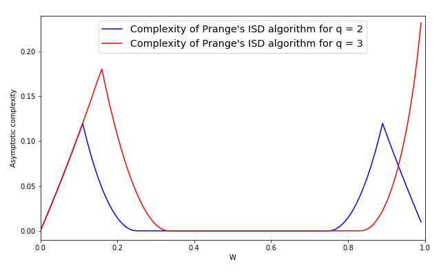
Figure 1: Asymptotic complexity of Prange’s ISD algorithm for $R:=\frac{k}{n}=0.5$.

The general case $q\geq 3$ has received much less attention than the binary case. One possible explanation for this is that there were no cryptographic applications for the general case. This has recently changed. Indeed, a new signature scheme named Wave was recently proposed in [DST18], based on the difficulty of SD on a ternary alphabet and with large weight. This scheme makes uses of the new regime of large weight induced by the asymmetry of the ternary case. Therefore, in addition to the algorithmic interest of studying the general syndrome decoding problem, the results of this study can be applied to a real cryptosystem.

Another reason why the general case $q\geq 3$ has been less studied is that the Hamming weight measure becomes less meaningful as $q$ grows larger. Indeed, the Hamming weight only counts the number of non-zero elements but not their repartition. Hence, the weight loses a significant amount of information for large values of $q$. Therefore, $q=3$ seems to be the best candidate to understand the structure of the non-binary case without losing too much information.

1.2 State of the Art for $q\geq 3$

Still, there exist some interesting results concerning the SD problem in the general $q$-ary case. Coffey and Goodman [CG90] were the firsts to propose a generalization of Prange’s ISD algorithm to $\mathbb{F}_{q}$. Following this seminal work, most existing ISD algorithms were extended to cover the $q$-ary case. In 2010, Peters [Pet10] generalized Stern’s algorithm. In his dissertation thesis, Meurer [Meu17] generalized the BJMM algorithm. Hirose [Hir16] proposed a generalization of Stern’s algorithm with May-Ozerov’s approach (using nearest neighbors) and showed that for $q\geq 3$ this does not improve the complexity compared to Stern’s classical approach. Later, Gueye, Klamti and Hirose [GKH17] extended the BJMM algorithm with May-Ozerov’s approach and improved the complexity of the general SD problem. A result from Canto-Torres [CT17] proves that all ISD-based algorithms converge to the same asymptotic complexity when $q\to\infty$. Finally, a recent work [IKR⁺18] proposed a generalization of the ball-collision decoding over $\mathbb{F}_{q}$.

All these papers focus solely on the SD problem for relative weight $W<0.5$. None of them mentions the case of large weight. The claimed worst case complexities in these papers should be understood as the worst case complexity for the SD problem with relative weight $W<0.5$, but as we can see on Figure 1 the highest complexity is actually reached for large relative weight.

1.3 Our Contributions

Our contribution consists in a general study of ternary syndrome decoding with large weight. We first focus on the Wave signature scheme [DST18] and present the best known algorithmic attack on this scheme. We then look more generally at the hardest instances of the ternary syndrome decoding with large weight and show that this problem seems significantly harder than the binary variant, making it a potentially very interesting problem for code-base cryptography.

The PGE+SS framework.

A first minor contribution consists in a modular description of most ISD-based algorithms. All these algorithms contain two steps. First, performing a partial Gaussian elimination (PGE), and then, solving a variant of the Subset Sum problem (SS). This was already implicitly used in previous papers but we want to make it explicit to simplify the analysis and hopefully make those algorithms easier to understand for non-specialists.

Ternary SD with large weight.

We then study specifically the SD problem in the ternary case and for large weights. From our modular description, we can focus only on finding many solutions of a specific instance of the Subset Sum problem. At a high level, we combine Wagner’s algorithm [Wag02] and representation techniques [BCJ11, BJMM12] to obtain our algorithm. Our first takeaway is that, while representations are very useful to obtain a unique solution (as in [BCJ11]), there are some drawbacks in using them to obtain many solutions. These drawbacks are strongly mitigated in the binary case as in [BJMM12] but it becomes much harder for larger values of $q$. We manage to partially compensate this by changing the moduli size, the place and the number of representations. For instance, for the Wave [DST18] parameters, we derive an algorithm that is a Wagner tree with seven floors where the last two floors have partial representations and the others have none.

New parameters for Wave.

We then use our algorithms to study the complexity of the Wave signature scheme, for which we significantly improve the original analysis. We show that the key sizes of the original scheme presented for 128 bits of security have to be more than doubled, going roughly from 1Mb to 2.2Mb, to achieve the claimed security. This requires to study the Decode One Out of Many (DOOM) problem, on which Wave actually relies. This problem corresponds to a multiple target SD problem. More precisely, given $N$ syndromes $({\mathbf{s}}_{1},\ldots,{\mathbf{s}}_{N})$ ($N$ can be large, for example $N=2^{64}$) the goal is to find an error ${\mathbf{e}}$ of Hamming weight $w$ and an integer $i$ such that ${\mathbf{e}}{{\mathbf{H}}}^{{\mathchoice{\raisebox{0.0pt}{$\displaystyle\intercal$}}{\raisebox{0.0pt}{$\textstyle\intercal$}}{\raisebox{0.0pt}{$\scriptstyle\intercal$}}{\raisebox{0.0pt}{$\scriptscriptstyle\intercal$}}}}={\mathbf{s}}_{i}$.

Hardest instances of the ternary SD with large weight.

Next, we look at the hardest instances of the ternary SD with large weight problem. We study the standard ISD algorithms and show that for all of them, the hardest instances occur for $R\approx 0.369$ and $W=1$ (still in the case $q=3$). Unsurprisingly, for equivalent code length and dimension, ternary syndrome decoding is harder than its binary counterpart. But this is due to the fact that the input matrix contains more information, since its elements are in $\mathbb{F}_{3}$, hence the input size is $\log_{2}(3)$ times larger than a binary matrix with equivalent dimensions.

A more surprising conclusion of our work is that ternary syndrome decoding is significantly harder than the binary case for equivalent input size, that is, when normalizing the exponent by a factor $\log_{2}(q)$. This new result is in sharp contrast with all the previous work on $q$-ary syndrome decoding that showed that the problem becomes simpler as $q$ increases. This is due to the fact that all the previous literature only considered the small weight case while we now take large weights into account.

Table 1 represents the minimum input size for which the underlying syndrome decoding problem offers $128$ bits of security, i.e. the associated algorithm needs at least $2^{128}$ operations to solve the problem.

Algorithm	$q=2$	$q=3$ and $W>0.5$
Prange	275	44
Dumer/Wagner	295	83
BJMM/Our algorithm	374	99

Table 1: Minimum input sizes (in kbits) for a time complexity of $2^{128}$.

We want to stress again that those input sizes in the ternary case take into account the fact that the matrix elements are in $\mathbb{F}_{3}$. So the increase in efficiency is quite significant and the ternary SD could efficiently replace its binary counterpart when looking for a hard code-based problem.

1.4 Notations

We define here some notations that will be used throughout the paper. The notation $x\mathop{=}\limits^{\triangle}y$ means that $x$ is defined to be equal to $y$. We denote by $\mathbb{F}_{q}=\{0,1,\cdots,q-1\}$ the finite field of size $q$. Vectors will be written with bold letters (such as ${\mathbf{e}}$) and uppercase bold letters will be used to denote matrices (such as ${\mathbf{H}}$). Vectors are in row notation. Let ${\mathbf{x}}$ and ${\mathbf{y}}$ be two vectors, we will write $({\mathbf{x}},{\mathbf{y}})$ to denote their concatenation. Finally, we denote by $\llbracket a,b\rrbracket$ the set $\{\tilde{a},\tilde{a}+1,\dots,\tilde{b}\}$ where $\tilde{a}=\lfloor a\rfloor$ and $\tilde{b}=\lfloor b\rfloor$.

2 A General Framework for Solving the Syndrome Decoding Problem

2.1 The Syndrome Decoding Problem

The goal of this paper is to study the Syndrome Decoding problem, which is at the core of most code-based cryptosystems.

Problem 1 ()

[Syndrome Decoding - $\mathrm{SD}(q,R,W)$]

Instance:	${\mathbf{H}}\in\mathbb{F}_{q}^{(n-k)\times n}$ of full rank,
	${\mathbf{s}}\in\mathbb{F}_{q}^{n-k}$ (usually called the syndrome).
Output:	${\mathbf{e}}\in\mathbb{F}_{q}^{n}$ such that $|{\mathbf{e}}|=w$ and ${\mathbf{e}}{{\mathbf{H}}}^{{\mathchoice{\raisebox{0.0pt}{$\displaystyle\intercal$}}{\raisebox{0.0pt}{$\textstyle\intercal$}}{\raisebox{0.0pt}{$\scriptstyle\intercal$}}{\raisebox{0.0pt}{$\scriptscriptstyle\intercal$}}}}={\mathbf{s}}$,

  

where $k\mathop{=}\limits^{\triangle}\lceil Rn\rceil$, $w\mathop{=}\limits^{\triangle}\lceil Wn\rceil$ and $|{\mathbf{e}}|\mathop{=}\limits^{\triangle}|\{i:{\mathbf{e}}_{i}\neq 0\}|$.

The problem $\mathrm{SD}(q,R,W)$ is parametrized by the field size $q$, the rate $R\in[0,1]$ and the relative weight $W\in[0,1]$. We are always interested in the average case complexity (as a function of $n$) of this problem, where ${\mathbf{H}}$ is chosen uniformly at random and ${\mathbf{s}}$ is chosen uniformly from the set $\{{\mathbf{e}}{{\mathbf{H}}}^{{\mathchoice{\raisebox{0.0pt}{$\displaystyle\intercal$}}{\raisebox{0.0pt}{$\textstyle\intercal$}}{\raisebox{0.0pt}{$\scriptstyle\intercal$}}{\raisebox{0.0pt}{$\scriptscriptstyle\intercal$}}}}:|{\mathbf{e}}|=w\}$. This ensures the existence of a solution for each input and corresponds to the typical situation in cryptanalysis. More generally, the following proposition gives the average expected number of solutions

Proposition 1

Let $n,k,w$ be integers with $k\leq n$ and ${\mathbf{s}}\in\mathbb{F}_{q}^{n-k}$. The expected number of solutions of ${\mathbf{e}}{{\mathbf{H}}}^{{\mathchoice{\raisebox{0.0pt}{$\displaystyle\intercal$}}{\raisebox{0.0pt}{$\textstyle\intercal$}}{\raisebox{0.0pt}{$\scriptstyle\intercal$}}{\raisebox{0.0pt}{$\scriptscriptstyle\intercal$}}}}={{\mathbf{s}}}$ in ${\mathbf{e}}$ of weight $w$ when ${\mathbf{H}}$ is chosen uniformly at random in $\mathbb{F}_{q}^{(n-k)\times n}$ is given by:

$$\frac{\binom{n}{w}(q-1)^{w}}{q^{n-k}}.$$

Proof

This is simple combinatorics. The numerator corresponds to the number of vectors ${\mathbf{e}}^{\prime}$ of weight $w$. The denominator corresponds to the inverse of the probability over ${\mathbf{H}}$ that ${\mathbf{e}}{{\mathbf{H}}}^{{\mathchoice{\raisebox{0.0pt}{$\displaystyle\intercal$}}{\raisebox{0.0pt}{$\textstyle\intercal$}}{\raisebox{0.0pt}{$\scriptstyle\intercal$}}{\raisebox{0.0pt}{$\scriptscriptstyle\intercal$}}}}={{\mathbf{s}}}^{{\mathchoice{\raisebox{0.0pt}{$\displaystyle\intercal$}}{\raisebox{0.0pt}{$\textstyle\intercal$}}{\raisebox{0.0pt}{$\scriptstyle\intercal$}}{\raisebox{0.0pt}{$\scriptscriptstyle\intercal$}}}}$ for ${\mathbf{e}}\neq\mathbf{0}$. ∎

Remark 1

The matrix length $n$ is not considered as a parameter of the problem since we are only interested in the asymptopic complexity, that is the coefficient $F(q,R,W)$ (which does not depend on $n$) such that the complexity of the Syndrome Decoding problem for a matrix of size $n$ can be expressed as $2^{n(F(q,R,W)+o(1))}$.

2.1.1 State of the Art on $\mathbb{F}_{2}$.

This problem was mostly studied in the case $q=2$. Depending on the parameters $R$ and $W$, the complexity of the problem can greatly vary. Let us fix a value $R$, and let $W_{\textup{GV}}$ denote the Gilbert-Varshamov bound, that is $W_{\textup{GV}}\mathop{=}\limits^{\triangle}h_{2}^{-1}(1-R)$ where $h_{2}$ is the binary entropy function restricted to the input space $\left[0,\frac{1}{2}\right]$. For $W\in\left[0,\frac{1}{2}\right]$, there exist three different regimes.

1. $W\approx W_{\textup{GV}}$. When $W$ is close to $W_{\textup{GV}}$, there is on average a small number of solutions. This is the regime where the problem is the hardest and where it is the most studied. To the best of our knowledge, we only know two code-based cryptosystems in this regime, namely the CFS signature scheme [CFS01] and the authentication scheme of Stern [Ste93].

2. $W\gg W_{\textup{GV}}$. In this case, there are on average exponentially many solutions and this makes the problem simpler. When $W$ reaches $\frac{1-R}{2}$, the problem can be solved in average polynomial time using Prange’s algorithm [Pra62]. There is a cryptographic motivation to consider $W$ much larger than $W_{\textup{GV}}$, for instance to build signatures schemes following the [GPV08] paradigm as it was done in [DST17] but one has to be careful to not make $\mathrm{SD}$ too simple.

3. $W\ll W_{\textup{GV}}$. In this regime, we have with high probability a unique solution. However, the search space, i.e. the set of vectors ${\mathbf{e}}$ st. $|{\mathbf{e}}|=\lceil Wn\rceil$ is much smaller than in the other regimes. The original McEliece system [McE78] or the QC-MDPC systems [MTSB12] are in this regime.

Remark 2

Solving $\mathrm{SD}(2,R,W)$ for $W\in\left[\frac{1}{2},1\right]$ and the instance $({\mathbf{H}},{\mathbf{s}})$ can be reduced to one of the above-mentioned cases using $\mathrm{SD}(2,R,1-W)$ and the instance $({\mathbf{H}},{\mathbf{s}}+\mathbf{1}{{\mathbf{H}}}^{{\mathchoice{\raisebox{0.0pt}{$\displaystyle\intercal$}}{\raisebox{0.0pt}{$\textstyle\intercal$}}{\raisebox{0.0pt}{$\scriptstyle\intercal$}}{\raisebox{0.0pt}{$\scriptscriptstyle\intercal$}}}})$ where $\mathbf{1}$ denotes the vector with all its components equal to $1$.

Remark 3

Contrary to the binary case, when $q\geq 3$ the case of large relative weight can not be reduced to that of small relative weight using the trick of Remark 2. In fact, the problem has a quite different behavior in small and large weights, see Figure 1.

2.2 The PGE+SS Framework in $\mathbb{F}_{q}$

The $\mathrm{SD}$ problem has been extensively studied in the binary case. Most algorithms designed to solve this problem [Dum91, MMT11, BJMM12] follow the same framework:

1. perform a partial Gaussian elimination (PGE) ;

2. solve the Subset Sum problem (SS) on a reduced instance.

We will see how we can extend this framework to the non-binary case. Our goal here is to describe the PGE+SS framework for solving $\mathrm{SD}(q,R,W)$. Fix ${\mathbf{H}}\in\mathbb{F}_{q}^{(n-k)\times n}$ of full rank and ${\mathbf{s}}\in\mathbb{F}_{q}^{n-k}$. Recall that we want to find ${\mathbf{e}}\in\mathbb{F}_{q}^{n}$ such that $|{\mathbf{e}}|=w\mathop{=}\limits^{\triangle}\ \lceil Wn\rceil$ and ${\mathbf{H}}{{\mathbf{e}}}^{{\mathchoice{\raisebox{0.0pt}{$\displaystyle\intercal$}}{\raisebox{0.0pt}{$\textstyle\intercal$}}{\raisebox{0.0pt}{$\scriptstyle\intercal$}}{\raisebox{0.0pt}{$\scriptscriptstyle\intercal$}}}}={{\mathbf{s}}}^{{\mathchoice{\raisebox{0.0pt}{$\displaystyle\intercal$}}{\raisebox{0.0pt}{$\textstyle\intercal$}}{\raisebox{0.0pt}{$\scriptstyle\intercal$}}{\raisebox{0.0pt}{$\scriptscriptstyle\intercal$}}}}$. Let us introduce $\ell$ and $p$, two parameters of the system, that we will consider fixed for now. In this framework, an algorithm for solving $\mathrm{SD}(q,R,W)$ will consist of $4$ steps: a permutation step, a partial Gaussian Elimination step, a Subset Sum step and a test step.

1. Permutation step. Pick a random permutation $\pi$. Let ${\mathbf{H}_{\pi}}$ be the matrix ${\mathbf{H}}$ where the columns have been permuted according to $\pi$. We now want to solve the problem $\mathrm{SD}(q,R,W)$ on inputs ${\mathbf{H}_{\pi}}$ and ${\mathbf{s}}$.

2. Partial Gaussian Elimination step. If the top left square submatrix of ${\mathbf{H}_{\pi}}$ of size $n-k-\ell$ is not of full rank, go back to step $1$ and choose another random permutation $\pi$. This happens with constant probability. Else, if this submatrix is of full rank, perform a Gaussian elimination on the rows of ${\mathbf{H}_{\pi}}$ using the first $n-k-\ell$ columns. Let ${\mathbf{S}}\in\mathbb{F}_{q}^{(n-k)\times(n-k)}$ be the invertible matrix corresponding to this operation. We now have two matrices ${\mathbf{H}}^{\prime}\in\mathbb{F}_{q}^{(n-k-\ell)\times(k+\ell)}$ and ${\mathbf{H}}^{\prime\prime}\in\mathbb{F}_{q}^{\ell\times(k+\ell)}$ such that:

   $${\mathbf{S}}{\mathbf{H}_{\pi}}=\begin{pmatrix}{\boldsymbol{1}}_{n-k-\ell}&{\mathbf{H}}^{\prime}\\ \mathbf{0}&{\mathbf{H}}^{\prime\prime}\end{pmatrix}.$$

   The error ${\mathbf{e}}$ can be written as ${\mathbf{e}}=({\mathbf{e}}^{\prime},{\mathbf{e}}^{\prime\prime})$ where ${\mathbf{e}}^{\prime}\in\mathbb{F}_{q}^{n-k-\ell}$ and ${\mathbf{e}}^{\prime\prime}\in\mathbb{F}_{q}^{k+\ell}$, and one can write ${\mathbf{s}}{{\mathbf{S}}}^{{\mathchoice{\raisebox{0.0pt}{$\displaystyle\intercal$}}{\raisebox{0.0pt}{$\textstyle\intercal$}}{\raisebox{0.0pt}{$\scriptstyle\intercal$}}{\raisebox{0.0pt}{$\scriptscriptstyle\intercal$}}}}=({\mathbf{s}}^{\prime},{\mathbf{s}}^{\prime\prime})$ with ${\mathbf{s}}^{\prime}\in\mathbb{F}_{q}^{n-k-\ell}$ and ${\mathbf{s}}^{\prime\prime}\in\mathbb{F}_{q}^{\ell}$.

   $${\mathbf{H}_{\pi}}{{\mathbf{e}}}^{{\mathchoice{\raisebox{0.0pt}{$\displaystyle\intercal$}}{\raisebox{0.0pt}{$\textstyle\intercal$}}{\raisebox{0.0pt}{$\scriptstyle\intercal$}}{\raisebox{0.0pt}{$\scriptscriptstyle\intercal$}}}}={{\mathbf{s}}}^{{\mathchoice{\raisebox{0.0pt}{$\displaystyle\intercal$}}{\raisebox{0.0pt}{$\textstyle\intercal$}}{\raisebox{0.0pt}{$\scriptstyle\intercal$}}{\raisebox{0.0pt}{$\scriptscriptstyle\intercal$}}}} \iff{\mathbf{S}}{\mathbf{H}}_{\pi}{{\mathbf{e}}}^{{\mathchoice{\raisebox{0.0pt}{$\displaystyle\intercal$}}{\raisebox{0.0pt}{$\textstyle\intercal$}}{\raisebox{0.0pt}{$\scriptstyle\intercal$}}{\raisebox{0.0pt}{$\scriptscriptstyle\intercal$}}}}={\mathbf{S}}{{\mathbf{s}}}^{{\mathchoice{\raisebox{0.0pt}{$\displaystyle\intercal$}}{\raisebox{0.0pt}{$\textstyle\intercal$}}{\raisebox{0.0pt}{$\scriptstyle\intercal$}}{\raisebox{0.0pt}{$\scriptscriptstyle\intercal$}}}}$$

   $$\iff\begin{pmatrix}{\boldsymbol{1}}_{n-k-\ell}&{\mathbf{H}}^{\prime}\\ \mathbf{0}&{\mathbf{H}}^{\prime\prime}\end{pmatrix}\begin{pmatrix}{{\mathbf{e}}^{\prime}}^{{\mathchoice{\raisebox{0.0pt}{$\displaystyle\intercal$}}{\raisebox{0.0pt}{$\textstyle\intercal$}}{\raisebox{0.0pt}{$\scriptstyle\intercal$}}{\raisebox{0.0pt}{$\scriptscriptstyle\intercal$}}}}\\ {{\mathbf{e}}^{\prime\prime}}^{{\mathchoice{\raisebox{0.0pt}{$\displaystyle\intercal$}}{\raisebox{0.0pt}{$\textstyle\intercal$}}{\raisebox{0.0pt}{$\scriptstyle\intercal$}}{\raisebox{0.0pt}{$\scriptscriptstyle\intercal$}}}}\end{pmatrix}=\begin{pmatrix}{{\mathbf{s}}^{\prime}}^{{\mathchoice{\raisebox{0.0pt}{$\displaystyle\intercal$}}{\raisebox{0.0pt}{$\textstyle\intercal$}}{\raisebox{0.0pt}{$\scriptstyle\intercal$}}{\raisebox{0.0pt}{$\scriptscriptstyle\intercal$}}}}\\ {{\mathbf{s}}^{\prime\prime}}^{{\mathchoice{\raisebox{0.0pt}{$\displaystyle\intercal$}}{\raisebox{0.0pt}{$\textstyle\intercal$}}{\raisebox{0.0pt}{$\scriptstyle\intercal$}}{\raisebox{0.0pt}{$\scriptscriptstyle\intercal$}}}}\end{pmatrix}$$

   $$\iff\left\{\begin{array}[]{ll}{{\mathbf{e}}^{\prime}}^{{\mathchoice{\raisebox{0.0pt}{$\displaystyle\intercal$}}{\raisebox{0.0pt}{$\textstyle\intercal$}}{\raisebox{0.0pt}{$\scriptstyle\intercal$}}{\raisebox{0.0pt}{$\scriptscriptstyle\intercal$}}}}+{\mathbf{H}}^{\prime}{{\mathbf{e}}^{\prime\prime}}^{{\mathchoice{\raisebox{0.0pt}{$\displaystyle\intercal$}}{\raisebox{0.0pt}{$\textstyle\intercal$}}{\raisebox{0.0pt}{$\scriptstyle\intercal$}}{\raisebox{0.0pt}{$\scriptscriptstyle\intercal$}}}}={{\mathbf{s}}^{\prime}}^{{\mathchoice{\raisebox{0.0pt}{$\displaystyle\intercal$}}{\raisebox{0.0pt}{$\textstyle\intercal$}}{\raisebox{0.0pt}{$\scriptstyle\intercal$}}{\raisebox{0.0pt}{$\scriptscriptstyle\intercal$}}}}\\ {\mathbf{H}}^{\prime\prime}{{\mathbf{e}}^{\prime\prime}}^{{\mathchoice{\raisebox{0.0pt}{$\displaystyle\intercal$}}{\raisebox{0.0pt}{$\textstyle\intercal$}}{\raisebox{0.0pt}{$\scriptstyle\intercal$}}{\raisebox{0.0pt}{$\scriptscriptstyle\intercal$}}}}={{\mathbf{s}}^{\prime\prime}}^{{\mathchoice{\raisebox{0.0pt}{$\displaystyle\intercal$}}{\raisebox{0.0pt}{$\textstyle\intercal$}}{\raisebox{0.0pt}{$\scriptstyle\intercal$}}{\raisebox{0.0pt}{$\scriptscriptstyle\intercal$}}}}\end{array}\right.$$ (1)

   To solve the problem, we will try to find a solution $({\mathbf{e}}^{\prime},{\mathbf{e}}^{\prime\prime})$ to the above system such that $|{\mathbf{e}}^{\prime\prime}|=p$ and $|{\mathbf{e}}^{\prime}|=w-p$.

3. The Subset Sum step. Compute a set $\mathcal{S}\subseteq\mathbb{F}_{q}^{k+\ell}$ of solutions ${\mathbf{e}}^{\prime\prime}$ of ${\mathbf{H}}^{\prime\prime}{{\mathbf{e}}^{\prime\prime}}^{{\mathchoice{\raisebox{0.0pt}{$\displaystyle\intercal$}}{\raisebox{0.0pt}{$\textstyle\intercal$}}{\raisebox{0.0pt}{$\scriptstyle\intercal$}}{\raisebox{0.0pt}{$\scriptscriptstyle\intercal$}}}}={{\mathbf{s}}^{\prime\prime}}^{{\mathchoice{\raisebox{0.0pt}{$\displaystyle\intercal$}}{\raisebox{0.0pt}{$\textstyle\intercal$}}{\raisebox{0.0pt}{$\scriptstyle\intercal$}}{\raisebox{0.0pt}{$\scriptscriptstyle\intercal$}}}}$ such that $|{\mathbf{e}}^{\prime\prime}|=p$. We will solve this problem by considering it as a Subset Sum problem as it is described in Subsection 2.4.

4. The test step. Take a vector ${\mathbf{e}}^{\prime\prime}\in\mathcal{S}$ and let ${{\mathbf{e}}^{\prime}}^{{\mathchoice{\raisebox{0.0pt}{$\displaystyle\intercal$}}{\raisebox{0.0pt}{$\textstyle\intercal$}}{\raisebox{0.0pt}{$\scriptstyle\intercal$}}{\raisebox{0.0pt}{$\scriptscriptstyle\intercal$}}}}={{\mathbf{s}}^{\prime}}^{{\mathchoice{\raisebox{0.0pt}{$\displaystyle\intercal$}}{\raisebox{0.0pt}{$\textstyle\intercal$}}{\raisebox{0.0pt}{$\scriptstyle\intercal$}}{\raisebox{0.0pt}{$\scriptscriptstyle\intercal$}}}}-{\mathbf{H}}^{\prime}{{\mathbf{e}}^{\prime\prime}}^{{\mathchoice{\raisebox{0.0pt}{$\displaystyle\intercal$}}{\raisebox{0.0pt}{$\textstyle\intercal$}}{\raisebox{0.0pt}{$\scriptstyle\intercal$}}{\raisebox{0.0pt}{$\scriptscriptstyle\intercal$}}}}$. Equation (1) ensures that ${\mathbf{H}_{\pi}}{({\mathbf{e}}^{\prime},{\mathbf{e}}^{\prime\prime})}^{{\mathchoice{\raisebox{0.0pt}{$\displaystyle\intercal$}}{\raisebox{0.0pt}{$\textstyle\intercal$}}{\raisebox{0.0pt}{$\scriptstyle\intercal$}}{\raisebox{0.0pt}{$\scriptscriptstyle\intercal$}}}}={{\mathbf{s}}}^{{\mathchoice{\raisebox{0.0pt}{$\displaystyle\intercal$}}{\raisebox{0.0pt}{$\textstyle\intercal$}}{\raisebox{0.0pt}{$\scriptstyle\intercal$}}{\raisebox{0.0pt}{$\scriptscriptstyle\intercal$}}}}$. If $|{\mathbf{e}}^{\prime}|=w-p$, ${\mathbf{e}}=({\mathbf{e}}^{\prime},{\mathbf{e}}^{\prime\prime})$ is a solution of $\mathrm{SD}(q,R,W)$ on inputs ${\mathbf{H}_{\pi}}$ and ${\mathbf{s}}$, which can be turned into a solution of the initial problem by permuting the indices, as detailed in Equation (2). Else, try again for other values of ${\mathbf{e}}^{\prime\prime}\in\mathcal{S}$. If no element of $\mathcal{S}$ gives a valid solution, go back to step $1$.

At the end of protocol, we have a vector ${\mathbf{e}}$ such that ${\mathbf{H}_{\pi}}{{\mathbf{e}}}^{{\mathchoice{\raisebox{0.0pt}{$\displaystyle\intercal$}}{\raisebox{0.0pt}{$\textstyle\intercal$}}{\raisebox{0.0pt}{$\scriptstyle\intercal$}}{\raisebox{0.0pt}{$\scriptscriptstyle\intercal$}}}}={{\mathbf{s}}}^{{\mathchoice{\raisebox{0.0pt}{$\displaystyle\intercal$}}{\raisebox{0.0pt}{$\textstyle\intercal$}}{\raisebox{0.0pt}{$\scriptstyle\intercal$}}{\raisebox{0.0pt}{$\scriptscriptstyle\intercal$}}}}$ and $|{\mathbf{e}}|=w$. Let ${\mathbf{e}}_{\pi^{-1}}$ be the vector ${\mathbf{e}}$ where we permute all the coordinates according to $\pi^{-1}$. Hence,

$${\mathbf{H}}{{\mathbf{e}}}^{{\mathchoice{\raisebox{0.0pt}{$\displaystyle\intercal$}}{\raisebox{0.0pt}{$\textstyle\intercal$}}{\raisebox{0.0pt}{$\scriptstyle\intercal$}}{\raisebox{0.0pt}{$\scriptscriptstyle\intercal$}}}}_{\pi^{-1}}={\mathbf{H}_{\pi}}{{\mathbf{e}}}^{{\mathchoice{\raisebox{0.0pt}{$\displaystyle\intercal$}}{\raisebox{0.0pt}{$\textstyle\intercal$}}{\raisebox{0.0pt}{$\scriptstyle\intercal$}}{\raisebox{0.0pt}{$\scriptscriptstyle\intercal$}}}}={{\mathbf{s}}}^{{\mathchoice{\raisebox{0.0pt}{$\displaystyle\intercal$}}{\raisebox{0.0pt}{$\textstyle\intercal$}}{\raisebox{0.0pt}{$\scriptstyle\intercal$}}{\raisebox{0.0pt}{$\scriptscriptstyle\intercal$}}}}\quad\textrm{ and }\quad|{\mathbf{e}}_{\pi^{-1}}|=|{\mathbf{e}}|=w.$$ (2)

Therefore, ${\mathbf{e}}_{\pi^{-1}}$ is a solution to the problem.

2.3 Analysis of the Algorithm

In order to analyse this algorithm, we rely on the following two propositions.

Notation 1

An important quantity to understand the complexity of this algorithm is the probability of success at step 4. On an input $({\mathbf{H}},{\mathbf{s}})$ uniformly drawn at random, suppose that we have a solution to the Subset Sum problem, i.e. a vector ${\mathbf{e}}^{\prime\prime}$ such that ${\mathbf{H}}^{\prime\prime}{{\mathbf{e}}^{\prime\prime}}^{{\mathchoice{\raisebox{0.0pt}{$\displaystyle\intercal$}}{\raisebox{0.0pt}{$\textstyle\intercal$}}{\raisebox{0.0pt}{$\scriptstyle\intercal$}}{\raisebox{0.0pt}{$\scriptscriptstyle\intercal$}}}}={{\mathbf{s}}^{\prime\prime}}^{{\mathchoice{\raisebox{0.0pt}{$\displaystyle\intercal$}}{\raisebox{0.0pt}{$\textstyle\intercal$}}{\raisebox{0.0pt}{$\scriptstyle\intercal$}}{\raisebox{0.0pt}{$\scriptscriptstyle\intercal$}}}}$ and $|{\mathbf{e}}^{\prime\prime}|=p$. Let ${{\mathbf{e}}^{\prime}}^{{\mathchoice{\raisebox{0.0pt}{$\displaystyle\intercal$}}{\raisebox{0.0pt}{$\textstyle\intercal$}}{\raisebox{0.0pt}{$\scriptstyle\intercal$}}{\raisebox{0.0pt}{$\scriptscriptstyle\intercal$}}}}={{\mathbf{s}}^{\prime}}^{{\mathchoice{\raisebox{0.0pt}{$\displaystyle\intercal$}}{\raisebox{0.0pt}{$\textstyle\intercal$}}{\raisebox{0.0pt}{$\scriptstyle\intercal$}}{\raisebox{0.0pt}{$\scriptscriptstyle\intercal$}}}}-{\mathbf{H}}^{\prime}{{\mathbf{e}}^{\prime\prime}}^{{\mathchoice{\raisebox{0.0pt}{$\displaystyle\intercal$}}{\raisebox{0.0pt}{$\textstyle\intercal$}}{\raisebox{0.0pt}{$\scriptstyle\intercal$}}{\raisebox{0.0pt}{$\scriptscriptstyle\intercal$}}}}$. We will denote:

$${\mathcal{P}_{p,\ell}}\mathop{=}\limits^{\triangle}\mathbb{P}\left(|{\mathbf{e}}^{\prime}|=w-p\mid|{\mathbf{e}}^{\prime\prime}|=p\right).$$

Proposition 2

We have, up to a polynomial factor,

$${\mathcal{P}_{p,\ell}}=\frac{\binom{n-k-\ell}{w-p}(q-1)^{w-p}}{\min\left(q^{n-k-\ell},\binom{n}{w}(q-1)^{w}q^{-\ell}\right)}.$$

Proof

The proof of this statement is simple combinatorics. The numerator corresponds to the number of vectors ${\mathbf{e}}^{\prime}$ of weight $w-p$. The denominator corresponds to the inverse of the probability that ${{\mathbf{e}}^{\prime}}^{{\mathchoice{\raisebox{0.0pt}{$\displaystyle\intercal$}}{\raisebox{0.0pt}{$\textstyle\intercal$}}{\raisebox{0.0pt}{$\scriptstyle\intercal$}}{\raisebox{0.0pt}{$\scriptscriptstyle\intercal$}}}}={{\mathbf{s}}^{\prime}}^{{\mathchoice{\raisebox{0.0pt}{$\displaystyle\intercal$}}{\raisebox{0.0pt}{$\textstyle\intercal$}}{\raisebox{0.0pt}{$\scriptstyle\intercal$}}{\raisebox{0.0pt}{$\scriptscriptstyle\intercal$}}}}-{\mathbf{H}}^{\prime}{{\mathbf{e}}^{\prime\prime}}^{{\mathchoice{\raisebox{0.0pt}{$\displaystyle\intercal$}}{\raisebox{0.0pt}{$\textstyle\intercal$}}{\raisebox{0.0pt}{$\scriptstyle\intercal$}}{\raisebox{0.0pt}{$\scriptscriptstyle\intercal$}}}}$. For a typical random behavior, this is equal to $q^{n-k-\ell}$. But here we know that there is at least one solution. Therefore, we know that the number of vectors of weight $w-p$ is bounded from above by the number of vectors ${\mathbf{e}}$ such that ${\mathbf{H}}^{\prime\prime}{{\mathbf{e}}^{\prime\prime}}^{{\mathchoice{\raisebox{0.0pt}{$\displaystyle\intercal$}}{\raisebox{0.0pt}{$\textstyle\intercal$}}{\raisebox{0.0pt}{$\scriptstyle\intercal$}}{\raisebox{0.0pt}{$\scriptscriptstyle\intercal$}}}}={{\mathbf{s}}^{\prime\prime}}^{{\mathchoice{\raisebox{0.0pt}{$\displaystyle\intercal$}}{\raisebox{0.0pt}{$\textstyle\intercal$}}{\raisebox{0.0pt}{$\scriptstyle\intercal$}}{\raisebox{0.0pt}{$\scriptscriptstyle\intercal$}}}}$. This explains the second term of the minimum. ∎

Proposition 3

Assume that we have an algorithm that finds a set $\mathcal{S}$ of solutions of the Subset Sum problem in time $T$. The average running time of the algorithm is, up to a polynomial factor,

$$T\cdot\max\left(1,\frac{1}{|\mathcal{S}|\cdot{\mathcal{P}_{p,\ell}}}\right).$$

As we can see, all the parameters are entwined. The success probability ${\mathcal{P}_{p,\ell}}$ depends of $p$ and $\ell$, as well as the time $T$ to find the set $\mathcal{S}$ of solutions.

In this work, we will focus on a family of parameters useful in the analysis of the Wave signature scheme [DST18]. More precisely, we will study the following regime:

$$q=3\quad;\quad R\in[0.5,0.9]\quad;\quad W\in[0.9,0.99].$$

One consequence of working with a very high relative weight $W$ is that our best algorithms will work with:

$$\ell=\Theta(n)\quad;\quad p=k+\ell.$$ (3)

Here, $\ell$ is $\Theta(n)$ for the following reason: if $\ell=o(n)$ then it is readily verified that, asymptotically in $n$, the average running time of the PGE+SS framework will be bounded from below (up to a polynomial factor) by $1/\mathcal{P}_{p,0}$. This exactly corresponds to the complexity of the simplest generic algorithm to solve $\mathrm{SD}$, namely Prange’s ISD algorithm [Pra62].

2.4 Reduction to the Subset Sum Problem

In step $3$ of the PGE+SS framework, we have a matrix ${\mathbf{H}}^{\prime\prime}\in\mathbb{F}_{q}^{\ell\times(k+\ell)}$, a vector ${\mathbf{s}}^{\prime\prime}\in\mathbb{F}_{q}^{\ell}$ and we want to compute a set $\mathcal{S}\subseteq\mathbb{F}_{q}^{k+\ell}$ of solutions ${\mathbf{e}}^{\prime\prime}$ of ${\mathbf{H}}^{\prime\prime}{{\mathbf{e}}^{\prime\prime}}^{{\mathchoice{\raisebox{0.0pt}{$\displaystyle\intercal$}}{\raisebox{0.0pt}{$\textstyle\intercal$}}{\raisebox{0.0pt}{$\scriptstyle\intercal$}}{\raisebox{0.0pt}{$\scriptscriptstyle\intercal$}}}}={{\mathbf{s}}^{\prime\prime}}^{{\mathchoice{\raisebox{0.0pt}{$\displaystyle\intercal$}}{\raisebox{0.0pt}{$\textstyle\intercal$}}{\raisebox{0.0pt}{$\scriptstyle\intercal$}}{\raisebox{0.0pt}{$\scriptscriptstyle\intercal$}}}}$ such that $|{\mathbf{e}}^{\prime\prime}|=p$. At first sight, this looks exactly like a Syndrome Decoding problem with inputs ${\mathbf{H}}^{\prime\prime}$ and ${\mathbf{s}}^{\prime\prime}$ so we could just recursively apply the best $\mathrm{SD}$ algorithm on this subinstance. But the main difference is that, in this case, we want to find many solutions to the problem and not just one. One possibility to solve this problem is to reduce it to the Subset Sum problem on vectors in $\mathbb{F}_{q}^{\ell}$.

Problem 2 ()

[Subset Sum problem - $\SS(q,n,m,L,p)$]

Instance:	$n$ vectors ${\mathbf{x}}_{i}\in\mathbb{F}_{q}^{m}$ for $1\leq i\leq n$, a target vector ${\mathbf{s}}\in\mathbb{F}_{q}^{m}$.
Output:	$L$ solutions ${\mathbf{b}}^{(j)}=(b^{(j)}_{1},\dots,b^{(j)}_{n})\in\{0,1\}^{n}$ for $1\leq j\leq L$,
	such that for all $j$, $\sum_{i=1}^{n}b^{(j)}_{i}{\mathbf{x}}_{i}={\mathbf{s}}$ and $|{\mathbf{b}}^{(j)}|=p$.

We can consider the same problem with elements $b$ in $\mathbb{F}_{q}$ instead of $\{0,1\}$.

Problem 3 ()

[Subset Sum with non-zero characteristic - $\mathrm{SSNZC}(q,n,m,L,p)$]

Instance:	$n$ vectors ${\mathbf{x}}_{i}\in\mathbb{F}_{q}^{m}$ for $1\leq i\leq n$, a target vector ${\mathbf{s}}\in\mathbb{F}_{q}^{m}$.
Output:	$L$ solutions ${\mathbf{b}}^{(j)}=(b^{(j)}_{1},\dots,b^{(j)}_{n})\in\mathbb{F}_{q}^{n}$ for $1\leq j\leq L$,
	such that for all $j$, $\sum_{i=1}^{n}b^{(j)}_{i}{\mathbf{x}}_{i}={\mathbf{s}}$ and $|{\mathbf{b}}^{(j)}|=p$.

Notation 2

We will denote $\SS(q,n,m,L,\emptyset)$ (resp. $\mathrm{SSNZC}$) the $\SS$ problem (resp. $\mathrm{SSNZC}$ problem) without any constraint on the weight.

Again, we will be interested in the average case, where all the inputs are taken uniformly at random. Notice that the problem that needs to be solved at step $3$ of the PGE+SS framework reduces exactly to $\mathrm{SSNZC}(q,k+\ell,\ell,|\mathcal{S}|,p)$.

There is an extensive literature [HJ10, BCJ11] about the Subset Sum problem for specific parameter ranges, typically when $L=1,q=2,n=m$ and $p=\frac{m}{2}$. This is the hardest case where there is on average a single solution. There are several regimes of parameters, each of which lead to different algorithms. For instance, when $m=O(n^{\varepsilon})$ for $\varepsilon<1$, there are many solutions on average and we are in the high density setting for which we have sub-exponential algorithm [Lyu05]. Table 2 summarizes the complexity of algorithms to solve the Subset Sum problem for some different regimes of parameters when only one solution is required ($L=1$) and for $q=2$.

Value of $m$	Complexity	Reference
$O(\log(n))$	$\text{poly}(n)$	[GM91, CFG89]
$O(\log(n)^{2})$	$\text{poly}(n)$	[FP05]
$O(n^{\varepsilon})$ for $\varepsilon<1$	$2^{O\left(\frac{n^{\varepsilon}}{\log(n)}\right)}$	[Lyu05]
$n$	$2^{O(n)}$	[HJ10, BCJ11]

Table 2: Complexity of best known algorithms to solve $\SS(2,n,m,1,\emptyset)$.

In our case, $m$ will be a small, but constant, fraction of $n$, which leads to multiple solutions but exponentially complex algorithms to find them. We will be in a moderate density situation. Furthermore, the case $L=1$ and $L\gg 1$ require quite different algorithms. When $q=2$, authors of [BJMM12] show how to optimize this whole approach to solve the original Syndrome Decoding problem using better algorithms for the Subset Sum problem.

2.5 Application to the PGE+SS Framework with High Weight

There are quite a lot of interesting regimes that could be studied with this approach and have not been studied yet. Indeed, very few papers tackle the case $q\geq 3$ and they only cover a small fraction of the possible parameters. In this work we focus on the problem $\mathrm{SSNZC}(3,k+\ell,\ell,|\mathcal{S}|,k+\ell)$ given by the PGE+SS framework for high weights in $\mathbb{F}_{3}$. The choice of $p=k+\ell$ for large weights is explained in Equation (3). This is quite convenient because this problem is actually equivalent to solving $\SS(3,k+\ell,\ell,|\mathcal{S}|,\emptyset)$ as shown by the following lemma.

Lemma 1

If we have an algorithm that solves $\SS(3,k+\ell,\ell,|\mathcal{S}|,\emptyset)$ then we have an algorithm that solves $\mathrm{SSNZC}(3,k+\ell,\ell,|\mathcal{S}|,k+\ell)$ with the same complexity.

Proof

Let $\mathcal{A}$ be an algorithm that solves $\SS(3,k+\ell,\ell,|\mathcal{S}|,\emptyset)$ and consider an instance $({\mathbf{x}}_{1},\dots,{\mathbf{x}}_{k+\ell})$, ${\mathbf{s}}$ of $\mathrm{SSNZC}(3,k+\ell,\ell,|\mathcal{S}|,k+\ell)$. We want to find $b_{1},\dots,b_{k+\ell}\in\{1,2\}$ (see $\mathbb{F}_{3}=\{0,1,2\}$) such that $\sum_{i=1}^{k+\ell}b_{i}{\mathbf{x}}_{i}=s$. Let ${\mathbf{s}}^{\prime}=2{\mathbf{s}}+\sum_{i}{\mathbf{x}}_{i}$ and let us run $\mathcal{A}$ on input $({\mathbf{x}}_{1},\dots,{\mathbf{x}}_{k+\ell}),{\mathbf{s}}^{\prime}$. We obtain $b^{\prime}_{1},\dots,b^{\prime}_{k+\ell}\in\{0,1\}$ such that $\sum_{i=1}^{k+\ell}b^{\prime}_{i}{\mathbf{x}}_{i}={\mathbf{s}}^{\prime}$. Take $b_{i}=\frac{b^{\prime}_{i}-1}{2}$ for $1\leq i\leq k+\ell$, where the division is done in $\mathbb{F}_{3}$ and return $(b_{1},\dots,b_{k+\ell})$.

Indeed, this gives a valid solution to the problem: the elements $b_{i}$ belong to $\{1,2\}$ and we have:

$$\sum_{i=1}^{k+\ell}b_{i}{\mathbf{x}}_{i}=\sum_{i=1}^{k+\ell}\frac{b^{\prime}_{i}-1}{2}{\mathbf{x}}_{i}=\frac{{\mathbf{s}}^{\prime}}{2}-\frac{\sum_{i=1}^{k+\ell}{\mathbf{x}}_{i}}{2}={\mathbf{s}}.$$

∎

Hence, in the context of the PGE+SS framework for solving $\mathrm{SD}$ with high weights, it is enough to solve $\SS(3,k+\ell,\ell,|\mathcal{S}|,\emptyset)$. However, as explained at the end of Subsection 2.2, we will have to choose $\ell=\Theta(n)=\Theta(k)$ (because $k=\lceil Rn\rceil$). Therefore, we are in a regime where solving the Subset Sum problem requires exponential complexity, as explained in the previous subsection. However, as we will see in the next session, we will be able to choose $\ell$ as a small fraction of $k$. In this case, generic algorithms as Wagner’s [Wag02] perform exponentially better compared to Prange’s algorithm [Pra62] (case $\ell=0$) or Subset Sum algorithms [BCJ11] (case $\ell=n-k$).

3 Ternary Subset Sum with the Generalized Birthday Algorithm

We show in this section how to solve $\SS(3,k+\ell,\ell,L,\emptyset)$, first with Wagner’s algorithm [Wag02]. Parameters $k$ and $\ell$ will be free. We will focus on the values $L$ for which we can find $L$ solutions to $\SS\left(3,k+\ell,\ell,L,\emptyset\right)$ in time $O(L)$. In such a case, we say that we can find solutions in amortized time $O(1)$.

3.1 A Brief Description of Wagner’s Algorithm

Recall that we are here in the context of the Subset Sum step of the PGE+SS framework described in Subsection 2.2. Given $k+\ell$ vectors ${\mathbf{x}}_{1},\cdots,{\mathbf{x}}_{k+\ell}\in\mathbb{F}_{3}^{\ell}$ (columns of the matrix ${\mathbf{H}}^{\prime\prime}$) and a target vector ${\mathbf{s}}\in\mathbb{F}_{3}^{\ell}$, our goal is to find $L$ solutions of the form ${\mathbf{b}}^{(j)}=(b^{(j)}_{1},\cdots,b^{(j)}_{k+\ell})\in\{0,1\}^{k+\ell}$ such that for all $1\leq j\leq L$,

$$\sum_{i=1}^{k+\ell}b^{(j)}_{i}{\mathbf{x}}_{i}={\mathbf{s}}.$$ (4)

Here, we are interested in the average case, which means that all the vectors ${\mathbf{x}}_{i}$ are independent and follow a uniform law over $\mathbb{F}_{3}^{\ell}$. In order to apply Wagner’s algorithm [Wag02], let $a\in\mathbb{N}^{*}$ be some integer parameter. For $i\in\llbracket 1,2^{a}\rrbracket$, denote by ${\mathcal{I}}_{i}$ the sets ${\mathcal{I}}_{i}\mathop{=}\limits^{\triangle}\ \llbracket 1+\frac{(i-1)({k+l})}{2^{a}},\frac{i({k+l})}{2^{a}}\rrbracket$. The sets ${\mathcal{I}}_{i}$ form a partition of $\llbracket 1,{k+\ell}\rrbracket$.

The first step of Wagner’s algorithm is to compute $2^{a}$ lists $({\mathcal{L}}_{i})_{1\leq i\leq 2^{a}}$ of size $L$ such that:

$$\forall i\in\llbracket 1,2^{a}\rrbracket,\mbox{ }{\mathcal{L}}_{i}\subseteq\left\{\sum_{j\in{\mathcal{I}}_{i}}b_{j}{\mathbf{x}}_{j}\mbox{ }:\mbox{ }\forall j\in{\mathcal{I}}_{i},\;b_{j}\in\{0,1\}\right\}\textrm{ and }|{\mathcal{L}}_{i}|=L.$$ (5)

Each list ${\mathcal{L}}_{i}$ consists of $L$ random elements of the form $\sum_{j\in{\mathcal{I}}_{i}}b_{j}{\mathbf{x}}_{j}$ where the randomness is on $b_{j}\in\{0,1\}$. By construction, we make sure that given ${\mathbf{y}}\in{\mathcal{L}}_{i}$ we have access to the coefficients $(b_{j})_{j\in{\mathcal{I}}_{i}}$ such that ${\mathbf{y}}=\sum_{j\in{\mathcal{I}}_{i}}b_{j}{\mathbf{x}}_{j}$. In other words, we have divided the vectors ${\mathbf{x}}_{1},\ldots,{\mathbf{x}}_{k+\ell}$ in $2^{a}$ stacks of $(k+\ell)/2^{a}$ vectors and for each stack we have computed a list of $L$ random linear combinations of the vectors in the stack. The running time to build theses lists is $O(L)$. Once we have computed these lists we can use the main idea of Wagner to solve (4). In our case we would like to find solutions in amortized time $O(1)$. For this, Wagner’s algorithm requires the lists ${\mathcal{L}}_{i}$ to be all of the same size:

$$\forall i\in\llbracket 1,2^{a}\rrbracket,\ |{\mathcal{L}}_{i}|=L=3^{\ell/a}.$$

This gives a first constraint on the parameters $k,\ell$ and $a$, namely:

$$3^{\ell/a}\leq 2^{(k+\ell)/2^{a}}\quad(\mbox{number of vectors }{\mathbf{b}}^{(j)}\mbox{ in each stack}).$$

which puts a constraint on $a$ since $k,\ell$ are fixed. With these lists at hand, Wagner’s idea is to merge the lists in the following way. For every $p\in\{1,3,\cdots,2^{a}-3\}$, create a list ${\mathcal{L}}_{p,p+1}$ from ${\mathcal{L}}_{p}$ and ${\mathcal{L}}_{p+1}$ such that:

$${\mathcal{L}}_{p,p+1}\mathop{=}\limits^{\triangle}\left\{{\mathbf{y}}_{p}+{\mathbf{y}}_{p+1}\;:\;{\mathbf{y}}_{i}\in{\mathcal{L}}_{i}\textrm{ and the last $\ell/a$ bits of ${\mathbf{y}}_{p}+{\mathbf{y}}_{p+1}$ are }0\mbox{s.}\right\}.$$

A list ${\mathcal{L}}_{2^{a}-1,2^{a}}$ is created from ${\mathcal{L}}_{2^{a}-1}$ and ${\mathcal{L}}_{2^{a}}$ in the same way except that the last $\ell/a$ bits have to be equal to those of ${\mathbf{s}}$. As the elements of the lists ${\mathcal{L}}_{p}$ are drawn uniformly at random in $\mathbb{F}_{3}^{\ell}$, it is easily verified that by merging them on $\ell/a$ bits, the new lists ${\mathcal{L}}_{p,p+1}$ are typically of size ${|{\mathcal{L}}_{i}|^{2}}/3^{\ell/a}={(3^{\ell/a})^{2}}/{3^{\ell/a}}=3^{\ell/a}$. Therefore, the cost in time and in space of such a merging (by using classical techniques such as hash tables or sorted lists) will be $O(3^{\ell/a})$ on average. This way, we obtain $2^{a-1}$ lists of size $L$. It is readily seen that we can repeat this process $a-1$ times, with each time a cost of $O(3^{\ell/a})$ for merging on $\ell/a$ new bits. After $a$ steps, we obtain a list of solutions to the Equation (4) containing $L=3^{\ell/a}$ elements on average.

Figure 2: Wagner’s algorithm with $a=2$.

Let us summarize the previous discussion with the following theorem.

Theorem 3.1

Fix $k,\ell\in\mathbb{N}^{*}$ and let $a$ be any non zero integer such that

$$3^{\ell/a}\leq 2^{(k+\ell)/2^{a}}.$$

The associated $\SS(3,k+\ell,\ell,3^{\ell/a},\emptyset)$ problem can be solved in average time and space $O(3^{\ell/a})$.

This theorem indicates for which value $L$ it is possible to find $L$ solutions in time $O(L)$ using Wagner’s approach.

3.2 Smoothing of Wagner’s Algorithm

Wagner’s algorithm as stated above shows how to find $L$ solutions in amortized time $O(1)$ for $L=3^{\ell/a}$. If we want more than $L$ solutions, we can repeat this algorithm and find all those solutions also in amortized time $O(1)$. So the smaller $L$ is, the better the algorithm performs. So the idea is to take the largest integer $a$ such that $3^{\ell/a}<2^{(k+\ell)/2^{a}}$ and take $L=3^{\ell/a}$, as explained in Theorem 3.1. But this induces a discontinuity in the optimal value of $L$ and on the complexity: when the input parameters change continuously, the optimal value of $a$ (which has to be an integer) evolves discontinuously, therefore the slope of the complexity curve is discontinuous, as we can see on Figures 8 and 9. We show here a refinement of Theorem 3.1 that reduces the discontinuity.

Proposition 4

Let $a$ be the largest integer such that $3^{\ell/(a-1)}<2^{(k+\ell)/2^{a-1}}$. If $a\geq 3$, the above algorithm can find $2^{\lambda}$ solutions in time $O(2^{\lambda})$ with

$$\lambda={\frac{\ell\log(3)}{a-2}-\frac{k+\ell}{(a-2)2^{a-1}}}.$$

We see that we retrieve the result of Theorem 3.1 when $3^{\ell/a}=2^{(k+\ell)/2^{a}}$. We have not found any statement of this form in the literature, which is surprising because Wagner’s algorithm has a variety of applications. We now prove the proposition.

Proof

Parameters $k$ and $\ell$ are fixed. Let $a$ be the largest integer such that $3^{\ell/(a-1)}<2^{(k+\ell)/2^{a-1}}$ and we suppose that $a\geq 3$. We will consider Wagner’s algorithm on $a$ levels but the merging at the bottom of the tree will be performed with a lighter constraint: we want the sums to agree on less than $\ell/a$ bits. Indeed, we consider the following list sizes. At the bottom of the trees, we take lists of size $2^{\frac{k+\ell}{2^{a}}}$ (the maximal possible size); at all other levels, we want lists of size $2^{\lambda}$. We run Wagner’s algorithm by firstly merging on $m$ bits. In order to obtain lists of size $2^{\lambda}$ at the second step, we have to choose $m$ such that

$$\frac{\left(2^{(k+\ell)/2^{a}}\right)^{2}}{3^{m}}=2^{\lambda}\qquad\textrm{ {i.e.} \qquad}\frac{2(k+\ell)}{2^{a}}-m\log_{2}(3)=\lambda.$$ (6)

The other $(a-1)$ merging steps are designed such that merging two lists of size $2^{\lambda}$ gives a new list of size $2^{\lambda}$, which means that we merge on $\lambda/\log_{2}(3)$ bits. However, in the final list we want to obtain solutions to the problem, which means that in total we have to put a constraint on all bits. Therefore, $\lambda$ and $m$ have to verify:

$$m+(a-1)\frac{\lambda}{\log_{2}(3)}=\ell.$$ (7)

By combining Equations (6) and (7) we get:

$$\lambda=\frac{\ell\log_{2}(3)}{a-2}-\frac{k+\ell}{(a-2)2^{a-1}}\cdot$$

It is easy to check that under the conditions $3^{\ell/(a-1)}<2^{(k+\ell)/2^{a-1}}$ and $a\geq 3$, $\lambda$ and $m$ are positive which concludes the proof. ∎

4 Ternary Subset Sum Using Representations

4.1 Basic Idea

In the list tree of Wagner’s algorithm (see Figure 2), we split each list in two, according to what is called the left-right procedure. This means that if we start from a set $S=\{\sum_{j\in\llbracket A,B\rrbracket}b_{j}{\mathbf{x}}_{j}:|b_{j}|=p\}$, we decompose each element of ${\mathbf{y}}\in S$ as ${\mathbf{y}}={\mathbf{y}}_{1}+{\mathbf{y}}_{2}$ where ${\mathbf{y}}_{1}\in S_{1}$ and ${\mathbf{y}}_{2}\in S_{2}$, where

$$S_{1} \mathop{=}\limits^{\triangle}\left\{\sum_{j\in\llbracket A,\lfloor\frac{B+A}{2}\rfloor\rrbracket}b_{j}{\mathbf{x}}_{j}:b_{j}\in\{0,1\},\ |{\mathbf{b}}|=p/2\right\}$$

$$S_{2} \mathop{=}\limits^{\triangle}\left\{\sum_{j\in\llbracket\lfloor\frac{B+A}{2}\rfloor+1,B\rrbracket}b_{j}{\mathbf{x}}_{j}:b_{j}\in\{0,1\},\ |{\mathbf{b}}|=p/2\right\}.$$

Such a decomposition does not always exist, but it exists with probability at least $\frac{1}{p}$. Indeed, the probability that a vector of weight $p$ can be split this way is

$$\frac{\left.\binom{n/2}{p/2}\right.^{2}}{\binom{n}{p}}\geq\frac{1}{p}.$$

Wagner’s algorithm uses this principle. When looking for vectors $\mathbf{b}$ containing the same number of $0$’s and $1$’s, it looks for $\mathbf{b}$ in the form $\mathbf{b}=\mathbf{b}_{1}+\mathbf{b}_{2}$, where the second half of $\mathbf{b}_{1}$ and the first half of $\mathbf{b}_{2}$ are only zeros. The first half of $\mathbf{b}_{1}$ and the second half of $\mathbf{b}_{2}$ are expected to have the same number of $0$s and $1$s.

The idea of representations is to follow Wagner’s approach of list merging while allowing more possibilities to write ${\mathbf{b}}$ as the sum of two vectors ${\mathbf{b}}={\mathbf{b}}_{1}+{\mathbf{b}}_{2}$. We remove the constraint that ${\mathbf{b}}_{1}$ has zeros on its right half and ${\mathbf{b}}_{2}$ has zeros on its left half. We replace it by a less restrictive constraint: we fix the number of $0$s, $1$s and $2$s (see $\mathbb{F}_{3}=\{0,1,2\}$) in ${\mathbf{b}}_{1}$ and ${\mathbf{b}}_{2}$.

1	0	0	1	0	0	0	0
			+
0	0	0	0	0	1	0	1
			=
1	0	0	1	0	1	0	1

1	0	2	0	0	1	1	0
			+
0	0	1	1	0	0	2	1
			=
1	0	0	1	0	1	0	1

1	0	1	1	0	0	2	0
			+
0	0	2	0	0	1	1	1
			=
1	0	0	1	0	1	0	1

(1)

(2)

Figure 3: Same vector (1) using left-right split and (2) using representations.

More precisely, we consider the set

$$S^{\prime}=\left\{\sum_{j\in\llbracket A,B\rrbracket}b_{j}{\mathbf{x}}_{j}:b_{j}\in\mathbb{F}_{3},\ |\{b_{j}=1\}|=p_{1}\mbox{ and }|\{b_{j}=2\}|=p_{2}\right\}$$ (8)

for some weights $p_{1}$ and $p_{2}$ and we want to decompose each ${\mathbf{y}}$ into ${\mathbf{y}}_{1}+{\mathbf{y}}_{2}$ such that ${\mathbf{y}}_{1},{\mathbf{y}}_{2}\in S^{\prime}$. On the example of Figure 3, we have $p=4$, $p_{1}=3$ and $p_{2}=1$.

At first sight, this approach may seem unusual. Indeed, except for very specific values of $p_{1}$ and $p_{2}$, the sum ${\mathbf{y}}_{1}+{\mathbf{y}}_{2}$ will rarely match the desired weight $p$ to be in $S$. Such a sum ${\mathbf{y}}_{1}+{\mathbf{y}}_{2}$, which matches the targeted bits for merging but not the weight constraint, will be called badly-formed. Those badly-formed sums cannot be used for the remaining of the algorithm and must be discarded. However, the positive aspect is that each element ${\mathbf{y}}\in S$ accepts many decompositions (the so-called representations) ${\mathbf{y}}_{1}+{\mathbf{y}}_{2}$ where ${\mathbf{y}}_{1},{\mathbf{y}}_{2}\in S^{\prime}$. The results from [HJ10, BCJ11, BJMM12] show that this large number of ways to represent each element can compensate the fact that most decompositions do not belong to $S$. One can slightly lower the number of agreement bits when merging the lists, in order to obtain on average the desired number of elements in the merged list.

Notice that in this definition of $S^{\prime}$, the elements $b_{j}$ belong to the set $\mathbb{F}_{3}$ and not $\{0,1\}$, even though we want to obtain a binary solution. The ternary structure also increases the number of representations as shown in Figure 3. It is actually natural to consider representations of binary strings using three elements $\{0,1,2\}$, as in [BCJ11].

4.2 Partial Representations

If we relieve too many constraints and allow too many representations of a solution, it may happen that we end up with multiple copies of the same solution. In order to avoid this situation, we use partial representations, which is an intermediate approach between left-right splitting and using representations, as illustrated in Figure 4.

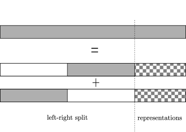
Figure 4: Decomposing a vector using partial representations.

4.3 Presentation of our Algorithm

Plugging representations in Wagner’s algorithm can be done in a variety of ways. The way we achieved our best algorithm was mostly done by trial and error. We present here the main features of our algorithm.

• In the regime we consider, the number of floors $a$ varies from $5$ to $7$. Notice that this is quite larger than in other similar algorithms and is mostly due to the fact that we have many solutions to our Subset Sum problem.

• Because we want to find many solutions, representations become less efficient. Indeed, the fact that we obtain many badly-formed elements makes it harder to find solutions in amortized time $O(1)$ (or even just in small time).

• However, we show that representations can still be useful. For most parameter range, the optimal algorithm consists of a left-right split at the bottom level of the tree, then $2$ layers of partial representation and from there to the top level, left-right splits again.

Figure 5 illustrates an example for $a=7$. When we increase the number of floors, we just add some left-right splits.

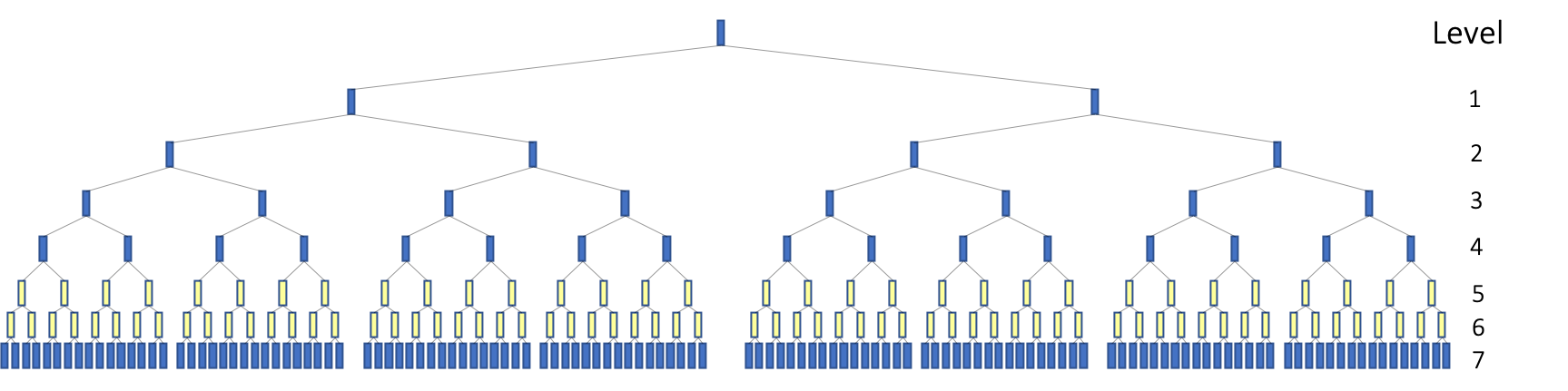
Figure 5: Wagner tree for $a=7$. Yellow list correspond to representations and blue list to left-right splits.

In the next section, we present the different parameters for a particular input to show how our algorithm behaves.

4.4 Application to the Syndrome Decoding Problem

We embedded in the PGE+SS framework the three above-described algorithms, namely the classical Wagner algorithm, the smoothed one in §3 and the one using representation technique in §4. By using Proposition 2, we derived the exponents given in Figures 8 and 9.

We present here the details of our algorithm for the SD$(3,R,W)$ with $R=0.676$ and $W=0.948366$. These are the parameters which are used for the analysis of Wave. For this set of parameters, we claim that the complexity of our algorithm is $2^{0.0176n}$. In the PGE+SS framework (see Section 2.2), we needed to choose to parameters $p$ and $\ell$. We take $\ell=0.060835n$ and $p=k+\ell$.

The best algorithm we found uses $a=7$, which means that the associated Wagner tree has $7$ levels, and therefore $128$ leaves (Figure 5). From level $0$ to level $6$, the lists have size $L=2^{0.0176}$ (i.e. equal to the overall complexity of the Subset Sum problem). As we have more than the required number of solutions for $6$ levels, but not enough for $7$ levels, we use the smoothing method described in section 3.2, which gives a size of the leaves equal to $2^{0.01039}$.

We present below in more detail how we construct the different lists of the Wagner tree.

• Levels 1 to 4 consist of left-right splits. For instance, at level $4$, we have $16$ lists

  $$\forall i\in\llbracket 1,16\rrbracket,\mbox{ }{\mathcal{L}}_{i}\subseteq\left\{\sum_{j\in{\mathcal{I}}_{i}}b_{j}{\mathbf{x}}_{j}\mbox{ }:\mbox{ }\forall j\in{\mathcal{I}}_{i},\;b_{j}\in\{0,1\}\right\}\textrm{ and }|{\mathcal{L}}_{i}|=L.$$

  with ${\mathcal{I}}_{i}\mathop{=}\limits^{\triangle}\ \llbracket 1+\frac{(i-1)({k+\ell})}{16},\frac{i(k+\ell)}{16}\rrbracket$.

• In levels $5$ and $6$, we use partial representations. Going from level $4$ to level $5$, on a proportion $\lambda_{1}=0.7252$ of the vector, we use representations for level $5$ and left-right split for level $6$. On the remaining fraction of the vector, we use representations on both levels. More precisely, for each interval ${\mathcal{I}}_{i}$, we split it in $2$ according to Figure 6. For each part, we use Equation 8 with the following densities:

  • for the part with only one level of representations, $\rho_{1}$ consists on $74.8\%$ of $0$s, $25.1\%$ of $1$s and $0.1\%$ of $2$s;

  • for the part with two levels of representations, we have $\rho_{2}$, composed of $74.2\%$ of $0$s, $25.4\%$ of $1$s and $0.4\%$ of $2$s for level $5$, and $\rho_{3}$ composed of $86.9\%$ of $0$s, $13.1\%$ of $1$s and $0.0\%$ of $2$s for level $6$.

• In order to construct level $7$, we start from each list of level $6$ and perform again a left-right split.

The choice of the densities and all the calculi related to the representations can be quite complicated. We perform a full analysis in Appendix 0.A, see in particular Proposition 5.

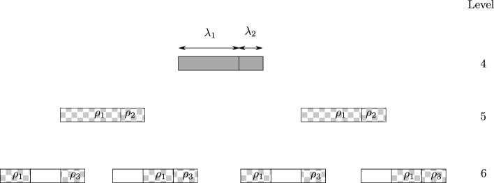
Figure 6: Detail of the floors where we use partial representations.

As explained in section 4.1, most of the elements we build at floors $5$ and $4$ are badly-formed and do not match the desired densities of $0$s, $1$s and $2$s. We only keep the well-formed elements and lower the number of bits on which we merge, so that the merged lists have again $L$ elements. In our case, as the expected number of well-formed elements in level-$4$ lists is $2^{0.0116n}$, we merge on $2^{0.0055n}$ bits to compute the level-$3$ lists (instead of $2^{0.0176n}$ bits.) Similarly, we merge on $2^{0.0173n}$ bits to compute the level-$4$ lists because level-$5$ lists have $2^{0.0174n}$ well-formed elements. This is represented in Figure 7.

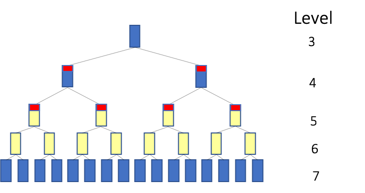
Figure 7: Detail of the bottom floors. Red elements are badly-formed elements.

Finally, level 7 is a left-right split with smaller lists (because of the smoothing). The leaves have size $2^{0.01039n}$, so we merge on $2^{0.0032n}$ bits to build the level-$6$ lists.

The numbers of well-formed elements per list are thus (from level $0$ to level $7$):

$$2^{0.0176n},2^{0.0176n},2^{0.0176n},2^{0.0176n},2^{0.0116n},2^{0.0174n},2^{0.0176n},2^{0.01039n},$$

and the numbers of bits we merge on:

$$2^{0.0176n},2^{0.0176n},2^{0.0176n},2^{0.0055n},2^{0.0173n},2^{0.0176n},2^{0.0032n}.$$

One can check that we merge on a total of $2^{0.0964n}$ bits, which is exactly equal to $2^{\ell\log_{2}(3)}$, meaning that the level-$0$ list is entirely composed of solutions of the Subset Sum problem.

One can also check that the Subset Sum problem has $2^{\ell+k-\ell\log_{2}(3)}=2^{0.6404n}$ solutions, that one solution has $2^{0.4915n}$ representations (see appendix 0.A), and that the merging constraints waste $2^{1.1143n}$ solution representations. We are thus left with $2^{0.0176n}$ solutions, which are exactly the solutions we get on the level-$0$ list.

4.5 Summary of our Results

We present here $2$ plots that illustrate the performance of our different algorithms. What we show is that, in this parameter range, the gain obtained by using representations is relatively small. This is quite surprising because, in the binary case, representations are very efficient. One explanation we have is that, in a regime where there are naturally many solutions, Wagner’s algorithm is very efficient while the representation technique has difficulties in finding solutions in amortized time $O(1)$. In Section 6, we study the hardest instances, and show that representations turn out to be more efficient.

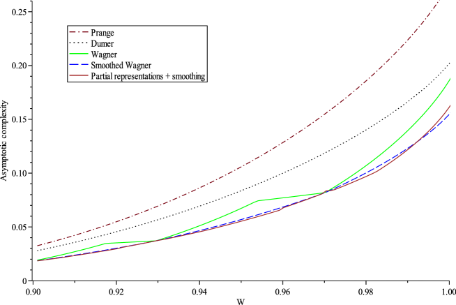
Figure 8: Comparison of the exponent complexities for $R=0.5$

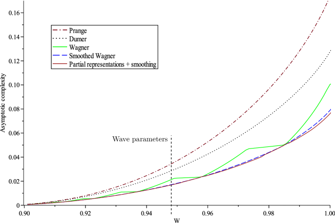
Figure 9: Comparison of the exponent complexities for $R=0.676$

5 New Parameters for the WAVE Signature Scheme

Wave is a new code-based signature scheme proposed in [DST18]. It uses a hash-and-sign approach and follows the GPV paradigm [GPV08] with the instantiation of a code-based preimage sampleable family of functions.

Forging a signature in the Wave scheme amounts to solving the SD problem. Roughly speaking, the public key is a specific pseudo-random parity-check matrix ${\mathbf{H}}$ of size $(n-k)\times n$ and the signature of a message ${\mathbf{m}}$ is an error ${\mathbf{e}}$ of weight $w$ such that ${\mathbf{e}}{{\mathbf{H}}}^{{\mathchoice{\raisebox{0.0pt}{$\displaystyle\intercal$}}{\raisebox{0.0pt}{$\textstyle\intercal$}}{\raisebox{0.0pt}{$\scriptstyle\intercal$}}{\raisebox{0.0pt}{$\scriptscriptstyle\intercal$}}}}=h({\mathbf{m}})$ with $h$ a hash function. However, instead of trying to forge a signature for one message of our choice, a natural idea is to try to forge one message among a selected set of messages. This context leads directly to a slight variation of the classical SD problem. Instead of having one syndrome, there is a list of possible syndromes and the goal is to decode one of them. This problem is known as the Decoding One Out of Many (DOOM) problem.

Problem 4 ()

[Decoding One Out of Many - $\mathrm{DOOM}(n,z,q,R,W)$]

Instance:	${\mathbf{H}}\in\mathbb{F}_{q}^{(n-k)\times n}$ of full rank,
	${\mathbf{s}}_{1},\cdots,{\mathbf{s}}_{z}\in\mathbb{F}_{q}^{n-k}$.
Output:	${\mathbf{e}}\in\mathbb{F}_{q}^{n}\textrm{ and }i\in\llbracket 1,z\rrbracket$ such that $|{\mathbf{e}}|=w$ and ${\mathbf{e}}{{\mathbf{H}}}^{{\mathchoice{\raisebox{0.0pt}{$\displaystyle\intercal$}}{\raisebox{0.0pt}{$\textstyle\intercal$}}{\raisebox{0.0pt}{$\scriptstyle\intercal$}}{\raisebox{0.0pt}{$\scriptscriptstyle\intercal$}}}}={\mathbf{s}}_{i}$,

  

where $k\mathop{=}\limits^{\triangle}\lceil Rn\rceil$, $w\mathop{=}\limits^{\triangle}\lceil Wn\rceil$ and $|{\mathbf{e}}|\mathop{=}\limits^{\triangle}|\{i:{\mathbf{e}}_{i}\neq 0\}|$.

This problem was first considered in [JJ02] and later analyzed for the binary case $(q=2)$ in [Sen11, DST17]. These papers show that one can solve the DOOM problem with an exponential speed-up compared to the $\mathrm{SD}$ problem with equivalent parameters.

The difference induced by DOOM on the PGE+SS framework is that it increases the search space. Namely, instead of searching a solution ${\mathbf{e}}$ of weight $w$ in the space $\left\{{\mathbf{e}}\;:\;{\mathbf{e}}{{\mathbf{H}}}^{{\mathchoice{\raisebox{0.0pt}{$\displaystyle\intercal$}}{\raisebox{0.0pt}{$\textstyle\intercal$}}{\raisebox{0.0pt}{$\scriptstyle\intercal$}}{\raisebox{0.0pt}{$\scriptscriptstyle\intercal$}}}}={\mathbf{s}}\right\}$ we search in $\cup_{i=1}^{z}\left\{{\mathbf{e}}\;:\;{\mathbf{e}}{{\mathbf{H}}}^{{\mathchoice{\raisebox{0.0pt}{$\displaystyle\intercal$}}{\raisebox{0.0pt}{$\textstyle\intercal$}}{\raisebox{0.0pt}{$\scriptstyle\intercal$}}{\raisebox{0.0pt}{$\scriptscriptstyle\intercal$}}}}={\mathbf{s}}_{i}\right\}$.

The idea to solve this problem with Wagner’s approach is to take $z\geq 3^{\ell/a}$ and replace the bottom-right list of the tree ${\mathcal{L}}_{2^{a}}$ by a list containing all the syndromes. Hence, there are only $2^{a}-1$ lists to generate from the search space. Therefore, the constraint of Theorem 3.1 becomes

$$3^{\ell/a}\leq 2^{(k+\ell)/(2^{a}-1)}.$$

For the practical parameters, we have $a=6$ or $a=7$ so the change from $2^{a}$ to $2^{a}-1$ has a negligible impact when we adapt the representation technique to the DOOM problem.

The DOOM parameters stated in [DST18] are derived from the complexity of a key attack detailed in the Wave paper. Our result stated in Section 4.4 provides another attack to consider. We computed the minimal parameters for the Wave scheme so that both attacks would have a time complexity of at least $2^{128}$. They are stated in Table 3 where $n$ is the length of code used in Wave, $k$ its dimension and $w$ the weight of the signature. These should be considered as the new parameters to use for the Wave scheme.

$(n,k,w)$	Public key size (in MB)	Signature length (in kB)
(7236,4892,6862)	2.27	1.434

Table 3: New parameters of the Wave signature scheme for $128$ bits of security.

6 Hardest Instances of Ternary Syndrome Decoding

In the previous sections, we tried to optimize our algorithms for the regime of parameters used in the Wave signature scheme. The corresponding Syndrome Decoding problem uses $R=0.676$ and $w\approx 0.948$. This corresponds to a regime where there are many solutions to the problem and hence Wagner’s algorithm with a large number of floors was efficient. However, this is not the problem where the problem is the hardest.

We will now look at the hardest instances of the ternary Syndrome Decoding in large weight. As we already teased in the introduction, ternary SD is much harder in large weights than in small weights. In the two examples we considered, namely $R=0.5$ and $R=0.676$, the problem was the hardest for $W=1$. As we will see, there are some lower rates for which the complexity of the Syndrome Decoding problem is maximal for $W<1$.

Consider an instance $({\mathbf{H}},{\mathbf{s}})$ of SD$(3,R,W)$ with $W\geq\frac{2}{3}$. We have ${\mathbf{H}}\in\mathbb{F}_{3}^{(n-k)\times n}$ of full rank and ${\mathbf{s}}\in\mathbb{F}_{3}^{n-k}$. As in the binary case, the problem is the hardest when it has a unique solution on average, if such a regime exists.

Let $R_{\textup{max}}\mathop{=}\limits^{\triangle}\frac{\log_{2}(3)-1}{\log_{2}(3)}\approx 0.36907$. For $R\in[0,R_{\textup{max}}]$, we define $W_{\textup{GV}}^{\textup{high}}(R)$ as the only value in $[2/3,1]$ such that

$$W_{\textup{GV}}^{\textup{high}}(R)+h_{2}(W_{\textup{GV}}^{\textup{high}}(R))=(1-R)\log_{2}(3),$$

where $h_{2}(x)\mathop{=}\limits^{\triangle}-x\log_{2}(x)-(1-x)\log_{2}(1-x)$.

The rate $R_{\textup{max}}$ was defined such that $W_{\textup{GV}}^{high}(R_{\textup{max}})=1$, while this quantity is not defined for $R>R_{\textup{max}}$. This is why Figures 8 and 9 do not show a high peak for $R=0.5$ and $R=0.676$ but an increasing function up to $W=1$. By Proposition 1, quantity $W_{\textup{GV}}^{\textup{high}}(R)$ corresponds to the relative weight for which we expect one solution to $SD$ with rate $R$ and $q=3$.

In order to study the above problem for hard high weight instances, we compared the performance of $3$ standard algorithms: Prange’s algorithm, Dumer’s algorithm and the BJMM algorithm.

We performed a case study and showed that, for all the above-mentioned algorithms, the hardest case is reached for $R=R_{\textup{max}}\approx 0.36907$ and $W=1$. We obtain the following results.

Algorithm	$q=2$	$q=3$ and $W>0.5$
Prange	0.121 ($R$ = 0.454)	0.369 ($R$ = 0.369)
Dumer/Wagner	0.116 ($R$ = 0.447)	0.269 ($R$ = 0.369)
BJMM/our algorithm	0.102 ($R$ = 0.427)	0.247 ($R$ = 0.369)

Table 4: Best exponents with associated rates.

In both the binary and the ternary case, we can see that Prange’s algorithm performs very poorly, but that Dumer’s algorithm already gives much better results and that BJMM’s Subset Sum techniques, using representations, increases the gain. The analysis of Prange and Dumer for $q=3$ is quite straightforward and follows closely the binary case. For BJMM (i.e. Wagner’s algorithm with representations), the exponent $0.247$ comes from a $2$-levels Wagner tree that includes $1$ layer of representations. We tried using a larger Wagner trees but this did not give any improvement.

The ternary SD appears significantly harder than its binary counterpart. This was expected to some extent because in the ternary case, the input matrices have elements in $\mathbb{F}_{3}$ and not $\mathbb{F}_{2}$, which means that matrices of the same dimension contain more information.

In order to confirm this idea, we define the following metric: what is the smallest input size for which the algorithms need at least $2^{128}$ operations to decode? We use the value $128$, as $128$ security bits is a cryptographic standard. The input matrix ${\mathbf{H}}\in\mathbb{F}_{3}^{n(1-R)\times n}$ is represented in systematic form. This means that we write

$${\mathbf{H}}=\begin{pmatrix}{\boldsymbol{1}}_{n(1-R)}&{\mathbf{H}}^{\prime}\end{pmatrix}.$$

The only relevant part that needs to be specified is ${\mathbf{H}}^{\prime}$. This requires $R(1-R)n^{2}\log_{2}(q)$ bits. We show that, even in this metric, the ternary syndrome decoding problem is much harder, i.e. requires $2^{128}$ operations to decode inputs of much smaller sizes. Our results are summarized in the table below.

Algorithm	$q=2$	$q=3$ and $W>0.5$
Prange	275 ($R$ = 0.384)	44 ($R$ = 0.369)
Dumer/Wagner	295 ($R$ = 0.369)	83 ($R$ = 0.369)
BJMM/our algorithm	374 ($R$ = 0.326)	99 ($R$ = 0.369)

Table 5: Minimum input sizes (in Kbits) for a time complexity of $2^{128}$.

Notice that in this metric, in the binary case, it is worth reducing the rate $R$, as this reduces the input size. But in the ternary case, we do not observe this behavior, which shows that the problem quickly becomes simple, as $R$ decreases.

The work we present here is very preliminary but opens many new perspectives. It seems there are many cases in code-based cryptography, from encryption schemes to signatures, where this problem could replace the binary Syndrome Decoding problem to get smaller key sizes.

7 Conclusion

In this work, we stressed a strong difference between the cases $q=2$ and $q\geq 3$ of the Syndrome Decoding problem. Namely, the symmetry between the small weight and the large weight cases, which occurs in the binary case, is broken for larger values of $q$. The large weight case of the general Syndrome Decoding problem had never been studied before. We proposed two algorithms to solve the Syndrome Decoding problem in this new regime in the context of the Partial Gaussian Elimination and Subset Sum framework. Our first algorithm uses a $q$-ary version of Wagner’s approach to solve the underlying Subset Sum problem. We proposed a second algorithm making use of representations as in the BJMM approach. We studied both algorithms and proposed a first application for cryptographic purposes, namely for the Wave signature scheme. Considering our complexity analysis, we proposed new parameters for this scheme. Furthermore, we showed that the worst case complexity of Syndrome Decoding in large weight is higher than in small weight. This implies that it should be possible to develop new code-based cryptographic schemes using this regime of parameters that reach the same security level with smaller key size.

Appendix 0.A Appendix: Ternary Representations

In this section, we explain how to compute the number of representations as well as the number of badly-formed vectors when using ternary representations.

0.A.1 Notations

The notation $\begin{pmatrix}n\\ k_{1},\dots,k_{i}\end{pmatrix}$ will denote the multinomial coefficient $\dfrac{n!}{k_{1}!\dots k_{i}!}$, assuming that $n=k_{1}+\dots+k_{i}$.

Let us denote $g:(n,k_{1},k_{2})\rightarrow n\log_{2}(n)-k_{1}\log_{2}(k_{1})-k_{2}\log_{2}(k_{2})-(n-k_{1}-k_{2})\log_{2}(n-k_{1}-k_{2})$. We have:

$$\begin{pmatrix}n\\ k_{1},k_{2},n-k_{1}-k_{2}\end{pmatrix}=\tilde{O}\left(2^{g(n,k_{1},k_{2})}\right).$$

The function $g$ satisfies :

• $g(n,k_{1},k_{2})=g(n,k_{2},k_{1})$,

• $g(n,k_{1},k_{2})=g(n,k_{1},n-k_{1}-k_{2})$,

• $g(\lambda n,\lambda k_{1},\lambda k_{2})=\lambda g(n,k_{1},k_{2})$,

• $g(n,k_{1},k_{2})=nh_{2}\left(\frac{k_{1}+k_{2}}{n}\right)+(k_{1}+k_{2})h_{2}\left(\frac{k_{1}}{k_{1}+k_{2}}\right)$, where $h_{2}$ stands for the binary entropy.

We denote by $T(n,\alpha,\beta)$ the set of all vectors of length $n$ composed with $\alpha n$ $1$s, $\beta n$ $2$s and $(1-\alpha-\beta)n$ $0$s. There exist $\begin{pmatrix}n\\ \alpha n$, $\beta n$, $(1-\alpha-\beta)n\end{pmatrix}=\tilde{O}\left(2^{ng(1,\alpha,\beta)}\right)$ such vectors.

0.A.2 Main Result

The goal of this section is to prove the following result.

Proposition 5

For $\mathbf{b}\in T(n,\alpha_{0},\beta_{0})$, the number of way one can decompose $\mathbf{b}$ as the sum of two vectors from $T(n,\alpha_{1},\beta_{1})$ is given by:

$$\tilde{O}\left(2^{n(g(1-\alpha_{0}-\beta_{0},\overline{x}_{12},\overline{x}_{12})+g(\alpha_{0},\overline{x}_{01},\overline{x}_{01})+g(\beta_{0},\overline{x}_{02},\overline{x}_{02}))}\right),$$

where

$$\begin{array}[]{cl}\overline{x}_{01}=&\dfrac{2\alpha_{0}+\beta_{0}-\alpha_{1}-2\beta_{1}}{3}+z\\ \overline{x}_{02}=&\dfrac{\alpha_{0}+2\beta_{0}-2\alpha_{1}-\beta_{1}}{3}+z\\ \overline{x}_{12}=&z\\ \end{array}$$

and $z$ is the real root of

$$\dfrac{(2\alpha_{0}+\beta_{0}-\alpha_{1}-2\beta_{1}+3z)(\alpha_{0}+2\beta_{0}-2\alpha_{1}-\beta_{1}+3z)z}{(1-\alpha_{0}-\beta_{0}-2z)(-2\alpha_{0}-\beta_{0}+4\alpha_{1}+2\beta_{1}-6z)(-\alpha_{0}-2\beta_{0}+2\alpha_{1}+4\beta_{1}-6z)}=1.$$

0.A.3 A Simple Example

Let us consider a very simple case: we want to decompose a balanced vector of size $n$ (the number of $0$s, $1$s and $2$s is $n/3$) in two balanced vectors (i.e. $\alpha_{0}=\beta_{1}=\alpha_{1}=\beta_{1}=1/3$). There are several ways to achieve this. One solution is that each $0$ is obtain by $0+0$, each $1$ by $2+2$, and each $2$ by $1+1$. There is exactly only one way to build the vector in this way. Another possibility is that each case ($0+0$, $1+2$, $2+1$, $1+0$, $2+2$, $0+1$, $2+0$, $0+2$ and $1+1$) happens $n/9$ times. This is the scenario admitting the maximal number of decompositions: $\tilde{O}\left(3^{n}\right)$. There are many more possibilities.

The number of representations is the sum of all decompositions for all the possible scenarios. There are only a polynomial number of different scenarios. The total number of representations (which is what we want to determine) is determined, up to a polynomial factor, by the scenario which gives the maximal number of decompositions. In this case, there are $\tilde{O}\left(3^{n}\right)$ representations.

Let us check that this is the result givent by Proposition 5. Indeed, in this case, $z$ must satisfy the equation

$$\frac{(3z)(3z)z}{(1/3-2z)(1-6z)(1-6z)}=1,\text{ or equivalently }27z^{3}=(1-6z)^{3}.$$

The real root of this equation is $1/9$. Thus we obtain $\overline{x}_{01}=\overline{x}_{02}=\overline{x}_{12}=1/9$. Finally, the number of representations is

$$\tilde{O}\left(2^{3ng(1/3,1/9,1/9)}\right)=\tilde{O}\left(2^{3n\times(\log_{2}(3)/3)}\right)=\tilde{O}\left(3^{n}\right).$$

0.A.4 Typical Case

In general, we have a vector ${\mathbf{b}}\in T(n,\alpha_{0},\beta_{0})$. We want to decompose it into two vectors of $T(n,\alpha_{1},\beta_{1})$. Let us call $x_{00},\dots,x_{22}$ the density of the nine cases ($0+0$, $0+1$, $\dots$, $2+2$) as shown in the following table :

$$\begin{array}[]{p{3mm}|ccc}&0&1&2\\ \hline\cr 0&x_{00}&x_{01}&x_{02}\\ 1&x_{10}&x_{11}&x_{12}\\ 2&x_{20}&x_{21}&x_{22}\end{array}$$

We denote by $\mathcal{A}$ the set of possible such tuples $x_{00},\dots,x_{22}$.

Given the target vector $\mathbf{b}$, there are $\begin{pmatrix}n(1-\alpha_{0}-\beta_{0})\\ nx_{00},nx_{12},nx_{21}\end{pmatrix}\begin{pmatrix}n\alpha_{0}\\ nx_{01},nx_{10},nx_{22}\end{pmatrix}\begin{pmatrix}n\beta_{0}\\ nx_{02},nx_{11},nx_{20}\end{pmatrix}$ ways of decomposing this $\mathbf{b}$ according to $(x_{00},\dots,x_{22})$. Indeed, a $0$ in $\mathbf{b}$ can be decomposed as $0+0$ (this happens $nx_{00}$ times), $1+2$ ($nx_{12}$ times) or $2+1$ ($nx_{21}$ times). As the number of $0s$ in $\mathbf{b}$ is $n(1-\alpha_{0}-\beta_{0})$, there are $\begin{pmatrix}n(1-\alpha_{0}-\beta_{0})\\ nx_{00},nx_{12},nx_{21}\end{pmatrix}$ ways to choose the decomposition of each $0$ of $\mathbf{b}$. The choices of the decompositions of the $1$s and the $2$s give the other two factors.

For given $\alpha_{0},\beta_{0},\alpha_{1}$ and $\beta_{1}$, the number of possible decompositions is

$$\sum\limits_{(x_{00},\dots,x_{22})\in\mathcal{A}}\begin{pmatrix}n(1-\alpha_{0}-\beta_{0})\\ nx_{00},nx_{12},nx_{21}\end{pmatrix}\begin{pmatrix}n\alpha_{0}\\ nx_{01},nx_{10},nx_{22}\end{pmatrix}\begin{pmatrix}n\beta_{0}\\ nx_{02},nx_{11},nx_{20}\end{pmatrix}.$$

Up to a polynomial factorm this is equal to

$$\sum\limits_{(x_{00},\dots,x_{22})\in\mathcal{A}}2^{n(g(1-\alpha_{0}-\beta_{0},x_{21},x_{12})+g(\alpha_{0},x_{01},x_{10})+g(\beta_{0},x_{02},x_{20}))}.$$

The largest term (or eventually one of the largest terms) of this sum is

$$2^{n(g(1-\alpha_{0}-\beta_{0},\overline{x}_{21},\overline{x}_{12})+g(\alpha_{0},\overline{x}_{01},\overline{x}_{10})+g(\beta_{0},\overline{x}_{02},\overline{x}_{20}))},$$

where $(\overline{x}_{00},\dots,\overline{x}_{22})$ is called the typical case.

We are interested in this typical case because it gathers a polynomial fraction of all the possible decompositions. The asymptotic exponent of the total number of representations is then simply given by the exponent of the typical case.

0.A.5 Computation of the Typical Case

Given $\alpha_{0},\beta_{0},\alpha_{1}$ and $\beta_{1}$, the following constraints exist on $x_{00},\dots,x_{22}$.

$$\begin{array}[]{ccl}x_{00}+x_{01}+x_{02}&=&1-\alpha_{1}-\beta_{1}\\ x_{10}+x_{11}+x_{12}&=&\alpha_{1}\\ x_{20}+x_{21}+x_{22}&=&\beta_{1}\\ \\ x_{00}+x_{10}+x_{20}&=&1-\alpha_{1}-\beta_{1}\\ x_{01}+x_{11}+x_{21}&=&\alpha_{1}\\ x_{02}+x_{12}+x_{22}&=&\beta_{1}\\ \\ x_{00}+x_{12}+x_{21}&=&1-\alpha_{0}-\beta_{0}\\ x_{01}+x_{10}+x_{22}&=&\alpha_{0}\\ x_{02}+x_{11}+x_{20}&=&\beta_{0}\\ \end{array}$$

However, these equations are not independent. Each of the three sets of three equations implies $x_{00}+\dots+x_{22}=1$. We are actually left with two degrees of freedom, and any solution can be written as

$$\begin{array}[]{ccccccc}x_{00}&=&1-\alpha_{0}-\beta_{0}&-&2z\\ x_{01}&=&\dfrac{2\alpha_{0}+\beta_{0}-\alpha_{1}-2\beta_{1}}{3}&+&z&+&w\\ x_{02}&=&\dfrac{\alpha_{0}+2\beta_{0}-2\alpha_{1}-\beta_{1}}{3}&+&z&-&w\\ x_{10}&=&\dfrac{2\alpha_{0}+\beta_{0}-\alpha_{1}-2\beta_{1}}{3}&+&z&-&w\\ x_{11}&=&\dfrac{-2\alpha_{0}-\beta_{0}+4\alpha_{1}+2\beta_{1}}{3}&-&2z\\ x_{12}&=&0&+&z&+&w\\ x_{20}&=&\dfrac{\alpha_{0}+2\beta_{0}-2\alpha_{1}-\beta_{1}}{3}&+&z&+&w\\ x_{21}&=&0&+&z&-&w\\ x_{22}&=&\dfrac{-\alpha_{0}-2\beta_{0}+2\alpha_{1}+4\beta_{1}}{3}&-&2z.\end{array}$$

Thus, $\mathcal{A}=\{(x_{00}(w,z),\dots,x_{22}(w,z))\;|\;\forall(i,j),x_{ij}\geqslant 0\}$.

Determining $w$.

In a first step, we will show that the typical case must be symmetric (i.e. $\overline{x}_{01}=\overline{x}_{10}$, $\overline{x}_{02}=\overline{x}_{20}$ and $\overline{x}_{12}=\overline{x}_{21}$), which means that $w$ must be $0$. To do so, we consider a pair $(w,z)$ such that the corresponding $(x_{00},\dots,x_{22})$ is in $\mathcal{A}$, and we call $(\tilde{x}_{00},\dots,\tilde{x}_{22})$ the solution with the same $z$ but $0$ instead of $w$.

As $(x_{00},\dots,x_{22})$ is in $\mathcal{A}$, all $x_{ij}$ are positive or zero. This implies that all $\tilde{x}_{ij}$ are positive or zero. For example, for $\tilde{x}_{01}$ we have:

$$0\leqslant\min(x_{01},x_{10})=\tilde{x}_{01}-\operatorname{abs}(w)\leqslant\tilde{x}_{01}.$$

Therefore, $(\tilde{x}_{00},\dots,\tilde{x}_{22})$ is in $\mathcal{A}$ and we obtain

$$\dfrac{\operatorname{Nrep}(\mathbf{\tilde{x}})}{\operatorname{Nrep}(\mathbf{x})}=\dfrac{2^{n(g(1-\alpha_{0}-\beta_{0},\tilde{x}_{21},\tilde{x}_{12})+g(\alpha_{0},\tilde{x}_{01},\tilde{x}_{10})+g(\beta_{0},\tilde{x}_{02},\tilde{x}_{20}))}}{2^{n(g(1-\alpha_{0}-\beta_{0},x_{21},x_{12})+g(\alpha_{0},x_{01},x_{10})+g(\beta_{0},x_{02},x_{20}))}}.$$ (9)

But we have the following equality.

$$\begin{array}[]{ccl}g(1-\alpha_{0}-\beta_{0},x_{21},x_{12})&=&g(1-\alpha_{0}-\beta_{0},\tilde{x}_{12}+w,\tilde{x}_{12}-w)\\ &=&g(1-\alpha_{0}-\beta_{0},\tilde{x}_{12},\tilde{x}_{12})+2\tilde{x}_{21}\left(h(1/2+w/\tilde{x}_{12})-h(1/2)\right).\end{array}$$

Similarly, we obtain two other formulas.

$$g(\alpha_{0},x_{01},x_{10})=g(\alpha_{0},\tilde{x}_{01},\tilde{x}_{10})+2\tilde{x}_{01}\left(h(1/2+w/\tilde{x}_{01})-h(1/2)\right),$$

$$g(\beta_{0},x_{02},x_{20})=g(\beta_{0},\tilde{x}_{02},\tilde{x}_{20})+2\tilde{x}_{02}\left(h(1/2+w/\tilde{x}_{02})-h(1/2)\right).$$

Therefore, we can reduce Equation 9 to

$$\dfrac{\operatorname{Nrep}(\mathbf{\tilde{x}})}{\operatorname{Nrep}(\mathbf{x})}=2^{2n\left(\tilde{x}_{01}\left(1-h\left(\frac{1}{2}+\frac{w}{\tilde{x}_{01}}\right)\right)+\tilde{x}_{02}\left(1-h\left(\frac{1}{2}+\frac{w}{\tilde{x}_{02}}\right)\right)+\tilde{x}_{12}\left(1-h\left(\frac{1}{2}+\frac{w}{\tilde{x}_{12}}\right)\right)\right)}.$$

So $\operatorname{Nrep}(\mathbf{x})\leqslant\operatorname{Nrep}(\mathbf{\tilde{x}})$ and these two quantities are equal if and only $w=0$, i.e. $\mathbf{x}=\mathbf{\tilde{x}}$.

Determining $z$.

To get the typical case, we now have to find the value of $z$ that maximises the expression

$$g(1-\alpha_{0}-\beta_{0},x_{21},x_{12})+g(\alpha_{0},x_{01},x_{10})+g(\beta_{0},x_{02},x_{20}).$$

Notice that this expression is equivalent, up to an additive constant, to $-\sum\limits_{i,j}x_{ij}\log_{2}(x_{ij})$.

This function is concave and thus admit a single maximum. The differentiation of this function with respect to $z$ gives

$$-2\log_{2}\left(\dfrac{\left(\dfrac{2\alpha_{0}+\beta_{0}-\alpha_{1}-2\beta_{1}}{3}+z\right)\left(\dfrac{\alpha_{0}+2\beta_{0}-2\alpha_{1}-\beta_{1}}{3}+z\right)z}{\left(1-\alpha_{0}-\beta_{0}-2z\right)\left(\dfrac{-2\alpha_{0}-\beta_{0}+4\alpha_{1}+2\beta_{1}}{3}-2z\right)\left(\dfrac{-\alpha_{0}-2\beta_{0}+2\alpha_{1}+4\beta_{1}}{3}-2z\right)}\right),$$

which is equal to zero if and only if

$$\dfrac{(2\alpha_{0}+\beta_{0}-\alpha_{1}-2\beta_{1}+3z)(\alpha_{0}+2\beta_{0}-2\alpha_{1}-\beta_{1}+3z)z}{(1-\alpha_{0}-\beta_{0}-2z)(-2\alpha_{0}-\beta_{0}+4\alpha_{1}+2\beta_{1}-6z)(-\alpha_{0}-2\beta_{0}+2\alpha_{1}+4\beta_{1}-6z)}=1.$$

This explains why $z$ is the root of a polynomial of degree $3$.

0.A.6 Number of Representations and Badly-formed Elements

There are $\tilde{O}\left(2^{ng(1,\alpha_{0},\beta_{0})}\right)$ vectors in $T(n,\alpha_{0},\beta_{0})$. For each of these vectors, there are by definition $\operatorname{Nrep}(\alpha_{0},\beta_{0},\alpha_{1},\beta_{1})$ ways of decomposing it as the sum of two vectors of $T(n,\alpha_{1},\beta_{1})$. Moreover, the number of vectors in $T(n,\alpha_{1},\beta_{1})$ is $\tilde{O}\left(2^{ng(1,\alpha_{1},\beta_{1})}\right)$. There are then $\tilde{O}\left(2^{2ng(1,\alpha_{1},\beta_{1})}\right)$ pairs of vectors of $T(n,\alpha_{1},\beta_{1})$, but only $\tilde{O}\left(\operatorname{Nrep}(\alpha_{0},\beta_{0},\alpha_{1},\beta_{1})2^{ng(1,\alpha_{0},\beta_{0})}\right)$ of these pairs give a valid representation of a vector of $T(n,\alpha_{0},\beta_{0})$. All the other pairs give badly-formed elements. Thus, when we merge two $L$-sized lists of elements of $T(n,\alpha_{1},\beta_{1})$ on $L$ bits, we obtain $\tilde{O}\left(L\operatorname{Nrep}(\alpha_{0},\beta_{0},\alpha_{1},\beta_{1})2^{ng(1,\alpha_{0},\beta_{0})-2ng(1,\alpha_{1},\beta_{1})}\right)$ vectors of $T(n,\alpha_{0},\beta_{0})$, the remaining consisting on badly-formed vectors.

References

• [ABB+17] Nicolas Aragon, Paulo Barreto, Slim Bettaieb, Loic Bidoux, Olivier Blazy, Jean-Christophe Deneuville, Phillipe Gaborit, Shay Gueron, Tim Güneysu, Carlos Aguilar Melchor, Rafael Misoczki, Edoardo Persichetti, Nicolas Sendrier, Jean-Pierre Tillich, and Gilles Zémor. BIKE, December 2017. NIST Round 1 submission for Post-Quantum Cryptography.
• [ACP+17] Martin Albrecht, Carlos Cid, Kenneth G. Paterson, Cen Jung Tjhai, and Martin Tomlinson. NTS-KEM. first round submission to the NIST post-quantum cryptography call, December 2017.
• [AMAB+17] Carlos Aguilar Melchor, Nicolas Aragon, Slim Bettaieb, Loïc Bidoux, Olivier Blazy, Jean-Christophe Deneuville, Philippe Gaborit, Edoardo Persichetti, and Gilles Zémor. HQC, December 2017. NIST Round 1 submission for Post-Quantum Cryptography.
• [BBC+19] Marco Baldi, Alessandro Barenghi, Franco Chiaraluce, Gerardo Pelosi, and Paolo Santini. LEDAcrypt. second round submission to the NIST post-quantum cryptography call, January 2019.
• [BCJ11] Anja Becker, Jean-Sébastien Coron, and Antoine Joux. Improved generic algorithms for hard knapsacks. In Advances in Cryptology - EUROCRYPT 2011 - 30th Annual International Conference on the Theory and Applications of Cryptographic Techniques, Tallinn, Estonia, May 15-19, 2011. Proceedings, pages 364–385, 2011.
• [BCL+17] Daniel J. Bernstein, Tung Chou, Tanja Lange, Ingo von Maurich, Ruben Niederhagen, Edoardo Persichetti, Christiane Peters, Peter Schwabe, Nicolas Sendrier, Jakub Szefer, and Wang Wen. Classic McEliece: conservative code-based cryptography. https://csrc.nist.gov/CSRC/media/Projects/Post-Quantum-Cryptography/documents/round-1/submissions/Classic_McEliece.zip, November 2017. First round submission to the NIST post-quantum cryptography call.
• [BJMM12] Anja Becker, Antoine Joux, Alexander May, and Alexander Meurer. Decoding random binary linear codes in $2^{n/20}$: How $1+1=0$ improves information set decoding. In Advances in Cryptology - EUROCRYPT 2012, LNCS. Springer, 2012.
• [BMvT78] Elwyn Berlekamp, Robert McEliece, and Henk van Tilborg. On the inherent intractability of certain coding problems. IEEE Trans. Inform. Theory, 24(3):384–386, May 1978.
• [CFG89] Mark Chaimovich, Gregory Freiman, and Zvi Galil. Solving dense subset-sum problems by using analytical number theory. J. Complexity, 5(3):271–282, 1989.
• [CFS01] Nicolas Courtois, Matthieu Finiasz, and Nicolas Sendrier. How to achieve a McEliece-based digital signature scheme. In Advances in Cryptology - ASIACRYPT 2001, volume 2248 of LNCS, pages 157–174, Gold Coast, Australia, 2001. Springer.
• [CG90] John T Coffey and Rodney M Goodman. The complexity of information set decoding. IEEE Transactions on Information Theory, 36(5):1031–1037, 1990.
• [CT17] Rodolfo Canto Torres. Asymptotic analysis of ISD algorithms for the $q-$ary case. In Proceedings of the Tenth International Workshop on Coding and Cryptography WCC 2017, September 2017.
• [DST17] Thomas Debris-Alazard, Nicolas Sendrier, and Jean-Pierre Tillich. Surf: a new code-based signature scheme. preprint, September 2017. arXiv:1706.08065v3.
• [DST18] Thomas Debris-Alazard, Nicolas Sendrier, and Jean-Pierre Tillich. Wave: A new code-based signature scheme. Cryptology ePrint Archive, Report 2018/996, October 2018. https://eprint.iacr.org/2018/996.
• [Dum91] Ilya Dumer. On minimum distance decoding of linear codes. In Proc. 5th Joint Soviet-Swedish Int. Workshop Inform. Theory, pages 50–52, Moscow, 1991.
• [FP05] Abraham Flaxman and Bartosz Przydatek. Solving medium-density subset sum problems in expected polynomial time. In STACS 2005, 22nd Annual Symposium on Theoretical Aspects of Computer Science, Stuttgart, Germany, February 24-26, 2005, Proceedings, pages 305–314, 2005.
• [GKH17] Cheikh Thiécoumba Gueye, Jean Belo Klamti, and Shoichi Hirose. Generalization of BJMM-ISD using may-ozerov nearest neighbor algorithm over an arbitrary finite field \mathbb f_q. In Codes, Cryptology and Information Security - Second International Conference, C2SI 2017, Rabat, Morocco, April 10-12, 2017, Proceedings - In Honor of Claude Carlet, pages 96–109, 2017.
• [GM91] Zvi Galil and Oded Margalit. An almost linear-time algorithm for the dense subset-sum problem. SIAM J. Comput., 20(6):1157–1189, 1991.
• [GPV08] Craig Gentry, Chris Peikert, and Vinod Vaikuntanathan. Trapdoors for hard lattices and new cryptographic constructions. In Proceedings of the fortieth annual ACM symposium on Theory of computing, pages 197–206. ACM, 2008.
• [Hir16] Shoichi Hirose. May-ozerov algorithm for nearest-neighbor problem over $\mathbb{f}$ ${}_{\mbox{q}}$ and its application to information set decoding. In Innovative Security Solutions for Information Technology and Communications - 9th International Conference, SECITC 2016, Bucharest, Romania, June 9-10, 2016, Revised Selected Papers, pages 115–126, 2016.
• [HJ10] Nicholas Howgrave-Graham and Antoine Joux. New generic algorithms for hard knapsacks. In Henri Gilbert, editor, Advances in Cryptology - EUROCRYPT 2010, volume 6110 of LNCS. Sringer, 2010.
• [IKR+18] Carmelo Interlando, Karan Khathuria, Nicole Rohrer, Joachim Rosenthal, and Violetta Weger. Generalization of the ball-collision algorithm. arXiv preprint arXiv:1812.10955, 2018.
• [JJ02] Thomas Johansson and Fredrik Jönsson. On the complexity of some cryptographic problems based on the general decoding problem. IEEE Trans. Inform. Theory, 48(10):2669–2678, October 2002.
• [Lyu05] Vadim Lyubashevsky. On random high density subset sums. Electronic Colloquium on Computational Complexity (ECCC), 1(007), 2005.
• [McE78] Robert J. McEliece. A Public-Key System Based on Algebraic Coding Theory, pages 114–116. Jet Propulsion Lab, 1978. DSN Progress Report 44.
• [Meu17] Alexander Meurer. A Coding-Theoretic Approach to Cryptanalysis. PhD thesis, Ruhr University Bochum, November 2017.
• [MMT11] Alexander May, Alexander Meurer, and Enrico Thomae. Decoding random linear codes in $O(2^{0.054n})$. In Dong Hoon Lee and Xiaoyun Wang, editors, Advances in Cryptology - ASIACRYPT 2011, volume 7073 of LNCS, pages 107–124. Springer, 2011.
• [MTSB12] Rafael Misoczki, Jean-Pierre Tillich, Nicolas Sendrier, and Paulo S. L. M. Barreto. MDPC-McEliece: New McEliece variants from moderate density parity-check codes. IACR Cryptology ePrint Archive, Report2012/409, 2012, 2012.
• [Pet10] Christiane Peters. Information-set decoding for linear codes over ${\mathbf{F}}_{q}$. In Post-Quantum Cryptography 2010, volume 6061 of LNCS, pages 81–94. Springer, 2010.
• [Pra62] Eugene Prange. The use of information sets in decoding cyclic codes. IRE Transactions on Information Theory, 8(5):5–9, 1962.
• [Sen11] Nicolas Sendrier. Decoding one out of many. In Post-Quantum Cryptography 2011, volume 7071 of LNCS, pages 51–67, 2011.
• [Ste93] Jacques Stern. A new identification scheme based on syndrome decoding. In D.R. Stinson, editor, Advances in Cryptology - CRYPTO’93, volume 773 of LNCS, pages 13–21. Springer, 1993.
• [Wag02] David Wagner. A generalized birthday problem. In Moti Yung, editor, Advances in Cryptology - CRYPTO 2002, volume 2442 of LNCS, pages 288–303. Springer, 2002.