Scene Segmentation-Based Luminance Adjustment
for Multi-Exposure Image Fusion
Abstract
We propose a novel method for adjusting luminance for multi-exposure image fusion. For the adjustment, two novel scene segmentation approaches based on luminance distribution are also proposed. Multi-exposure image fusion is a method for producing images that are expected to be more informative and perceptually appealing than any of the input ones, by directly fusing photos taken with different exposures. However, existing fusion methods often produce unclear fused images when input images do not have a sufficient number of different exposure levels. In this paper, we point out that adjusting the luminance of input images makes it possible to improve the quality of the final fused images. This insight is the basis of the proposed method. The proposed method enables us to produce high-quality images, even when undesirable inputs are given. Visual comparison results show that the proposed method can produce images that clearly represent a whole scene. In addition, multi-exposure image fusion with the proposed method outperforms state-of-the-art fusion methods in terms of MEF-SSIM, discrete entropy, tone mapped image quality index, and statistical naturalness.
Index Terms:
Multi-exposure image fusion, luminance adjustment, image enhancement, image segmentationI Introduction
The low dynamic range (LDR) of the imaging sensors used in modern digital cameras is a major factor preventing cameras from capturing images as good as human vision. This is due to the limited dynamic range that imaging sensors have, and a single shutter speed that is utilized when we take photos. The limitations result in low-contrast images taken by digital cameras. To obtain images with better quality, numerous imaging and enhancement techniques based on a single image have been proposed [1, 2, 3, 4, 5, 6]. However, these techniques cannot restore saturated pixel values in LDR images.
Because of this situation, interest in multi-image-based imaging techniques [7, 8, 9, 10, 11, 12, 13, 14, 15, 16, 17] has been increasing to overcome this constraint that single-image-based techniques have. Multi-exposure image fusion is a solution to the LDR problem of digital cameras. Fusion methods utilize a set of differently exposed images, called “multi-exposure images,” and fuse them to produce an image with high quality. Their development was inspired by high dynamic range (HDR) imaging techniques [18, 19, 20, 21, 22, 23, 24, 25, 26, 27]. The advantage of these methods, compared with HDR imaging techniques, is that they can eliminate three operations: generating HDR images, calibrating the camera response function (CRF), and preserving the exposure value of each photograph. In this paper, we focus on multi-exposure image fusion.
However, to work well, existing fusion methods require two conditions [28, 29]: input multi-exposure images include no moving artifacts such as blurring or misalignment among images, and input multi-exposure images clearly cover the dynamic range of a scene. Moreover, the conditions have a close relation each other. To capture multi-exposure images covering a high dynamic range, it is generally needed to shoot multiple times while changing the shutter speed. In this case, moving artifacts generally occur due to time lags of each shooting and long-shutter speeds to capture bright images. Therefore, the two conditions are not always satisfied at the same time in various practical situations.
For eliminating moving artifacts among images, specialized camera systems [30, 31] and a number of robust fusion methods [32] have been studied. For specialized camera systems, spatially varying pixel exposure methods [30, 31] using a single sensor and new optical systems [33, 34] having a number of sensors have been proposed. These systems enable us to capture scenes at the same time by changing the amount of light absorbed at each pixel in the imaging sensor, or by varying the exposure for each sensor. However, these camera systems do not always capture images having a sufficient number of different exposure levels, due to the hardware limitation of camera systems.
In contrast, for robust fusion methods against moving artifacts, input multi-exposure images taken with conventional cameras are first aligned, and then aligned images are fused. These methods effectively produce high-quality images even when scenes include moving objects, if well-exposed multi-exposure images are prepared. However, the quality of input multi-exposure images affects both the accuracy of image alignment and the performance of fusion. Hence, insufficient multi-exposure images, such as ones taken with fast-shutter-speed due to limitations of camera capability, make it difficult to produce high-quality results. Because of these situations, we aim to propose a scene segmentation-based luminance adjustment method, for improving the quality of insufficient multi-exposure images.
In this paper, we first point out that it is possible to improve the quality of multi-exposure images by adjusting the luminance of images after photographing. Moreover, a scene segmentation-based luminance adjustment method is proposed on the basis of this insight. The proposed method enables us to produce high-quality images even when unclear input images are given. For the adjustment, two scene segmentation approaches are also proposed in order to automatically adjust input multi-exposure images so that they become suitable for multi-exposure image fusion. The former separates a scene in multi-exposure images, according to the luminance values of an input image having middle brightness. This approach has a closed-form, so it has a lower computational cost than typical segmentation methods. In the latter, which provides high-quality results, a scene is separated by considering the luminance distribution of all input images. The quality of fused images generally increases by using a large number of multi-exposure images, but the use of these images requires a large computational cost for fusion. In addition, the suitable number depends on a scene. For these reasons, the latter segmentation method automatically determines the suitable number of adjusted multi-exposure images, although most segmentation ones including -means cannot.
In simulations, we evaluate the effectiveness of the proposed method with various fusion methods in terms of visual and quantitative comparison. Visual comparison results show that the proposed method can produce images that clearly represent a whole scene. In addition, multi-exposure image fusion with the proposed method outperforms state-of-the-art fusion methods in terms of MEF-SSIM, discrete entropy, tone mapped image quality index, and statistical naturalness.
II Previous work
As mentioned, existing multi-exposure image fusion methods use differently exposed images, referred to as “multi-exposure images.” Here, we summarize typical fusion methods and problems with them.
Various research works on multi-exposure image fusion have so far been reported for capturing images of real scenes having a wide dynamic range without clipped blacks or whites [8, 9, 10, 12, 13, 14, 15]. Many of the fusion methods provide the final fused image as a weighted average of input multi-exposure images. Mertens et al.[9] proposed a multi-scale fusion scheme in which contrast, color saturation, and well-exposedness measures are used for computing fusion weights. In the work by Nejati et al. [15], base-detail decomposition is applied to each input image, and base and detail layers are then combined individually. An exposure fusion method based on sparse representation, which combines sparse coefficients with fused images, was also proposed in [12]. Furthermore, a method that combines weighted average and sparse representation is presented in [14] and is used to enhance image details. The existing methods work very well when the following two conditions are satisfied.
-
•
The scene is static, and the camera is tripod-mounted.
-
•
Input multi-exposure images clearly cover the dynamic range of the scene.
Especially, photographing moving objects with an unstable camera is the most common scenario in imaging. Hence, moving artifacts such as motion blur and misalignment generally occur when the long exposure time is used to capture sufficient multi-exposure images. These moving artifacts result in ghost-like artifacts in the final fused images.
Because of this, specialized camera systems and a lot of fusion methods have been proposed to eliminate ghost-like artifacts. Spatially varying pixel exposure methods [30, 31] and new optical systems [33, 34] have been studied to implement specialized camera systems. The former methods enable us to use conventional cameras for obtaining single-shot multi-exposure images by changing the amount of light absorbed at each pixel in the imaging sensor. The latter systems capture multi-exposure images with multiple sensors by splitting the light onto the sensors with different absorptive filters. However, the camera systems can capture a limited number of multi-exposure images due to the hardware limitation of the systems. For robust fusion methods against moving artifacts, Ma et al. [32] proposed a structural patch decomposition method for multi-exposure image fusion as one fusion method. By these research works, problems of the ghost-like artifacts are being solved, if well-exposed multi-exposure images are prepared. However, the quality of input multi-exposure images affects both the accuracy of image alignment and the performance of fusion.
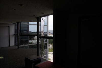
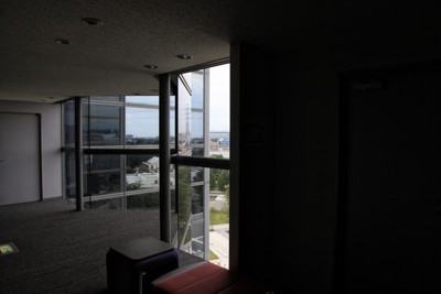
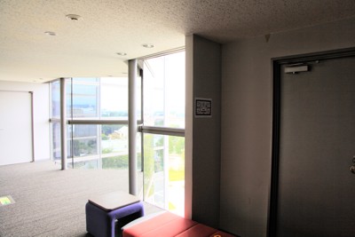
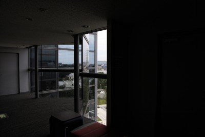
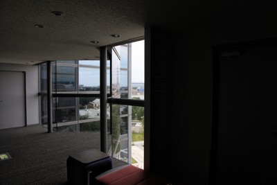
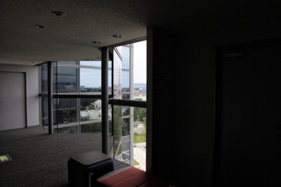
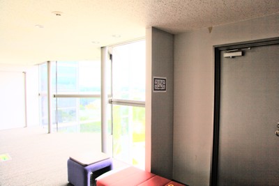
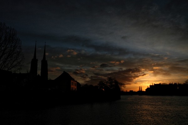
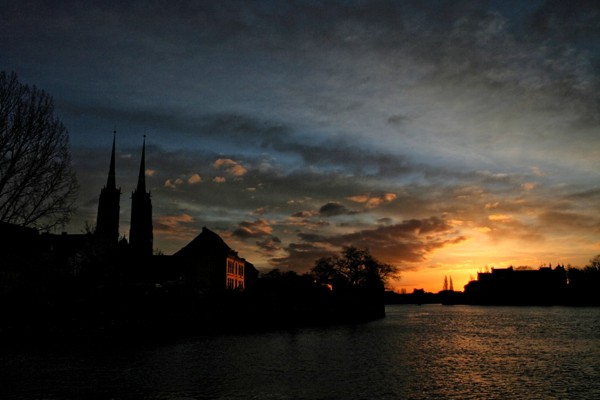
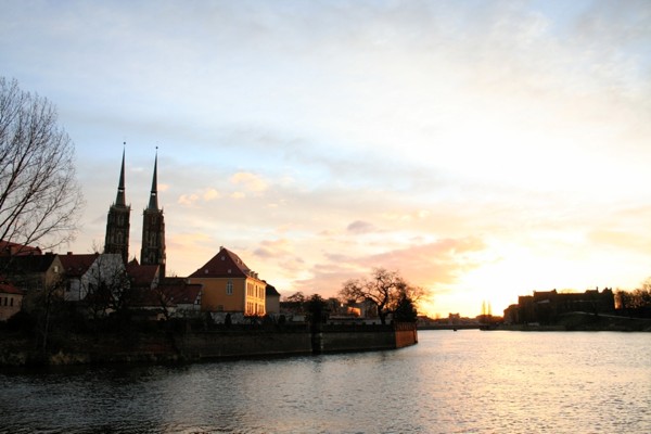
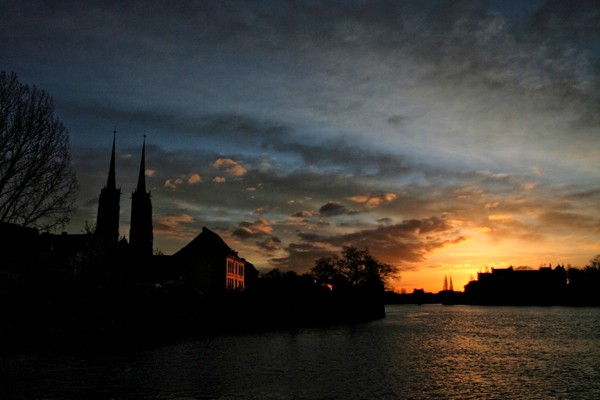
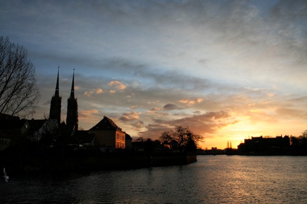
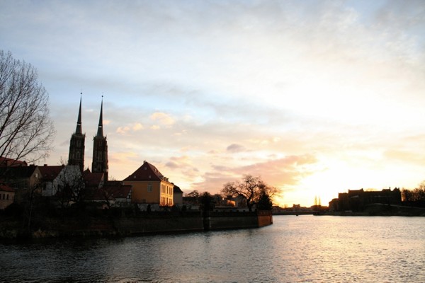
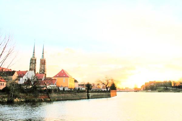
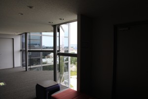
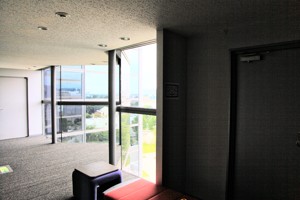
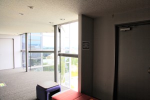
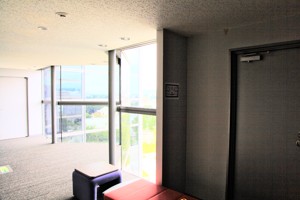
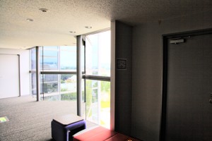
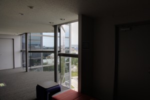
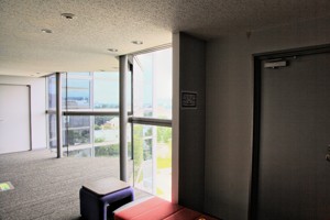
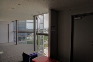
Here, we demonstrate that adjusting the luminance of unclear multi-exposure images affects the quality of the final fused images. Figures 1 and 2 show examples of adjusted multi-exposure images and fused images from these multi-exposure ones, respectively. These results indicate that adjusting the luminance makes it possible to improve the quality of fused images. In other words, even when appropriate exposure values are unknown at the time of photographing, the multi-exposure images can be improved by adjusting unclear input images. The quality of multi-exposure images depends on the degree of adjustment.
Thus, we propose a novel luminance adjustment method, referred to as “scene segmentation-based luminance adjustment” (SSLA), for multi-exposure image fusion.



III Proposed scene-segmentation-based luminance adjustment
The proposed luminance adjustment method consists of three operations: local contrast enhancement, scene segmentation-based luminance scaling (SSLS), and tone mapping (see Fig. 3). An overview of the proposed method is first described, and SSLS is then explained.
III-A Notation
The following notations are used throughout this paper.
-
•
Lower case bold italic letters, e.g., , denote vectors or vector-valued functions and are assumed to be column vectors.
-
•
A superscript denotes the transpose of a matrix or vector.
-
•
The notation denotes a -dimensional row vector.
-
•
The notation denotes a set with elements. In situations where there is no ambiguity as to their elements, the simplified notation is used to denote the same set.
-
•
The notation denotes a probability density function of .
-
•
and are used to denote the width and height of input images, respectively.
-
•
denotes a set of all pixels, namely, .
-
•
A pixel is written as .
-
•
The number of input images is denoted by .
-
•
An input image is denoted by a vector-valued function , where its output means linear-RGB pixel values, namely, the RGB color space has a linear relationship with the CIE XYZ color space. Similarly, a fused image is denoted by . For example, linear-RGB pixel values are obtained by applying the inverse gamma correction to sRGB pixel values [35]
-
•
The luminance of an image is denoted by the function , where its output corresponds to Y components of the CIE XYZ color space.
III-B Overview
The use of the proposed method in multi-exposure image fusion is illustrated in Fig. 3, where the main contributions of this paper are SSLS and the way of producing adjusted images . To enhance the quality of multi-exposure images, local contrast enhancement is applied to luminance calculated from the -th input image . Next, SSLS separates pixel set into -areas according to luminance values, and luminance for each area is then obtained by scaling a set, , of the enhanced luminance. Here, the number of the scaled luminance, which equals the number of adjusted multi-exposure images, is generally different from the number of input images. In addition, tone mapping is applied to each scaled luminance in order to avoid the truncation of pixel values. The adjusted images are generated by combining the mapped luminance and the input images , and the resulting image is then fused from these adjusted ones , by using a multi-exposure image fusion method such as weighted average.
In Fig. 3, the proposed luminance adjustment should be applied before fusion. If the luminance adjustment is applied after fusion, an additional fusion process is needed because the luminance adjustment generates multi-exposure images even when a single image is given as an input.

III-B1 Local contrast enhancement
If the input images do not represent a scene clearly, their contrast is lower than that of ideally exposed images. Therefore, the dodging and burning algorithm is used to enhance the local contrast[36]. The luminance enhanced by the algorithm is given by
| (1) |
where is the local average of luminance around pixel . It is obtained by applying a low-pass filter to . Here, a bilateral filter is used for this purpose.
III-B2 Tone mapping
Because the scaled luminance value often exceeds the maximum value of the common image formats, pixel values might be lost due to truncation of the values. This problem is overcome by using a tone mapping operation to fit the adjusted luminance value into the interval .
The luminance of an adjusted multi-exposure image is obtained by applying a tone mapping operator to :
| (4) |
Reinhard’s global operator is used here as the tone mapping operator [19].
Reinhard’s global operator is given by
| (5) |
where parameter determines value to be . Note that Reinhard’s global operator is a monotonically increasing function. Here, setting as for each , we obtain for all . Therefore, truncation of the luminance values can be prevented. In contrast, if it is preferable not to change luminance by tone mapping, setting as is chosen. As described above, each of these two parameter settings has advantages and disadvantages. In this paper, parameter is utilized.
III-B3 Fusion of enhanced multi-exposure images
III-C Scene segmentation-based luminance scaling
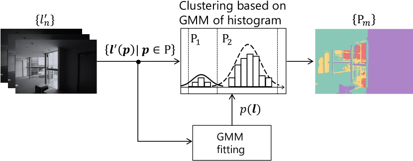
The proposed SSLS is applied to the set after local contrast enhancement as shown in Fig. 3. The purpose of SSLS is to produce luminance , which clearly represents area having a specific brightness range in a scene. For this purpose, we introduce two processes: scene segmentation and luminance scaling (see Fig. 4). In the former, the set of all pixels is divided into subsets . A set of luminance is produced in the latter process, so that luminance clearly represents area . In the latter process, luminance scaling is applied to all luminance values on , not on . This enables us to have the same image structure as before the scaling.



III-C1 Scene segmentation
Here, we discuss how to separate a scene in multi-exposure images into areas , where each has a specific brightness and . This operation is regarded as image segmentation based on luminance values. This segmentation for multi-exposure image fusion differs from typical segmentation problems such as semantic segmentation [38, 39] in two ways.
-
•
Multiple input images are given.
-
•
Attention to the structure of images, e.g., edges, is not needed.
We propose two approaches to segmentation. The first approach (Approach 1), which has low computational cost, separates a scene in multi-exposure images, according to the luminance values of an input image having middle brightness. In the second approach (Approach 2), which provides high-quality results, the scene is separated by considering the luminance distribution of all input images.
Approach 1: Let be the luminance having the middle brightness in the set . The overexposed (or underexposed) areas in are smaller than those in the other luminance images in . Namely, has the best quality in . We thus utilize to separate a scene.
In Approach 1, are given by dividing the luminance range of into equal parts:
| (7) |
where is calculated as
| (8) |
Approach 1 is very simple but is effective for most of the images shown later.
Approach 2: Approach 2 takes into account the luminance distribution of all input images, while Approach 1 only uses one of the input images for segmentation. This enables us to produce a high-quality fused image, , even when Approach 1 does not work well. A Gaussian mixture distribution is utilized to model the luminance distribution of the input images. After that, pixels are classified by using a clustering algorithm based on a Gaussian mixture model (GMM) [40].
To obtain a model considering the luminance values of all input images, we regard luminance values at a pixel as an -dimensional vector . Then the distribution of is modeled by using a GMM as
| (9) |
where is the number of mixture components, is a mixing coefficient, and is an -dimensional Gaussian distribution with mean and variance-covariance matrix .
To fit the GMM into a given , variational Bayesian inference [40] is utilized. Compared with the traditional maximum likelihood estimation, one of the advantages is that variational Bayesian inference can avoid overfitting even when we choose a large . For this reason, unnecessary mixture components are automatically removed by using the inference together with a large . is used in this paper as the maximum of the partition number .
Let us introduce a -dimensional binary random variable, , having a 1-of- representation in which a particular element is equal to 1 and all other elements are equal to 0. The values of therefore satisfy and . The marginal distribution over is specified in terms of a mixing coefficient, , such that
| (10) |
In order for to be a valid probability, must satisfy
| (11) |
together with
| (12) |
An area containing a pixel is determined by the responsibility , which is given as the conditional probability:
| (13) |
When a pixel is given and satisfies
| (14) |
the pixel is assigned to a subset of .
III-C2 Luminance scaling
The scaled luminance is simply obtained by
| (15) |
where parameter indicates the degree of adjustment (see Appendix A).
Given as a subset of , the approximate brightness of is calculated as the geometric mean of luminance values on . We thus estimate an adjusted multi-exposure image so that the geometric mean of its luminance equals the middle-gray of the displayed image, or 0.18 on a scale from zero to one, as in [19].
The geometric mean of luminance on pixel set is calculated by using
| (16) |
where is set to a small value to avoid singularities at .
III-D Combining adjusted luminance and input images
Adjusted images are obtained by combining a set of luminance adjusted by the SSLA and input multi-exposure images . To associate each with an input image , eq. (18) is utilized. As a result, combining , the -th input image , and its luminance , we obtain adjusted multi-exposure images :
| (19) |
This transformation can preserve original colors since the RGB color space has a linear relationship with the XYZ color space (see Appendix B).
III-E Proposed procedure
The procedure for generating an image from input images with the proposed method is summarized as follows (see Fig. 3).
-
i
Calculate the luminance from each input image .
- ii
- iii
- iv
- v
-
vi
Generate according to eq. (19).
-
vii
Obtain an image with a multi-exposure image fusion method as in eq. (6).
Note that the difference between Approach 1 and Approach 2 is only in step iii, and the number of satisfies . Tunable parameters in the proposed method are shown in Table I.
| Parameter | Effect |
|---|---|
| and | Determine the degree of enhancing local contrast, but larger values often boost noise or ringing. |
| Determine the shape of tone mapping operators: increases contrast, keeps all luminance values, and suppresses contrast. | |
| and | Determine the number of adjusted multi-exposure images. Larger improves the quality of fused images, but increases computational cost. In Approach 2, is automatically set such that . |
IV Simulation
We evaluated the effectiveness of the proposed SSLA in terms of the quality of fused images .
IV-A Simulation conditions
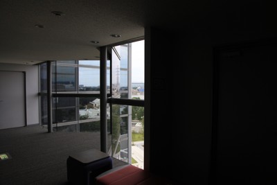
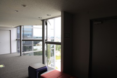
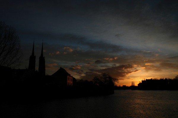
In the simulation, 20 sets of photographs and 550 sets of tone-mapped images were used as input images . Among the sets of photographs, four were taken with a Canon EOS 5D Mark II camera, and eight were selected from an available online database [41], where each set contained three multi-exposure images that were exposed with negative, zero, and positive exposure values. (see Figs. 5 and 6). The other sets were collected from database [42], where each set included moving objects. The sets of tone-mapped images were generated by tone-mapping 50 HDR images selected from online databases [43, 44]. From each HDR image, 11 sets of images were generated by linear response functions, where the number of images in ten sets was randomly decided in the range of and their exposure values were also randomly determined in the range of , to produce unclear multi-exposure images. The other set contained multi-exposure images whose exposure values were , and .



The following procedure was carried out to evaluate the effectiveness of the proposed method.
-
i
Produce from by using the proposed method.
-
ii
Obtain fused from with .
-
iii
Compute scores of three objective quality metrics: MEF-SSIM, discrete entropy and TMQI, for , as described later.
Here, we used five fusion methods for : Mertens’s method [9], Sakai’s method [14], Nejati’s method [15], Li’s method [17], and Ma’s method [32]. In Approach 1, was set so as to be the same as the number of input images. In Approach 2, was a number that satisfies , and the number was determined by the resulting GMM for each scene. The fitting of a GMM was cut off when the number of iterations reached 100, regardless of parameter convergence. In addition, Approach 2 was applied to downsized versions of for fast calculation. In particular, the resized width and height ( and , respectively) of were determined so that .
IV-B Visual evaluation
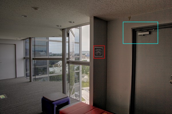
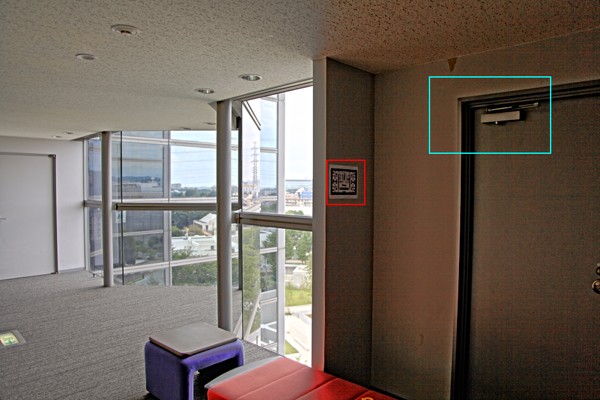
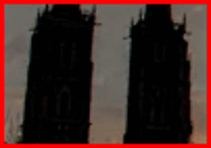
Figures 7 and 8 show images fused with/without the proposed SSLA from the input multi-exposure ones illustrated in Fig. 5. Figures. 7(7(a)) to (7(c)), Fig. 8(8(a)), and Fig. 8(8(b)) show that the effects of all of the fusion methods without luminance adjustment were not sufficient enough to visualize shadow areas when unclear input images were used as inputs. In contrast, images fused by using the proposed SSLA clearly represent the shadow areas while maintaining the quality of bright areas [see Figs. 7(7(d)) to (7(i)) and Figs. 8(8(c)) to (8(f))]. However, combining the proposed SSLA with Li’s method caused luminance inversion between bright and dark areas. Note that the inversion did not occur when Nejati’s and Ma’s methods, which are state-of-the-arts, were combined. The results for another image set in Fig. 6 are also displayed in Fig. 9. Figure 9 shows a similar trend as in Fig. 7. Therefore, the proposed SSLA makes it possible to improve the quality of fused images even when input multi-exposure images are unclear.
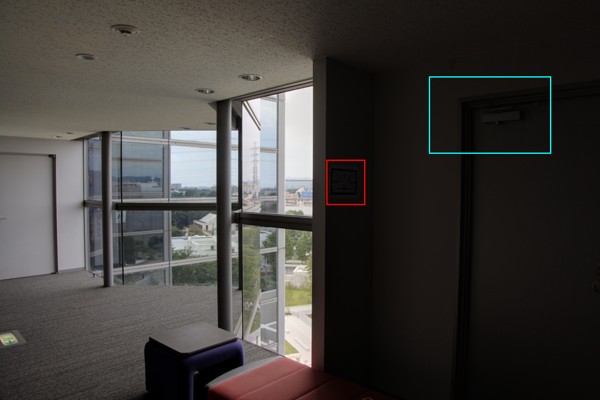
and Naturalness: 0.0569.


and Naturalness: 0.0615.
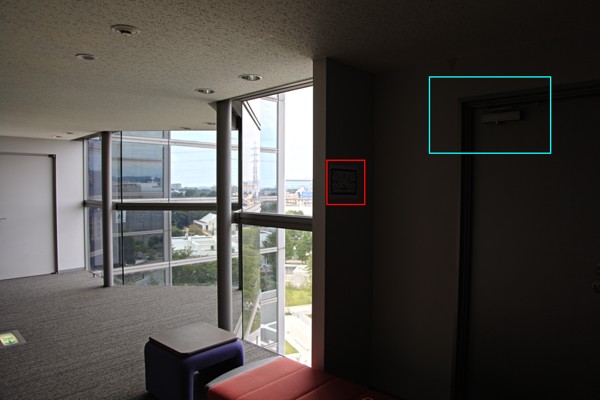
and Naturalness: 0.1617.



and Naturalness: 0.2145.
and Naturalness: 0.1655.
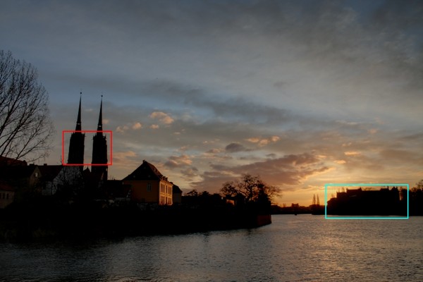
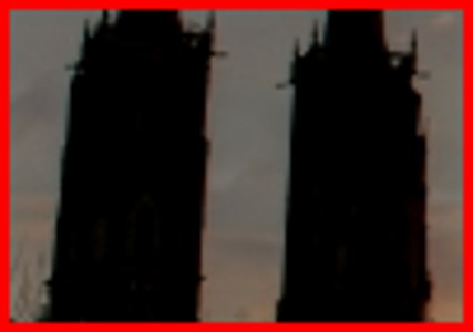

and Naturalness: 0.1445.


and Naturalness: 0.1580.
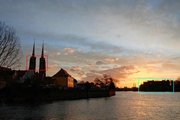
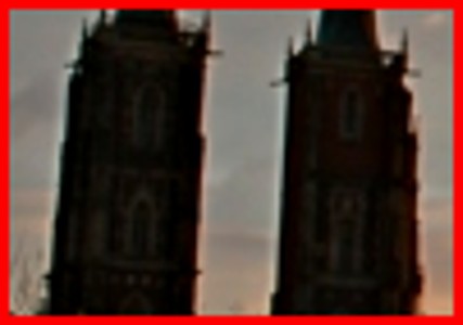
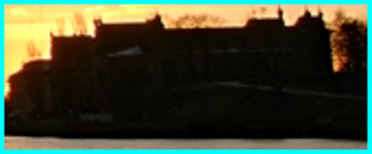
and Naturalness: 0.5090.

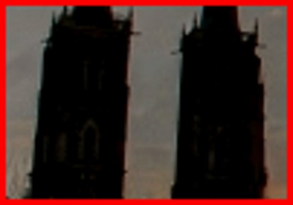
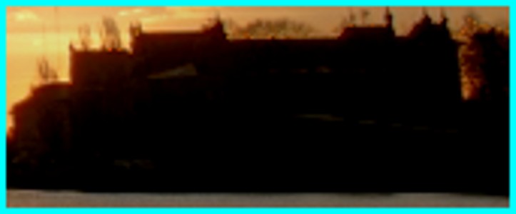
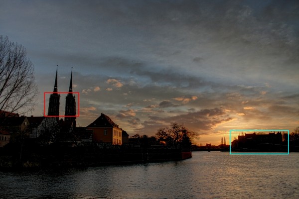

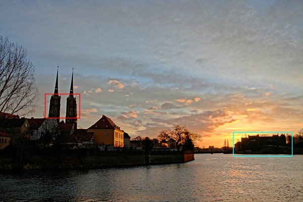

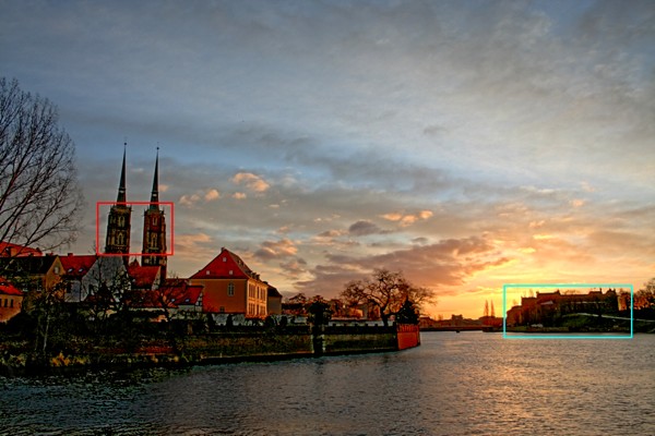
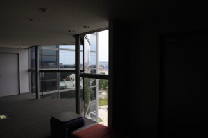
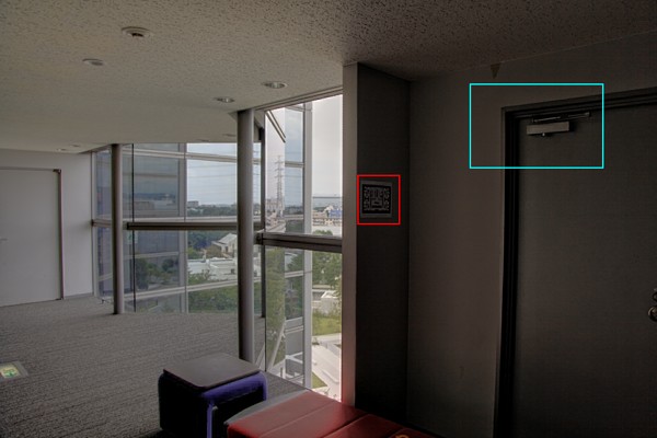
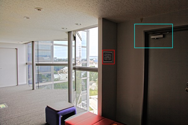
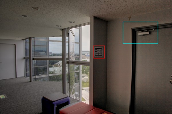
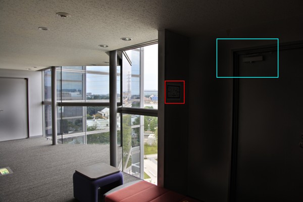
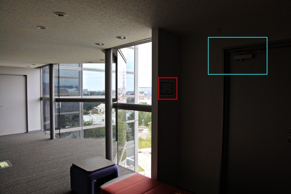
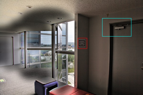
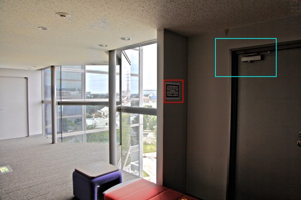
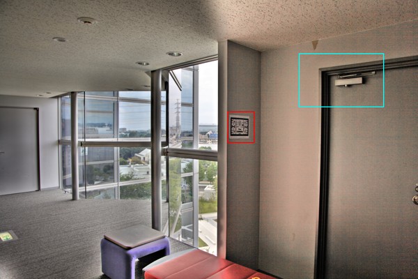
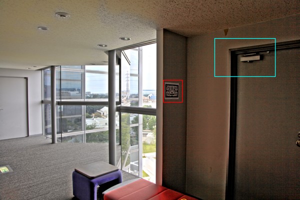
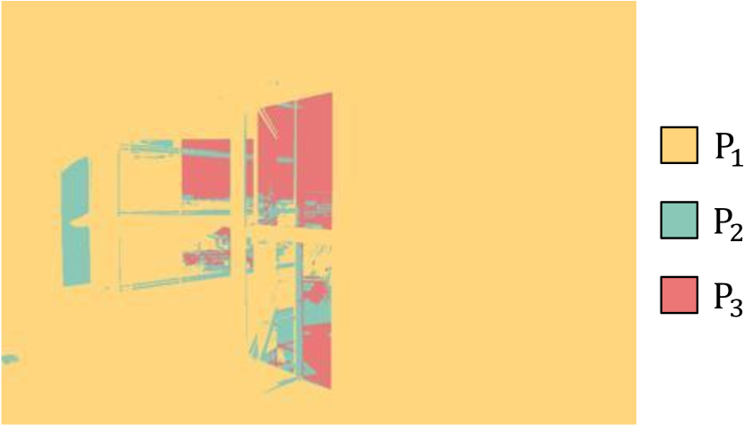
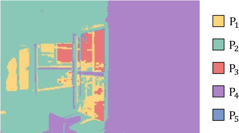
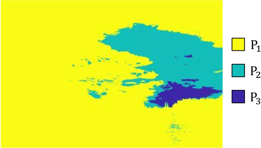
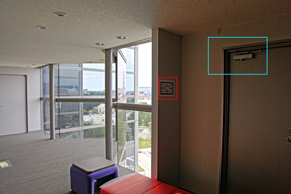
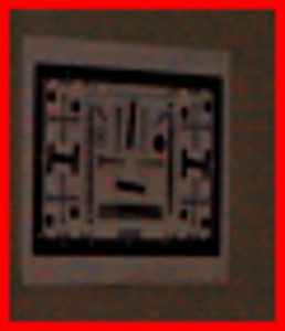
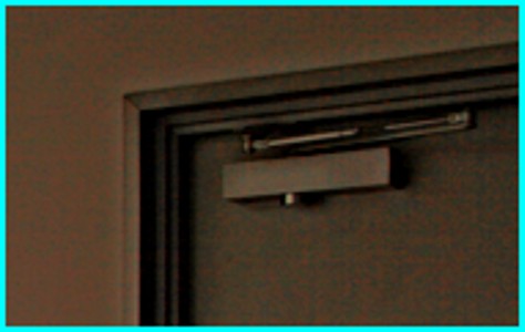
By comparing Approach 1 with Approach 2, Approach 2 generated images representing dark areas more distinctly, as shown in Figs. 7 and 9. The difference between the two approaches originates in segmented areas . Figures 10 and 11 show areas separated by Approaches 1 and 2 and adjusted multi-exposure images based on each . From Fig. 10(10(a)), it is shown that Approach 1 was not able to separate the dark areas on the right, e.g., the door, and the areas on the left with middle-brightness, e.g., the floor, while it does low computational cost. For this reason, the brightest image in Fig. 10(10(c)) does not have sufficient brightness to clearly represent the darkest areas in the scene. In comparison, Approach 2 was able to separate scenes into appropriate areas, each having a specific luminance range, even though a large was given. Figure 11 shows almost the same result as Fig. 10. Hence, it is verified that Approach 2 can separate scenes with higher accuracy than Approach 1, while Approach 1 can be performed with closed-form calculation.
Approach 1 ()
Approach 2 ()
Approach 1 ()
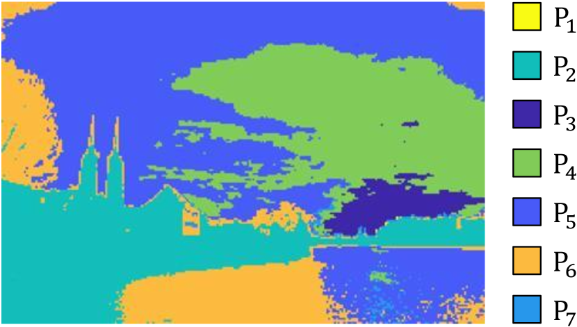
Approach 2 ()
Figures 10 and 11 also illustrate that both Approach 1 and 2 maintained the structure of images even though the two approaches did not pay attention to the structure. This result represents that the segmentation method in the proposed SSLA does not require the information of image structure such as edges. Figure 12 shows the effect of local contrast enhancement in the proposed method. This enhancement can reduce blurring and make the structure in images clear, but it often causes noise and ringing to be boosted. In this case, the proposed method without local contrast enhancement is effective to suppress such noise boosting.


Entropy: 6.848 and Naturalness: 0.7031.
Entropy: 6.810 and Naturalness: 0.5943.
Fused images from input multi-exposure ones containing moving objects are shown in Fig. 13. Even when moving objects are included in input images, the proposed method can still provide high-quality fused images without ghost-like artifacts by using a robust method to deal with dynamic scenes as fusion method . In contrast, the image generated without the proposed method contained a few ghost-like artifacts. This result indicates that the proposed method is able not only to clarify fused images, but also to remove ghost-like artifacts.
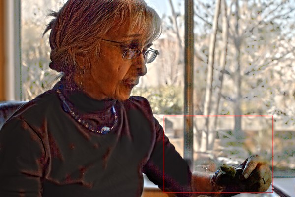
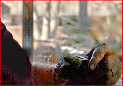
and Naturalness: 0.8262.
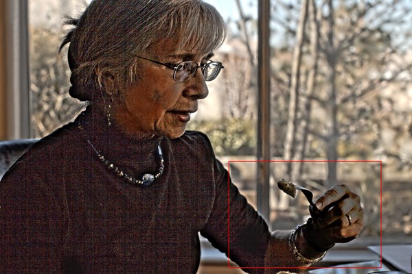
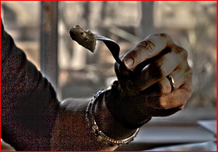
and Naturalness: 0.6731.
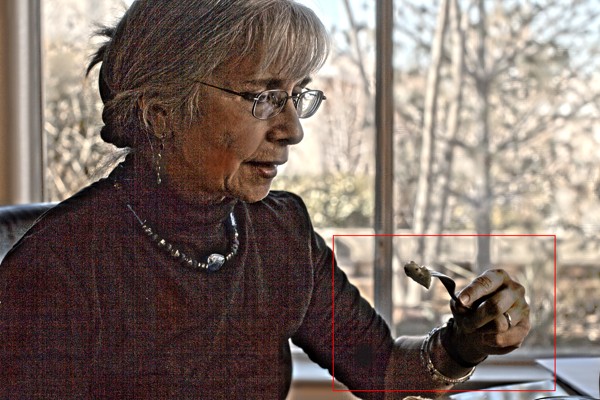
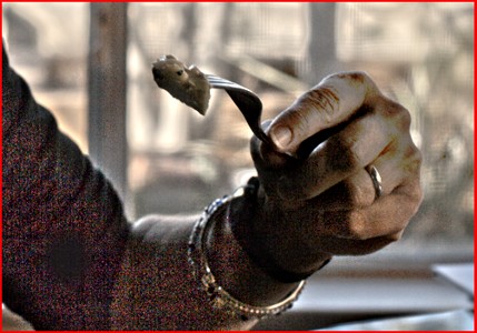
and Naturalness: 0.9701.
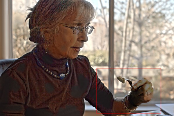
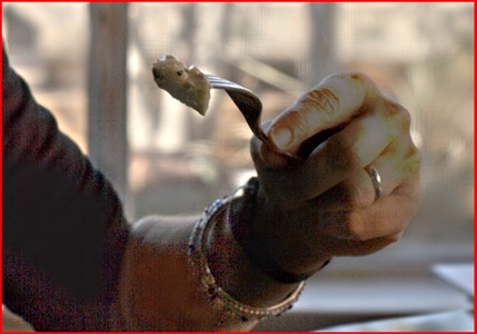
Entropy: 7.000
and Naturalness: 0.7076.
IV-C Quantitative evaluation
To quantitatively evaluate the quality of fused images, objective quality metrics are needed. Typical quality metrics such as the peak signal to noise ratio (PSNR) and structural similarity index (SSIM) are not suitable for this purpose because they use a target image with the highest quality as a reference. Recently, some full-reference metrics for multi-exposure image fusion have been proposed [45, 46]. However, because high-quality multi-exposure images are needed for these metrics, they are also not suitable for evaluating the proposed method when the multi-exposure ones are unavailable. We therefore used the metric [45], referred to as MEF-SSIM, only when high-quality multi-exposure ones are available. In other cases, the discrete entropy of luminance values and tone mapped image quality index (TMQI) [47] were used as quality metrics.
MEF-SSIM is based on a multi-scale SSIM framework and a patch consistency measure. It keeps a good balance between local structure preservation and global luminance consistency. Discrete entropy represents the amount of information in an image, where the entropy is calculated by using the luminance values of a fused image . Discrete entropy of luminance also shows the global contrast of an image. TMQI represents the quality of an image tone-mapped from an HDR image; the metric incorporates structural fidelity and statistical naturalness. Statistical naturalness [47] is defined as
| (20) |
where is a normalization factor, is a beta probability density function with parameters and , is the average luminance of an image on a scale , and is the average of local standard deviation of luminance on the scale. The Gaussian and beta distributions reflect naturalness of the global brightness and local contrast, respectively. Statistical naturalness is calculated without any reference images, although structural fidelity needs an HDR image as a reference. Since the processes of tone mapping and photographing are similar, TMQI is also useful for evaluating photographs. In this simulation, MEF-SSIM and TMQI were used only for evaluation with the sets of tone-mapped images, while discrete entropy and statistical naturalness were used for evaluation with all of the 570 sets of images.
Tables II and III summarize scores for the 12 sets of photographs of static scenes in terms of discrete entropy and statistical naturalness. For each score (discrete entropy and statistical naturalness ), a larger value means higher quality. Table II shows that the proposed SSLA provided high entropy scores for all 12 image sets, although the typical fusion methods provided low entropy scores for “Corridor 1” and “Lobby.” In addition, the proposed SSLA provided higher average scores than the typical fusion methods. Table III denotes that the proposed SSLA enables us to produce high-quality images in terms of statistical naturalness in almost all cases, compared with the typical methods.
| Scene | Mertens [9] | Sakai [14] | Nejati [15] | Li [17] | Ma [32] | ||||||||||
|---|---|---|---|---|---|---|---|---|---|---|---|---|---|---|---|
| w/o | Prop. 1 | Prop. 2 | w/o | Prop. 1 | Prop. 2 | w/o | Prop. 1 | Prop. 2 | w/o | Prop. 1 | Prop. 2 | w/o | Prop. 1 | Prop. 2 | |
| Arno | 5.987 | 5.931 | 5.833 | 5.992 | 5.935 | 5.844 | 7.016 | 7.016 | 6.793 | 6.312 | 6.095 | 6.072 | 7.054 | 7.100 | 6.813 |
| Cave | 4.938 | 5.920 | 6.277 | 4.946 | 5.942 | 6.290 | 6.132 | 6.839 | 7.044 | 6.115 | 6.840 | 6.999 | 6.082 | 6.782 | 7.043 |
| Chinese garden | 6.142 | 6.185 | 6.241 | 6.155 | 6.205 | 6.258 | 6.946 | 7.215 | 6.844 | 7.244 | 7.271 | 7.229 | 6.998 | 7.143 | 6.955 |
| Corridor 1 | 2.858 | 5.840 | 5.738 | 2.856 | 5.859 | 5.752 | 2.752 | 7.134 | 6.976 | 3.350 | 7.242 | 7.262 | 2.773 | 7.088 | 7.016 |
| Corridor 2 | 5.706 | 5.922 | 5.613 | 5.714 | 5.933 | 5.618 | 6.543 | 6.925 | 6.625 | 6.682 | 5.548 | 5.670 | 6.533 | 6.930 | 6.586 |
| Estate rsa | 6.577 | 6.604 | 6.585 | 6.560 | 6.584 | 6.573 | 6.785 | 6.917 | 7.014 | 7.001 | 7.015 | 6.914 | 6.802 | 6.921 | 7.014 |
| Kluki | 7.120 | 6.982 | 6.942 | 7.136 | 7.003 | 6.964 | 7.489 | 7.178 | 7.151 | 7.669 | 7.540 | 7.548 | 7.535 | 7.266 | 7.207 |
| Laurenziana | 6.672 | 6.478 | 6.599 | 6.678 | 6.490 | 6.609 | 7.153 | 6.956 | 6.898 | 7.585 | 7.239 | 7.417 | 7.267 | 7.091 | 7.008 |
| Lobby | 4.172 | 5.648 | 5.737 | 4.177 | 5.672 | 5.743 | 4.929 | 7.118 | 6.836 | 5.274 | 6.773 | 7.177 | 4.893 | 7.060 | 6.783 |
| Mountains | 6.920 | 6.480 | 6.571 | 6.912 | 6.492 | 6.586 | 6.823 | 6.790 | 6.846 | 6.491 | 6.233 | 6.339 | 6.796 | 6.781 | 6.838 |
| Ostrow tumski | 5.861 | 5.607 | 6.003 | 5.874 | 5.629 | 6.033 | 6.812 | 6.475 | 7.005 | 6.607 | 6.253 | 6.794 | 6.857 | 6.622 | 6.958 |
| Window | 5.047 | 5.715 | 6.060 | 5.052 | 5.735 | 6.072 | 5.407 | 6.750 | 6.848 | 5.547 | 6.617 | 7.099 | 5.402 | 6.752 | 6.868 |
| \hdashlineAverage | 5.667 | 6.109 | 6.183 | 5.671 | 6.123 | 6.195 | 6.232 | 6.943 | 6.907 | 6.323 | 6.722 | 6.877 | 6.249 | 6.961 | 6.924 |
| Scene | Mertens [9] | Sakai [14] | Nejati [15] | Li [17] | Ma [32] | ||||||||||
|---|---|---|---|---|---|---|---|---|---|---|---|---|---|---|---|
| w/o | Prop. 1 | Prop. 2 | w/o | Prop. 1 | Prop. 2 | w/o | Prop. 1 | Prop. 2 | w/o | Prop. 1 | Prop. 2 | w/o | Prop. 1 | Prop. 2 | |
| Arno | 0.1289 | 0.1382 | 0.1233 | 0.1506 | 0.1633 | 0.1473 | 0.5164 | 0.5372 | 0.5442 | 0.4079 | 0.2852 | 0.3543 | 0.5076 | 0.6845 | 0.5851 |
| Cave | 0.0758 | 0.2458 | 0.2808 | 0.0758 | 0.2236 | 0.2512 | 0.4223 | 0.3413 | 0.0628 | 0.2665 | 0.2230 | 0.0347 | 0.4122 | 0.3261 | 0.0758 |
| Chinese garden | 0.420 | 0.4353 | 0.4612 | 0.4059 | 0.4222 | 0.4441 | 0.4609 | 0.4843 | 0.4152 | 0.4801 | 0.5316 | 0.4477 | 0.4771 | 0.4468 | 0.3863 |
| Corridor 1 | 0.0004 | 0.1454 | 0.1374 | 0.0004 | 0.1998 | 0.1713 | 0.0006 | 0.9111 | 0.8792 | 0.0012 | 0.9017 | 0.9129 | 0.0006 | 0.8908 | 0.8825 |
| Corridor 2 | 0.0628 | 0.1025 | 0.0744 | 0.0763 | 0.1338 | 0.0911 | 0.3368 | 0.5052 | 0.4459 | 0.3807 | 0.0957 | 0.1293 | 0.3212 | 0.5209 | 0.4632 |
| Estate rsa | 0.7919 | 0.8047 | 0.7992 | 0.7624 | 0.7755 | 0.7840 | 0.8884 | 0.9504 | 0.9872 | 0.9773 | 0.9894 | 0.9941 | 0.9006 | 0.9536 | 0.9903 |
| Kluki | 0.9665 | 0.9580 | 0.9105 | 0.9596 | 0.9432 | 0.8889 | 0.9316 | 0.9844 | 0.9749 | 0.5148 | 0.7616 | 0.7226 | 0.8659 | 0.9849 | 0.9940 |
| Laurenziana | 0.8046 | 0.6541 | 0.7387 | 0.8058 | 0.6595 | 0.7366 | 0.9330 | 0.9722 | 0.9558 | 0.6125 | 0.9408 | 0.8303 | 0.8902 | 0.9662 | 0.9319 |
| Lobby | 0.0167 | 0.1947 | 0.2093 | 0.0190 | 0.2307 | 0.2274 | 0.1019 | 0.9260 | 0.7637 | 0.1350 | 0.6566 | 0.6936 | 0.1025 | 0.8888 | 0.7285 |
| Mountains | 0.3953 | 0.5582 | 0.6231 | 0.3562 | 0.5795 | 0.6353 | 0.4702 | 0.7383 | 0.7634 | 0.4852 | 0.5860 | 0.6898 | 0.4373 | 0.7459 | 0.8171 |
| Ostrow tumski | 0.1445 | 0.1347 | 0.2975 | 0.1580 | 0.1516 | 0.3274 | 0.5090 | 0.6194 | 0.7568 | 0.4874 | 0.3090 | 0.8185 | 0.5145 | 0.7585 | 0.8162 |
| Window | 0.0569 | 0.0912 | 0.2135 | 0.0615 | 0.1142 | 0.2650 | 0.1617 | 0.6187 | 0.7031 | 0.2145 | 0.5070 | 0.8770 | 0.1655 | 0.6413 | 0.7475 |
| \hdashlineAverage | 0.3220 | 0.3719 | 0.4057 | 0.3193 | 0.3831 | 0.4141 | 0.4777 | 0.7157 | 0.6877 | 0.4136 | 0.5657 | 0.6254 | 0.4663 | 0.734 | 0.7015 |
Tables IV and V denote scores for the eight sets of photographs of dynamic scenes in terms of discrete entropy and statistical naturalness. Here, Ma’s method was used as fusion method . Since the sets contained enough number of multi-exposure images, the scores did not have a large difference between with/without the proposed method.
| Scene | w/o | Prop. 1 | Prop. 2 | Prop. 2 w/o CE |
|---|---|---|---|---|
| Baby at window | 7.032 | 6.351 | 7.160 | 6.770 |
| Baby on grass | 7.072 | 6.711 | 7.271 | 6.966 |
| Christmas rider | 7.098 | 6.366 | 7.048 | 6.945 |
| Feeding time | 6.498 | 6.853 | 6.643 | 6.621 |
| High chair | 7.272 | 6.861 | 7.163 | 7.149 |
| Lady eating | 6.917 | 6.653 | 7.157 | 7.000 |
| Piano man | 6.633 | 6.632 | 6.791 | 6.752 |
| Santas little helper | 7.186 | 6.429 | 7.246 | 7.285 |
| \hdashlineAverage | 6.964 | 6.607 | 7.060 | 6.936 |
| Scene | w/o | Prop. 1 | Prop. 2 | Prop. 2 w/o CE |
|---|---|---|---|---|
| Baby at window | 0.9912 | 0.5344 | 0.9830 | 0.9438 |
| Baby on grass | 0.9779 | 0.6881 | 0.8532 | 0.8629 |
| Christmas rider | 0.8797 | 0.5972 | 0.7192 | 0.9593 |
| Feeding time | 0.1699 | 0.7162 | 0.6393 | 0.2859 |
| High chair | 0.9549 | 0.6721 | 0.7856 | 0.8372 |
| Lady eating | 0.8262 | 0.6731 | 0.9701 | 0.7076 |
| Piano man | 0.6369 | 0.6016 | 0.2942 | 0.7637 |
| Santas little helper | 0.6302 | 0.3866 | 0.3271 | 0.9089 |
| \hdashlineAverage | 0.7584 | 0.6087 | 0.6965 | 0.7837 |
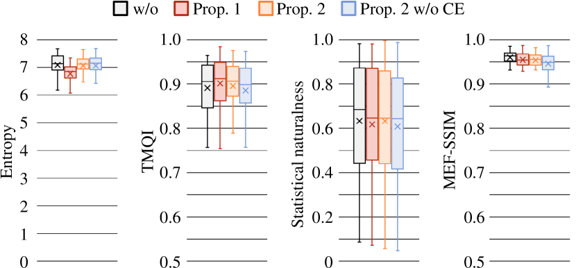
Figure 14 summarizes quantitative evaluation results for the 500 sets of unclear tone-mapped images in terms of discrete entropy, TMQI, statistical naturalness, and MEF-SSIM as box plots. The boxes span from the first to the third quartile, referred to as and , and the whiskers show the maximum and minimum values in the range of . The band inside the boxes indicates the median, i.e., the second quartile , and the crosses denote the average value. Similarly to statistical naturalness, larger TMQI and MEF-SSIM scores indicate higher quality. From this figure, it is shown that both of the approaches with the proposed method enable us to obtain images with higher-quality than images without any adjustment with any fusion method. In particular, Approach 2 provided the highest score under the use of the same fusion method in terms of all metrics. Therefore, the proposed SSLA is effective for multi-exposure image fusion when input multi-exposure images do not have a sufficient number of different exposure levels.
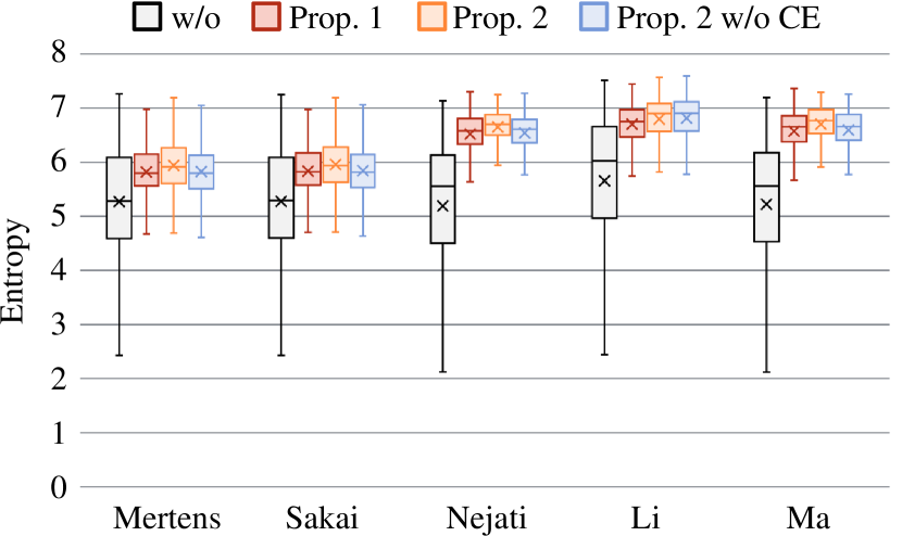
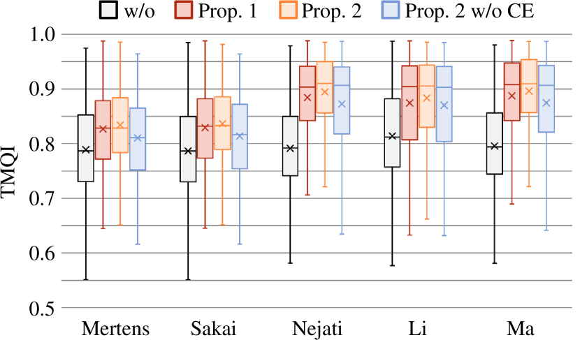
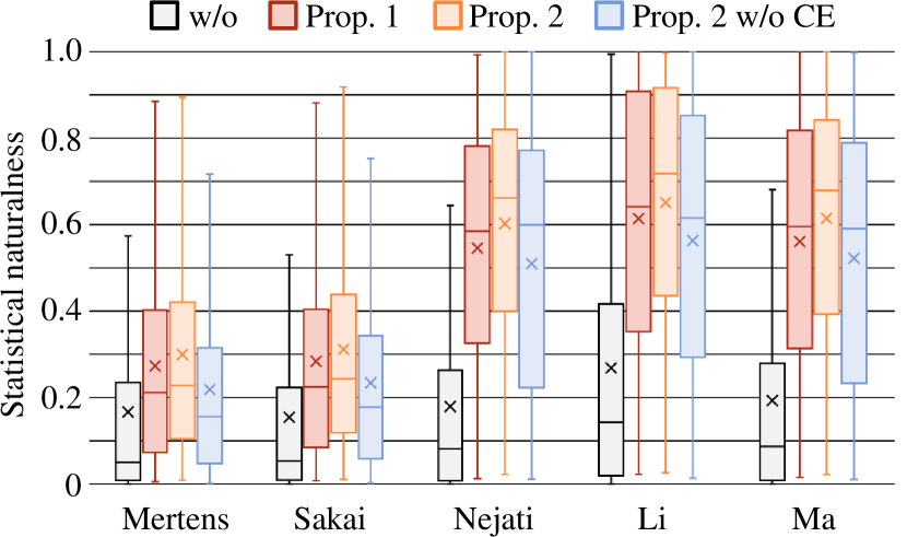
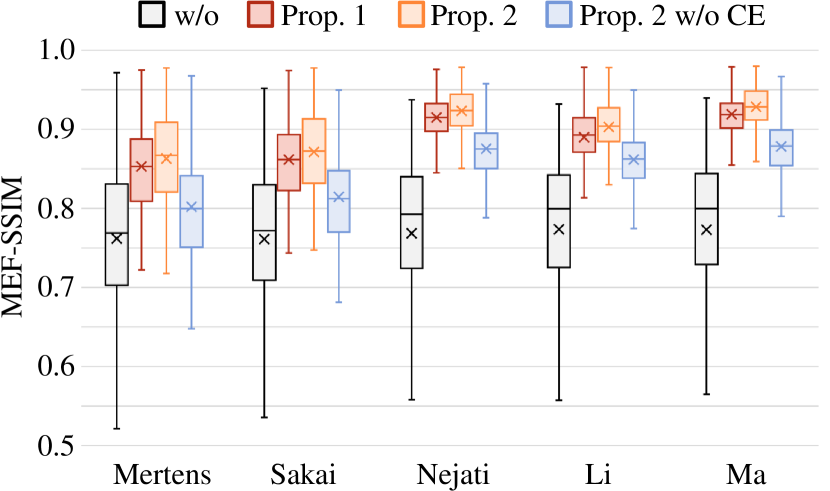
Figure 15 shows the performance of the proposed method when a sufficient number of multi-exposure images were given as inputs. Scores provided by the proposed method were almost the same as those of Ma’s method, but the scores slightly less than those of Ma’s method, Hence, it is confirmed that the proposed method does not generate a harmful effect even when well-exposed multi-exposure images are given.
For these reasons, it was confirmed that the proposed SSLA is effective for multi-exposure image fusion. It is also useful for producing high quality images that clearly represent an entire scene. Comparing Approaches 1 and 2, Approach 2 generated clear images, while Approach 1 can be performed by using a closed-form.
IV-D Computational complexity
To evaluate the computational complexity of the proposed method, we measured the executing time of the proposed one. Eight image sets selected from an available online database [41] were utilized for the evaluation. Here, the minimum and maximum number of pixels in the image sets were and , where their average was .
The simulation was run on a PC, with a 4.2 GHz processor and a main memory of 64 Gbytes (see Table VI). In the simulation, timeit() function in MATLAB was used for measuring the executing time, and every method was carried out on a single thread of execution.
| Processor | Intel Core i7-7700K 4.20 GHz |
| Memory | 64 GB |
| OS | Ubuntu 16.04 LTS |
| Software | MATLAB R2017b |
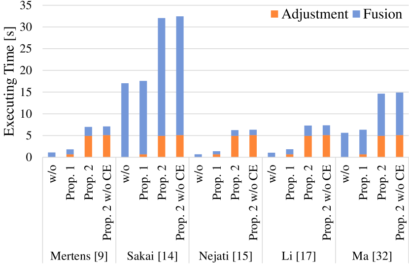
Figure 16 shows average executing time for the eight image sets. From the figure, we can see that the overhead of Approach 1 was about one second. In contrast, Approach 2 needs additional computational cost for adjustment in addition to the cost of Approach 1. Compared with Approach 1, the computational cost for fusion also increased because the number of adjusted multi-exposure images is generally larger than that of input multi-exposure images. Therefore, Approach 1 has a lower computational cost than Approach 2, while Approach 2 can generate better images than Approach 1.
V Conclusion
In this paper, we proposed a novel luminance adjustment method based on scene segmentation for multi-exposure image fusion. We first pointed out that adjusting the luminance of input images makes it possible to improve the quality of final fused images, although existing fusion methods directly fuse input multi-exposure images without any adjustment. The proposed method enables us to produce high-quality images even when undesirable inputs are given. In the method, we utilize scene segmentation in order to automatically adjust input multi-exposure images so that they become suitable for multi-exposure image fusion. For the scene segmentation, two approaches, 1 and 2, were proposed. Approach 1 separates a scene in multi-exposure images into a number of areas with closed-form calculation. In Approach 2, a scene is separated by a GMM of luminance distribution. In simulations, the proposed SSLA was applied to five fusion methods, Mertens’s one, Sakai’s one, Nejati’s one, Li’s one, and Ma’s one. The results showed that the proposed SSLA is effective with any of the fusion methods in terms of entropy and TMQI. Moreover, visual comparison results showed that the proposed SSLA makes it possible to clearly represent shadow areas in images while maintaining the quality of bright areas. In particular, Approach 2 can generate clearer images than Approach 1. The proposed SSLA was also shown to be still effective for scenes including moving objects, and ghost-like artifacts were eliminated by using the proposed SSLA with Ma’s fusion method. This indicates that the proposed SSLA is expected to improve the performance of image alignment in various image fusion problems, such as multi-exposure image fusion, HDR imaging, and panoramic image stitching. Furthermore, combining the proposed SSLA with the burst photography would enable us to improve the noise robustness.
Appendix A Relationship between exposure values and pixel values
Figure 17 shows a typical imaging pipeline for a digital camera[48]. Here, we focus on grayscale images for simplicity. The radiant power density at a sensor, i.e., irradiance , is integrated over the time that the shutter is open, producing an energy density, commonly referred to as “exposure .” If the scene is static during this integration, exposure can be written simply as the product of irradiance and integration time (referred to as “shutter speed”):
| (21) |
The photographed image is given by
| (22) |
where is a function combining sensor saturation and a camera response function (CRF). The CRF represents the processing in each camera that makes the final image look better.

Camera parameters, such as shutter speed and lens aperture, are usually calibrated in terms of exposure value (EV) units, and the proper exposure for a scene is automatically decided by the camera. The exposure value is commonly controlled by changing the shutter speed although it can also be controlled by adjusting various camera parameters. Here we assume that the camera parameters except for the shutter speed are fixed. Let and be the proper exposure value and shutter speed under the given conditions, respectively. The exposure value of an image taken at shutter speed is given by
| (23) |
From (21) to (23), images and exposed at and , respectively, are written as
| (24) | ||||
| (25) |
Assuming function is linear, we obtain a relationship between and :
| (26) |
Therefore, the exposure can be varied artificially by multiplying by a constant.
Appendix B Physical meaning of scaling RGB values
In the proposed SSLA, RGB pixel values of an adjusted multi-exposure image are given by eq. (19). Here, we prove that scaling RGB pixel values does not change colors of objects.
Let spectral distribution of illumination light striking an object, spectral reflectance of the object, and spectral response of RGB color filters on an imaging sensor as and , where means wavelength of light. Irradiance at the sensor is given as
| (27) |
From eqs. (21) and (22), RGB pixel value is written as
| (28) | ||||
| (29) |
If the radiance power of is scaled with , RGB pixel value is calculated by
| (30) | ||||
| (31) |
Assuming function is linear, namely, is a linear-RGB pixel value, we obtain a relationship between and :
| (32) |
Therefore, scaling RGB pixel value with corresponds to scaling the power of illumination light with . For this reason, scaling RGB pixel values does not change colors of objects.
Acknowledgment
This work was suppoeted by JSPS KAKENHI Grant Number JP18J20326.
References
- [1] K. Zuiderveld, “Contrast limited adaptive histogram equalization,” in Graph. gems IV, P. S. Heckbert, Ed. San Diego, CA, USA: Elsevier, 1994, pp. 474–485.
- [2] X. Wu, X. Liu, K. Hiramatsu, and K. Kashino, “Contrast-accumulated histogram equalization for image enhancement,” in Proc. IEEE Int. Conf. Imag. Process., Sep. 2017, pp. 3190–3194.
- [3] Y. Kinoshita, T. Yoshida, S. Shiota, and H. Kiya, “Pseudo multi-exposure fusion using a single image,” in Proc. Asia-Pacific Signal Inf. Process. Assoc. Annu. Summit Conf., Dec. 2017, pp. 263–269.
- [4] H. Su and C. Jung, “Low light image enhancement based on two-step noise suppression,” in Proc. IEEE Int. Conf. Acoust. Speech Signal Process., Mar. 2017, pp. 1977–1981.
- [5] X. Ren, M. Li, W.-H. Cheng, and J. Liu, “Joint enhancement and denoising method via sequential decomposition,” in Proc. IEEE Int. Symp. Circuits Syst., May. 2018, pp. 1–5.
- [6] C. Chen, Q. Chen, J. Xu, and V. Koltun, “Learning to see in the dark,” in Proc. IEEE Conf. Comput. Vis. Pattern Recognit., Jun. 2018, pp. 3291–3300.
- [7] S. W. Hasinoff, D. Sharlet, R. Geiss, A. Adams, J. T. Barron, F. Kainz, J. Chen, and M. Levoy, “Burst photography for high dynamic range and low-light imaging on mobile cameras,” ACM Trans. Graph., vol. 35, no. 6, pp. 1–12, Nov. 2016.
- [8] A. A. Goshtasby, “Fusion of multi-exposure images,” Image Vis. Comput., vol. 23, no. 6, pp. 611–618, Jun. 2005.
- [9] T. Mertens, J. Kautz, and F. Van Reeth, “Exposure fusion: a simple and practical alternative to high dynamic range photography,” Comput. Graph. Forum, vol. 28, no. 1, pp. 161–171, Mar. 2009.
- [10] A. Saleem, A. Beghdadi, and B. Boashash, “Image fusion-based contrast enhancement,” EURASIP J. Image Video Process., vol. 2012, no. 10, pp. 1–17, Dec. 2012.
- [11] S. Li and X. Kang, “Fast multi-exposure image fusion with median filter and recursive filter,” IEEE Trans. Consum. Electron., vol. 58, no. 2, pp. 626–632, May. 2012.
- [12] J. Wang, G. Xu, and H. Lou, “Exposure fusion based on sparse coding in pyramid transform domain,” in Proc. Int. Conf. Internet Multimed. Comput. Serv., Aug. 2015, pp. 1–4.
- [13] Z. Li, J. Zheng, Z. Zhu, and S. Wu, “Selectively detail-enhanced fusion of differently exposed images with moving objects,” IEEE Trans. Image Process., vol. 23, no. 10, pp. 4372–4382, Oct. 2014.
- [14] T. Sakai, D. Kimura, T. Yoshida, and M. Iwahashi, “Hybrid method for multi-exposure image fusion based on weighted mean and sparse representation,” in Proc. Eur. Signal Process. Conf., Aug. 2015, pp. 809–813.
- [15] M. Nejati, M. Karimi, S. R. Soroushmehr, N. Karimi, S. Samavi, and K. Najarian, “Fast exposure fusion using exposedness function,” in Proc. IEEE Int. Conf. Imag. Process., Sep. 2017, pp. 2234–2238.
- [16] K. R. Prabhakar, V. S. Srikar, and R. V. Babu, “DeepFuse: a deep unsupervised approach for exposure fusion with extreme exposure image pairs,” in Proc. IEEE Int. Conf. Comput. Vis., Oct. 2017, pp. 4724–4732.
- [17] Shutao Li, Xudong Kang, and Jianwen Hu, “Image fusion with guided filtering,” IEEE Trans. Image Process., vol. 22, no. 7, pp. 2864–2875, Jul. 2013.
- [18] P. E. Debevec and J. Malik, “Recovering high dynamic range radiance maps from photographs,” in Proc. Annu. Conf. Comput. Graph. Interact. Tech., Aug. 1997, pp. 369–378.
- [19] E. Reinhard, M. Stark, P. Shirley, and J. Ferwerda, “Photographic tone reproduction for digital images,” ACM Trans. Graph., vol. 21, no. 3, pp. 267–276, Jul. 2002.
- [20] T.-H. Oh, J.-Y. Lee, Y.-W. Tai, and I. S. Kweon, “Robust high dynamic range imaging by rank minimization,” IEEE Trans. Pattern Anal. Mach. Intell., vol. 37, no. 6, pp. 1219–1232, Jun. 2015.
- [21] Y. Kinoshita, S. Shiota, M. Iwahashi, and H. Kiya, “An remapping operation without tone mapping parameters for HDR images,” IEICE Trans. Fundam. Electron. Commun. Comput. Sci., vol. E99-A, no. 11, pp. 1955–1961, Nov. 2016.
- [22] Y. Kinoshita, S. Shiota, and H. Kiya, “Fast inverse tone mapping with Reinhard’s global operator,” in Proc. IEEE Int. Conf. Acoust. Speech Signal Process., Mar. 2017, pp. 1972–1976.
- [23] Y. Kinoshita, S. Shiota, and H. Kiya, “Fast inverse tone mapping based on Reinhard’s global operator with estimated parameters,” IEICE Trans. Fundam. Electron. Commun. Comput. Sci., vol. E100-A, no. 11, pp. 2248–2255, Nov. 2017.
- [24] Y. Q. Huo and X. D. Zhang, “Single image-based HDR imaging with CRF estimation,” in Proc. IEEE Int. Conf. Commun. Probl., Sep. 2016, pp. 1–3.
- [25] T. Murofushi, M. Iwahashi, and H. Kiya, “An integer tone mapping operation for HDR images expressed in floating point data,” in Proc. IEEE Int. Conf. Acoust. Speech Signal Process., May. 2013, pp. 2479–2483.
- [26] T. Murofushi, T. Dobashi, M. Iwahashi, and H. Kiya, “An integer tone mapping operation for HDR images in OpenEXR with denormalized numbers,” in Proc. IEEE Int. Conf. Imag. Process., Oct. 2014, pp. 4497–4501.
- [27] T. Dobashi, T. Murofushi, M. Iwahashi, and K. Hitoshi, “A fixed-point global tone mapping operation for HDR images in the RGBE format,” IEICE Trans. Fundam. Electron. Commun. Comput. Sci., vol. E97-A, no. 11, pp. 2147–2153, Nov. 2014.
- [28] Y. Kinoshita, S. Shiota, H. Kiya, and T. Yoshida, “Multi-exposure image fusion based on exposure compensation,” in Proc. IEEE Int. Conf. Acoust. Speech Signal Process., Apr. 2018, pp. 1388–1392.
- [29] Y. Kinoshita, S. Shiota, and H. Kiya, “Automatic exposure compensation for multi-exposure image fusion,” in Proc. IEEE Int. Conf. Imag. Process., Oct. 2018, pp. 883–887.
- [30] S. Nayar and T. Mitsunaga, “High dynamic range imaging: spatially varying pixel exposures,” in Proc. IEEE Conf. Comput. Vis. Pattern Recognit., Jun. 2000, pp. 472–479.
- [31] V. G. An and C. Lee, “Single-shot high dynamic range imaging via deep convolutional neural network,” in Proc. Asia-Pacific Signal Inf. Process. Assoc. Annu. Summit Conf., Dec. 2017, pp. 1768–1772.
- [32] K. Ma, H. Li, H. Yong, Z. Wang, D. Meng, and L. Zhang, “Robust multi-exposure image fusion: a structural patch decomposition approach,” IEEE Trans. Image Process., vol. 26, no. 5, pp. 2519–2532, May. 2017.
- [33] M. Aggarwal and N. Ahuja, “Split aperture imaging for high dynamic range,” Int. J. Comput. Vis., vol. 58, no. 1, pp. 7–17, Jun. 2004.
- [34] M. D. Tocci, C. Kiser, N. Tocci, and P. Sen, “A versatile HDR video production system,” ACM Trans. Graph., vol. 30, no. 4, pp. 41:1—-41:10, Jul. 2011.
- [35] IEC, “Multimedia systems and equipment - Colour measurement and management - Part 2-1: Colour management - Default RGB colour space - sRGB,” IEC 61966-2-1, Oct. 1999.
- [36] H. Youngquing, Y. Fan, and V. Brost, “Dodging and burning inspired inverse tone mapping algorithm,” J. Comput. Inf. Syst., vol. 9, no. 9, pp. 3461–3468, May. 2013.
- [37] J. Chen, S. Paris, and F. Durand, “Real-time edge-aware image processing with the bilateral grid,” ACM Trans. Graph., vol. 26, no. 3, p. 103, Jul. 2007.
- [38] A. Kanezaki, “Unsupervised image segmentation by backpropagation,” in Proc. IEEE Int. Conf. Acoust. Speech Signal Process., Apr. 2018, pp. 1543–1547.
- [39] L.-C. Chen, G. Papandreou, I. Kokkinos, K. Murphy, and A. L. Yuille, “DeepLab: semantic image segmentation with deep convolutional nets, atrous convolution, and fully connected CRFs,” IEEE Trans. Pattern Anal. Mach. Intell., vol. 40, no. 4, pp. 834–848, Apr. 2018.
- [40] C. M. Bishop, Pattern recognition and machine learning. New York, NY, USA: Springer-Verlag, 2006.
- [41] “HDR photography gallery.” [Online]. Available: https://www.easyhdr.com/examples/
- [42] P. Sen, N. K. Kalantari, M. Yaesoubi, S. Darabi, D. B. Goldman, and E. Shechtman, “Robust patch-based hdr reconstruction of dynamic scenes,” ACM Trans. Graph., vol. 31, no. 6, pp. 203:1—-203:11, Nov. 2012.
- [43] P. Zolliker, Z. Barańczuk, D. Küpper, I. Sprow, and T. Stamm, “Creating HDR video content for visual quality assessment using stop-motion,” in Proc. Eur. Signal Process. Conf., Sep. 2013, pp. 1–5.
- [44] “The HDR photographic survey.” [Online]. Available: http://rit-mcsl.org/fairchild/HDRPS/HDRthumbs.html
- [45] K. Ma, Kai Zeng, and Zhou Wang, “Perceptual quality assessment for multi-exposure image fusion,” IEEE Trans. Image Process., vol. 24, no. 11, pp. 3345–3356, Nov. 2015.
- [46] H. Rahman, R. Soundararajan, and R. V. Babu, “Evaluating multiexposure fusion using image information,” IEEE Signal Process. Lett., vol. 24, no. 11, pp. 1671–1675, Nov. 2017.
- [47] H. Yeganeh and Z. Wang, “Objective quality assessment of tone-mapped images,” IEEE Trans. Image Process., vol. 22, no. 2, pp. 657–667, Feb. 2013.
- [48] F. Dufaux, P. L. Callet, R. Mantiuk, and M. Mrak, High dynamic range video, from acquisition, to display and applications. Cambridge, MA, USA: Academic Press, 2016.
![[Uncaptioned image]](/html/1903.07428/assets/figs/bio_kinoshita.jpg) |
Yuma Kinoshita received his B.Eng. and M.Eng. degrees from Tokyo Metropolitan University, Japan, in 2016 and 2018, respectively. From 2018, he has been a Ph.D. student at Tokyo Metropolitan University. He received IEEE ISPACS Best Paper Award in 2016, IEEE Signal Processing Society Japan Student Conference Paper Award in 2018, and IEEE Signal Processing Society Tokyo Joint Chapter Student Award in 2018, respectively. His research interests are in the area of image processing. He is a student member of IEEE and IEICE. |
![[Uncaptioned image]](/html/1903.07428/assets/figs/bio_kiya.jpg) |
Hitoshi Kiya received his B.E and M.E. degrees from Nagaoka University of Technology, in 1980 and 1982 respectively, and his Dr. Eng. degree from Tokyo Metropolitan University in 1987. In 1982, he joined Tokyo Metropolitan University, where he became Full Professor in 2000. From 1995 to 1996, he attended the University of Sydney, Australia as a Visiting Fellow. He is a Fellow of IEEE, IEICE and ITE. He currently serves as President of APSIPA, and he served as Inaugural Vice President (Technical Activities) of APSIPA in 2009-2013, and as Regional Director-at-Large for Region 10 of IEEE Signal Processing Society in 2016-2017. He was also President of IEICE Engineering Sciences Society in 2011-2012, and he served there as Vice President and Editor-in-Chief for IEICE Society Magazine and Society Publications. He was Editorial Board Member of eight journals, including IEEE Trans. on Signal Processing, Image Processing, and Information Forensics and Security, Chair of two technical committees and Member of nine technical committees including APSIPA Image, Video, and Multimedia Technical Committee (TC), and IEEE Information Forensics and Security TC. He has organized a lot of international conferences, in such roles as TPC Chair of IEEE ICASSP 2012 and as General Co-Chair of IEEE ISCAS 2019. Dr. Kiya is a recipient of numerous awards, including six best paper awards. |
