New Pair of Primal Dual Algorithms for Bregman Iterated Variational Regularization

Abstract

Primal-dual splitting involving proximity operators in order to be able to find some approximation to the minimizer for a general form of Tikhonov type functional is in the focus of this work. This approximation is produced by a pair of iterative variational regularization procedures.

Under the assumption of some variational source condition (VSC), total error estimation both in the iterative sense and in the continuous sense has been analysed separately. Rates of convergence will be obtained in terms some concave and positive definite index function. Of the choice of the penalty term, we are interested in Bregman distance penalization associated with the non-smooth total variation (TV) functional. Furthermore, following up the lower and bounds defined for the regularization parameter, some deterministic choice of the regularization parameter is given explicitly. It is in the emphasis of this work that the regularization parameter obeys Morozov‘s discrepancy principle (MDP) in order for the stability analysis of regularized solution.

In the computerized environment, the algorithms are verified as iterative regularization methods by applying it to an atmospheric tomography problem named as GPS-Tomography. Apart from this 3-D tomographic inverse problem, we also apply the algorithms to some 2-D conventional tomographic image reconstruction problems in order to be able test algorithms‘ capability of capturing the details and observe that algorithms behave as iterative regularization procedures.

Keywords. iterative regularization, primal dual algorithm, Bregman iteration, total variation

footnote

1 Introduction

Following up a recent work in [3], we introduce the primal dual algorithms in the simpler forms without nested loops. Both algorithms are to be used for the purpose of finding iteratively regularized approximations for the inverse ill-posed problems. Stability analyses are reduced to be in the emphasis of the stability of the iteratively regularized approximations of the regularized minimizer for some general form of Tikhonov functional.

In general terms, regularization theory deals with approximation of some ill-posed inverse problem by a family of parametrized well-posed problems. Traditional quadratic-Tikhonov regularization [76, 77] has been well established and analyzed [34]. This work focuses on the analysis of some iterative regularization procedures.

Proximal mapping algorithms and Bregman iterated regularization procedures have been commonly known. Here, Bregman distance plays the role of penalization in the corresponding minimization problems. Having a look at the literature, firstly in the work [64], Bregman iteration has been proposed for providing solution to the basis pursuit problem. In a recent study by Sprung and Hohage et al., 2017, [74], authors have investigated convergence rates results for the such objective functionals with the Bregman distance as penalty term. Having optimization algorithms in the field of inverse problems as iterative regularization method has also become popular. Authors in [37] have proposed some primal-dual algorithm, wherein the convergence has been studied for the given noiseless measurement data. We consider linear, inverse ill-posed problems in the general form. Stability of the algorithms will be developed in the context of convex variational regularization and be verified in the Hadamard sense. Main results of our work are derived in the case of noisy measurement and are in the best interest of variational regularization theory.

2 Notations and Mathematical Setting

Over the finite dimensional Hilbert spaces ${\mathcal{X}}=\mathbb{R}^{N}$ and ${\mathcal{Y}}=\mathbb{R}^{M}$, let us be given some linear, injective, forward operator $T:{\mathcal{X}}\rightarrow{\mathcal{Y}}.$ In this work, we concentrate on the numerical solution for the linear inverse ill-posed problem of the form

$$\delta\xi+Tu=v^{\delta},$$ (2.1)

with some iterative regularization procedure. Here, the given noisy data $v^{\delta}\in{\mathcal{Y}}$ and the noise model is denoted by $\xi$ with the noise magnitude $\delta.$

Non-negativity constraint on our targeted data $u$ is imposed. Then, the constraint domain is treated as the indicator function $h:{\mathcal{X}}\longrightarrow\{0,1\}$ defined by

$$h(u)=1_{\Omega}(u):=\left\{\begin{array}[]{rcl}0&\mbox{, for}&u\in\Omega\subset{\mathcal{X}}\\ \infty&\mbox{, for}&u\notin\Omega\subset{\mathcal{X}}.\end{array}\right.$$ (2.2)

Throughout the work, unless otherwise stated, the notation $||\cdot||$ without any subscript will be used as to denote the usual Euclidean norm. Let $\sigma(T^{T}T)$ be the spectrum of $T^{T}T$ is the set of those $\sigma_{k}\in\mathbb{R}^{N}.$ Then, for the finite dimensional forward operator $T:\mathbb{R}^{N}\rightarrow\mathbb{R}^{M}$ where $M<N,$ we define

$$||T||:=\max_{1\leq k\leq M}\left\{\sqrt{\sigma_{k}}\right\}.$$

Below, we give two norm estimations that will be in use of our mathematical development. For some $u_{1},u_{2}\in{\mathcal{X}}$ and $\lambda\in\mathbb{R},$ the following equality holds, [75, Eq. (2.1)],

$$||\lambda u_{1}+(1-\lambda)u_{2}||^{2}=\lambda||u_{1}||^{2}+(1-\lambda)||u_{2}||^{2}-\lambda(1-\lambda)||u_{1}-u_{2}||^{2}.$$ (2.3)

Also, nonexpansiveness of the misfit term provides,

$$||T^{T}T(u_{1}-u_{2})||^{2} \leq ||T||^{2}||T(u_{1}-u_{2})||^{2}$$

$$= ||T||^{2}\langle T(u_{1}-u_{2}),T(u_{1}-u_{2})\rangle$$

$$= ||T||^{2}\langle T^{T}T(u_{1}-u_{2}),u_{1}-u_{2}\rangle,$$

which implies

$$-\langle u_{1}-u_{2},T^{T}T(u_{1}-u_{2})\rangle\leq-\frac{1}{||T||^{2}}||T^{T}T(u_{1}-u_{2})||^{2}$$ (2.4)

For some function $f:{\mathcal{X}}\rightarrow{\mathcal{Y}}$ and some point $x$ in the domain of $f,$ the subdifferential of $f$ at $x^{\prime},$ denotes $\partial f(x^{\prime})$ is defined by

$$\partial f(x^{\prime}):=\left\{\eta\in{\mathcal{X}}^{\ast}:f(x)-f(x^{\prime})\geq\langle\eta,x-x^{\prime}\rangle\mbox{ for all }x\in{\mathcal{X}}\right\}.$$ (2.5)

Definition 2.1.

[Generalized Bregman Distances] Let ${\mathcal{J}}:{\mathcal{X}}\rightarrow\mathbb{R}_{+}\cup\{\infty\}$ be a convex functional with the subgradient $q^{\ast}\in\partial{\mathcal{J}}(u^{\ast}).$ Then, for $u,u^{\ast}\in{\mathcal{X}},$ Bregman distance associated with the functional $J$ is defined by

$$D_{{\mathcal{J}}}: {\mathcal{X}}\times{\mathcal{X}} \longrightarrow\mathbb{R}_{+}$$ (2.6)

$$(u,u^{\ast}) \longmapsto D_{{\mathcal{J}}}(u,u^{\ast}):={\mathcal{J}}(u)-{\mathcal{J}}(u^{\ast})-\langle q^{\ast},u-u^{\ast}\rangle.$$

It is well known that the Bregman distance does not satisfy symmetry,

$$D_{{\mathcal{J}}}(u,u^{\ast})\neq D_{{\mathcal{J}}}(u^{\ast},u),$$

and for the defined convex functional ${\mathcal{J}}$

$$D_{{\mathcal{J}}}(u,u^{\ast})\geq 0.$$

With all these tools stated, we consider the following objective functional,

$$F_{\alpha}: {\mathcal{X}} \times{\mathcal{Y}}\longrightarrow\mathbb{R}_{+}$$ (2.7)

$$(u ,v^{\delta})\longmapsto F_{\alpha}(u,v^{\delta}):=\frac{1}{2}||Tu-v^{\delta}||^{2}+\alpha D_{{\mathcal{J}}}(u,u_{0})+h(u),$$

with some initial estimation $u_{0}\in{\mathcal{X}}.$ In particular, we associate the Bregman distance penalty term with the total variation (TV) functional defined by

$$TV(u,\Omega)={\mathcal{J}}(u):=\int_{\Omega}|\nabla u(x)|dx\approxeq\sum_{i}|\nabla_{i}u|,$$ (2.8)

which is, in 3D case, $i=(i_{x},i_{y},i_{z}).$ For the sake of following the further calculations easily in the future developments of this work, we introduce TV in the composite form

$$J(u)=g(Du)\mbox{ where, }g(\cdot)=||\cdot||_{1}\mbox{ with }D(\cdot)=\nabla(\cdot).$$ (2.9)

Thus,

$$\partial J(u)=D^{\ast}\partial g(Du).$$ (2.10)

2.1 Overview on the iterative regularization and the choice of the regularization parameter

By an iterative procedure involving some iteration operator $R_{I},$ [14, Ch. 6], we aim to construct some approximation to the given inverse ill-posed problem (2.1)

$$u_{i}=R_{I}(v^{\delta},w_{i-1},\Gamma),$$ (2.11)

where $w^{i-1}$ is the collection of dual variables used during $i-1$ iteration steps, and $\Gamma$ is the auxiliary parameters such as step-size, relaxation parameter, regularization parameter.

In the iterative regularization procedures, discrepancy principles act as the stopping rules for the corresponding algorithms, [14, Section 6].

Definition 2.2.

[Morozov‘s Discrepancy Principle (MDP), [14, Def. 6.1]]

Given deterministic noise model $||v^{\dagger}-v^{\delta}||\leq\delta,$ if we choose $\tau>1$ and $i^{\ast}=i^{\ast}(\delta,v^{\delta})$ such that

$$||Tu_{i^{\ast}}-v^{\delta}||\leq\tau\delta<||Tu_{i}-v^{\delta}||$$ (2.12)

is satisfied for $u_{i^{\ast}}=R_{I}(v^{\delta},w_{i^{\ast}-1},\vec{\alpha})$ and $u_{i}=R_{I}(v^{\delta},w_{i-1},\vec{\alpha})$ for all $i<i^{\ast},$ then $u_{i^{\ast}}$ is said to satisfy Morozov‘s discrepancy principle.

Following up MDP, some immediate consequences can be given below,

$$||Tu_{i^{\ast}}^{\delta}-Tu^{\dagger}||\leq(\tau+1)\delta,$$ (2.13)

likewise,

$$\tau\delta\leq||Tu_{i}-v^{\delta}|| \Rightarrow \tau\delta\leq||Tu_{i}-Tu^{\dagger}||+\delta$$ (2.14)

$$\Rightarrow (\tau-1)\delta\leq||Tu_{i}-Tu^{\dagger}||$$

$$\Rightarrow (\tau-1)^{2}\delta^{2}\leq||Tu_{i}-Tu^{\dagger}||^{2}$$

$$\Rightarrow -||Tu_{i}-Tu^{\dagger}||^{2}\leq-(\tau-1)^{2}\delta^{2}$$

Our primal-dual splitting algorithms involve proximal mapping that is defined below.

Definition 2.3.

[Proximal mapping] Let ${\mathcal{J}}:\mathbb{R}^{N}\rightarrow\mathbb{R}\cup\{\infty\}$ be a proper, convex, lower-semicontinious function. Then $\mathrm{prox}_{{\mathcal{J}}}$ is defined as the unique minimizer

$$\mathrm{prox}_{{\mathcal{J}}}(\tilde{u}):={\rm arg\,min}_{u\in\mathbb{R}^{N}}{\mathcal{J}}(u)+\frac{1}{2}||u-\tilde{u}||^{2}.$$

Measuring the deviation of the regularized solution $u_{\alpha}^{\delta}$ from the minimum norm solution $u^{\dagger}$ by the a priori and a posteriori strategies for the choice of the regularization parameter in Banach spaces with the VSC has been widely studied,

The objective of convergence and convergence rates results in the regularization theory is to be able find some stable bound for the total error estimation function defined by

$$E: {\mathcal{X}}\times{\mathcal{X}} \longrightarrow\mathbb{R}_{+}$$ (2.15)

$$(u_{\alpha}^{\delta},u^{\dagger}) \longrightarrow E(u_{\alpha}^{\delta},u^{\dagger}):=\Lambda||u_{\alpha}^{\delta}-u^{\dagger}||,$$

where the coefficient $\Lambda\in\mathbb{R}_{+}$ depends on the functional properties of the data on the pre-image space. Such estimation requires the knowledge of the smoothness of the minimum norm solution $u^{\dagger}$ which is some source condition in the form of varitional inequality, [15], [35], [38], [46, Eq. (1.4)], [45], [52, Section 4] [71, Theorem 2.60 - (g), Subsection 3.2.4]. Convergence and convergence rates results, or in other words the total error estimation, are derived in terms of a concave, monotonically increasing, positive definite index function that is a part of the VSC expression. Following up the work [3], the form of VSC that will be used in our analysis is given below. Also in the aforementioned works that have been dedicated to variational regularization, derivation of noise dependent error estimation following from VSC has been well explained. In our work, any data that is in the constraint domain is assumed to satisfy VSC.

Assumption 2.4.

[Variational Source Condition] Let $T:{\mathcal{X}}\rightarrow{\mathcal{Y}}$ be linear, injective forward operator and $v^{\dagger}\in\mathrm{range}(T).$ There exists some constant $\sigma\in(0,1]$ and a concave, monotonically increasing index function $\Psi$ with $\Psi(0)=0$ and $\Psi:[0,\infty)\rightarrow[0,\infty)$ such that for $q^{\dagger}\in\partial{\mathcal{J}}(u^{\dagger})$ the minimum norm solution $u^{\dagger}\in\mathrm{BV}(\Omega)$ satisfies

$$\sigma||u-u^{\dagger}||\leq{\mathcal{J}}(u)-{\mathcal{J}}(u^{\dagger})+\Psi\left(||Tu-Tu^{\dagger}||\right)\mbox{, for all }u\in{\mathcal{X}}.$$ (2.16)

3 Subdifferential Characterization

Both algorithms will evolve from the subdifferential characterization of the regularized minimizer of the objective functional (2.7). Then, by its first order optimality condition,

$$0\in\partial F_{\alpha_{\ast}}(u_{\alpha_{\ast}}^{\delta},v^{\delta}),$$

which implies,

$$0=T^{T}(Tu_{\alpha_{\ast}}^{\delta}-v^{\delta})+\alpha_{\ast}\partial{\mathcal{J}}(u_{\alpha_{\ast}}^{\delta})-\alpha_{\ast}\partial{\mathcal{J}}(u_{0})+\hat{z}\mbox{, where }\hat{z}\in\partial h(u_{\alpha_{\ast}}^{\delta}).$$ (3.1)

Furthermore, recall the settings in (2.9) and (2.10) to represent (3.1) in the following form

$$0=T^{T}(Tu_{\alpha_{\ast}}^{\delta}-v^{\delta})+\alpha_{\ast}D^{T}\hat{w}_{\alpha_{\ast}}^{\delta}-\alpha_{\ast}D^{T}\hat{w}_{0}+\hat{z},$$

where $\hat{w}_{\alpha}^{\delta}\in\partial g(Du_{\alpha}^{\delta})$ and likewise $\hat{w}_{0}\in\partial g(Du_{0}).$

Theorem 3.1.

[3, Theorem 4.1] [Subgradient characterization of the regularized solution]

For any positive valued $\alpha,\nu,\mu,$ the regularized minimizer $u_{\alpha}^{\delta}$ of the objective functional (2.7) is characterized by

$$\left\{\begin{array}[]{rcl}u_{\alpha}^{\delta}&=&\mathrm{prox}_{\mu h}\left[u_{\alpha}^{\delta}-\mu\left(T^{T}(Tu_{\alpha}^{\delta}-v^{\delta})+\alpha_{\ast}D^{T}(\hat{w}_{\alpha}^{\delta}-\hat{w}_{0})\right)\right]\\ \hat{w}_{\alpha}^{\delta}&=&\mathrm{prox}_{\nu g^{\ast}}\left(\hat{w}_{\alpha}^{\delta}+\nu Du_{\alpha}^{\delta}\right),\end{array}\right.$$ (3.4)

with $\hat{w}_{0}=\partial||Du_{0}||_{1}.$

4 The Primal-Dual Algorithms

We introduce a pair of algorithms involving proximal mappings. Both algorithms aim to provide approximation for the regularized minimizer of the objective functional (2.7). Algorithm 1 can be interpreted as a direct discrete form of the subdifferential characterization given above. However, Algorithm 2 is endowed with some projected convex extrapolation on a line segment due to the choice of the relaxation parameter $\lambda$.

Further than investigating whether the regularized iterations are better approximations, we are also interested in the convergences of those approximations towards the minimum norm solution.

Algorithm 1 Primal Dual Algorithm

1:procedure Define $\underline{\tau},\overline{\tau},\alpha_{0}$

2:     initiation Given $u_{0},$ calculate $w_{0}\in\partial||Du_{0}||_{1}$ and set $w_{1}=w_{0}$

3:     while $\underline{\tau}\delta\leq||Tu_{i^{\ast}}-v^{\delta}||_{{\mathcal{Y}}}\leq\overline{\tau}\delta$ or $||u_{i^{\ast}}-u^{\dagger}||_{{\mathcal{X}}}/||u^{\dagger}||_{{\mathcal{X}}}\leq\epsilon$ do

4:          $\mu_{i},\nu_{i},\alpha_{i}$ $\triangleright$ Parameter update

5:          $u_{i+1}=\mathrm{prox}_{\mu h}\left[u_{i}-\mu_{i}\left(T^{T}(Tu_{i}-v^{\delta})+\alpha_{i}D^{T}(w_{i}-w_{0})\right)\right]$ $\triangleright$ Primal update

6:          $w_{i+1}=\mathrm{prox}_{\nu_{i}g^{\ast}}\left(w_{i}+\nu_{i}Du_{i+1}\right)$ $\triangleright$ Dual update

7:         calculate $D^{T}(w_{i}-w_{0})$

8:     end while

9:end procedure

Algorithm 2 Primal Dual Algorithm With Convex Extrapolation Over Some Line

1:procedure Define $\underline{\tau},\overline{\tau},\alpha_{0}$

2:     initiation Given $u_{0},$ calculate $w_{0}\in\partial||Du_{0}||_{1}$ and set $w_{1}=w_{0}$

3:     while $\underline{\tau}\delta\leq||Tu_{i^{\ast}}-v^{\delta}||_{{\mathcal{Y}}}\leq\overline{\tau}\delta$ or $||u_{i^{\ast}}-u^{\dagger}||_{{\mathcal{X}}}/||u^{\dagger}||_{{\mathcal{X}}}\leq\epsilon$ do

4:          $\mu_{i},\nu_{i},\alpha_{i}$ $\triangleright$ Parameter update

5:          $\hat{u}_{i+1}=\mathrm{prox}_{\mu h}\left[u_{i}-\mu_{i}\left(T^{T}(Tu_{i}-v^{\delta})+\alpha_{i}D^{T}(w_{i}-w_{0})\right)\right]$ $\triangleright$ Primal update

6:          $w_{i+1}=\mathrm{prox}_{\nu_{i}g^{\ast}}\left(w_{i}+\nu_{i}D\hat{u}_{i+1}\right)$ $\triangleright$ Dual update

7:         calculate $D^{T}(w_{i}-w_{0})$

8:         update $u_{i+1}=(1-\lambda)u_{i}+\lambda\hat{u}_{i+1}$ $\triangleright$ Convex extrapolation with $\lambda\in(1,2)$

9:     end while

10:end procedure

5 Stability Analysis of the Algorithms

Iterative total error estimation can be decomposed in the following form

$$||u_{i}-u^{\dagger}||\leq||u_{i}-u_{\alpha}^{\delta}||+||u_{\alpha}^{\delta}-u^{\dagger}||$$

The term on the far right has been very well analysed in the context of variational regularization. In what follows, we will focus on the term on the left hand side and the first term on the right hand side. Before stating that the $u_{i}$ is the approximation to the regularized minimizer $u_{\alpha}^{\delta}$ of the objective functional, necessary and sufficient conditions for the boundedness of $||u_{i}-u_{\alpha}^{\delta}||$ must be established. To this end, we shall give a pair of observations on the iterative approximations produced by the both algorithms. The assertions in the following formulations describe how the parameters in the algorithms must be chosen. Further assumption for the theoretical developments is the initial guess. In order to overcome the mathematical difficulties, it is always assumed that the initial guess of the objective functional and the initial guess for the algorithms are the same.

5.1 Iterative approximations of the regularized minimizer

The primary tool to study stability of the iteratively regularized approximations that are produced by the proximal gradient algorithms is formulated below.

Property 5.1.

[55, Lemma 1] If $x^{+}=\mathrm{prox}_{g}(x^{-}+\Delta)$, then for any $y\in\mathbb{R}^{N},$

$$||x^{+}-y||^{2}\leq||x^{-}-y||^{2}-||x^{+}-x^{-}||^{2}+2\langle x^{+}-y,\Delta\rangle+2g(y)-2g(x^{+}).$$ (5.1)

Before stability analysis, we give some observations on the primal variables produced by the both algorithms.

Proposition 5.2.

Let the step-length $\mu_{i}$ satisfy $\mu_{i}\leq\frac{2}{||T||^{2}}.$ Furthermore, let the iterative regularization parameter be chosen as $\alpha_{i}=i(\delta,v^{\delta})$ and $\nu_{i}\leq\frac{i(\delta,v^{\delta})^{2}}{\mu_{i}^{2}}.$ Then, iteratively regularized primal variable $u_{i+1}$ that is produced by Algorithm 1 is a better approximation of $u_{\alpha}^{\delta}$ than $u_{i}$ for each $i=0,1,2,\cdots$.

Proof.

Following first two error estimations between the final update $u_{i+1}$ of the Algorithm 1 and the regularized minimizer $u_{\alpha}^{\delta}$ of the objective functional (2.7) according to the Property 5.1 is given by

$$||u_{i+1}-u_{\alpha}^{\delta}||^{2}\leq||u_{i}-u_{\alpha}^{\delta}||^{2}-||u_{i+1}-u_{i}||^{2} - 2\mu_{i}\langle u_{i+1}-u_{\alpha}^{\delta},T^{T}(Tu_{i}-v^{\delta})\rangle.$$ (5.2)

$$- 2\mu_{i}\alpha_{i}\langle u_{i+1}-u_{\alpha}^{\delta},D^{T}(w_{i}-w_{0})\rangle.$$

Likewise, still by Property 5.1,

$$||u_{\alpha}^{\delta}-u_{i+1}||^{2}\leq||u_{\alpha}^{\delta}-u_{i+1}||^{2}-||u_{\alpha}^{\delta}-u_{\alpha}^{\delta}|| - 2\mu\langle u_{\alpha}^{\delta}-u_{i+1},T^{T}(Tu_{\alpha}^{\delta}-v^{\delta})\rangle$$ (5.3)

$$- 2\mu\alpha\langle u_{\alpha}^{\delta}-u_{i+1},D^{T}(w_{\alpha}-w_{0})\rangle.$$

After the necessary simplifications, these both estimations in total return,

$$||u_{i+1}-u_{\alpha}^{\delta}||^{2}\leq||u_{i}-u_{\alpha}^{\delta}||^{2}-||u_{i+1}-u_{i}||^{2} + 2\mu_{i}\langle u_{i+1}-u_{\alpha}^{\delta},T^{T}T(u_{\alpha}^{\delta}-u_{i})\rangle$$ (5.4)

$$- 2\mu_{i}\alpha\langle u_{\alpha}^{\delta}-u_{i+1},D^{T}(w_{\alpha}-w_{0})\rangle$$

$$- 2\mu_{i}\alpha_{i}\langle u_{i+1}-u_{\alpha}^{\delta},D^{T}(w_{i}-w_{0})\rangle.$$

Some useful upper bound for the inner product on the right hand side of the 1st line is given below,

$$2\mu_{i}\langle u_{i+1}-u_{\alpha}^{\delta},T^{T}T(u_{\alpha}^{\delta}-u_{i})\rangle = 2\mu_{i}\langle u_{i+1}-u_{i},T^{T}T(u_{\alpha}^{\delta}-u_{i})\rangle-2\mu_{i}\langle u_{\alpha}^{\delta}-u_{i},T^{T}T(u_{\alpha}^{\delta}-u_{i})\rangle$$ (5.5)

$$\leq ||u_{i+1}-u_{i}||^{2}+\mu_{i}^{2}||T^{T}T(u_{\alpha}^{\delta}-u_{i})||^{2}-2\mu_{i}\frac{1}{||T||^{2}}||T^{T}T(u_{\alpha}^{\delta}-u_{i})||^{2}$$

$$= ||u_{i+1}-u_{i}||^{2}+\mu_{i}\left(\mu_{i}-\frac{2}{||T||^{2}}\right)||T^{T}T(u_{\alpha}^{\delta}-u_{i})||^{2},$$

where we have used (2.4). Also, total of the inner products on the 2nd and the 3rd lines of (5.4) can be given in a simpler form. Thus,

$$||u_{i+1}-u_{\alpha}^{\delta}||^{2}\leq||u_{i}-u_{\alpha}^{\delta}||^{2} + \mu_{i}\left(\mu_{i}-\frac{2}{||T||^{2}}\right)||T^{T}T(u_{\alpha}^{\delta}-u_{i})||^{2}$$

$$- 2\mu_{i}(\alpha-\alpha_{i})\langle u_{\alpha}^{\delta}-u_{i+1},D^{T}w_{\alpha}^{\delta}\rangle-2\mu_{i}\alpha_{i}\langle u_{\alpha}^{\delta}-u_{i+1},D^{T}(w_{\alpha}^{\delta}-w_{i})\rangle$$

Analagous estimations on the dual iterative variable $w_{i+1}$ and the dual variable $w_{\alpha}^{\delta}$ can be derived as follows,

$$||w_{i+1}-w_{\alpha}^{\delta}||^{2}\leq||w_{i}-w_{\alpha}^{\delta}||^{2}-||w_{i+1}-w_{i}||^{2}+2\nu_{i}\langle w_{i+1}-w_{\alpha}^{\delta},D(u_{i+1}-u_{\alpha}^{\delta})\rangle.$$ (5.7)

We rewrite the inner product on the right hand side

$$2\nu_{i}\langle w_{i+1}-w_{\alpha}^{\delta},D(u_{i+1}-u_{\alpha}^{\delta})\rangle=2\nu_{i}\langle w_{i+1}-w_{i},D(u_{i+1}-u_{\alpha}^{\delta})\rangle+2\nu_{i}\langle w_{i}-w_{\alpha}^{\delta},D(u_{i+1}-u_{\alpha}^{\delta})\rangle$$

(5.8)

Now, $\nu_{i}$ times (LABEL:primal_final_estI) plus $\mu_{i}\alpha_{i}$ times (5.7) with taking into account (5.8) will result in further term reduction,

$$\nu_{i}||u_{i+1}-u_{\alpha}^{\delta}||^{2} \leq \nu_{i}||u_{i}-u_{\alpha}^{\delta}||^{2}+\nu_{i}\mu_{i}\left(\mu_{i}-\frac{2}{||T||^{2}}\right)||T^{T}T(u_{\alpha}^{\delta}-u_{i})||^{2}+\mu_{i}\alpha_{i}||w_{i}-w_{\alpha}^{\delta}||^{2}$$ (5.9)

$$- \mu_{i}\alpha_{i}||w_{i+1}-w_{i}||^{2}+2\nu_{i}\mu_{i}(\alpha-\alpha_{i})\langle u_{\alpha}^{\delta}-u_{i+1},D^{T}w_{\alpha}^{\delta}\rangle$$

$$+ 2\nu_{i}\mu_{i}\alpha_{i}\langle w_{i+1}-w_{i},D(u_{i+1}-u_{\alpha}^{\delta})\rangle,$$

where we have also dropped the term $\mu_{i}\alpha_{i}||w_{i+1}-w_{\alpha}^{\delta}||^{2}$ from the left hand side since the boundedness of the error estimation for the primal variables are in the interest of this result. Also, the inner products, after using $\langle\cdot,D^{T}(\cdot)\rangle=\langle D(\cdot),\cdot\rangle$ are bounded in the following ways,

$$2\nu_{i}\mu_{i}\alpha_{i}\langle w_{i+1}-w_{i},D(u_{i+1}-u_{\alpha}^{\delta})\rangle \leq (\mu_{i}\alpha_{i})^{2}\sqrt{\nu_{i}}||w_{i+1}-w_{i}||^{2}+\sqrt{\nu_{i}}||D(u_{i+1}-u_{\alpha}^{\delta})||^{2},$$

$$2\nu_{i}\mu_{i}(\alpha-\alpha_{i})\langle D(u_{\alpha}^{\delta}-u_{i+1}),w_{\alpha}^{\delta}\rangle \leq \left(\mu_{i}(\alpha-\alpha_{i})\right)^{2}\sqrt{\nu_{i}}||w_{i}-w_{\alpha}^{\delta}||^{2}+\sqrt{\nu_{i}}||D(u_{i+1}-u_{\alpha}^{\delta})||^{2}.$$

In the light of these bounds, after multiplying both sides by $\frac{1}{\nu_{i}}$ of (5.9),

$$||u_{i+1}-u_{\alpha}^{\delta}||^{2} \leq ||u_{i}-u_{\alpha}^{\delta}||^{2}+\mu_{i}\left(\mu_{i}-\frac{2}{||T||^{2}}\right)||T^{T}T(u_{\alpha}^{\delta}-u_{i})||^{2}+\frac{1}{\nu_{i}}\mu_{i}\alpha_{i}||w_{i}-w_{\alpha}^{\delta}||^{2}$$ (5.10)

$$+ \frac{1}{\sqrt{\nu_{i}}}\mu_{i}\alpha_{i}(\mu_{i}\alpha_{i}-\frac{1}{\sqrt{\nu_{i}}})||w_{i+1}-w_{i}||^{2}+\frac{1}{\sqrt{\nu_{i}}}\left(\mu_{i}(\alpha-\alpha_{i})\right)^{2}||w_{i}-w_{\alpha}^{\delta}||^{2}$$

$$+ \frac{2}{\sqrt{\nu_{i}}}||D(u_{i+1}-u_{\alpha}^{\delta})||^{2}.$$

Hence, asserted parameter choices will yield the result. ∎

As for the Algorithm 2, the similar observation is also formulated below.

Proposition 5.3.

Let the relaxation parameter of the step 8 of the Algorithm 2 be $\lambda\in(1,2)$ and the step-length be $\mu_{i}\leq\frac{2}{||T||^{2}}.$ Furthermore, let the iterative regularization parameter be chosen as $\alpha_{i}=i(\delta,v^{\delta})$ and $\nu_{i}\leq\frac{i(\delta,v^{\delta})^{2}}{\mu_{i}^{2}}.$ Then, the iteratively regularized primal variable $u_{i+1}$ is a better approximation of $u_{\alpha^{\ast}}^{\delta}$ than $u_{i}$ for each $i=0,1,2,\cdots$.

Proof.

We begin with applying the equality given in (2.3) to the step 8 of the algorithm,

$$||u_{i+1}-u_{\alpha}^{\delta}||^{2}=(1-\lambda)||u_{i}-u_{\alpha}^{\delta}||^{2}+\lambda||\hat{u}_{i+1}-u_{\alpha}^{\delta}||^{2}-\lambda(1-\lambda)||u_{i}-\hat{u}_{i+1}||^{2}$$ (5.11)

Now, by Property 5.1 the error estimation between the primal variable $\hat{u}_{i+1}$ and the regularized minimizer $u_{\alpha}^{\delta}$ is given,

$$||\hat{u}_{i+1}-u_{\alpha}^{\delta}||^{2}\leq||u_{i}-u_{\alpha}^{\delta}||^{2}-||\hat{u}_{i+1}-u_{i}||^{2} - 2\mu_{i}\langle\hat{u}_{i+1}-u_{\alpha}^{\delta},T^{T}(Tu_{i}-v^{\delta})\rangle$$ (5.12)

$$- 2\mu_{i}\alpha_{i}\langle\hat{u}_{i+1}-u_{\alpha}^{\delta},D^{T}(w_{i}-w_{0})\rangle.$$

Still by Property 5.1, analagous error estimation is given below

$$||u_{\alpha}^{\delta}-\hat{u}_{i+1}||^{2}\leq||u_{\alpha}^{\delta}-\hat{u}_{i+1}||^{2}-||u_{\alpha}^{\delta}-u_{\alpha}^{\delta}||^{2} - 2\mu\langle u_{\alpha}^{\delta}-\hat{u}_{i+1},T^{T}(Tu_{\alpha}^{\delta}-v^{\delta})\rangle$$

$$- 2\mu\alpha\langle u_{\alpha}^{\delta}-\hat{u}_{i+1},D^{T}(w_{\alpha}^{\delta}-w_{0})\rangle,$$

which is in other words, after multiplying both sides by $\frac{\mu_{i}}{\mu},$

$$0\leq-2\mu_{i}\langle u_{\alpha}^{\delta}-\hat{u}_{i+1},T^{T}(Tu_{\alpha}^{\delta}-v^{\delta})\rangle-2\mu_{i}\alpha\langle u_{\alpha}^{\delta}-\hat{u}_{i+1},D^{T}(w_{\alpha}^{\delta}-w_{0})\rangle.$$ (5.13)

Recall that we consider the constant valued initial guess $u_{0}$ which makes the dual variable $w_{0}$ zero valued by its definition. Keeping this in mind and summing up (5.12) and (5.13) will return

$$||\hat{u}_{i+1}-u_{\alpha}^{\delta}||^{2}\leq||u_{i}-u_{\alpha}^{\delta}||^{2}-||\hat{u}_{i+1}-u_{i}||^{2} + 2\mu_{i}\langle\hat{u}_{i+1}-u_{\alpha}^{\delta},T^{T}T(u_{\alpha}^{\delta}-u_{i})\rangle$$

$$+ 2\mu_{i}(\alpha-\alpha_{i})\langle\hat{u}_{i+1}-u_{\alpha}^{\delta},D^{T}w_{\alpha}^{\delta}\rangle$$

$$+ 2\mu_{i}\alpha_{i}\langle\hat{u}_{i+1}-u_{\alpha}^{\delta},D^{T}(w_{\alpha}^{\delta}-w_{i})\rangle$$

Here, the first inner product on the first line of the right hand side can be bounded similar to the proof above. So, one can quickly write down that

$$2\mu_{i}\langle u_{i+1}-u_{\alpha}^{\delta},T^{T}T(u_{\alpha}^{\delta}-u_{i})\rangle\leq||\hat{u}_{i+1}-u_{i}||^{2}+\mu_{i}\left(\mu_{i}-\frac{2}{||T||^{2}}\right)||T^{T}T(u_{\alpha}^{\delta}-u_{i})||^{2}$$

Then, (LABEL:primal_var_total0) is reduced to

$$||\hat{u}_{i+1}-u_{\alpha}^{\delta}||^{2}\leq||u_{i}-u_{\alpha}^{\delta}||^{2}+\mu_{i}\left(\mu_{i}-\frac{2}{||T||^{2}}\right)||T^{T}T(u_{\alpha}^{\delta}-u_{i})||^{2} + 2\mu_{i}(\alpha-\alpha_{i})\langle\hat{u}_{i+1}-u_{\alpha}^{\delta},D^{T}w_{\alpha}^{\delta}\rangle$$

$$+ 2\mu_{i}\alpha_{i}\langle\hat{u}_{i+1}-u_{\alpha}^{\delta},D^{T}(w_{\alpha}^{\delta}-w_{i})\rangle$$

This estimation together with (5.11), after putting the term $||\hat{u}_{i+1}-u_{\alpha}^{\delta}||^{2}$ on the other right hand side, in total

$$||u_{i+1}-u_{\alpha}^{\delta}||^{2}\leq(2-\lambda)||u_{i}-u_{\alpha}^{\delta}||^{2}+(\lambda-1)||\hat{u}_{i+1}-u_{\alpha}^{\delta}||^{2} + (1-\lambda)||u_{i+1}-u_{\alpha}^{\delta}||^{2}$$

$$- \lambda(1-\lambda)||u_{i}-\hat{u}_{i+1}||^{2}$$

$$+ \mu_{i}\left(\mu_{i}-\frac{2}{||T||^{2}}\right)||T^{T}T(u_{\alpha}^{\delta}-u_{i})||^{2}$$

$$+ 2\mu_{i}(\alpha-\alpha_{i})\langle\hat{u}_{i+1}-u_{\alpha}^{\delta},D^{T}w_{\alpha}^{\delta}\rangle$$

$$+ 2\mu_{i}\alpha_{i}\langle\hat{u}_{i+1}-u_{\alpha}^{\delta},D^{T}(w_{\alpha}^{\delta}-w_{i})\rangle.$$

We now apply Property 5.1 for the dual variables as in the proof of Proposition 5.2,

$$||w_{i+1}-w_{\alpha}^{\delta}||^{2}\leq||w_{i}-w_{\alpha}^{\delta}||^{2}-||w_{i+1}-w_{i}||^{2} + 2\nu_{i}\langle w_{i+1}-w_{i},D(\hat{u}_{i+1}-u_{\alpha}^{\delta})\rangle$$ (5.16)

$$+ 2\nu_{i}\langle w_{i}-w_{\alpha}^{\delta},D(\hat{u}_{i+1}-u_{\alpha}^{\delta})\rangle.$$

We arrive at the following result after summing $\nu_{i}$ times (LABEL:primal_var_total2) with $\mu_{i}\alpha_{i}$ times (5.16),

$$\nu_{i}||u_{i+1}-u_{\alpha}^{\delta}||^{2} \leq \nu_{i}(2-\lambda)||u_{i}-u_{\alpha}^{\delta}||^{2}+\nu_{i}(\lambda-1)||\hat{u}_{i+1}-u_{\alpha}^{\delta}||^{2}+\nu_{i}(1-\lambda)||u_{i+1}-u_{\alpha}^{\delta}||^{2}$$ (5.17)

$$- \nu_{i}\lambda(1-\lambda)||u_{i}-\hat{u}_{i+1}||^{2}+\mu_{i}\alpha_{i}||w_{i}-w_{\alpha}^{\delta}||^{2}-\mu_{i}\alpha_{i}||w_{i+1}-w_{i}||^{2}$$

$$+ \nu_{i}\mu_{i}\left(\mu_{i}-\frac{2}{||T||^{2}}\right)||T^{T}T(u_{\alpha}^{\delta}-u_{i})||^{2}$$

$$+ 2\nu_{i}\mu_{i}\alpha_{i}\langle w_{i+1}-w_{i},D(\hat{u}_{i+1}-u_{\alpha}^{\delta})\rangle$$

$$+ 2\nu_{i}\mu_{i}(\alpha-\alpha_{i})\langle\hat{u}_{i+1}-u_{\alpha}^{\delta},D^{T}w_{\alpha}^{\delta}\rangle.$$

As in the previous proof, the inner products are bounded by

$$2\nu_{i}\mu_{i}\alpha_{i}\langle w_{i+1}-w_{i},D(\hat{u}_{i+1}-u_{\alpha}^{\delta})\rangle \leq (\mu_{i}\alpha_{i})^{2}\sqrt{\nu_{i}}||w_{i+1}-w_{i}||^{2}+\sqrt{\nu_{i}}||D(\hat{u}_{i+1}-u_{\alpha}^{\delta})||^{2}$$

$$2\nu_{i}\mu_{i}(\alpha-\alpha_{i})\langle\hat{u}_{i+1}-u_{\alpha}^{\delta},D^{T}w_{\alpha}^{\delta}\rangle \leq \left(\mu_{i}(\alpha-\alpha_{i})\right)^{2}\sqrt{\nu_{i}}||w_{\alpha}^{\delta}||^{2}+\sqrt{\nu_{i}}||D(\hat{u}_{i+1}-u_{\alpha}^{\delta})||^{2}$$

We now multiply both sides by $\frac{1}{\nu_{i}}$ of (5.17) with taking into account the bounds above. So that we obtain,

$$||u_{i+1}-u_{\alpha}^{\delta}||^{2} \leq (2-\lambda)||u_{i}-u_{\alpha}^{\delta}||^{2}+(\lambda-1)||\hat{u}_{i+1}-u_{\alpha}^{\delta}||^{2}+(1-\lambda)||u_{i+1}-u_{\alpha}^{\delta}||^{2}$$ (5.18)

$$- \lambda(1-\lambda)||u_{i}-\hat{u}_{i+1}||^{2}+\frac{1}{\nu_{i}}\mu_{i}\alpha_{i}||w_{i}-w_{\alpha}^{\delta}||^{2}+\frac{1}{\sqrt{\nu_{i}}}\mu_{i}\alpha_{i}(\mu_{i}\alpha_{i}-\frac{1}{\sqrt{\nu_{i}}})||w_{i+1}-w_{i}||^{2}$$

$$+ 2\mu_{i}\left(\mu_{i}-\frac{2}{||T||^{2}}\right)||T^{T}T(u_{\alpha}^{\delta}-u_{i})||^{2}$$

$$+ \frac{2}{\sqrt{\nu_{i}}}||D(\hat{u}_{i+1}-u_{\alpha}^{\delta})||^{2}+\frac{1}{\sqrt{\nu_{i}}}\mu_{i}^{2}(\alpha-\alpha_{i})^{2}||w_{\alpha}^{\delta}||^{2}$$

Hence, the result is a natural consequence of the choices of the asserted parameters. ∎

5.2 Convergence of the Iteratively Regularized Approximation Against the Minimum Norm Solution

This section is dedicated to analyse the convergence of the iterative regularized approximation towards the minimum norm solution.

For each algorithm, we will establish convergence results in the Hadamard sense on each iterative step $i=1,2,\cdots.$ Following up these results, cumulative error estimations for both algorithms will be formulated. In these estimations, exact choices of the step-length $\mu$ and the relaxation parameter $\lambda_{i}$ will be conveyed.

Theorem 5.4.

Let the iterative regularization parameter be $\alpha_{i}(\delta,v^{\delta})=\frac{1}{i(\delta,v^{\delta})}$ and $\mu_{i}\leq\frac{2}{||T||^{2}}.$ Then the convergence of $u_{i+1}$ produced by Algorithm 1 to the minimum norm solution $u^{\dagger}$ of the linear inverse problem $Tu^{\dagger}=v^{\dagger}$ which satisfies the VSC (2.16), with the given deterministic noise model $||v^{\dagger}-v^{\delta}||\leq\delta$ is satisfied as $\delta\rightarrow 0$ and $i\rightarrow\infty.$

Proof.

According to Property 5.1,

$$||u_{i+1}-u^{\dagger}||^{2}\leq||u_{i}-u^{\dagger}||^{2}-||u_{i+1}-u_{i}||^{2} - 2\mu_{i}\langle u_{i+1}-u^{\dagger},T^{T}(Tu_{i}-v^{\delta})\rangle$$ (5.19)

$$- 2\mu_{i}\alpha_{i}\langle u_{i+1}-u^{\dagger},D^{T}(w_{i}-w_{0})\rangle.$$

By means of the deterministic noise model $||v^{\dagger}-v^{\delta}||\leq\delta,$ consequence of the MDP (2.14) and the condition on the step-length $\mu_{i}\leq\frac{2}{||T||^{2}},$ the first inner product on the right hand side is bounded as follows,

$$-2\mu_{i}\langle u_{i+1}-u^{\dagger},T^{T}(Tu_{i}-v^{\delta})\rangle = -2\mu_{i}\langle u_{i+1}-u_{i},T^{T}(Tu_{i}-v^{\delta})\rangle-2\mu_{i}\langle u_{i}-u^{\dagger},T^{T}(Tu_{i}-v^{\delta})\rangle$$

$$= -2\mu_{i}\langle u_{i+1}-u_{i},T^{T}(Tu_{i}-v^{\delta})\rangle-2\mu_{i}\langle u_{i}-u^{\dagger},T^{T}(Tu_{i}-Tu^{\dagger})\rangle$$

$$- 2\mu_{i}\langle u_{i}-u^{\dagger},T^{T}(v^{\dagger}-v^{\delta})\rangle$$

$$\leq -2\mu_{i}\langle u_{i+1}-u_{i},T^{T}(Tu_{i}-v^{\delta})\rangle-2\mu_{i}||Tu_{i}-Tu^{\dagger}||^{2}$$

$$+ 2\mu_{i}\delta||T(u_{i}-u^{\dagger})||$$

$$\leq -2\mu_{i}\langle u_{i+1}-u_{i},T^{T}(Tu_{i}-v^{\delta})\rangle-2\mu_{i}\delta^{2}(\tau-1)^{2}+2\mu_{i}\delta||T(u_{i}-u^{\dagger})||,$$

$$= -2\mu_{i}\langle u_{i+1}-u_{i},T^{T}(Tu_{i}-Tu^{\dagger})\rangle-2\mu_{i}\langle u_{i+1}-u_{i},T^{T}(v^{\dagger}-v^{\delta})\rangle$$

$$- 2\mu_{i}\delta^{2}(\tau-1)^{2}+2\mu_{i}\delta||T||||u_{i}-u^{\dagger}||$$

$$\leq 2\mu_{i}||u_{i+1}-u_{i}||||T||^{2}||u_{i}-u^{\dagger}||+||u_{i+1}-u_{i}||^{2}+\mu_{i}^{2}\delta^{2}||T||^{2}$$

$$- 2\mu_{i}\delta^{2}(\tau-1)^{2}+2\mu_{i}\delta||T||||u_{i}-u^{\dagger}||$$

$$\leq 4\Psi(\delta)||u_{i+1}-u_{i}||+||u_{i+1}-u_{i}||^{2}+2\delta^{2}-\frac{4}{||T||^{2}}\delta^{2}(\tau-1)^{2}+\delta\frac{4}{||T||}\Psi(\delta).$$

Note that we have also used Assumption 2.4 for the term $u_{i}$ since by definition $u_{i}\in BV(\Omega).$ Thus, if we plug this estiamation in (5.19), then we obtain

$$||u_{i+1}-u^{\dagger}||^{2} \leq \Psi(\delta)^{2}+4\Psi(\delta)||u_{i+1}-u_{i}||+2\delta^{2}-\frac{4}{||T||^{2}}\delta^{2}(\tau-1)^{2}$$ (5.20)

$$+ \delta\frac{4}{||T||}\Psi(\delta)-2\mu_{i}\alpha_{i}\langle u_{i+1}-u^{\dagger},D^{T}w_{i}\rangle.$$

Once more, the inner product on the right hand side can suitably be bounded by,

$$-2\mu_{i}\alpha_{i}\langle u_{i+1}-u^{\dagger},D^{T}w_{i}\rangle\leq\sqrt{\mu_{i}\alpha_{i}}||u_{i+1}-u^{\dagger}||^{2}+\sqrt{\mu_{i}\alpha_{i}}||D^{T}w_{i}||.$$

Hence, again by the condition on the step-length $\mu_{i}\leq\frac{2}{||T||^{2}}$ with $\alpha_{i}(\delta,v^{\delta})=\frac{1}{i(\delta,v^{\delta})},$ the following form of (5.20) yield the result,

$$||u_{i+1}-u^{\dagger}||^{2} \leq \Psi(\delta)^{2}+4\Psi(\delta)||u_{i+1}-u_{i}||+2\delta^{2}-\frac{4}{||T||^{2}}\delta^{2}(\tau-1)^{2}$$ (5.21)

$$+ \delta\frac{4}{||T||}\Psi(\delta)+\frac{\sqrt{2}}{||T||}\frac{1}{\sqrt{i}}\langle u_{i+1}-u^{\dagger},D^{T}w_{i}\rangle.$$

∎

Although in Theorem 5.4, the step-length has been given in dynamical sense, below we see that in order to obtain desired convergence we must guarantee that some terms are Cesáro summable only when $\mu_{i}$ is rather chosen fixed.

Theorem 5.5.

Let the initial guess $u_{0}$ be of $\mathrm{BV}(\Omega)$ and the dynamical regulariazation parameter that satisfies MDP be $\alpha_{i}(\delta,v^{\delta})=\frac{1}{i(\delta,v^{\delta})}.$ If the step-length is chosen as $\mu=\frac{1}{2i^{\ast}||T||^{2}},$ then after $i^{\ast}$ times iteration of Algorithm 1 and in the light of Assumption 2.4 convergence of the iteratively regularized approximation towards the minimum norm solution is satisfied, i.e., $||u_{i^{\ast}}-u^{\dagger}||\rightarrow 0$ as $i^{\ast}\rightarrow\infty$ whilst $\delta\rightarrow 0.$

Proof.

If we iterate the estimation (5.19) from $i=0$ to $i=i^{\ast}-1$ and sum-up over $i,$ after simplifications all the necessary terms, we then obtain the following cumulative error estimation,

$$||u_{i^{\ast}}-u^{\dagger}||^{2}\leq||u_{0}-u^{\dagger}||^{2}-\sum_{i=0}^{i^{\ast}-1}||u_{i+1}-u_{i}||^{2} - 2\mu\sum_{i=0}^{i^{\ast}-1}\langle u_{i+1}-u^{\dagger},T^{T}(Tu_{i}-v^{\delta})\rangle$$ (5.22)

$$- 2\mu\sum_{i=0}^{i^{\ast}-1}\alpha_{i}\langle u_{i+1}-u^{\dagger},D^{T}w_{i}\rangle.$$

Let us begin with rewriting the first inner product on the right hand side,

$$-2\mu\sum_{i=0}^{i^{\ast}-1}\langle u_{i+1}-u^{\dagger},T^{T}(Tu_{i}-v^{\delta})\rangle= - 2\mu\sum_{i=0}^{i^{\ast}-2}\langle u_{i+1}-u^{\dagger},T^{T}(Tu_{i}-Tu^{\dagger})\rangle$$

$$- 2\mu\sum_{i=0}^{i^{\ast}-2}\langle u_{i+1}-u^{\dagger},T^{T}(v^{\dagger}-v^{\delta})\rangle$$

$$- 2\mu\langle u_{i^{\ast}}-u^{\dagger},T^{T}(Tu_{i^{\ast}-1}-v^{\delta})\rangle$$

With the inclusion of MDP, VSC and the determenistic noise error, each piece of the right hand side will be analysed separately after applying the Cauchy-Schwartz inequality.

$$-2\mu\sum_{i=0}^{i^{\ast}-2}\langle u_{i+1}-u^{\dagger},T^{T}(Tu_{i}-Tu^{\dagger})\rangle\leq 2\Psi(\delta)||T||^{2}\mu\sum_{i=0}^{i^{\ast}-2}||u_{i+1}-u^{\dagger}||,$$

$$-2\mu\sum_{i=0}^{i^{\ast}-2}\langle u_{i+1}-u^{\dagger},T^{T}(v^{\dagger}-v^{\delta})\rangle\leq 2\delta||T||\mu\sum_{i=0}^{i^{\ast}-2}||u_{i+1}-u^{\dagger}||,$$

$$-2\mu\langle u_{i^{\ast}}-u^{\dagger},T^{T}(Tu_{i^{\ast}-1}-v^{\delta})\rangle\leq 2\mu\tau\delta\Psi(\delta)||Tu_{i^{\ast}-1}-v^{\delta}||.$$

We will discuss the convergence of the sequences on the first two lines as $i^{\ast}\rightarrow\infty$ in the sense of Cesáro summation. Boundedness of the term $||u_{i+1}-u^{\dagger}||$ has been discussed already above. Of the convergence conditions formulated in Theorem 5.4 is the choice of the step-length $\mu.$ In the light of this condition, if we fix the step-length $\mu=\frac{1}{2i^{\ast}||T||^{2}},$ then

$$-2\mu\sum_{i=0}^{i^{\ast}-2}\langle u_{i+1}-u^{\dagger},T^{T}(Tu_{i}-Tu^{\dagger})\rangle\leq\Psi(\delta)\frac{1}{i^{\ast}}\sum_{i=0}^{i^{\ast}-2}||u_{i+1}-u^{\dagger}||.$$

Thus the sequence on the right hand side is Cesáro summable as $i^{\ast}\rightarrow\infty.$ Following up this estimation, bounds for rest of the terms read

$$-2\mu\sum_{i=0}^{i^{\ast}-2}\langle u_{i+1}-u^{\dagger},T^{T}(v^{\dagger}-v^{\delta})\rangle\leq\frac{\delta}{i^{\ast}||T||}\sum_{i=0}^{i^{\ast}-2}||u_{i+1}-u^{\dagger}||,$$

and likewise,

$$-2\mu\langle u_{i^{\ast}}-u^{\dagger},T^{T}(Tu_{i^{\ast}-1}-v^{\delta})\rangle\leq\frac{1}{i^{\ast}||T||}\Psi(\delta)||Tu_{i^{\ast}-1}-v^{\delta}||.$$

Also, the last inner product can be bounded again by using Cauch-Schwartz inequality,

$$-2\mu\sum_{i=0}^{i^{\ast}-1}\alpha_{i}\langle u_{i+1}-u^{\dagger},D^{T}w_{i}\rangle\leq\frac{1}{(i^{\ast})^{2}||T||^{2}}\sum_{i=0}^{i^{\ast}-1}||u_{i+1}-u^{\dagger}||||D^{T}w_{i}||$$ (5.23)

Now, if the negative term drops and the Assumption 2.4 is taken into account,

$$||u_{i^{\ast}}-u^{\dagger}||^{2} \leq \Psi(\delta)+\Psi(\delta)\frac{1}{i^{\ast}}\sum_{i=0}^{i^{\ast}-2}||u_{i+1}-u^{\dagger}||+\frac{\delta}{i^{\ast}||T||}\sum_{i=0}^{i^{\ast}-2}||u_{i+1}-u^{\dagger}||$$

$$+ \frac{1}{i^{\ast}||T||}\Psi(\delta)||Tu_{i^{\ast}-1}-v^{\delta}||+\frac{1}{(i^{\ast})^{2}||T||^{2}}\sum_{i=0}^{i^{\ast}-1}||u_{i+1}-u^{\dagger}||||D^{T}w_{i}||$$

∎

Theorem 5.6.

Let the iterative regularization parameter $\alpha_{i}(\delta,v^{\delta})=\frac{1}{i(\delta,v^{\delta})}$ be chosen according to (MDP), the relaxation parameter $\lambda\in(1,2)$ of the step 8 of the Algorithm 2 and $\mu_{i}\leq\frac{2}{||T||^{2}}.$ Then the convergence of $u_{i+1}$ produced by Algorithm 2 to the minimum norm solution $u^{\dagger}$ of the linear inverse problem $Tu^{\dagger}=v^{\dagger}$ which satisfies the VSC (2.16), with the given deterministic noise model $||v^{\dagger}-v^{\delta}||\leq\delta$ is satisfied as $\delta\rightarrow 0$ and $i\rightarrow\infty.$

Proof.

According to equality (2.3), the error estimation between the final update $u_{i+1}$ and the minimum norm solution $u^{\dagger}$ is

$$||u_{i+1}-u^{\dagger}||^{2}=(1-\lambda)||u_{i}-u^{\dagger}||^{2}+\lambda||\hat{u}_{i+1}-u^{\dagger}||^{2}-\lambda(1-\lambda)||u_{i}-\hat{u}_{i+1}||^{2}$$ (5.24)

Also by Property 5.1, some error estimation between the primal variable and the minimum norm solution

$$||\hat{u}_{i+1}-u^{\dagger}||^{2}\leq||u_{i}-u^{\dagger}||^{2}-||\hat{u}_{i+1}-u_{i}|| -2 \mu_{i}\langle\hat{u}_{i+1}-u^{\dagger},T^{T}(Tu_{i}-v^{\delta})\rangle$$ (5.25)

$$-2 \mu_{i}\alpha_{i}\langle\hat{u}_{i+1}-u^{\dagger},D^{T}(w_{i}-w_{0})\rangle.$$

Similar to the proof above, the inner products on the right hand side can easily be handled by replacing $u_{i+1}$ with $\hat{u}_{i+1}.$ On account of $\mu_{i}\leq\frac{2}{||T||^{2}}$ and by definition $\hat{u}_{i+1}$ and $u_{i}$ are from the constraint domain $\mathrm{BV}(\Omega)$, we then obtain,

$$-2\mu_{i}\langle\hat{u}_{i+1}-u^{\dagger},T^{T}(Tu_{i}-v^{\delta})\rangle = -2\mu_{i}\langle\hat{u}_{i+1}-u_{i},T^{T}(Tu_{i}-v^{\delta})\rangle-2\mu_{i}\langle u_{i}-u^{\dagger},T^{T}(Tu_{i}-v^{\delta})\rangle$$

$$= -2\mu_{i}\langle\hat{u}_{i+1}-u_{i},T^{T}(Tu_{i}-v^{\delta})\rangle-2\mu_{i}\langle u_{i}-u^{\dagger},T^{T}(Tu_{i}-Tu^{\dagger})\rangle$$

$$- 2\mu_{i}\langle u_{i}-u^{\dagger},T^{T}(v^{\dagger}-v^{\delta})\rangle$$

$$\leq -2\mu_{i}\langle\hat{u}_{i+1}-u_{i},T^{T}(Tu_{i}-v^{\delta})\rangle-2\mu_{i}||Tu_{i}-Tu^{\dagger}||^{2}+2\mu_{i}\delta||T(u_{i}-u^{\dagger})||$$

$$\leq -2\mu_{i}\langle\hat{u}_{i+1}-u_{i},T^{T}(Tu_{i}-v^{\delta})\rangle-2\mu_{i}\delta^{2}(\tau-1)^{2}+2\mu_{i}\delta||T(u_{i}-u^{\dagger})||,$$

$$= -2\mu_{i}\langle\hat{u}_{i+1}-u_{i},T^{T}(Tu_{i}-Tu^{\dagger})\rangle-2\mu_{i}\langle\hat{u}_{i+1}-u_{i},T^{T}(v^{\dagger}-v^{\delta})\rangle$$

$$- 2\mu_{i}\delta^{2}(\tau-1)^{2}+2\mu_{i}\delta||T||||u_{i}-u^{\dagger}||$$

$$\leq 2\mu_{i}||\hat{u}_{i+1}-u_{i}||||T||^{2}||u_{i}-u^{\dagger}||+2\mu_{i}||\hat{u}_{i+1}-u_{i}||||T||||v^{\dagger}-v^{\delta}||$$

$$- 2\mu_{i}\delta^{2}(\tau-1)^{2}+2\mu_{i}\delta||T||||u_{i}-u^{\dagger}||$$

$$\leq 4\Psi(\delta)||\hat{u}_{i+1}-u_{i}||+\frac{4\delta}{||T||}||\hat{u}_{i+1}-u_{i}||-2\mu_{i}\delta^{2}(\tau-1)^{2}$$

$$+ 2\mu_{i}\delta||T||||u_{i}-u^{\dagger}||.$$

Also, likewise, as for the second inner product on the right hand side of (5.25),

$$-2\mu_{i}\alpha_{i}\langle\hat{u}_{i+1}-u^{\dagger},D^{T}(w_{i}-w_{0})\rangle\leq\sqrt{\mu_{i}\alpha_{i}}||\hat{u}_{i+1}-u^{\dagger}||^{2}+\sqrt{\mu_{i}\alpha_{i}}||D^{T}w_{i}||^{2}.$$

Plugging these both estimations into (5.25), summing up with (5.24) and since the variables $u_{i}$ and $\hat{u}_{i+1}$ are of $\mathrm{BV(\Omega)},$ the following estimation yields the result,

$$||u_{i+1}-u^{\dagger}||^{2} \leq (2-\lambda)||u_{i}-u^{\dagger}||^{2}+(\lambda-1)||\hat{u}_{i+1}-u^{\dagger}||^{2}+\left(\lambda(\lambda-1)-1\right)||u_{i}-\hat{u}_{i+1}||^{2}$$

$$+ 4\Psi(\delta)||\hat{u}_{i+1}-u_{i}||+2\delta^{2}-\frac{4}{||T||^{2}}\delta^{2}(\tau-1)^{2}+\delta\frac{4}{||T||}\Psi(\delta)$$

$$+ \frac{\sqrt{2}}{||T||}\frac{1}{\sqrt{i}}\Psi(\delta)^{2}+\frac{\sqrt{2}}{||T||}\frac{1}{\sqrt{i}}||D^{T}w_{i}||^{2}.$$

∎

Now, we are also concerned about the exact choice of the relaxation parameter $\lambda\in(1,2)$ in Algorithm 2. As in the proof of Theorem 5.5, Cesáro summation of some terms are guaranteed depending on the choice of $\lambda$ that is formulated below.

Theorem 5.7.

Let the initial guess $u_{0}$ be of $\mathrm{BV}(\Omega)$ and the dynamical regulariazation parameter that satisfies MDP be $\alpha_{i}(\delta,v^{\delta})=\frac{1}{i(\delta,v^{\delta})}.$ If the relaxation parameter $\lambda=\frac{2}{i^{\ast}}$ and step-length $\mu=\frac{1}{2i^{\ast}||T||^{2}},$ then $||u_{i^{\ast}}-u^{\dagger}||\rightarrow 0$ as $i^{\ast}\rightarrow\infty$ whilst $\delta\rightarrow 0.$

Proof.

Let us iterate the equality (5.24) from $i=0$ to $i=i^{\ast}-1$ and sum up over $i,$

$$||u_{i^{\ast}}-u^{\dagger}||^{2}=(1-\lambda)||u_{0}-u^{\dagger}||^{2} + (1-\lambda)\sum_{i=1}^{i=i^{\ast}-1}||u_{i}-u^{\dagger}||^{2}+\lambda||\hat{u}_{i^{\ast}}-u^{\dagger}||^{2}$$

$$+ \lambda\sum_{i=0}^{i=i^{\ast}-2}||\hat{u}_{i+1}-u^{\dagger}||^{2}-\lambda(1-\lambda)\sum_{i=0}^{i=i^{\ast}-1}||u_{i}-\hat{u}_{i+1}||^{2}$$

Note that we have pulled the term2 $||u_{0}-u^{\dagger}||^{2}$ and $\lambda||u_{i^{\ast}}-u^{\dagger}||^{2}$ out of the sequences $(1-\lambda)\sum_{i=1}^{i=i^{\ast}-1}||u_{i}-u^{\dagger}||^{2}$ and $\lambda\sum_{i=0}^{i=i^{\ast}-2}||\hat{u}_{i+1}-u^{\dagger}||^{2}$ respectively, so that we can make use of these individuals in the next step. Then, we repeat the same for the estimation (5.25),

$$||\hat{u}_{i^{\ast}}-u^{\dagger}||^{2}\leq||u_{0}-u^{\dagger}||^{2}-\sum_{i=0}^{i=i^{\ast}-1}||\hat{u}_{i+1}-u_{i}||^{2} - 2\mu\sum_{i=0}^{i^{\ast}-1}\langle\hat{u}_{i+1}-u^{\dagger},T^{T}(Tu_{i}-v^{\delta})\rangle$$ (5.27)

$$- 2\mu\sum_{i=1}^{i^{\ast}-1}\alpha_{i}\langle\hat{u}_{i+1}-u^{\dagger},D^{T}w_{i}\rangle.$$

In this last estimation, analagous sequences of inner products on the right hand side have already been bounded in the proof of Theorem 5.5. In order to avoid dublicating the calculations, one can replace $u_{i+1}$ by $\hat{u}_{i+1}.$ Then quick adaptation of those estimations above must reveal

$$-2\mu\sum_{i=0}^{i^{\ast}-1}\langle\hat{u}_{i+1}-u^{\dagger},T^{T}(Tu_{i}-v^{\delta})\rangle = -2\mu\sum_{i=0}^{i^{\ast}-1}\langle\hat{u}_{i+1}-u^{\dagger},T^{T}T(u_{i}-u^{\dagger})\rangle-2\mu\sum_{i=0}^{i^{\ast}-1}\langle\hat{u}_{i+1}-u^{\dagger},T^{T}(v^{\dagger}-v^{\delta})\rangle$$ (5.28)

$$\leq 2\mu||T||^{2}\Psi(\delta)^{2}\sum_{i=0}^{i^{\ast}-1}1+2\mu||T||\delta\Psi(\delta)\sum_{i=0}^{i^{\ast}-1}1$$

$$\leq \Psi(\delta)^{2}(1-\frac{1}{i^{\ast}})+\delta\Psi(\delta)(1-\frac{1}{i^{\ast}})$$

Also likewise,

$$-2\mu\sum_{i=1}^{i^{\ast}-1}\alpha_{i}\langle\hat{u}_{i+1}-u^{\dagger},D^{T}w_{i}\rangle\leq\sqrt{\mu}\sum_{i=1}^{i^{\ast}-1}\sqrt{\alpha_{i}}||\hat{u}_{i+1}-u^{\dagger}||^{2}+\sqrt{\mu}\sum_{i=1}^{i^{\ast}-1}\sqrt{\alpha_{i}}||D^{T}w_{i}||^{2}.$$ (5.29)

If we sum (LABEL:AlgII_cumulative1) and (5.27) with the consideration of both (5.28) and (5.29), after the necessary algebraic arrangment, we then arrive at,

$$||u_{i^{\ast}}-u^{\dagger}||^{2} \leq (2-\lambda)||u_{0}-u^{\dagger}||^{2}+(\lambda-1)||\hat{u}_{i^{\ast}}-u^{\dagger}||^{2}+\lambda\sum_{i=0}^{i=i^{\ast}-2}||\hat{u}_{i+1}-u^{\dagger}||^{2}$$

$$- \left(\lambda(1-\lambda)+1\right)\sum_{i=0}^{i=i^{\ast}-1}||\hat{u}_{i+1}-u_{i}||^{2}$$

$$+ \Psi(\delta)^{2}(1-\frac{1}{i^{\ast}})+\delta\Psi(\delta)(1-\frac{1}{i^{\ast}}).+\sqrt{\mu}\sum_{i=1}^{i^{\ast}-1}\sqrt{\alpha_{i}}||\hat{u}_{i+1}-u^{\dagger}||^{2}+\sqrt{\mu}\sum_{i=1}^{i^{\ast}-1}\sqrt{\alpha_{i}}||D^{T}w_{i}||^{2}.$$

With the given choice of the of the relaxation parameter $\lambda$ all the terms on the first and the second lines are either bounded or negative. Furthermore, the initial guess $u_{0}$ and $\hat{u}_{i^{\ast}}$ are from $\mathrm{BV}(\Omega).$ Hence, all these aforementioned assumptions yield the assertion. ∎

6 Numerical Results; Behaviours of the Algorithms From Regularization Aspect

In this section, we will put the algorithms into tests in order to observe they behave as iterative regularization prcedures. To this end, the followings in our numerical tests will be analysed in the computerized environment;

1. Iterative error values on the image space,

2. Iterative error values on the pre-image space,

3. Iterative error values of both algorithms against each other,

4. Iterative error values with the different noise amount input on the measured data.

In what follows, the data on the pre-image space are painted drawings, see Acknowledgement. The measured data is the sinogram tomographic measurement applied on the image, [9].

Firstly, we will provide some simple benchmark on the efficiency of each algorithm against each other. The mathematical developlment has proved that Algorithm 2 produce

Figure 1: Reconstruction of some painting image from its sinogram tomography measurement. This benchmark analysis display the efficiency of each algorithm. As has been analysed in the mathematical development, Algorithm 2 provide much less error value.

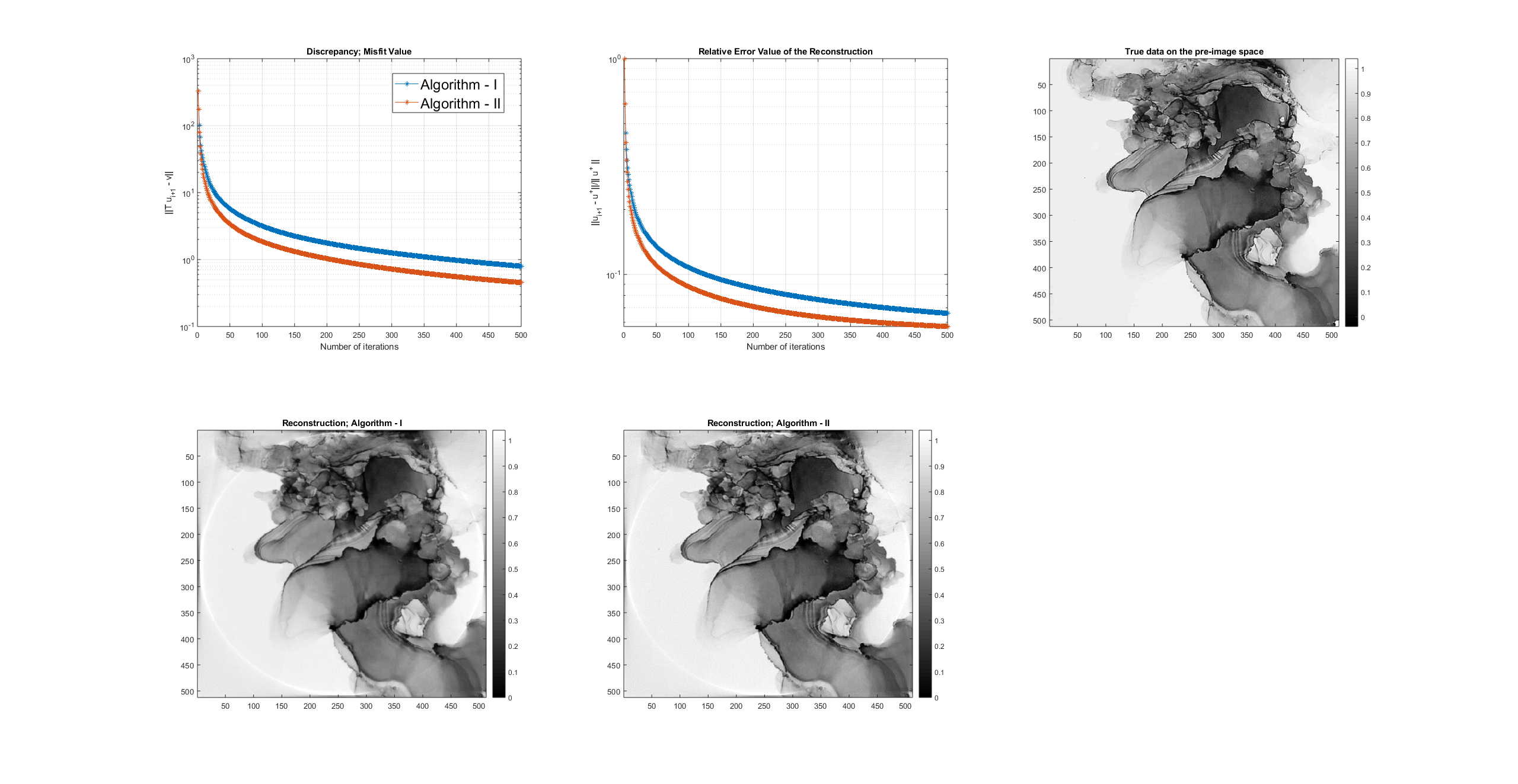
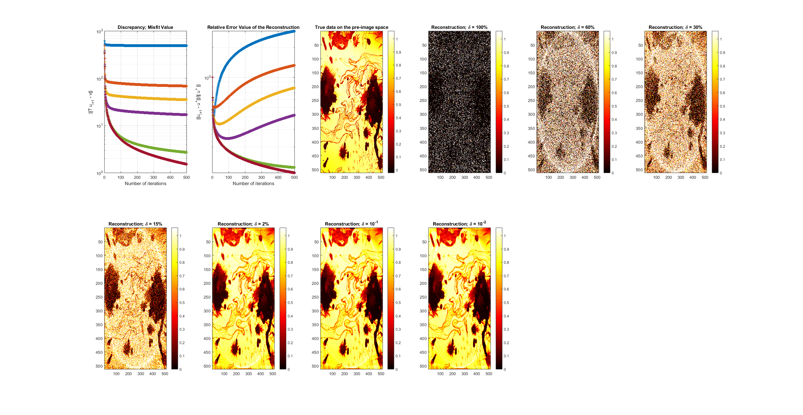
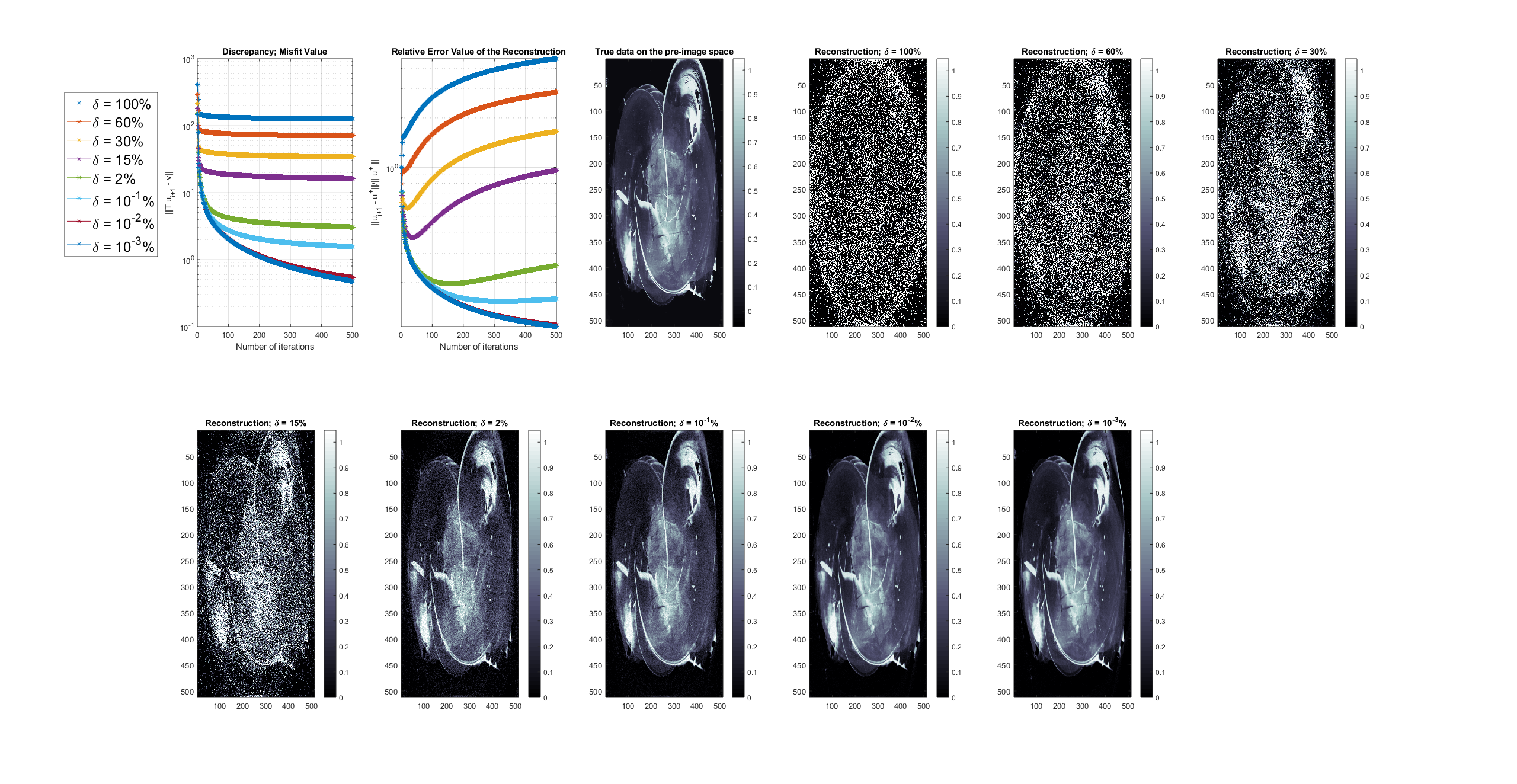
As can be seen in the Figures 2 and 3, it is verified that the less noise amount in the measured data provide less error estimation both on the image and the pre-image spaces.

Figure 2: Above results display the behaviour of the Algorithm 1 with the inclusion of different amount of noise on the measured data. Decay on the error estimations both on the image and the pre-image spaces has been observed with lesst noise amount.

Figure 3: Above results display the behaviour of the Algorithm 2 with the inclusion of different amount of noise on the measured data. Decay on the error estimations both on the image and pre-image spaces has been observed with lesst noise amount.

7 An Atmospheric Tomography Problem: GPS Tomography

One important predictor in meteorology is the humidity of the atmosphere. This is estimated by fan-beam measurements between satellite transmitters and land-based receivers. The measurements are sparse and fluctuate randomly with receiver availability. The task is to reconstruct from these measurements the 3-dimensional, spatially varying index of refraction of the atmosphere, from which the relative humidity can be inferred.

GPS-tomography involves the reconstruction of some quantity (e.g. humidity), pointwise within a volume, from geodesic X-ray measurements transmitted by nonuniformly distributed transducers (satellites). These measurements are collected by nonuniformly distributed receivers on the ground (ground stations). As in the conventional tomography, the task here is the reconstruction of the density volume profile of a layer in the atmosphere from a set of line integrals that are of fan-beam projections.

Function reconstruction from its measured line integrals was firstly proposed and solved in [66]. Profound mathematical and numerical aspects of the computerized tomography have been studied in [59, 61]. Measurement from the Radon transform is obtained by integrating some integrable function over the hyperplanes in $\mathbb{R}^{N}.$ The ray transform, on the other hand, produces measurement by integrating the function over straight lines. It is known that in the two dimensional tomography, general Radon and ray transformations coincide, [61, p. 17].

In the discretized form of the problem, it is assumed that each station receives equal number of signals transmitted by the satellites. Also for the sake of simplicity, we ignore any deviations from the shortest path between transmitters and receivers due to atmospheric refractivity. The received signal is then modelled as a line integral along the shortest path between the satellites and the ground stations.

Peculiar to this problem, reconstructions by Kalman filtering and ART have been widely applied, [13, 57, 65, 84]. Different from these conventional numerical reconstruction methods, a quasi-Newton approach, which is limited memory BFGS (L-BFGS), has also been proposed to obtain the optimal regularized solution, [2]. The L-BFGS algorithm has been also applied for atmospheric imaging wherby the forward problem has been modelled as a phase retrieval problem, see [78].

7.1 Physical Problem

This is an inverse problem with incomplete data. It is well known that the incompleteness of data causes nonuniqueness issue in inverse problems, [61, p. 144]. Thorough implementation and inversion of geodesic X-ray transform has been studied in [58]. The model of this problem is also widely known. We refer readers to [2] how the compact support assumption on the targeted data has been established for satisfying unique solvibility of the problem.

7.2 Numerical Results; Response of the algorithms to GPS-Tomography

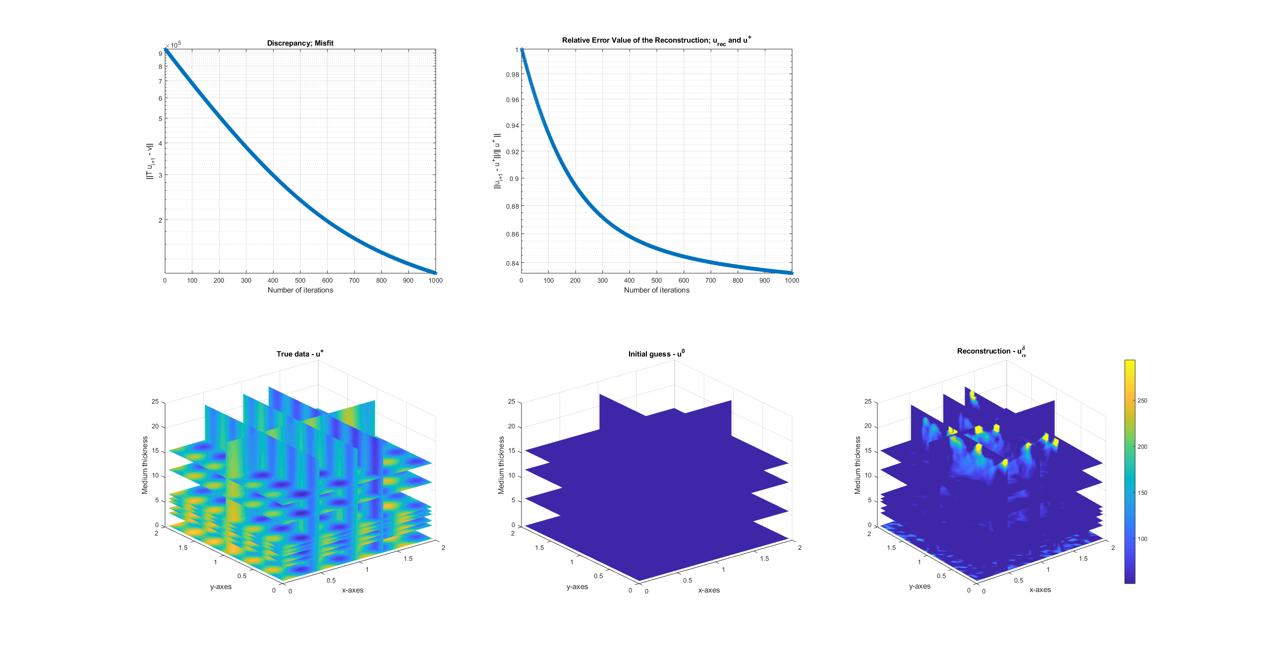
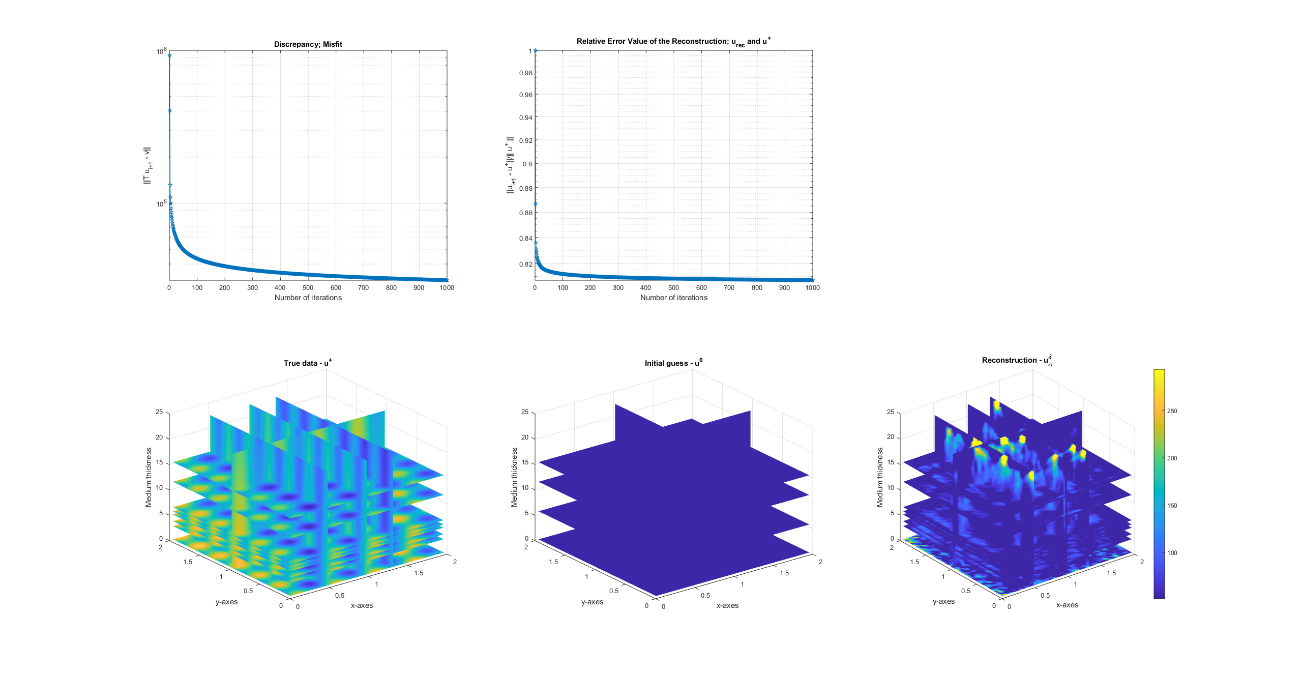
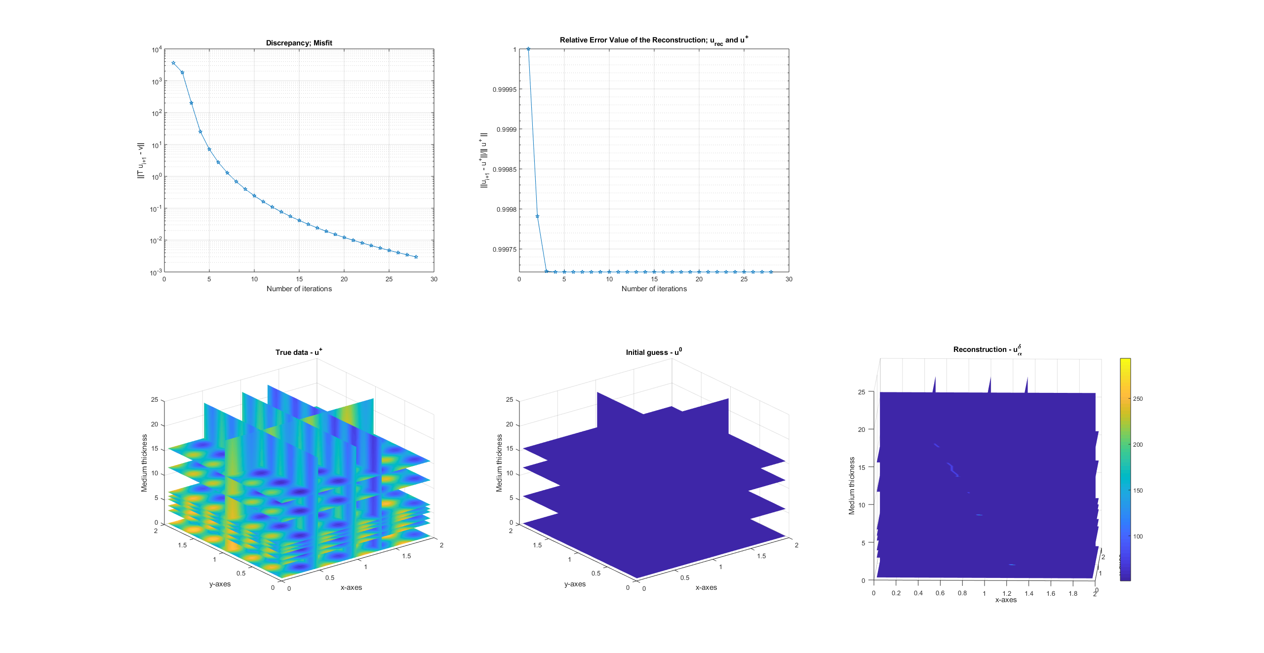
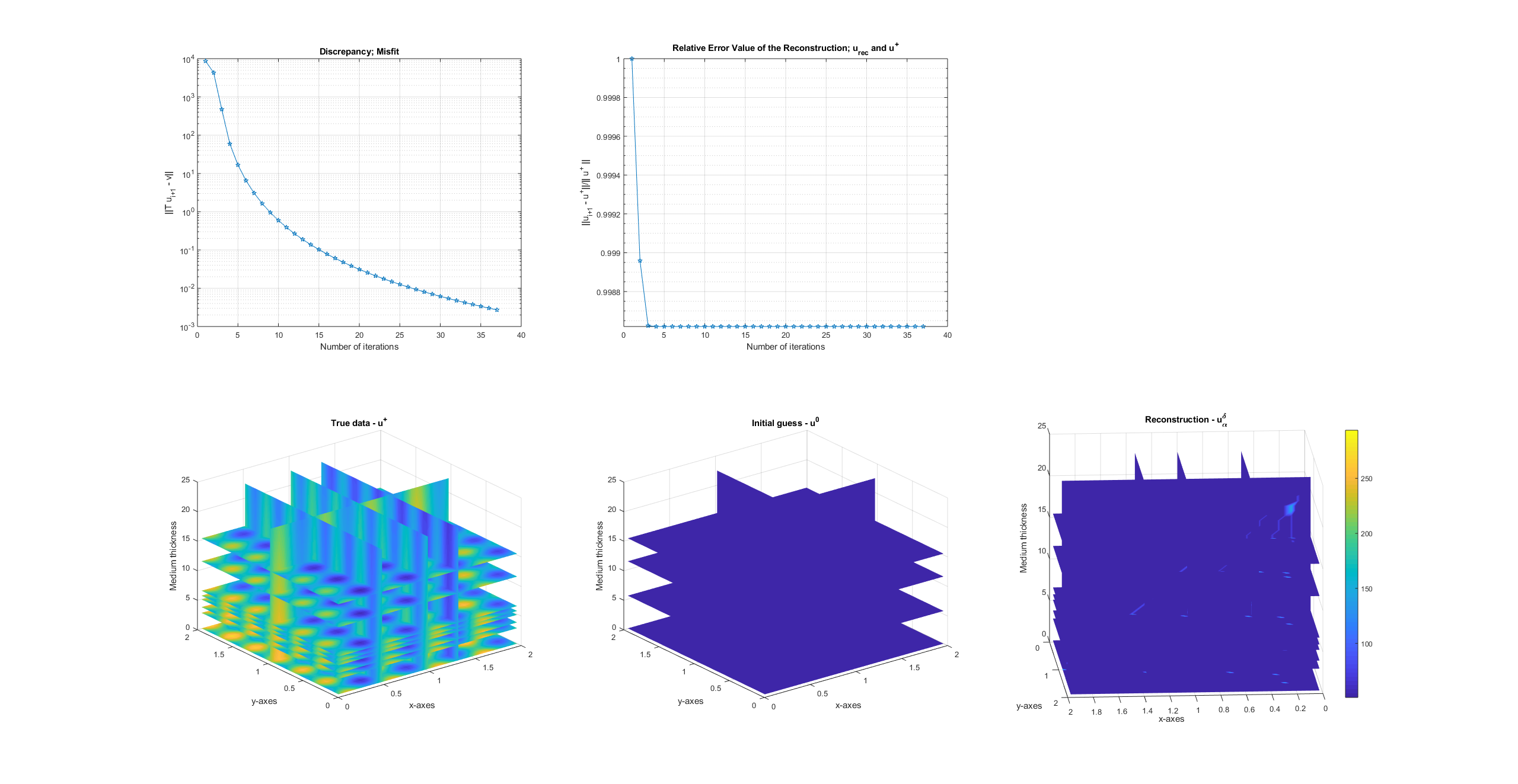
Above section has already been dedicated to understand that the algorithms are iterative regularization procedures, furthermore it has been demonstrated that Algorithm 2 provide better results. Thus in this section, we will rather present the numerical results of Algorithm 2 when it is applied to the GPS-Tomography problem. Specifically in this problem, recent novel reserch works [81, 83] indicate the importance of the number and the sources of the measured data. In this work, we are only able to emphasize that how number of the measurement data, e.g. the signals, affects the quality of the reconstructed data. In Figure 4, the numerical results have been produced when all the parameters are chosen as fixed coefficient. Figure 4 display the results when the parameters are dynamically chosen. Having a comparison two results against each other, dynamical choice of the parameters allow us to obtain better results with much less iteration steps during the procedure. Regarding the impact of the number of the measured data on the reconstruction, Figures 6 and 7 display less quality on the reconstructed data when the problem is defined as underdetermined.

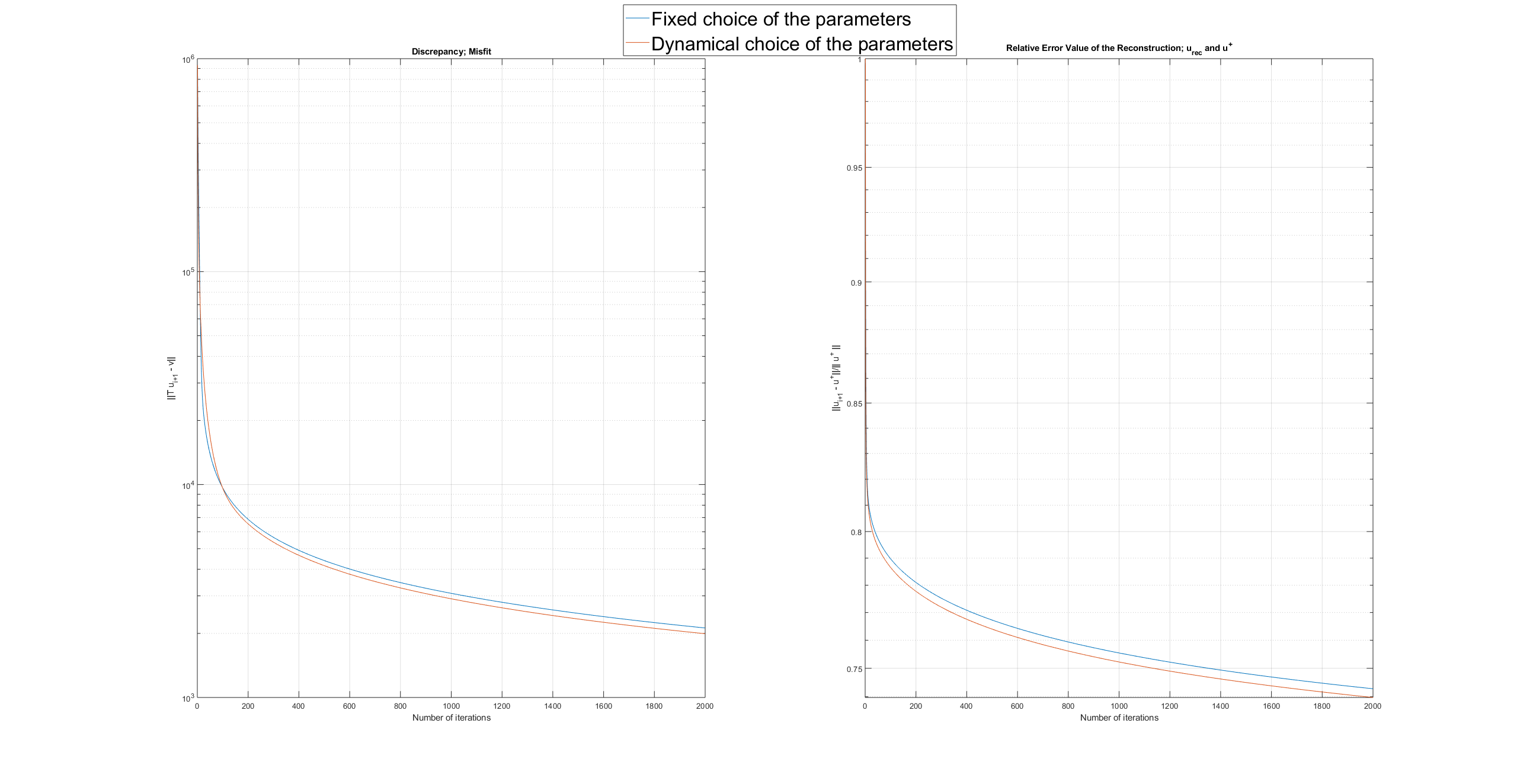
In the Figure 8, we demonstrate the importance of the parameter choices. As in the numerical results, with the dynamically chosen parameters, one can observe less error estimation at the end of the procedures.

Figure 4: Reconstruction of the volume data when all the parameters are chosen as fixed coefficients.

Figure 5: Reconstruction of the volume data when all the parameters are chosen dynamically.

Figure 6: Reconstruction of the volume data from single ray. In the reconstructed data, the trace of the signal can be seen.

Figure 7: Reconstruction of the volume data from five rays.

Figure 8: Benchmark on dynamical and static parameter choices. Numerical results are from Algorithm 2 applied to the GPS-Tomography problem.

8 Discussion and Future Prospects

Having the initial guess as constant in the mathematical analysis may not reveal the purpose of having Bregman distance as penalizer in our objective functional (2.7). Therefore, it could be worthwhile to consider the following iteration scheme

$$u_{i+1}\in{\rm arg\,min}_{u\in{\mathcal{X}}}\frac{1}{2}||Tu-v^{\delta}||^{2}+\alpha_{k}D_{J}(u,u_{k})+h(u).$$

Then, as a result of some quick calculations, the subdifferential characterization of the iterative minimizer is given by

$$\left\{\begin{array}[]{rcl}u_{i+1}&=&\mathrm{prox}_{\mu_{i}h}\left[u_{i+1}-\mu_{i}\left(T^{T}(Tu_{i+1}-v^{\delta})+\alpha_{i}D^{T}(w_{i+1}-w_{i})\right)\right]\\ w_{i+1}&=&\mathrm{prox}_{\nu_{i}g^{\ast}}\left(w_{i+1}+\nu_{i}Du_{i+1}\right).\end{array}\right.$$ (8.3)

An algorithm solving this system will definitely convey minimization impact when the iterative form of Bregman distance is introduced as penalty term.

References

- [1] R. Acar, C. R. Vogel. Analysis of bounded variation penalty methods for ill-posed problems, Inverse Problems, Vol. 10, No. 6, 1217 - 1229, 1994.
- [2] E. Altuntac. Variational Regularization Strategy for Atmospheric Tomography. Institute for Numerical and Applied Mathematics, University of Goettingen, July 2016.
- [3] E. Altuntac. Choice of the Parameters in A Primal-Dual Algorithm for Bregman Iterated Variational Regularization. https://arxiv.org/abs/1807.05793, 2018.
- [4] L. Ambrosio, N. Fusco, and D. Pallara. Functions of bounded variation and free discontinuity problems. Oxford Mathematical Monographs. The Clarendon Press, Oxford University Press, New York, 2000.
- [5] S. Anzengruber, B. Hofmann and P. Mathé. Regularization properties of the sequential discrepancy principle for Tikhonov regularization in Banach spaces. Appl. Anal. 93, 7, 1382 -1400, 2014.
- [6] S. Anzengruber and R. Ramlau. Morozov’s discrepancy principle for Tikhonov-type functionals with nonlinear operators. Inverse Problems, 26, 025001 (17pp), 2010.
- [7] S. Anzengruber and R. Ramlau. Convergence rates for Morozov’s discrepancy principle using variational inequalities. Inverse Problems, 27, 105007 (18pp), 2011.
- [8] M. Bachmayr and M. Burger. Iterative total variation schemes for nonlinear inverse problems, Inverse Problems, 25, 105004 (26pp), 2009.
- [9] J. Bardsley. MATLAB codes for “Computational Uncertainty Quantification for Inverse Problems,“ 2018. https://github.com/bardsleyj/SIAMBookCodes.
- [10] H. H. Bauschke, P. L. Combettes. Convex analysis and monotone operator theory in Hilbert spaces, Springer New York, 2011.
- [11] J. M. Bardsley and A. Luttman. Total variation-penalized Poisson liklehood estimation for ill-posed problems, Adv. Comput. Math., 31:25-59, 2009.
- [12] A.Beck and M.Teboulle. A Fast Iterative Shrinkage-Thresholding Algorithm for Linear Inverse Problems. SIAM J. Imaging Sciences, Vol. 2, No. 1, pp. 183-202, 2009.
- [13] M. Bender, G. Dick, M. Ge, Z. Deng, J. Wickert, H. G. Kahle, A. Raabe, G. Tetzlaff. Development of a GNSS water vapour tomography system using algebraic reconstruction technique, ADV SPACE RES, 47(10):1704-1720, 2011.
- [14] M. Benning and M. Burger. Modern Regularization Methods for Inverse Problems. https://arxiv.org/pdf/1801.09922, 2017.
- [15] M. Benning, M. M. Betcke, M. J. Ehrhardt, C.-B. Schönlieb. Choose your path wisely: gradient descent in a Bregman distance framework, arXiv:1712.04045, 2017.
- [16] M. Bergounioux. On Poincaré-Wirtinger inequalities in space of functions bounded variation. Control Cybernet., 40, 4, 921-29, 2011.
- [17] T. Bonesky, K. S. Kazimierski, P. Maass, F. Schöpfer, T. Schuster. Minimization of Tikhonov Functionals in Banach Spaces, Abstr. Appl. Anal., Art. ID 192679, 19 pp, 2008.
- [18] S. Bonettini, I. Loris, F. Porta, M. Prato and S. Rebegoldi. On the convergence of a linesearch based proimal-gradient method for nonconvex optimization. Inverse Problems, 33, 055005 (30pp), 2017.
- [19] J. Borwein and R. Luke. Entropic Regularization of the Function. In: Bauschke H., Burachik R., Combettes P., Elser V., Luke D., Wolkowicz H. (eds) Fixed-Point Algorithms for Inverse Problems in Science and Engineering. Springer Optimization and Its Applications, vol 49. Springer, New York, NY, 2011.
- [20] K. Bredies. A forward-backward splitting algorithm for the minimization of non-smooth convex functionals in Banach space, Inverse Problems 25, no. 1, 015005, 20 pp, 2009.
- [21] M. Burger, S. Osher. Convergence rates of convex variational regularization, Inverse Problems, 20(5), 1411 - 1421, 2004.
- [22] A. Chambolle. An algorithm for Total Variation Minimization and Applications. J. Math. Imaging Vis., 20, 89 - 97, 2004.
- [23] A. Chambolle, Vicent Caselles, Matteo Novaga, Daniel Cremers, Thomas Pock. An introduction to Total Variation for Image Analysis. hal-00437581, 2009.
- [24] A. Chambolle, P. L. Lions. Image recovery via total variation minimization and related problems, Numer. Math. 76, 167 - 188, 1997.
- [25] T. F. Chan and K. Chen. An optimization-based multilevel algorithm for total variation image denoising, Multiscale Model. Simul. 5, no. 2, 615-645, 2006.
- [26] T. Chan, G. Golub and P. Mulet. A nonlinear primal-dual method for total variation-baes image restoration, SIAM J. Sci. Comp 20: 1964-1977, 1999.
- [27] J. Chen and I. Loris On starting and stopping criteria for nested primal-dual iterations. arXiv:1806.07677, 2018.
- [28] F. H. Clarke. Optimization and Nonsmooth Analysis. Classics in Applied Mathematics, 5, SIAM, 1990.
- [29] D. Colton and R. Kress. Inverse Acoustic and Electromagnetic Scattering Theory, Springer Verlag Series in Applied Mathematics Vol. 93, Third Edition 2013.
- [30] P.L. Combettes and JC. Pesquet. Proximal Splitting Methods in Signal Processing. In: Bauschke H., Burachik R., Combettes P., Elser V., Luke D., Wolkowicz H. (eds) Fixed-Point Algorithms for Inverse Problems in Science and Engineering. Springer Optimization and Its Applications, vol 49. Springer, New York, NY, 2011.
- [31] M. Defrise, C. Vanhove, and X. Liu. An algorithm for total variation regularization in high-dimensional linear problems, Inverse Problems 27 065002 (16pp), 2011.
- [32] D. Dobson, O. Scherzer. Analysis of regularized total variation penalty methods for denoising, Inverse Problems, Vol. 12, No. 5, 601 - 617, 1996.
- [33] D. C. Dobson, C. R. Vogel. Convergence of an iterative method for total variation denoising, SIAM J. Numer. Anal., Vol. 34, No. 5, 1779 - 1791, 1997.
- [34] H. W. Engl, M. Hanke, A. Neubauer. Regularization of inverse problems, Math. Appl., 375. Kluwer Academic Publishers Group, Dordrecht, 1996.
- [35] J. Flemming. Existence of variational source conditions for nonlinear inverse problems in Banach spaces. J. Inverse Ill-Posed Probl., 26, 2, 277 - 286, 2018.
- [36] J. M. Fowkes, N. I. M. Gould, C. L. Farmer. A branch and bound algorithm for the global optimization of Hessian Lipschitz continuous functions, J. Glob. Optim., 56, 1792 - 1815, 2013.
- [37] G. Garrigos, L. Rosasco and S. Villa. Iterative regularization via dual diagonal descent. J Math Imaging Vis, 60, 2, 189 - 215, 2018.
- [38] M. Grasmair. Generalized Bregman distances and convergence rates for non-convex regularization methods, Inverse Problems 26, 11, 115014, 16pp, 2010.
- [39] M. Grasmair. Variational inequalities and higher order convergence rates for Tikhonov regularisation on Banach spaces, J. Inverse Ill-Posed Probl., 21, 379-394, 2013.
- [40] M. Grasmair, M. Haltmeier, O. Scherzer. Necessary and sufficient conditions for linear convergence of -regularization, Comm. Pure Appl. Math. 64(2), 161-182, 2011.
- [41] C. W. Grötsch. Inverse problems in the mathematical sciences, Vieweg, 1993.
- [42] C. W. Grötsch. Integral equations of the first kind, inverse problems and regularization: a crash course, J. Phys.: Conf. Ser. 73 012001, 2007.
- [43] P. C. Hansen. Rank deficient and discrete ill-posed problems: Numerical aspects of linear inversion, SIAM Monogr. Math. Model. Comput., Philadelphia, 1998.
- [44] C. Hamaker, K. T. Smith, D. C. Solmon, S. L. Wagner. The divergent beam x-ray transform, Rocky Mountain J. Math., 10, No.1, 253 - 283, 1980.
- [45] B Hofmann, B. Kaltenbacher, C. Pöschl and O. Scherzer. A convergence rates results for Tikhonov regularization in Banach spaces with non-smooth operator. Inverse Problems, 23(3), 987 - 1010, 2007.
- [46] B. Hofmann and P. Mathé. Parameter choice in Banach space regularization under variational inequalities. Inverse Problems 28, 104006 (17pp), 2012.
- [47] B. Hofmann, B. Kaltenbacher, C. P‘̀oschl, and O. Scherzer. A convergence rates result for Tikhonov regularization in Banach spaces with non-smooth operator. Inverse Problems, 23 (3), 987 - 1010, 2007.
- [48] T. Hohage and F. Weidling. Verification of a variational source condition for acoustic inverse medium scattering problems. Inverse Problems, 31, 075006 (14pp), 2015.
- [49] T. Hohage and C. Schormann. A Newton-type method for a transmission problem in inverse scattering. Inverse Problems 14, 1207 - 1227, 1998.
- [50] T. Hohage and F. Weidling. Characterizations of variational source conditions, converse results, and maxisets of spectral regularization methods. arXiv:1603.05133, 2016.
- [51] V. Isakov. Inverse problems for partial differential equations. Second edition. Applied Mathematical Sciences, 127. Springer, New York, 2006.
- [52] S. Kindermann. Convex Tikhonov regularization in Banach spaces: New results on convergence rates. J. Inverse Ill-Posed Probl., 24, 3, 341 - 350, 2016.
- [53] A. Kirsch. An introduction to the mathematical theory of inverse problems. Second edition. Applied Mathematical Sciences, 120. Springer, New York, 2011.
- [54] D. A. Lorenz. Convergence rates and source conditions for Tikhonov regularization with sparsity constraints, J. Inv. Ill-Posed Problems, 16, 463-478, 2008.
- [55] I. Loris and C. Verhoeven. On a generalization of the iterative soft-thresholding algorithm for the case of non-separable penalty. Inverse Problems, 27, 125007, 15pp, 2011.
- [56] C. Louchet and L. Moisan. Total Variation as a Local Filter. SIAM J. I MAGING S CIENCES, Vol. 4, No. 2, pp. 651 - 694, 2011.
- [57] P. Miidla, K. Rannat P. Uba. Tomographic approach for tropospheric water vapor detection, Comput. Methods. Appl. Math., 8(3), 263-278, 2008.
- [58] F. Monard. Numerical Implementation of Geodesic X-Ray Transforms and Their Inversion. SIAM J. IMAGING SCIENCES, 7, 2, 1335 - 1357, 2014.
- [59] F. Natterer. The mathematics of computerized tomography, SIAM, Classics Appl. Math., 32, 2001.
- [60] F. Natterer. X-ray Tomography. Inverse Problems and Imaging, Springer, Berlin, 17 - 34, 2008.
- [61] F. Natterer and F. Wübbeling. Mathematical methods in image reconstruction, SIAM Monogr. Math. Model. Comput., 05, 2001.
- [62] G. Ólafsson, E. T. Quinto. The Radon transform, inverse problems and tomography, Proceedings of Symposia in Applied Mathematics, Volume 63, American Mathematical Society Short Course, January 3-4, 2005, Atlanta, Georgia, 2006.
- [63] S. S. Orlov. Theory of three dimensional reconstruction II: The recovery operator. Soviet Phys. Crystallogr., 20, 429 - 433, 1976.
- [64] S. Osher, M. Burger, D. Goldfarb, J. Xu and W. Yin. An Iiterative Regularization Method for Total Variation-Based Image Restoration. Multiscale Model. Simul., 4(2), 460 - 489, 2005.
- [65] D. Perler, A. Geiger and F. Hurter. 4D GPS water vapor tomography: new parameterized approaches. J. Geod., 85, 539-550, 2011.
- [66] J. Radon. Über die Bestimmung von Funktionnen durch ihre Integralwerte längs gewisser Mannigfaltikeiten, Ber. Verh. Sachs. Akad. Wiss. Leipzig-Math.-Natur. Kl., 69, 262 - 277, 1917.
- [67] R.T. Rockafellar, R. J.-B. Wets. Variational Analysis. Fundamental Principles of Mathematical Sciences, 317. Springer-Verlag, Berlin, 1998.
- [68] L. I. Rudin, S. J. Osher, E. Fatemi. Nonlinear total variation based noise removal algorithms, Physica D, 60, 259-268, 1992.
- [69] O. Scherzer, M. Grasmair, H. Grossauer, M. Haltmeier and F. Lenzen. Variational Methods in Imaging. Applied Mathematical Sciences, 167, Springer, New York, 2009.
- [70] U. Schröder and T. Schuster. An Iterative Method to Reconstruct the Refractive Index of a Medium From Time-of-Flight Measurements. arXiv:1510.06899v1 , 2015.
- [71] T. Schuster, B. Kaltenbacher, B. Hofmann, K.S. Kazimierski. Regularization Methods in Banach Spaces. RICAM, 10, De Gruyter, 2012.
- [72] D. F. Shanno and K. Phua. Matrix conditioning and nonlinear optimization. Math. Prog., 14, 149 - 160, 1978.
- [73] K. T. Smith, D. C. Solmon, S. L. Wagner, C. Hamaker. Mathematical aspects of divergent beam radiography, Proc. Natl. Acad. Sci. USA, 75, No. 5, 2055 - 2058, 1978.
- [74] B. Sprung and T. Hohage. Higher order convergence rates for Bregman iterated variational regularization of inverse problems. arXiv:1710.09244, 2017.
- [75] W. Takahashi, N.C. Wong and J.C. Yao. Fixed point theorems for nonlinear non-self mappings in Hilbert spaces and applications. JFPTA, 2013:116, 2013.
- [76] A. N. Tikhonov. On the solution of ill-posed problems and the method of regularization, Dokl. Akad. Nauk SSSR, 151, 501-504, 1963.
- [77] A. N. Tikhonov, V. Y. Arsenin. Solutions of ill-posed problems. Translated from the Russian. Preface by translation editor Fritz John. Scripta Series in Mathematics. V. H. Winston & Sons, Washington, D.C.: John Wiley & Sons, New York-Toronto, Ont.-London, xiii+258 pp, 1977.
- [78] C. R. Vogel. A limited memory BFGS method for an inverse problem in atmospheric imaging. Methods and Applications of Inversion, Lecture Notes in Earth Sciences, 92, 292-304, 2000.
- [79] C. R. Vogel. Computational methods for inverse problems, Frontiers Appl. Math. 23, 2002.
- [80] C. R. Vogel , M. E. Oman. Iterative methods for total variation denoising, SIAM J. SCI. COMPUT., Vol. 17, No. 1, 227-238, 1996.
- [81] Z. Xiong, B. Zhang and Y. Yao. Comparisons between the WRF data assimilation and the GNSS tomography technique in retrieving -D wet refractivity fields in Hong Kong. Ann. Geophys., 37, 25-36, 2019.
- [82] W. Yin, S. Osher, D. Goldfarb and J. Darbon. Bregman Iterative Algorithms for Minimization with Applications to Compressed Sensing. SIAM J. Imaging Sciences, Vol. 1, N0. 1, pp.143 - 168, 2008.
- [83] Q. Zhao, Y. Yao, X. Cao and W. Yao. Accuracy and reliability of tropospheric wet refractivity tomography with GPS, BDS, and GLONASS observations. Adv. Space Res. (2018), https://doi.org/10.1016/j.asr.2018.01.021
- [84] F. Zus, M. Bender, Z. Deng, G. Dick, S. Heise, M. Shang-Guan, J. Wickert, A methodology to compute GPS slant total delays in a numerical weather model, Radio Science, 2012, vol. 47, RS2018.