HST/STIS analysis of the first main sequence pulsar CU Vir

Abstract

Context. CU Vir has been the first main sequence star that showed regular radio pulses that persist for decades, resembling the radio lighthouse of pulsars and interpreted as auroral radio emission similar to that found in planets. The star belongs to a rare group of magnetic chemically peculiar stars with variable rotational period.

Aims. We study the ultraviolet (UV) spectrum of CU Vir obtained using STIS spectrograph onboard the Hubble Space Telescope (HST) to search for the source of radio emission and to test the model of the rotational period evolution.

Methods. We used our own far-UV and visual photometric observations supplemented with the archival data to improve the parameters of the quasisinusoidal long-term variations of the rotational period. We predict the flux variations of CU Vir from surface abundance maps and compare these variations with UV flux distribution. We searched for wind, auroral, and interstellar lines in the spectra.

Results. The UV and visual light curves display the same long-term period variations supporting their common origin. New updated abundance maps provide better agreement with the observed flux distribution. The upper limit of the wind mass-loss rate is about $10^{-12}\,M_{\odot}\,\text{yr}^{-1}$. We do not find any auroral lines. We find rotationally modulated variability of interstellar lines, which is most likely of instrumental origin.

Conclusions. Our analysis supports the flux redistribution from far-UV to near-UV and visual domains originating in surface abundance spots as the main cause of the flux variability in chemically peculiar stars. Therefore, UV and optical variations are related and the structures leading to these variations are rigidly confined to the stellar surface. The radio emission of CU Vir is most likely powered by a very weak presumably purely metallic wind, which leaves no imprint in spectra.

1 Introduction

The magnetic chemically peculiar star CU Virginis (HR 5313, HD 124224) is one of the most enigmatic stars of the upper part of the main sequence. CU Vir shows continuum radio emission, explained as due to gyrosynchrotron process from electrons spiraling in a co-rotating magnetosphere. According to Leto et al. (2006), a stellar wind with mass-loss rate on the order of $10^{-12}\,{M}_{\odot}\,\text{yr}^{-1}$ is a source of free electrons. But the most intriguing behavior of CU Vir is the presence of a coherent, highly directive radio emission at 1.4 GHz, at particular rotational phases, interpreted as electron cyclotron maser emission (Trigilio et al. 2000; Ravi et al. 2010; Lo et al. 2012). In this interpretation, CU Vir is similar to a pulsar, even if the emission process is different, resembling auroral activity in Earth and major planets (Trigilio et al. 2011). This type of emission is not unique among hot stars, as evidenced by the detection of electron cyclotron maser emission from other magnetic chemically peculiar stars (Das et al. 2018; Lenc et al. 2018; Leto et al. 2019). The auroral radio emission from stars with a dipole-like magnetic field has been modeled by Leto et al. (2016). This opens a new theoretical approach to the study of the stellar auroral radio emission and, in particular, this method could be used to identify the possible signature of a star-planet magnetic interaction (like the Io-Jupiter interaction, Hess & Zarka 2011; Leto et al. 2017).

However, a star with parameters that correspond to CU Vir is not expected to have a stellar wind required to explain the observed continuum radio emission (Krtička 2014). Moreover, weak winds are subject to decoupling of metals (Owocki & Puls 2002; Krtička & Kubát 2002; Votruba et al. 2007), which has not yet been observationally verified. Consequently, the detection of “auroral” utraviolet (UV) lines is desirable to further support to the current model of pulsed radio emission.

CU Vir belongs to the group of hot magnetic chemically peculiar stars. These hot stars are usually slowly rotating, and possess notable outer envelopes mostly without convective and meridional motions. This allows the radiatively driven diffusion to be effective, and with occurrence of a global (possibly fossil) magnetic field, it may give rise to the chemical peculiarity and consequently to persistent surface structures (Michaud 2004; Alecian et al. 2011). These structures manifest themselves in a periodic spectrum and spectral energy distribution variability, frequently accompanied by variations of the effective magnetic field (Kuschnig et al. 1999; Lüftinger et al. 2010; Kochukhov et al. 2014). The persistent surface structures (spots) differ from transient dark solar-type spots that originate due to the suppression of convective motion in the regions with enhanced local magnetic field and last for short time scales only.

The detailed nature of the rotationally modulated light variability of chemically peculiar stars remained elusive for decades. The problem became clearer after application of advanced stellar model atmospheres calculated assuming elemental surface distributions derived from surface Doppler mapping based on optical spectroscopy. This enabled us to construct photometric surface maps and to predict light variability (e.g., Krtička et al. 2012; Prvák et al. 2015). The result supports the current paradigm for the nature of the light variability of chemically peculiar stars, according to which this light variability is caused by the redistribution of the flux from the far-UV to near-UV and visible regions due to the bound-bound (lines, mainly iron or chromium, Kodaira 1973; Molnar 1973) and bound-free (ionization, mainly silicon and helium, Peterson 1970; Lanz et al. 1996) transitions, the inhomogeneous surface distribution of elements, and modulated by the stellar rotation. However, in CU Vir this model is not able to explain fully the observed UV and optical light variability (Krtička et al. 2012), particularly in the Strömgren $u$ color and around $1600\,$Å in the UV domain.

Moreover, being an unusually fast rotator, CU Vir  belongs to a rare group of magnetic chemically peculiar stars that show secular variations of the rotation period (Pyper et al. 1998, 2013; Mikulášek et al. 2011; Mikulášek 2016). These variations were interpreted as a result of torsional oscillations (Krtička et al. 2017), which stem from the interaction of an internal magnetic field and differential rotation (Mestel & Weiss 1987). The variations were not, however, directly detected in the UV domain.

All these open problems connected with the atmosphere, magnetosphere, and wind of CU Vir can be adequately addressed by dedicated high-resolution UV observations. Here we describe our HST/STIS observations aiming to get a more detailed picture of the CU Vir UV light variability and its magnetosphere.

2 Observations

2.1 HST and IUE ultraviolet observations

Our HST observations were collected within the program #14737 using the STIS spectrograph with 31X0.05NDA slit, E140H grating in positions corresponding to the central wavelengths 1380 Å and 1598 Å, and using the FUV-MAMA detector. The observations are homogeneously distributed over CU Vir rotational phase and cover the wavelength regions 1280 – 1475 Å and 1494 – 1688 Å (see Table 1). The observations were processed via standard STIS pipelines and were downloaded from the MAST archive. We further applied the median filter to reduce the noise in the spectra.

Table 1: HST/STIS observations of CU Vir.

Spectrum	Region [Å]	HJDmean	mean phase
od5y02010	1380	2 457 948.6933	0.220
od5y02020	1598	2 457 948.7062	0.245
od5y03010	1380	2 457 945.6472	0.370
od5y03020	1598	2 457 945.6602	0.395
od5y04010	1380	2 457 953.5934	0.631
od5y04020	1598	2 457 953.6067	0.657
od5y05010	1380	2 457 947.4351	0.804
od5y05020	1598	2 457 947.4480	0.828
od5y51010	1380	2 458 254.2392	0.036
od5y51020	1598	2 458 254.2522	0.061

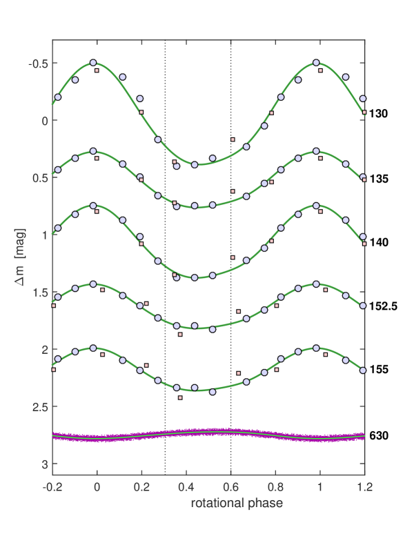
Figure 1: Comparison of light curves in far UV and red regions of CU Vir spectrum. Blue circles and red squares denote synthetic magnitudes derived from IUE and STIS spectra and lilac points are the measurements from SMEI satellite. Wavelengths are expressed in nanometers. Phases are calculated using ephemeris Eq. (4) applying parameters given in Table 2. Green lines are the fits of the light curve phenomenological model Eq. (3.1), assuming two photometric spots with photocenters at the phases 0.303 and 0.598 (denoted using vertical black dotted lines). Light curves were plotted relative to the mean value of the fits and vertically shifted to separate individual plots.

Observations from the HST nicely cover the rotation cycle of the star (see Fig. 1). The observations close to the phase $\varphi\approx 0$ correspond to visual minimum and to UV maximum. This is also the phase of the start of XMM-Newton X-ray observation ($\varphi\approx 0.07$, Robrade et al. 2018). The spectra od5y02010 and od5y02020 correspond to the period of X-ray quiescence roughly 7 ks after the start of observation. The spectrum od5y03010 was obtained close to the $a$ peak of radio emission, which is observed around the phases $0.29-0.35$ (Trigilio et al. 2008). This is also approximately the period of maximum strength of Si lines, which appears roughly around the phase $\varphi\approx 0.35$ (Kuschnig et al. 1999) and which corresponds to strong X-ray flux roughly 15 ks after the start of XMM-Newton observations. The maximum strength of Fe lines and optical maximum is observed slightly later around the phase $0.5$. The spectrum od5y04020 marks the end of XMM-Newton observations. The peak $b$ of radio emission is located around $\varphi=0.71-0.77$, close to which the spectrum od5y05010 was obtained. This also roughly marks the start of Chandra observations ($\varphi=0.76$). These observations end at $\varphi=0.40$.

We supplemented the HST CU Vir observations with IUE data (PI: M. Maitzen, see Sokolov 2000; Krtička et al. 2012, hereafter Paper I). To obtain the UV photometry, we extracted IUE observations of CU Vir from the INES database using the SPLAT package (Draper 2004, see also Škoda 2008). We downloaded low-dispersion data originating from high-dispersion large aperture spectra in the domains 1250–1900 Å (SWP camera) and 2000–3000 Å (LWR camera). For the spectroscopic analysis, we used high-dispersion IUE data downloaded from the MAST archive. We compared the absolute flux normalization of HST and IUE spectra concluding that these flux normalizations are consistent (within small differences which can be attributed to calibration).

We used the HST and IUE SWP fluxes $F(\lambda)$ to calculate UV magnitudes (see Fig. 1)

$$m_{c}=-2.5\log\left[\int_{0}^{\infty}\mathit{\Phi}_{c}(\lambda)F(\lambda)\,\text{d}\lambda\right],$$ (1)

where $\mathit{\Phi}_{c}(\lambda)=\left(\sqrt{\pi}\sigma\right)^{-1}\exp\left(-{(\lambda-c)^{2}}/{\sigma^{2}}\right)$ is a normalized Gauss function centered on the wavelength $c$. The central wavelengths of individual Gauss filters cover HST spectra, $c=1300\,\AA$, $1350\,\AA$, $1400\,\AA$, $1525\,\AA$, and $1550\,\AA$. The dispersion was selected $\sigma=10\,\AA$ for $c=1300\,\AA$ and $1525\,\AA$, and $\sigma=25\,\AA$ for the remaining ones. Figure 1 shows that the IUE and HST light curves are very similar with small differences most likely due to instrumental calibration.

We derived the synthetic photometry from IUE LWR spectra also using Eq. (1) (see Mikulášek et al. 2011). The UV synthetic photometry of HST and IUE was further supplemented by the data derived from OAO II satellite (Molnar & Wu 1978).

2.2 Standard photometry

In addition to the 326 photometric measurements derived from the UV spectra taken by HST and IUE and adopted from Molnar & Wu (1978), we also used 35 803 other available photometric data obtained in the time interval 1972 – 2018 by various observers in the region 330–753 nm using standard photometric techniques (see Mikulášek 2016, for the list). We supplemented these data with two additional sets of observations.

From 2010 February through 2018 June, we acquired 1191 photometric observations in the Johnson $V$ band and 1327 in the Johnson $B$ band, with Tennessee State University’s T3 0.40 m automatic photoelectric telescope (APT) at Fairborn Observatory in the Patagonia Mountains of southern Arizona (Henry 1999). Each observation in each filter represents the mean of three differential measurements of CU Vir bracketed by four measurements of its comparison star HD 125181. Details on the acquisition and reduction of the observations can be found in our paper on HR 7224 (Krtička et al. 2009).

The space photometry of CU Vir is available from the Solar Mass Ejection Imager (SMEI) experiment (Eyles et al. 2003; Jackson et al. 2004). The experiment was placed on-board the Coriolis spacecraft and aimed to measure sunlight scattered by free electrons of the solar wind. A by-product of the mission is the photometry of bright stars all over the sky, available through the University of California San Diego (UCSD) web page. The SMEI passband covers the range between 450 and 950 nm (Eyles et al. 2003). The photometry of stars was obtained using a technique developed by Hick et al. (2007). The SMEI stellar time series are affected by long-term calibration effects, especially a repeatable variability with a period of one year. They also retain unwanted signals from high energy particle hits and aurorae. Nevertheless, the SMEI observations are well suited for studying variability of bright stars primarily because they cover an extended interval – 2003 to 2010.

The raw SMEI UCSD photometry of CU Vir was first corrected for the one-year variability by subtracting an interpolated mean light curve. This curve was obtained by folding the raw data with the period of one year, calculating median values in 200 intervals in phase, and then interpolating between them. In addition, the worst parts of the light curve and outliers were removed. Then, a model consisting of the sinusoid with rotational frequency of CU Vir and its detectable harmonics was fitted to the data. The low-frequency instrumental variability was filtered out by subtracting trends that were calculated using residuals of the fit and removing outliers using $\sigma$-clipping. The trends were approximated by calculating averages in time intervals which were subsequently interpolated. The final SMEI light curve consists of 19 226 individual data points.

2.3 Optical spectroscopy

Additional optical spectra were obtained at Astronomical observatory in Piwnice (Poland). We used a mid-resolution echèlle spectrograph ($R\sim 15\,000$) connected via optical fiber to the 90 cm diameter Schmidt-Cassegrain telescope. Spectra were observed during two weekly runs in 2010 (March 3 – 10, April 4 – 8) and during one night in 2011 (February 10). Th-Ar calibration spectrum was taken before and after each scientific image. For reduction we used standard IRAF routines (bias, flat, and wavelength calibration). In total we collected 59 spectra, which cover wavelength regions from 4350 –7160 Å and all rotational phases of the star.

3 Long-term rotational period variations

The method used to monitor CU Vir long-term rotational period variations is based on the phenomenological modeling of phase function $\vartheta(t)$ (the sum of the phase and epoch) and periodic or quasiperiodic phase curves of tracers of the rotation (typically light curves), as the functions of $\vartheta(t)$. The phase function is connected with the generally variable rotational period $P(t)$ through the basic relations (see Mikulášek et al. 2008b; Mikulášek 2016):

$$\overset{\mathrm{\raisebox{-0.6458pt}{\hbox to0.0pt{\hss$\displaystyle\hskip 1.00006pt.$\hss}}}}{\vartheta}=\frac{1}{P(t)};\quad\vartheta(t)=\int_{M_{0}}^{t}\frac{\mathrm{d}\tau}{P(\tau)};\quad\theta(\vartheta)=\int_{0}^{\vartheta}P(\zeta)\,\mathrm{d}\zeta.$$ (2)

The phase function $\vartheta(t)$ is a smooth, monotonically rising function of time. The relation for its inversion function $\theta(\vartheta)$ can be derived from the same basic differential equation. Using the inversion phase function, we can predict, for example, times of maxima or other important moments of the phase variations.

3.1 Model of light curves

The light curves, obtained at various times in the filters of different effective wavelengths $\lambda_{\mathrm{eff}}$ from 130 to 753 nm, provide a massive amount of information about CU Vir rotation and its long-term variations. There is a general expectation (Paper I) that the shapes of CU Vir light curves strongly depend on the effective wavelengths (see Fig. 1). Nevertheless, the careful inspection revealed that all of the observed light curves can be satisfactorily expressed as a linear combination of only two symmetric basic profiles with centers at phases $\vartheta_{0j}$ and half-widths $d_{j}$:

$$\displaystyle F(\lambda_{\text{eff}},\vartheta)=\sum_{j=1}^{2}A_{j}(\lambda_{\text{eff}})\,\left\{\exp\left[1\!-\!\cosh\left(\frac{\Delta\varphi_{j}}{d_{j}}\right)\right]-2.29\,d_{j}\right\};$$

$$\mathrm{where}\quad\Delta\varphi_{j}=(\vartheta-\varphi_{0j})-\mathrm{round}(\vartheta-\varphi_{0j}),$$ (3)

where $F(\lambda_{\text{eff}},\vartheta)$ is the model prediction of the difference of the magnitude with respect to its mean value as a function of the wavelength $\lambda_{\mathrm{eff}}$ and phase function $\vartheta$, $A_{1}$ and $A_{2}$ are amplitudes depending on wavelengths, $d_{1}$ and $d_{2}$ are the half-widths of the basic profiles expressing their sizes, and $\varphi_{01}$ and $\varphi_{02}$ are the phases of their centers. This phenomenological model quantifies the fact known from our previous studies that the areas with abnormal spectral energy distribution of the flux on the surface are concentrated around just two prominent asymmetrically distributed conglomerations (Paper I).

The phase of the center of the first spot was fixed at $\varphi_{01}=0.598$, while the location of the center of secondary photometric spot ($\varphi_{02}=0.3029(6)$), as well as the basic profile half-widths, $d_{1}=0.1774(8)$ and $d_{2}=0.1491(6)$, were determined by iterativelly fitting observations. The zero phase corresponds to the light curve minimum in near UV and optical regions and to the maximum in far UV (see Fig. 1).

3.2 Model of phase function and period variations

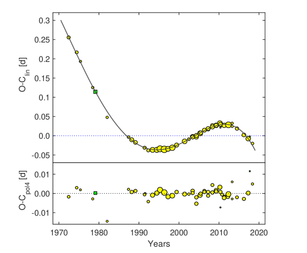
Figure 2: Upper plot: $\mathit{O\!-\!C}_{\rm{lin}}$ versus time in years. $O$ is the moment of the zero phase and $C_{\rm{lin}}=M_{01}+P_{1}\times E$. $M_{01}$ and $P_{1}$ are the parameters of the linear approximation of $O(E)$ behavior, $E$ is the number of rotational cycles elapsed from the initial epoch $M_{01}$ and $P_{1}$ is the mean rotational period in the interval 1970–2018; $M_{01}=2\,452\,650.9048$ and $P_{1}=0.52070819$ d. Nonlinearity of $\mathit{O\!-\!C}_{\rm{lin}}$ is a result of variable rotational period $P$. $\mathit{O\!-\!C}_{\rm{lin}}$ is fitted by a fourth-order polynomial (solid line). Bottom plot: The residuals $\mathit{O\!-\!C}_{\rm{pol4}}$ show that the model ensures the accuracy of ephemeris $0.0025\,\text{d}$ or $0.005$ in phase. Optical photometry is denoted using yellow circles and UV spectrophotometry derived from observed fluxes using green squares. Sizes of the symbols are inversely proportional to the square root of the uncertainties of the determinations of $O$ times derived from individual data sources.

Table 2: Parameters of CU Vir ephemeris (Eq. (4)).

$M_{0}$	(HJD)	2 452 650.8991(6)
$P_{0}$	[d]	0.520 716 59(8)
$\overset{\mathrm{\raisebox{-0.6458pt}{\hbox to0.0pt{\hss$\displaystyle\hskip 1.00006pt.$\hss}}}}{P}_{0}$		4.9(2)$\,\times\,10^{-10}$
$\overset{\mathrm{\raisebox{-0.6458pt}{\hbox to0.0pt{\hss$\displaystyle\hskip 1.00006pt..$\hss}}}}{P}_{0}$	$[\mathrm{d}^{-1}]$	$-1.762(11)\,\times\,10^{-12}$
$\overset{\mathrm{\raisebox{-0.6458pt}{\hbox to0.0pt{\hss$\displaystyle\hskip 1.00006pt...$\hss}}}}{P}_{0}$	$[\mathrm{d}^{-2}]$	$-3.23(5)\,\times\,10^{-16}$

The primary purpose of the proposed definition of the phase function model is finding as simple as possible ephemeris guaranteeing the accuracy in the phase of at least 0.01 in 1970 – 2018. In this time interval, there were obtained 36 129 photometric observations or photometric measurements derived from UV spectra taken by IUE and HST. The data create 177 individual light curves in 37 filters, covering substantial part of CU Vir electromagnetic spectrum. This volume of data is quite sufficient for approximation of the dimensionless phase curve $\vartheta(t)$ and its inversion function $\theta(\vartheta)$ (with a time dimension) by the fourth order polynomial in the form of the Taylor decomposition:

$$\vartheta_{0}=\textstyle{\frac{t-M_{0}}{P_{0}}};\quad\vartheta=\vartheta_{0}-\textstyle{\frac{1}{2!}}\overset{\mathrm{\raisebox{-0.6458pt}{\hbox to0.0pt{\hss$\displaystyle\hskip 1.00006pt.$\hss}}}}{P}_{0}\vartheta_{0}^{2}-\textstyle{\frac{1}{3!}}P_{0}\overset{\mathrm{\raisebox{-0.6458pt}{\hbox to0.0pt{\hss$\displaystyle\hskip 1.00006pt..$\hss}}}}{P}_{0}\vartheta_{0}^{3}-\textstyle{\frac{1}{4!}}P_{0}^{2}\overset{\mathrm{\raisebox{-0.6458pt}{\hbox to0.0pt{\hss$\displaystyle\hskip 1.00006pt...$\hss}}}}{P}_{0}\vartheta_{0}^{4};$$

$$\theta(\vartheta)\!=\!M_{0}\!+\!P_{0}\vartheta\!+\!\textstyle{\frac{1}{2!}}P_{0}\overset{\mathrm{\raisebox{-0.6458pt}{\hbox to0.0pt{\hss$\displaystyle\hskip 1.00006pt.$\hss}}}}{P}_{0}\vartheta^{2}+\textstyle{\frac{1}{3!}}P_{0}^{2}\overset{\mathrm{\raisebox{-0.6458pt}{\hbox to0.0pt{\hss$\displaystyle\hskip 1.00006pt..$\hss}}}}{P}_{0}\vartheta^{3}\!+\!\textstyle{\frac{1}{4!}}P_{0}^{3}\overset{\mathrm{\raisebox{-0.6458pt}{\hbox to0.0pt{\hss$\displaystyle\hskip 1.00006pt...$\hss}}}}{P}_{0}\vartheta^{4};$$ (4)

$$\varphi=\mathrm{frac}({\vartheta});\quad E=\mathrm{floor}({\vartheta});$$ (5)

$$P(t)\doteq P_{0}+P_{0}\,\overset{\mathrm{\raisebox{-0.6458pt}{\hbox to0.0pt{\hss$\displaystyle\hskip 1.00006pt.$\hss}}}}{P}_{0}\,\vartheta_{0}+\textstyle{\frac{1}{2!}}P_{0}^{2}\,\overset{\mathrm{\raisebox{-0.6458pt}{\hbox to0.0pt{\hss$\displaystyle\hskip 1.00006pt..$\hss}}}}{P}_{0}\,\vartheta_{0}^{2}+\textstyle{\frac{1}{3!}}P_{0}^{3}\overset{\mathrm{\raisebox{-0.6458pt}{\hbox to0.0pt{\hss$\displaystyle\hskip 1.00006pt...$\hss}}}}{P}_{0}\vartheta_{0}^{3},$$ (6)

where $\vartheta_{0}$ is an auxiliary dimensionless quantity, $M_{0}$ is the origin of phase function, which was placed close to the weighted center of the observations, $P_{0},\,\overset{\mathrm{\raisebox{-0.6458pt}{\hbox to0.0pt{\hss$\displaystyle\hskip 1.00006pt.$\hss}}}}{P}_{0},\,\overset{\mathrm{\raisebox{-0.6458pt}{\hbox to0.0pt{\hss$\displaystyle\hskip 1.00006pt..$\hss}}}}{P}_{0},$ and $\overset{\mathrm{\raisebox{-0.6458pt}{\hbox to0.0pt{\hss$\displaystyle\hskip 1.00006pt...$\hss}}}}{P}_{0}$ are the instantaneous period and its time derivatives up to third degree at the time $t=M_{0}$, $\varphi$ is the usual phase, and $E$ is the epoch. We selected the Taylor expansion (4) as, contrary to the harmonic expansion (Krtička et al. 2017), it allowed us to directly calculate the phase and its inversion. Using relations in Eqs. (4) and (5) we can calculate the phase function $\vartheta$, the epoch $E$, and the phase $\varphi$, for any HJD moment $t$ within the interval 1972 – 2020. Alternatively, knowing the particular phase function $\vartheta$ we can estimate corresponding time $\theta(\vartheta)$. Changes of the instantaneous period $P(t)=P(\vartheta_{0})$ can be evaluated for any time $t$ using relation (6).

3.3 Model solution and brief discussion of results

All 259 free parameters of our phenomenological model of CU Vir light curves and their corresponding uncertainties were determined together by robust regression (RR) as implemented in Mikulášek et al. (2003), which exploits the well-established procedures of the standard weighted least squares method and eliminates the influence of outliers. Instead of the usual $\chi^{2}$, we minimized the modified quantity $\chi^{2}_{\rm r}$, defined as follows:

$$\Delta y_{i}=y_{i}-F(t_{i},\boldsymbol{\gamma}),$$ (7)

$$\chi^{2}_{\rm r}=\sum_{i=1}^{n}\,\left(\frac{\Delta y_{i}}{\sigma_{\mathrm{r}i}}\right)^{2};\quad\mathrm{where}\ \ \sigma_{\mathrm{r}i}=\sigma_{i}\ \exp\left[\frac{1}{2}\left(\frac{\Delta y_{i}}{4\,\sigma_{i}}\right)^{4}\right],$$ (8)

$$\chi^{2}_{\mu}=1.06\ \frac{\chi^{2}_{\mathrm{r}}}{n_{\rm r}-g};\quad\mathrm{where}\ \ n_{\rm r}=1.02\ \frac{\sum\,\sigma_{\mathrm{r}i}^{-2}}{\sum\,{\sigma_{i}}^{-2}},$$ (9)

$$\delta\gamma_{k}=\sqrt{\chi^{2}_{\mu}\,\mathbb{H}_{kk}},$$ (10)

where $\Delta y_{i}$ is the difference between the observed $i$-th measurement $y_{i}$ and the model prediction $F(t_{i},\boldsymbol{\gamma})$, which is the function of the time of the measurement $t_{i}$ and the vector of the free model parameter $\boldsymbol{\gamma}$, $\sigma_{i}$ is the estimate of the uncertainty of determination of the $i$-th measurement, while $\sigma_{\mathrm{r}i}$ is a RR modified value of $\sigma_{i}$. The estimate of the common relative $\chi^{2}_{\mu}$ and the number of measurements without outliers $n_{\rm r}$ are given by Eq. (9).

The formal uncertainties of the found parameters $\delta\boldsymbol{\gamma}$ were determined by the relation Eq. (10), where $\mathbb{H}$ is a covariant matrix of the system of equations. The most interesting parameters and their functions are listed in Table 2.

The comparison between observation and model predictions in Fig. 2 undoubtedly documents the high fidelity of the chosen model, which yields the phase function ephemeris describing observations with the accuracy better than 0.005 in the interval 1972–2018. The derived period variations can be adequately fitted also by the harmonic polynomials instead of the Taylor expansion (4) and interpreted as due to the torsional oscillations (Krtička et al. 2017).

4 Variations of the UV spectrum

4.1 Simulation of the spectral variability

Table 3: CU Vir parameters from spectroscopy.

Kuschnig et al. 1999
Effective temperature ${{T}_{\mathrm{eff}}}$	${13\,000}$ K
Surface gravity ${\log g}$ (cgs)	${4.0}$
Inclination ${i}$	${30^{\circ}}$
Helium abundance	$-3.2<\varepsilon_{\text{He}}<-1$
Silicon abundance	$-4.6<\varepsilon_{\text{Si}}<-2.3$
Chromium abundance	$-6.7<\varepsilon_{\text{Cr}}<-4.4$
Iron abundance	$-5.5<\varepsilon_{\text{Fe}}<-3.5$
Kochukhov et al. 2014
Effective temperature ${{T}_{\mathrm{eff}}}$	${12\,750}$ K
Surface gravity ${\log g}$ (cgs)	${4.3}$
Radius $R_{*}$	$2.06\,R_{\odot}$
Mass $M$	$3.06\,M_{\odot}$
Inclination ${i}$	${46.5^{\circ}}$
Silicon abundance	$-5.7<\varepsilon_{\text{Si}}<-2.3$
Iron abundance	$-4.7<\varepsilon_{\text{Fe}}<-3.1$

The calculation of the model atmospheres and spectra is the same as described in Paper I. We used the TLUSTY code for the model atmosphere calculations (Hubeny 1988; Hubeny & Lanz 1992, 1995; Lanz & Hubeny 2003) with the atomic data taken from Lanz & Hubeny (2007). In particular, the atomic data for silicon and iron are based on Mendoza et al. (1995), Butler et al. (1993), Kurucz (1994), Nahar (1996), Nahar (1997), Bautista & Pradhan (1997), and Bautista (1996), and for other elements on Luo & Pradhan (1989), Fernley et al. (1999), Tully et al. (1990), Peach et al. (1988), Hibbert & Scott (1994), and Nahar & Pradhan (1993). We prepared our own ionic models for chromium (Cr ii–Cr v) using data taken from Kurucz (2009).

We used two different sets of surface abundance maps. Kuschnig et al. (1999) derived abundance maps of helium, magnesium, silicon, chromium, and iron. Kochukhov et al. (2014) derive abundance maps of silicon and iron only, but using an updated version of the inversion code that accounts also for the magnetic field. For each set of maps (from Kuschnig et al. (1999) and Kochukhov et al. (2014)) we adopted corresponding effective temperatures and surface gravities derived from spectroscopy (see Table 3) and assumed the range of abundances that covers values in individual maps as given in Table 3. Here the abundances are given relative to hydrogen, that is, $\varepsilon_{\text{el}}=\log\left(N_{\text{el}}/N_{\text{H}}\right)$. We neglected the influence of inhomogeneous surface distribution of magnesium due to its low abundance. For each set of maps we used inclination that was derived from corresponding mapping (see Table  3). We used the solar abundance of other elements (Asplund et al. 2005).

For the calculation of synthetic spectra we used the SYNSPEC code. The spectra were calculated for the same parameters (effective temperature, surface gravity, and chemical composition) as the model atmospheres. We also took into account the same transitions (bound-bound and bound-free) as for the model atmosphere calculations. This is important for iron line transitions, for which many lines without experimental values significantly influence the spectral energy distribution. The remaining line data are taken from the line lists available at the TLUSTY web page. We computed emergent specific intensities for $20$ equidistantly spaced values of $\mu=\cos\theta$, where $\theta$ is the angle between the normal to the surface and the line of sight.

The model atmospheres and the emergent specific intensities $I(\lambda,\theta,\varepsilon_{\text{He}},\varepsilon_{\text{Si}},\varepsilon_{\text{Cr}},\varepsilon_{\text{Fe}})$ were calculated for a four-parametric grid of helium, silicon, chromium, and iron abundances (see Table 4). The lowest abundances of individual elements are omitted from the grid. Our test showed that this restriction does not influence the predicted light curves.

Table 4: Individual abundances $\varepsilon_{\text{He}}$, $\varepsilon_{\text{Si}}$, $\varepsilon_{\text{Cr}}$, and $\varepsilon_{\text{Fe}}$ of the model grid.

He	$-2.0$	$-1.0$
Si	$-4.75$	$-4.25$	$-3.75$	$-3.25$	$-2.75$	$-2.25$
Cr	$-6.4$	$-5.9$	$-5.4$	$-4.9$	$-4.4$
Fe	$-5.4$	$-4.9$	$-4.4$	$-3.9$	$-3.4$	$-3.1$

The radiative flux at the distance $D$ from the star with radius $R_{*}$ is (Hubeny & Mihalas 2014)

$$F_{\lambda}=\left(\frac{R_{*}}{D}\right)^{2}\!\!\int\limits_{\begin{array}[]{c}\text{\scriptsize visible}\\[-5.69054pt] \text{\scriptsize surface}\end{array}}\!\!I(\lambda,\theta,\Omega)\cos\theta\,\text{d}\Omega.$$ (11)

The intensity $I(\lambda,\theta,\Omega)$ at each surface point with spherical coordinates $\Omega$ is obtained by means of interpolation between the emergent specific intensities $I(\lambda,\theta,\varepsilon_{\text{He}},\varepsilon_{\text{Si}},\varepsilon_{\text{Cr}},\varepsilon_{\text{Fe}})$ calculated from the grid of synthetic spectra (Table 4) taking into account the Doppler shifts due to the stellar rotation.

4.2 Comparison with the observed variations

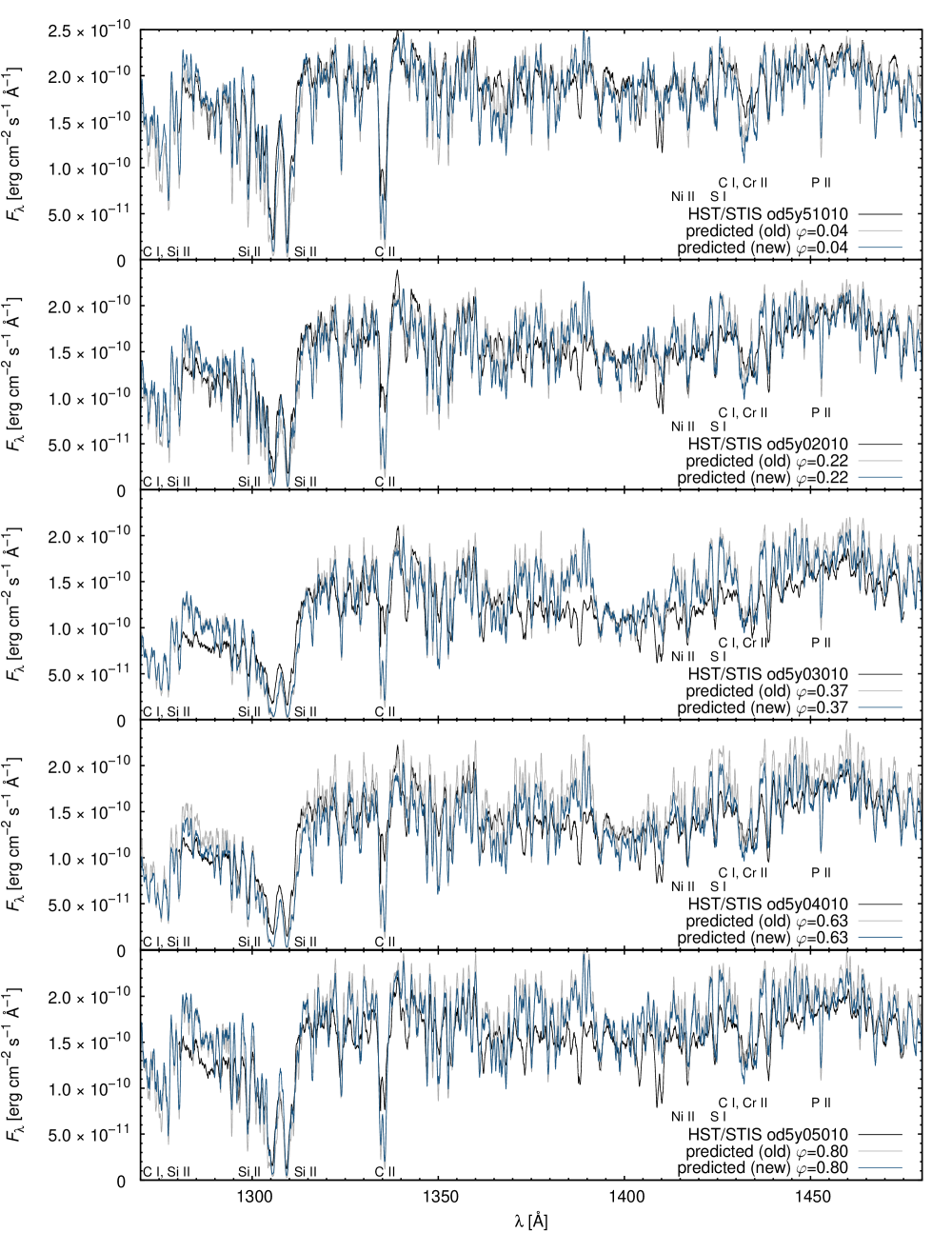
Figure 3: Predicted and observed (HST, black line) flux in selected phases for the wavelength range 1270 – 1480 Å. The gray line denotes spectra calculated using Kuschnig et al. (1999) surface abundance distribution and blue line denotes spectra calculated using Kochukhov et al. (2014) surface abundance distribution. Individual strong lines and iron line blends are identified.

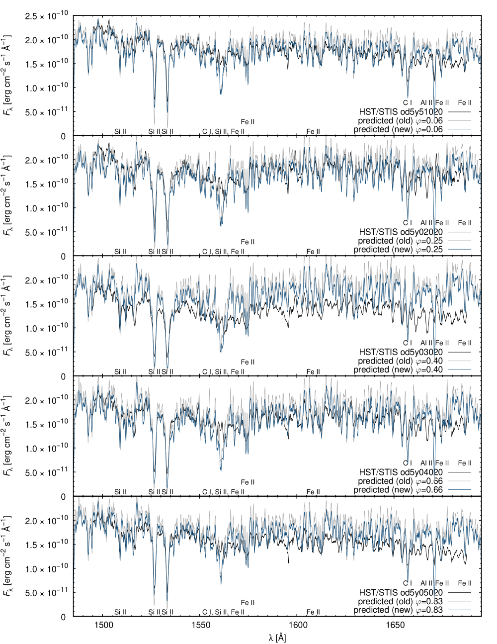
Figure 4: Same as Fig. 3, except for the wavelength range 1485 – 1695 Å.

We compared flux variations predicted using Eq. (11) with flux variations observed by HST/STIS for individual rotational phases $\varphi$. The predicted fluxes were scaled by the $(R_{*}/D)^{2}$ ratio derived in Paper I from the IUE spectra.

The fluxes calculated from the two sets of abundance maps show a good agreement with observed spectra for the spectral region around 1280 – 1475 Å (see Fig. 3) especially for the rotational phase $\varphi\approx 0$, when the regions with low abundance of iron and silicon are visible. This spectral region is dominated by silicon bound-free and iron line transitions.

The two sets of abundance maps provide similar results for the 1494 – 1688 Å wavelength region, where the influence of silicon is weaker (see Fig. 4). The predicted fluxes nicely agree with observations for phases $\varphi\approx 0$ and $\varphi\approx 0.2$, while the predicted fluxes are slightly larger than the observations for $\varphi\approx 0.4$, $\varphi\approx 0.6$, and $\varphi\approx 0.8$. A detailed inspection of fluxes shows that the new maps agree with observations even slightly better during the phases $\varphi\approx 0$, $\varphi\approx 0.2$, and $\varphi\approx 0.6$ in the interval $1600-1650\,$Å. The remaining disagreement is likely caused by missing opacity due to some additional element(s). We tested the flux distribution calculated with enhanced abundance of light elements with $Z<30$ and we have found that a missing opacity is possibly due to chromium. The predicted flux distribution for $\epsilon_{\text{Cr}}=-4$ nicely matches the observations for $\varphi\approx 0.4$. Chromium was mapped by Kuschnig et al. (1999), but new maps based on more detailed spectroscopy could possibly give higher chromium abundance in the spots.

We also tested new line data from the VALD database (Piskunov et al. 1995; Kupka et al. 1999; Ryabchikova 2015). This led to an improvement of the agreement in some specific lines, but caused disagreement in others. Consequently, part of the discrepancy between the predicted and observed spectra can be probably attributed to the imprecise line data.

In addition to the line variability of elements studied in optical (silicon, chromium, and iron), the UV spectra also show carbon line variability. Carbon is roughly depleted by a factor of ten with respect to the solar value, consequently it is not expected to significantly affect the flux distribution. We also tested the presence of lines of heavy elements, with atomic number $Z\leq 92$, in the spectra of CU Vir. We used our original line list and the line list downloaded from the VALD database (Piskunov et al. 1995; Kupka et al. 1999; Ryabchikova 2015). We find no evidence for the presence of lines of elements having $Z>30$ in the spectra of CU Vir.

5 Stellar wind of CU Vir

The explanation of CU Vir continuum radio emission by gyrosynchrotron process requires a wind mass-loss rate on the order of $10^{-12}\,{M}_{\odot}\,\text{yr}^{-1}$ (Leto et al. 2006). However, wind models show that the radiative force is too weak to accelerate the wind for CU Vir’s effective temperature (Krtička 2014). To understand this inconsistency, we provide additional wind tests and search for the wind signatures in the CU Vir spectra.

We used our METUJE wind code (Krtička 2014) to test if the radiative force overcomes gravity in the envelope of CU Vir and to calculate the wind spectra. Our wind code solves the hydrodynamic equations (equations of continuity, motion, and energy) in a stationary spherically symmetric stellar wind. The radiative transfer equation is solved in the comoving frame (CMF). The code allows us to treat the atmosphere and wind in a unified (global) manner (Krtička & Kubát 2017), but for the present purpose we modeled just the wind with the METUJE code, and we derived the base flux from the TLUSTY model atmosphere model with $\epsilon_{\text{He}}=-1$, $\epsilon_{\text{Si}}=-3.25$, $\epsilon_{\text{Cr}}=-5.4$, and $\epsilon_{\text{Fe}}=-3.1$. To enable better comparison with the observed spectra, the TLUSTY flux in the regions of strong wind lines was replaced by the flux predicted from inhomogeneous surface abundances for phase $\varphi=0.30$.

For the wind tests, we assumed fixed wind density and velocity and compared the radiative force with gravity (Krtička 2014). We tested mass-loss rates in the range of $10^{-14}-10^{-10}\,{M}_{\odot}\,\text{yr}^{-1}$ for mass-fractions of the heavy elements $Z$ relative to the solar value $Z_{\odot}$ in the range $Z=Z_{\odot}-10^{3}Z_{\odot}$ scaling abundances of all elements heavier than helium by the same value. The radiative force is typically one or two orders of magnitude lower than the gravitational acceleration (in absolute values). The radiative force overcomes gravity only for the most metal rich model with $Z=10^{3}Z_{\odot}$, which is higher than the fraction of silicon and iron found in metal rich regions on the CU Vir surface (see Table 3). Consequently, we find no wind in CU Vir from our theoretical models. This is consistent with results of Babel (1996), who also found no wind for stellar parameters corresponding to CU Vir. A weak, purely metallic wind with $\overset{\mathrm{\raisebox{-0.6458pt}{\hbox to0.0pt{\hss$\displaystyle\hskip 1.00006pt.$\hss}}}}{M}\approx 10^{-16}\,{M}_{\odot}\,\text{yr}^{-1}$ is still possible for such low-luminosity stars (Babel 1995).

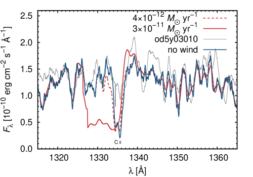
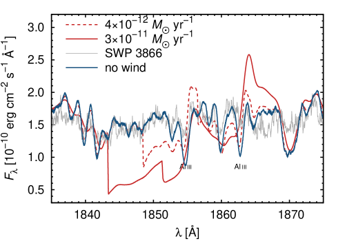
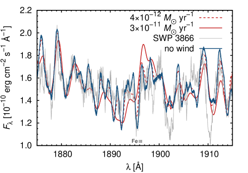
Figure 5: Predicted wind spectra for two values of mass-loss rates (red lines) in comparison with spectra without wind (blue line) and observed spectra (gray line).

Spectral lines originating in the wind have in general complex line profiles, which depend on the wind mass-loss rate, velocity law, and ionization balance. Especially at low wind densities, the wind line profiles could be hidden in blends of numerous UV lines. Therefore, to determine which wind lines could possibly be found in the observations, we used our METUJE code to predict the wind spectra. We assumed $Z=10^{2}Z_{\odot}$, which roughly corresponds to the most silicon and iron rich surface layers and artificially multiplied the radiative force by a factor of 3–10 to get wind model to converge with different wind mass-loss rates. Below we discuss further two representative wind models with a mass-loss rate $\overset{\mathrm{\raisebox{-0.6458pt}{\hbox to0.0pt{\hss$\displaystyle\hskip 1.00006pt.$\hss}}}}{M}=4\times 10^{-12}\,{M}_{\odot}\,\text{yr}^{-1}$ and terminal velocity $v_{\infty}=1010\,\text{km}\,\text{s}^{-1}$ and a model with $\overset{\mathrm{\raisebox{-0.6458pt}{\hbox to0.0pt{\hss$\displaystyle\hskip 1.00006pt.$\hss}}}}{M}=3\times 10^{-11}\,{M}_{\odot}\,\text{yr}^{-1}$ and $v_{\infty}=1850\,\text{km}\,\text{s}^{-1}$.

We find that the strongest wind features appear in the C ii lines at 1335 Å and 1336 Å and in the Al iii lines at 1855 Å and 1863 Å (Fig. 5). Aluminum lines are predicted to show strong absorption and emission in P Cygni profiles. The absorption is weaker in the model with lower mass-loss rate and less blue-shifted as a result of lower wind terminal velocity. The carbon lines show P Cygni profiles with slightly extended absorption and show emission only for the highest mass-loss rates considered. These lines become weaker close to the blue edge of the P Cygni line profile due to C ii ionization. There are no such features in the observed spectra of CU Vir. If the assumed abundances are correct, this would limit the CU Vir mass-loss rate to $\overset{\mathrm{\raisebox{-0.6458pt}{\hbox to0.0pt{\hss$\displaystyle\hskip 1.00006pt.$\hss}}}}{M}\lesssim 10^{-12}\,{M}_{\odot}\,\text{yr}^{-1}$, below the value required to explain the radio emission (Leto et al. 2006). On the other hand, the photospheric components of C and Al lines show that these elements are likely underabundant (similarly to carbon on the surface of $\sigma$ Ori E, Oksala et al. 2015). In such a case the wind lines of these elements would not be present in the spectra and the imposed wind limit should be higher.

Therefore, we concentrated on the wind lines of silicon and iron, the two elements which are overabundant on the surface of CU Vir. The 1394 Å and 1403 Å lines of Si iv, which might be relatively strong in the spectra of stars with slightly higher effective temperature (Krtička 2014), do not appear in the CU Vir spectra due to silicon recombination. Therefore, the strongest limit to the mass-loss rate comes from the absence of Fe iii 1895 Å wind line in Fig. 5, which gives $\overset{\mathrm{\raisebox{-0.6458pt}{\hbox to0.0pt{\hss$\displaystyle\hskip 1.00006pt.$\hss}}}}{M}\lesssim 10^{-11}\,{M}_{\odot}\,\text{yr}^{-1}$.

Spectra in Fig. 5 are plotted for a particular phase $\varphi\approx 0.3$. In magnetic stars, the wind properties depend on the tilt of the magnetic field (e.g., ud-Doula et al. 2009), therefore, the wind line profiles show rotational variability (Bjorkman et al. 1994; Marcolino et al. 2013; Nazé et al. 2015). We tested the existence of the wind also in other phases with similar conclusions as for the phase $\varphi\approx 0.3$. Consequently, we conclude that the presence of the stellar wind in CU Vir can not be proven even from our spectra with the highest quality. This corresponds to observation of very weak wind lines in early-type magnetic stars (Oskinova et al. 2011). These lines give the mass-loss rate on the order of $10^{-11}-10^{-10}\,{M}_{\odot}\,\text{yr}^{-1}$, but for stars whose luminosity is nearly two magnitudes higher. Given a strong dependence of mass-loss rate on luminosity, the upper limit of the CU Vir mass-loss rate is not surprising.

There are additional possible wind indicators in the wavelength region between the Lyman jump and Ly$\alpha$ line. The 1086 Å N ii line is predicted to show nice P Cygni line profile, but it is located in the region where the model flux is roughly one order of magnitude lower than the flux in the 1300–1400 Å region. The lines 1176 Å C iii and 1206 Å Si iii are located in the wavelength region covered by the IUE observations, but the observed flux is rather noisy. In any case, the observed spectra in the region of 1206 Å Si iii are consistent with the $10^{-11}\,{M}_{\odot}\,\text{yr}^{-1}$ limit of the mass-loss rate.

CU Vir has relatively strong magnetic field, which may affect the calculation of the radiative force and wind line profiles (e.g., Shenar et al. 2017). The wind lines originate in the magnetosphere with a complex structure leading to the dependence of wind line profiles on phase and inclination (e.g., Marcolino et al. 2013). The plasma effects become important in the wind at low densities and the wind behaves as a multicomponent flow (Krtička & Kubát 2002). Moreover, at low densities the shock cooling length is comparable to the radial wind scale, possibly causing weak wind line profiles (Cohen et al. 2008; Krtička & Kubát 2009; Lucy 2012). We tested the inclusion of complete photoionization cross-sections for Si ii – Si iii (with autoionization resonances, Butler et al. 1993). This has not lead to a significant increase of the radiative force, but there may still be some elements missing in our list (Krtička & Kubát 2009) that are overabundant on CU Vir’s surface and may drive a wind. Moreover, wind inhomogeneities (clumping) affect wind ionization state and wind line profiles (Sundqvist et al. 2010; Šurlan et al. 2012). Although Oskinova et al. (2011) finds no significant differences in the spectra of clumped and smooth stellar wind for their particular model of B star, there might still be significant effects of clumping for other stellar parameters. Therefore, there still might be possibilities to launch stellar wind in CU Vir that does not show any signatures in UV spectra, but at the moment there is no theoretical nor observational support for the existence of the stellar wind in CU Vir.

6 Search for auroral lines

The radio emission in CU Vir originates due to processes resembling auroral activity in Earth and giant planets (Trigilio et al. 2011). Therefore, we searched for auroral lines in the UV spectra of CU Vir. Because the auroral lines originate from the rigidly rotating magnetosphere, we expect these lines to be broadened by at least $v_{\text{rot}}\sin i=145\,\text{km}\,\text{s}^{-1}$, which corresponds to the projected equatorial rotational velocity (Kochukhov et al. 2014). Moreover, the auroral lines would likely show rotational variability as a result of complex structure of the magnetosphere.

Table 5: Lines searched in CU Vir spectra for auroral emission.

Ion	Lines [Å]
He ii	1640
C i	1330, 1561, 1657
C ii	1335
O i	1302, 1305, 1306, 1356, 1359
Si i	1556 – 1675
Si ii	1305, 1309, 1527, 1533
P i	1381
P ii	1533, 1536, 1542, 1543, 1544
S i	1283 – 1475
Cl i	1347, 1352
Ti iii	1282 – 1300
Fe ii	1559 – 1686
Co ii	1448, 1456, 1466. 1473, 1509, 1548
Ni ii	1317, 1335, 1370, 1411
Cu ii	1359

The planetary auroral emission comprises molecular lines (e.g., Soret et al. 2016; Gustin et al. 2017), which are not expected in CU Vir due to its high temperature. We searched for the auroral emission of neutral oxygen lines given in Table 5, which are detected in planetary magnetospheres (e.g., Molyneux et al. 2014; Soret et al. 2016). The lower level of all these lines corresponds to the ground state. We find no auroral lines of neutral ions. This is not surprising, as our wind models indicate that the magnetosphere is dominated by singly and doubly ionized elements.

Therefore, we also searched for the auroral emission in lines whose lower level corresponds to the ground state of singly and doubly ionized elements (see Table 5). We did not find any emission line profiles that can be attributed to the circumstellar medium, either. However, this does not necessary mean that there are no such lines present in the available spectra. Given the complexity and variability of photospheric spectra, the auroral lines may remain overlooked.

Some hot white dwarfs show ultra-high excitation absorption lines in their spectra (e.g., Werner et al. 1995; Dreizler et al. 1995; Reindl et al. 2019). These lines possibly originate in shock-heated magnetospheres of white dwarfs. Such a process can also appear in magnetic main-sequence stars. We searched for these lines in the optical spectra of CU Vir, but we have not found any.

7 Lines of interstellar medium

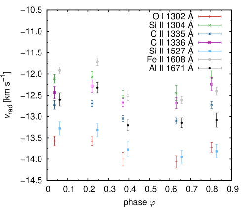
Figure 6: Variation of the radial velocity shift of the interstellar lines with phase. Derived from $\delta\lambda$ parameter of the fit (12) using the Doppler law.

HST/STIS spectra of CU Vir show several interstellar lines, which are missing in Figs. 3 and 4 due to the application of median filter. We studied the variability of interstellar lines in the original spectra downloaded from MAST archive. For this purpose we fitted the individual interstellar lines by

$$F(\lambda)=(F_{0}+F_{1}\lambda)\exp\left\{-s\exp\left[-\left(\frac{\lambda-\lambda_{0}-\delta\lambda}{d}\right)^{2}\right]\right\},$$ (12)

which is a solution of the radiative transfer equation in a uniform medium with Gaussian line absorption. Parameters $F_{0}$ and $F_{1}$ account for the stellar continuum, $\lambda_{0}$ is the laboratory wavelength of a given line, and $s$, $\delta\lambda$, and $d$ are parameters of the fit.

We identify individual interstellar lines using the list provided by Cox (2000). We fitted them by line profile function Eq. (12) and searched for the phase variability of the line parameters. We find phase variability of the line shift $\delta\lambda$ (see Fig. 6), which is correlated with line width parameter $d$ in both STIS bands.

Table 6: Parameters of the fit Eq. (12) of individual interstellar lines.

Line	$\delta\lambda$ [mÅ]	$d$ [mÅ]
O i 1302 Å	$-59.9\pm 0.8$	$23.8\pm 1.4$
Si ii 1304 Å	$-53.3\pm 0.8$	$19.2\pm 1.1$
C ii 1335 Å	$-57.3\pm 0.7$	$28.0\pm 0.7$
C ii 1336 Å	$-55.5\pm 0.7$	$13.6\pm 0.4$
Si ii 1527 Å	$-69.4\pm 1.2$	$24.4\pm 0.7$
Fe ii 1608 Å	$-65.6\pm 1.6$	$15.4\pm 0.5$
Al ii 1671 Å	$-71.7\pm 1.7$	$22.6\pm 0.5$

It is tempting to attribute these variations to circumstellar clouds that amplify the interstellar absorption. The centrifugally supported circumstellar clouds can exist above the radius where the centrifugal force overcomes gravity $r=\left[GMP^{2}/\left(4\pi^{2}\right)\right]^{1/3}$ (Townsend & Owocki 2005), which for the stellar parameters given in Table 3 gives $r=1.9\,R_{*}$. This is at odds with estimated temperature of the clouds. The Si ii 1533 Å line with lower-level excitation energy 0.036 eV is not present in the spectrum, while C ii 1336 Å line with lower-level excitation energy 0.008 eV is clearly visible. This implies the temperature of absorbing medium on the order of 10 K, which cannot be achieved in a close proximity of the star. Moreover, the expected rotational line broadening due to rigidly rotating centrifugal magnetosphere, which is at least equal to the surface rotational velocity $v_{\text{rot}}\sin i=145\,\text{km}\,\text{s}^{-1}$ (Kochukhov et al. 2014), is an order of magnitude higher than the observed broadening of interstellar lines. The difference between the shift estimated from the spectra centered at 1380 Å and spectra centered at 1598 Å around the phase $\varphi\approx 0.8$ (Fig. 6) is comparable to the uncertainty of $\delta\lambda$. Finally, the unsaturated C ii 1336 Å line shows the same variability as saturated lines implying comparable absorption due to both the interstellar medium and to the putative circumstellar cloud. Consequently, we conclude that the line variability in Fig. 6 does not originate in the centrifugal magnetosphere and that it is likely generated further out from the star.

We also tested the possibility that the interstellar line variability is a result of a constant circumstellar absorption acting on variable flux. For this purpose we used simulated spectra attenuated by circumstellar line absorption and fitted the resulting spectra by Eq. (12). We detected only order of magnitude smaller variations than those derived from observations. Consequently, the observed variations of the interstellar medium lines are most likely only of instrumental origin. Although the STIS spectrograph provides subpixel wavelength stability (i.e., leading to lower changes than that seen in Fig. 6, Riley et al. 2018), subsequent processing of variable spectra likely leads to larger differences. We therefore simply averaged the radial velocities inferred from Table 6 to get the mean radial velocity of the interstellar medium of $-12.9\pm 0.4\,\text{km}\,\text{s}^{-1}$. Because CU Vir is located close to the rim of the Spica Nebula, which results from the interaction of the Local Bubble with another interstellar bubble (Choi et al. 2013), the interstellar lines in CU Vir spectra may be connected with these structures.

8 Discussion: Tracing the wind

The upper limit for the wind mass-loss rate $10^{-12}\,M_{\odot}\,\text{yr}^{-1}$ is in tension with the mass-loss rate on the order of $10^{-12}\,M_{\odot}\,\text{yr}^{-1}$ required to explain the CU Vir radio emission (Leto et al. 2006). This estimate was derived assuming the balance between the ram pressure of the wind and the plasma pressure in the inner magnetosphere. On the other hand, leaving this requirement and assuming instead that the magnetospheric plasma is in hydrostatic equilibrium (Townsend & Owocki 2005) allows for much lower wind mass-loss rate required to feed the magnetosphere. Within such a model, even the pure metallic wind predicted by Babel (1996) might be strong enough to power the radio emission.

In contrast, even relatively strong wind is consistent with the angular momentum loss via the magnetized stellar wind. This mechanism affects the rotational velocities of early-B stars (Shultz et al. 2017) and should be present also in late-B stars with winds. Assuming $\overset{\mathrm{\raisebox{-0.6458pt}{\hbox to0.0pt{\hss$\displaystyle\hskip 1.00006pt.$\hss}}}}{M}=10^{-12}\,{M}_{\odot}\,\text{yr}^{-1}$, a typical wind terminal velocity $v_{\infty}=1000\,\text{km}\,\text{s}^{-1}$, dipolar magnetic field strength of CU Vir $B_{\text{p}}=3\,\text{kG}$ (Kochukhov et al. 2014), and angular momentum constant $k=0.08$ as derived from MESA models (Paxton et al. 2011, 2013, see Krtička et al. 2017 for details) we derive from Eq. (25) of ud-Doula et al. (2009) the spin-down time $1.4\times 10^{8}\,\text{yr}$, which is consistent with an estimated age $\leq 100\,\text{Myr}$ of CU Vir (Kochukhov et al. 2014).

The stellar wind also likely powers X-ray emission of CU Vir (Robrade et al. 2018). Assuming full conversion of wind kinetic energy to X-rays, then with wind terminal velocity $v_{\infty}=1000\,\text{km}\,\text{s}^{-1}$, a mass-loss rate $10^{-13}\,{M}_{\odot}\,\text{yr}^{-1}$ is required to power the X-ray luminosity $L_{\text{X}}=3\times 10^{28}\,\text{erg}\,\text{s}^{-1}$ derived from the observations. This mass-loss rate is below the upper limit derived here.

It is unclear what drives the supposed torsional oscillations in CU Vir. The properties of the corresponding energy source can be estimated from the total energy of these oscillations, which is given by the kinetic energy density of oscillatory motion integrated over the whole stellar volume,

$$E_{\text{to}}=4\pi\int_{0}^{R_{*}}r^{2}\frac{1}{2}\rho\delta\varv^{2}\,\text{d}r,$$ (13)

where $\delta\varv$ is the velocity amplitude of the oscillations, which is connected with the amplitude of the angular frequency by $\delta\varv=r\delta\Omega$. The surface value of the amplitude of the angular frequency $\delta\Omega_{*}$ can be derived from the harmonic fit of the period variability $P(t)=P_{0}+A\,\sin\left[2\,\pi\left(t-\mathit{\Theta_{0}}\right)/{\mathit{\Pi}}\right]$ (Krtička et al. 2017) as $\delta\Omega_{*}\approx 2\pi A/P_{0}^{2}$. Here $A$ and $\mathit{\Pi}$ are the amplitude and length of the cycle of rotational period evolution. From this, the total energy of the torsional oscillations is

$$E_{\text{to}}=8\pi^{3}\frac{A^{2}}{P_{0}^{4}}\int_{0}^{R_{*}}r^{4}\rho\left(\frac{\delta\Omega}{\delta\Omega_{*}}\right)^{2}\,\text{d}r.$$ (14)

The energy can be conveniently rewritten using the angular momentum constant $k$, and assuming that $\delta\Omega$ does not depend on radius one can get an estimate $E_{\text{to}}=2\pi^{2}kMR^{2}A^{2}/P_{0}^{4}$.

To derive a more precise estimate of the total energy of the torsional oscillations, we used the stellar density distribution from the discussed MESA stellar evolutionary model. We assumed that the amplitude of $\delta\Omega$ is proportional to the amplitude of $u_{1}$ variable for time $t=10\,\mathit{\Pi}$ of torsional oscillation simulations (Krtička et al. 2017, Fig. 1). The selection of a particular time $t$ does not have a significant effect on estimated value of $E_{\text{to}}$. We scaled the numerical solution for $u_{1}$ using the observed variations of rotational period at the stellar surface. These assumptions yield $E_{\text{to}}=5\times 10^{37}\,\text{erg}$, which is just about $5\times 10^{-7}$ of the total energy of X-rays emitted during the whole CU Vir lifetime (assuming constant $L_{\text{X}}$ and an upper limit of CU Vir age, 100 Myr, Kochukhov et al. 2014). Consequently, stellar wind, which presumably powers the X-ray emission, provides a convenient energy source also for the torsional oscillations.

The continuous wind leakage from the magnetosphere is likely not the mechanism that drives the oscillations, but a sudden energy release during the reconnection event that opens up the magnetosphere (Townsend & Owocki 2005) might be more likely. Such events are probably very rare, because the corresponding breakout time is about $10^{5}\,\text{yr}$ as estimated from Eq. (A8) of Townsend & Owocki (2005) for CU Vir parameters.

9 Conclusions

We analyzed the HST/STIS spectra of the enigmatic chemically peculiar star CU Vir. This is the first discovered main-sequence star showing coherent directive radio emission (Trigilio et al. 2000). The existence of such radio emission requires wind with mass-loss rate on the order of $10^{-12}\,{M}_{\odot}\,\text{yr}^{-1}$ as a source of free electrons (Leto et al. 2006). However, the effective temperature of CU Vir is below the limit of homogeneous winds $T_{\text{eff}}\approx 15\,000\,$K (Krtička 2014). Our analysis of UV spectra of the star has not revealed any wind signatures and puts the upper limit of CU Vir mass-loss rate at about $10^{-12}\,{M}_{\odot}\,\text{yr}^{-1}$. Although the physics of low density winds is complex and there are reasons for even stronger winds to remain hidden from UV analysis, we argue that even weaker inhomogeneous (metallic) wind of Babel (1996) may be a reasonable source of free electrons to power the radio and X-ray emission of CU Vir.

We searched for other signatures of magnetospheric plasma including auroral emission lines and deep absorption lines. However, we have not found any signatures that can be attributed to magnetospheric plasma.

CU Vir shows long-term rotational period variations (Pyper et al. 1998; Mikulášek et al. 2011). We analyzed these variations using available UV observations supplemented with our own and archival optical photometric data. We concluded that the data from optical and UV domains show the same long-term evolution of the rotational period. This supports the picture that the UV and optical variations are related and that the structures leading to these variations are rigidly confined to the stellar surface.

We modeled the UV flux variability assuming its origin in the surface abundance spots, in which the flux redistribution due to bound-bound and bound-free processes takes place. We show that the updated abundance maps of Kochukhov et al. (2014) provide improved flux distributions that agree better with observations mainly around $1600\,\AA$.