Deep Gaussian Processes for Multi-fidelity Modeling

Abstract

Multi-fidelity methods are prominently used when cheaply-obtained, but possibly biased and noisy, observations must be effectively combined with limited or expensive true data in order to construct reliable models. This arises in both fundamental machine learning procedures such as Bayesian optimization, as well as more practical science and engineering applications. In this paper we develop a novel multi-fidelity model which treats layers of a deep Gaussian process as fidelity levels, and uses a variational inference scheme to propagate uncertainty across them. This allows for capturing nonlinear correlations between fidelities with lower risk of overfitting than existing methods exploiting compositional structure, which are conversely burdened by structural assumptions and constraints. We show that the proposed approach makes substantial improvements in quantifying and propagating uncertainty in multi-fidelity set-ups, which in turn improves their effectiveness in decision making pipelines.

1 Introduction

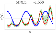
ar1	nargp	mf-dgp

Figure 1: Limitations addressed and resolved jointly by our proposed mf-dgp architecture. Blue and red markers denote low and high-fidelity observations respectively. Shaded regions indicate the 95% confidence interval.

A common issue encountered in active learning procedures such as Bayesian optimization (Shahriari et al., 2016) and experimental design (Morris, 2004) is the difficulty or cost to acquire sufficient data. Constructing a reliable model of the underlying system when only few observations are available is challenging, making it common practice to develop simulators from which data can more easily be obtained. Practical examples include computational fluid dynamics for vehicular engineering (Koziel & Leifsson, 2013), weather simulators for climate modeling (Majda & Gershgorin, 2010), and emulators for reinforcement learning (Cutler et al., 2014).

Multi-fidelity models (Kennedy & O’Hagan, 2000; Peherstorfer et al., 2018) are designed to fuse limited true observations (high-fidelity) with cheaply-obtained lower granularity approximations (low-fidelity). However, naïvely combining data from multiple information sources could result in a model giving predictions which do not accurately reflect the true underlying system. In absence of well-defined information regarding the reliability of each fidelity and the relationships between fidelities, Bayesian inference captures the principle of Occam’s razor through explicitly encoding our uncertainty about these factors (MacKay, 2003). This implicit regularization is pertinent to settings with limited data where overfitting is otherwise likely to occur.

In the spirit of Bayesian modeling, Gaussian processes (gps; Rasmussen & Williams, 2006) are well suited to multi-fidelity problems due their ability to encode prior beliefs about how fidelities are related, yielding predictions accompanied by uncertainty estimates. gps formed the basis of seminal autoregressive models (henceforth ar1) investigated by Kennedy & O’Hagan (2000) and Le Gratiet & Garnier (2014), and were shown to be effective given a linear mapping between fidelities, i.e. the high-fidelity function $f_{t}$ can be modeled as:

$$f_{t}(x)=\rho_{t}f_{t-1}\left(x\right)+\delta_{t}\left(x\right)\text{,}$$ (1)

where $\rho_{t}$ is a constant scaling the contribution of samples $f_{t-1}$ drawn from the gp modeling the data at the preceding fidelity, and $\delta_{t}(x)$ models the bias between fidelities. However, such models are insufficient when the relationship between fidelities is nonlinear, i.e. there is now a space-dependent nonlinear transformation $\rho_{t}$ that relates one fidelity to the next as:

$$f_{t}(x)=\rho_{t}\left(f_{t-1}\left(x\right),x\right)+\delta_{t}\left(x\right).$$ (2)

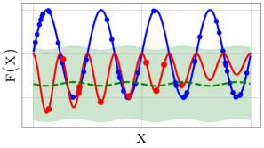
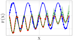
The additive structure and independence assumption between the gps for modeling $\rho_{t}\left(f_{t-1}\left(x\right),x\right)$ and $\delta_{t}\left(x\right)$ permits us to combine these as a single gp that takes as inputs both $x$ and $f^{*}_{t-1}(x)$, where the latter denotes a sample from the posterior of the gp modeling the preceding fidelity evaluated at $x$. This results in a composition of gps that can be compactly expressed as $f_{t}(x)=g_{t}\left(f_{t-1}^{*}\left(x\right),x\right)$. As highlighted by Perdikaris et al. (2017) and exemplified in Figure 1, the ar1 model cannot capture nonlinear correlations between fidelities.

Problem Statement

Deep Gaussian processes (dgps; Damianou & Lawrence, 2013) are a natural candidate for handling nonlinearities between fidelities by way of function composition, allowing for uncertainty propagation in a nested structure of gps where each gp models the transition from one fidelity to the next. However, dgps are cumbersome to develop and approximations are necessary for enabling tractable inference. In spite of being motivated by the structure of dgps, the nonlinear multi-fidelity model (nargp) proposed by Perdikaris et al. (2017) amounts to a disjointed architecture whereby each gp is fitted in an isolated hierarchical manner, thus preventing gps at lower fidelities from being updated once they have already been fit. This deconstruction into independent models which are optimized sequentially violates our aforementioned preference of using Occam’s razor as a means of controlling the model’s complexity, making it more susceptible to overfitting.

Consider the example given in Figure 1. In the tail-end of the function, there are no high-fidelity observations available and only low-fidelity points to fall back on. In this case, we would expect the model to return higher uncertainty to reflect the lack of data available, but instead, nargp predicts an incorrect result with high confidence. Closer inspection of the optimal hyperparameters obtained after training the model confirms our intuition regarding overfitting, since kernel parameters settle at values which are orders of magnitude larger than the range in which they are expected to lie. This is particularly problematic when the model is intended for use in a computational pipeline or active learning procedure, where uncertainty calibration is imperative.

In this work, we propose the first complete interpretation of multi-fidelity modeling using dgps, which we refer to as mf-dgp. In particular, we construct a multi-fidelity dgp model which can be trained end-to-end, overcoming the constraints that hinder existing attempts at using dgp structure for this purpose. Having a dgp model that communicates uncertainty estimates between all fidelities at training time also allows us to properly assess the suitability of dgps over standard gps in the multi-fidelity setting. Returning to the example given in Figure 1, we see that our model fits the true function properly while also returning sensibly conservative uncertainty estimates. Moreover, our model also inherits the compositional structure of nargp, thus alleviating a crucial limitation of the ar1 model. The model’s formulation leverages the sparse dgp approximation proposed by Salimbeni & Deisenroth (2017) for tractability.

Our principal contributions are listed below:

• We identify potential issues with existing approaches for compositional multi-fidelity modeling, emphasising their tendency to overfit;

• We develop a novel multi-fidelity model which enables end-to-end training with well-calibrated uncertainty quantification. This includes a detailed analysis of the nuances involved in its construction;

• We provide a thorough experimental evaluation of our model by way of comparisons with other techniques, application to a large-scale real-world problem, and showcase the use of mf-dgp for experimental design using a determinantal point process;

• The model implementation has been integrated in Emukit, an open-source package for carrying out emulation and decision making in a design loop.

The paper is organized as follows. In the next section, we review the literature on multi-fidelity modeling with gps and clarify how our contributions fit within this landscape. Subsequently, in Section 3 we introduce dgps and illustrate how these can be interpreted in the multi-fidelity setting. A detailed description and discussion of our model, mf-dgp, follows in Section 4, and its performance is evaluated in Section 5, where we also compare our results against a selection of alternatives. An outlook on extensions and future work concludes the paper.

2 Related Work

Multi-fidelity models came to prominence in the foundational work by Kennedy & O’Hagan (2000), where a gp having a kernel suited for multi-fidelity observations was used to model linear correlations between data at $T$ ordered fidelity levels. However, the flexibility of this approach was burdened by the cubic computational complexity associated with gp inference. This led Le Gratiet & Garnier (2014) to propose a recursive multi-fidelity model whereby the observations for each fidelity are modeled using independent gps. Aside from reducing the computational complexity from $\mathcal{O}((\sum_{t=1}^{T}N_{t})^{3})$ to $\mathcal{O}(\sum_{t=1}^{T}N_{t}^{3})$, where $N_{t}$ denotes the number of observations with fidelity level $t$, the posterior obtained from this model was also shown to be identical to that of the original model under the assumptions of noiseless observations and nested inputs, i.e. points observed with fidelity level $t$ are also observed at all lower fidelities.

The similarity between nested gp models for multi-fidelity and traditional deep gps was first noted by Perdikaris et al. (2017) in their formulation of the nargp model, where the parallels to dgp inference are derived from propagating uncertain outputs from one gp to the next. Nonetheless, the design and implementation of our mf-dgp model is markedly different, and this has notable implications on both the model architecture as well as its predictive performance. Whereas nargp amounts to a set of disjointed gps trained sequentially in isolation, here we present a single dgp for jointly modeling data from all fidelities; nargp disregards the nuances of such models in its formulation.

Conversely, the ‘deep multi-fidelity gp’ model (deep-mf) presented by Raissi & Karniadakis (2016) extends the original multi-fidelity model by learning a deterministic transformation applied to the inputs (using a deep neural network). However, the resulting model bears more resemblance to a manifold gp (Calandra et al., 2016), which amounts to standard gp inference on warped inputs and does not involve actual process composition. The autoregressive nature of dgps is also briefly mentioned in Requeima et al. (2019).

Several other extensions to traditional multi-fidelity approaches have been developed, singularly addressing issues such as scalability (Zaytsev & Burnaev, 2017), mismatched training and target distributions (Liu et al., 2018), incorporating gradient information (Ulaganathan et al., 2016), and non-hierarchical ordering of fidelities (Lam et al., 2015; Poloczek et al., 2017). Tangentially, multi-fidelity methods tailored to Bayesian optimization and bandit algorithms have also recently been investigated by Sen et al. (2018) and Kandasamy et al. (2016) among others.

3 Deep Gaussian Processes

&

Figure 2: Left: mf-dgp architecture with three fidelity levels. Observed data and latent variables are color-coded in order to indicate the associated fidelity level. The latent variables at each layer denote samples drawn from a gp. For example, the evaluation of mf-dgp at layer ‘1’ for the inputs observed with fidelity ‘3’ is denoted as $\mathbf{f}_{1}^{3}$. Right: Predictions using the same mf-dgp model, whereby the original input $\mathbf{x}_{\star}$ is input at every fidelity level along with the evaluation up to the previous level. The output $y_{t}^{\star}$ denotes the model’s prediction for fidelity $t$.

Consider a supervised learning problem in which we are interested in learning the mapping between a set of $N$ input vectors $\textbf{X}=[\mathbf{x}_{1},\ldots,\mathbf{x}_{N}]^{\top}$, where $\mathbf{x}_{i}\in\mathbb{R}^{D_{\text{in}}}$, and corresponding univariate labels $\mathbf{y}=[y_{1},\ldots,y_{N}]^{\top}$, with $y_{i}\in\mathbb{R}$. Gaussian processes (gps; Rasmussen & Williams, 2006) rely on Bayesian inference for learning a mapping such that the distribution over any finite subset of input points is a multivariate Gaussian. More formally, observations are assumed to be noisy realisations of function values $\mathbf{f}=[f_{1},\ldots,f_{N}]^{\top}$ drawn from a gp with some likelihood $p(\mathbf{y}|\mathbf{f})$. The key characteristics of the functions that can be drawn from the gp are determined by a set of covariance parameters defining the gp prior. A popular choice of covariance is the exponentiated quadratic (or rbf) function:

$$k(\mathbf{x}_{i},\mathbf{x}_{j}|\bm{\theta})=\sigma^{2}\exp\left[-\frac{1}{2}(\mathbf{x}_{i}-\mathbf{x}_{j})^{\top}\Lambda^{-1}(\mathbf{x}_{i}-\mathbf{x}_{j})\right]\text{,}$$ (3)

where the parameter set $\bm{\theta}$ comprises the marginal variance of the gp, $\sigma^{2}$, and $\Lambda=\mathrm{diag}(l_{1}^{2},\ldots,l_{D_{\text{in}}}^{2})$, with each $l_{d}$ interpreted as a lengthscale parameter. The posterior distribution of a gp denotes a Gaussian distribution over candidate functions characterized by a posterior mean and covariance.

Inspired by the widespread success of deep learning in neural network architectures, deep Gaussian processes (dgps; Damianou & Lawrence, 2013) are constructed by nesting gp models such that the output of one gp is propagated as input to the next. Their application to the multi-fidelity setting is particularly appealing because if we assume that each layer corresponds to a fidelity level, then the latent functions at the intermediate layers are given a meaningful interpretation which is not always available in standard dgp models.

However, in spite of their theoretic appeal, inference using dgp models is notoriously difficult since the integrals involved in computing the marginal likelihood and making predictions are generally intractable (Damianou, 2015). The first attempt at using dgp structure in a multi-fidelity setting (Perdikaris et al., 2017) relied on structural assumptions on the data to circumvent these difficulties. However, the model’s capacity and flexibility are heavily impaired by such simplifications.

Recent advances in the dgp literature (Cutajar et al., 2017; Salimbeni & Deisenroth, 2017) have leveraged traditional gp approximations to construct scalable dgp models which are easier to specify and train. While both of the aforementioned dgp approximations can be adapted for multi-fidelity data, we peruse the model presented by Salimbeni & Deisenroth (2017) to avoid the constraints imposed on selecting kernel functions in Cutajar et al. (2017).

4 Multi-fidelity DGP (mf-dgp)

Extending the concepts introduced in the previous section, we now describe the architecture of our proposed mf-dgp model along with the nuances of its design. In the spirit of continuity, we intentionally mirror the notation of Salimbeni & Deisenroth (2017) to preserve focus on the components enabling multi-fidelity modeling.

4.1 Model Specification

Let us assume a dataset $\mathcal{D}$ having observations at $T$ fidelities, where $\textbf{X}^{t}$ and $\textbf{y}^{t}$ denote the inputs and corresponding outputs observed with fidelity level $t$:

$$\mathcal{D}=\left\{\left(\textbf{X}^{1},\textbf{y}^{1}\right),\dots,\left(\textbf{X}^{t},\textbf{y}^{t}\right),\dots,\left(\textbf{X}^{T},\textbf{y}^{T}\right)\right\}.$$

Intuitively, and for enhanced interpretability, we assume that each layer of our mf-dgp model corresponds to the process modeling the observations available at fidelity level $t$, and that the bias or deviation from the true function decreases from one level to the next. We use the notation $\mathbf{f}_{l}^{t}$ to denote the evaluation at layer $l$ for inputs observed with fidelity $t$; for example, the evaluation of the process at layer ‘1’ for the inputs observed with fidelity ‘3’ is denoted as $\mathbf{f}^{3}_{1}$. A conceptual illustration of the proposed mf-dgp architecture is given in Figure 3 (left) for a dataset with three fidelities. Note that the gp at each layer is conditioned on the data belonging to that level, as well as the evaluation of that same input data at the preceding fidelity. This gives an alternate perspective to the notion of feeding forward the original inputs at each layer, as originally suggested in Duvenaud et al. (2014) for avoiding pathologies in deep architectures.

Layer-wise Sparse Approximation

At each layer we rely on the sparse variational approximation of a gp for inference, whereby a set of inducing points $\mathbf{u}$ is introduced such that the augmented joint posterior $p\left(\mathbf{f},\mathbf{u}\right)$ yields a true bound on the marginal likelihood of the exact GP. This is achieved by introducing:

$$q\left(\mathbf{f}^{t}_{l}|\mathbf{u}_{l}\right)=p\left(\mathbf{f}_{l}^{t}|\mathbf{u}_{l};\{\mathbf{f}^{t}_{l-1},\textbf{X}^{t}\},\textbf{Z}_{l-1}\right)q\left(\mathbf{u}_{l}\right),$$ (4)

where $\mathbf{Z}_{l-1}$ denotes the inducing inputs for layer $l$, $\mathbf{u}_{l}$ their corresponding function evaluation, and $q\left(\mathbf{u}_{l}\right)=\mathcal{N}\left(\mathbf{u}_{l}|\boldsymbol{\mu}_{l},\boldsymbol{\Sigma}_{l}\right)$ is the variational approximation of the inducing points. The mean and variance defining this variational approximation, i.e. $\boldsymbol{\mu}_{l}$ and $\boldsymbol{\Sigma}_{l}$, are optimized during training. Furthermore, if $\mathbf{u}_{l}$ is marginalized out from Equation 4, the resulting variational posterior is once again Gaussian and fully defined by its mean, $\widetilde{\mathbf{m}}_{l}$, and variance, $\widetilde{\mathbf{S}}_{l}$:

$$q\left(\mathbf{f}^{t}_{l}|\boldsymbol{\mu}_{l},\boldsymbol{\Sigma}_{l};\{\mathbf{f}_{l-1}^{t},\textbf{X}^{t}\},\textbf{Z}_{l-1}\right)=\mathcal{N}\left(\mathbf{f}^{t}_{l}\;|\;\widetilde{\mathbf{m}}_{l}^{t},\widetilde{\mathbf{S}}_{l}^{t}\right),$$ (5)

which can be derived analytically.

The marginalization property which is key to simplifying inference is also preserved in the multi-fidelity setting. In particular, this entails that within each layer the marginals depend exclusively on the corresponding inputs, yielding the following posterior for the $i^{\text{th}}$ input observed with highest fidelity:

$$q\left({f}^{i,T}_{L}\right)=\int \prod_{l=1}^{L}\left[q\left({f}^{i,T}_{l}|\boldsymbol{\mu}_{l},\boldsymbol{\Sigma}_{l};\left\{{f}^{i,T}_{l-1},\textbf{x}^{i,T}\right\},\textbf{Z}_{l-1}\right)\right]$$

$$\text{d}{f}^{i,T}_{1}\dots\text{d}{f}^{i,T}_{L-1}.$$ (6)

Note that at all layers, $\mathbf{u}_{l}$ will have dimensionality $M_{l}\times D_{\text{out}}$, where $M_{l}$ is the number of inducing points at layer $l$ and $D_{\text{out}}$ is the output dimensionality of the observations. On the other hand, $\mathbf{Z}_{l-1}$ will have dimensionality $M_{l}\times D_{\text{in}}$ at the first layer, but $M_{l}\times\left(D_{\text{in}}+D_{\text{out}}\right)$ at all subsequent ones. This happens because the intermediate layers’ inputs contain both the location of the data point in the original input space as well as its evaluation up to the previous layer/fidelity. The likelihood noise at lower fidelity levels is encoded as additive noise in the kernel function of the gp at that layer.

Evidence Lower Bound

We can formulate the variational lower bound on the marginal likelihood as follows:

$$\mathcal{L}_{\textsc{mf-dgp}} =\sum_{t=1}^{T}\sum_{i=1}^{N_{t}}\mathbb{E}_{q\left({f}^{i,t}_{t}\right)}\left[\log p\left({y}^{i,t}|{f}^{i,t}_{t}\right)\right]$$

$$+\sum_{l=1}^{L}D_{\text{KL}}\left[q\left(\mathbf{u}_{l}\right)||\;p\left(\mathbf{u}_{l};\mathbf{Z}_{l-1}\right)\right],$$ (7)

where we assume that the likelihood is factorized across fidelities and observations (allowing us to express the log likelihood as a double summation), and $D_{\text{KL}}$ denotes the Kullback-Leibler divergence. This lower bound is the multi-fidelity objective function for our model, and a full derivation can be found in the supplementary material.

4.2 Multi-fidelity Predictions

Model predictions with different fidelities are also obtained recursively by propagating the input through the model up to the chosen fidelity. At all intermediate layers, the output from the preceding layer ‘$t$-1’ (also corresponding to the prediction with fidelity ‘$t$-1’) is augmented with the original input, as will be made evident by the choice of kernel explained in the next section. The output of a test point $\textbf{x}^{\star}$ can then be predicted with fidelity level $t$ as follows:

$$q\left({f}^{\star}_{t}\right)\approx\frac{1}{S}\sum^{S}_{s=1}q\left({f}^{s,\star}_{t}|\boldsymbol{\mu}_{t},\boldsymbol{\Sigma}_{t};\{{f}^{s,\star}_{t-1},\textbf{x}^{\star}\},\textbf{Z}_{t-1}\right),$$ (8)

where $S$ denotes the number of Monte Carlo samples and $t$ replaces $l$ as the layer indicator (assuming one layer per fidelity). This procedure is illustrated in Figure 3 (right).

4.3 Multi-fidelity Covariance

The multi-fidelity kernel function for every gp at an intermediate layer is inspired by that proposed in Perdikaris et al. (2017), since it captures both the potentially nonlinear mapping between outputs as well as the correlation in the original input space:

$$k_{l}= \;k_{l}^{\rho}\left(\textbf{x}^{i},\textbf{x}^{j};\boldsymbol{\theta}_{l}^{\rho}\right)k_{l}^{f-1}\left({f}^{*}_{l-1}(\textbf{x}^{i}),{f}^{*}_{l-1}(\textbf{x}^{j});\boldsymbol{\theta}_{l}^{f-1}\right)$$

$$+k_{l}^{\delta}\left(\textbf{x}^{i},\textbf{x}^{j};\boldsymbol{\theta}_{l}^{\delta}\right)\text{,}$$ (9)

where $k_{l}^{f-1}$ denotes the covariance between outputs obtained from the preceding fidelity level, $k_{l}^{\rho}$ is a space-dependent scaling factor, and $k_{l}^{\delta}$ captures the bias at that fidelity level. At the first layer this reduces to:

$$k_{1}=k_{1}^{\delta}\left(\textbf{x}^{i},\textbf{x}^{j};\boldsymbol{\theta}_{1}^{\delta}\right).$$ (10)

Perdikaris et al. (2017) assumed that each individual component of the composite kernel function is an rbf kernel as defined in Equation 3; however, this may not be appropriate when the mapping between fidelities is linear. To this end, we propose to enhance the covariance function given in Equation 4.3 with a linear kernel such that the composite intermediate layer covariance becomes:

$$k_{l}= \;k_{l}^{\rho}\left(\textbf{x}^{i},\textbf{x}^{j};\boldsymbol{\theta}_{l}^{\rho}\right)\left[\vphantom{k_{l}^{f-1}\left({f}_{l-1}(\textbf{x}^{i}),{f}_{l-1}(\textbf{x}^{j});\boldsymbol{\theta}_{l}^{f-1}\right)}\sigma^{2}_{l}{f}^{*}_{l-1}(\textbf{x}^{i})^{\top}{f}^{*}_{l-1}(\textbf{x}^{j})\right.$$

$$\left.+\;k_{l}^{f-1}\left({f}^{*}_{l-1}(\textbf{x}^{i}),{f}^{*}_{l-1}(\textbf{x}^{j});\boldsymbol{\theta}_{l}^{f-1}\right)\right]$$

$$+\;k_{l}^{\delta}\left(\textbf{x}^{i},\textbf{x}^{j};\boldsymbol{\theta}_{l}^{\delta}\right).$$ (11)

A similar discussion on designing more tailored kernels for autoregressive problems was recently also put forward by Liu et al. (2018) and Requeima et al. (2019).

4.4 Treatment of Inducing Inputs

One of the less straightforward aspects of this model concerns the selection and optimization of inducing inputs at layers 2 to L. Recall that the first layer only takes input points lying in the standard input space of the function; in this case, the role of inducing inputs is straightforward as in other sparse gp approximations. However, the transition to higher layers is not as clear.

At these layers, the input to the intermediate gp is the combination of points in the original input space as well as the corresponding function evaluation returned from the previous layer. However, freely optimizing inducing points at these layers is no longer appropriate since the output from the previous layer is intrinsically linked to the input point with which it is associated. We currently circumvent this issue by selecting the inducing points from the available observations at the previous fidelity layer and fix them during optimization. Devising more principled approaches for constraining the optimization of inducing points is a challenging direction for future work.

4.5 Stochastic Variational Inference

The use of stochastic variational inference (svi) techniques (Hoffman et al., 2013; Hensman et al., 2013) for optimizing kernel parameters and inducing inputs requires careful design for ensuring the model consistently converges to an optimal solution. Following similar approaches adopted in models relying on svi, we devise a two-step optimization procedure for training the model. Initially, we fix the variance of the variational parameters to low values in order to enforce stability in the optimization procedure during the early iterations. We also fix the noise variance at all layers for the same purpose. The former mitigates the risk of remaining stuck at the variational prior, while the latter trick is helpful for preventing the noise variance from becoming excessively large. After a pre-established number of steps, the aforementioned parameters are then freed and trained jointly with the rest. Further details on the set-up used for the experimental evaluation are given in Section 5.

Adapting the training procedure for mf-dgp to work with mini-batches is straightforward as it simply involves rescaling the model fit component appearing in Equation 4. The only caveat is in finding an adequate balance between observations having different fidelities in the composition of each mini-batch. Assuming limited high-fidelity observations, one can include these at every training step while sub-sampling the data observed with lower fidelity.

4.6 Complexity

If we assume that the only observations available belong to the highest fidelity level, the computational complexity of the model is $\mathcal{O}\left(SNM^{2}\left(D_{\text{out,1}}+\dots+D_{\text{out,L}}\right)\right)$, which reduces to $\mathcal{O}\left(SNM^{2}L\right)$ in the case of having a single output dimension. However, since we expect the majority of observations to be at lower-fidelity layers, training mf-dgp will be faster than a regular dgp. Our implementation of mf-dgp builds upon the GPflow (Matthews et al., 2017) code provided for the model presented by Salimbeni & Deisenroth (2017), exploiting automatic differentiation for optimization.

4.7 Comparison to nargp and deep-mf

Reframing the discussion in Section 2 in view of the presented contributions, mf-dgp primarily distinguishes itself from nargp in how intermediate gps are linked. Assuming nested input structures and no observation noise at lower fidelities, Perdikaris et al. (2017) show that the optimized posterior over the model parameters at level $t$ is optimal even if the gps are trained sequentially in isolation (this is in sharp contrast to the visualization of our model given in Figure 3, where fidelity levels are no longer disjointed). While such constraints enable simpler and faster training, they are overly restrictive in practice since such guarantees are difficult to enforce when sourcing multi-fidelity data. Our model lifts these constraints by introducing a singular objective (Equation 4) with respect to which the inducing points and kernel parameters at all layers are jointly optimized. This poses alternative modeling challenges which we address by leveraging advances in the specification of dgps. While signposted as a useful extension in earlier work, practical use of svi for multi-fidelity modeling is also novel to this paper.

The deep-mf model (Raissi & Karniadakis, 2016) bears less resemblance to our model. Its name is derived from a deep deterministic transformation that is applied to the inputs, but the multi-fidelity component of the model is identical to ar1. Incorporating similar input transformations in our model would be straightforward, but we do not explore this option further here.

linear-a linear-b

nonlinear-a nonlinear-b

Figure 3: Synthetic examples. Top: Linear mapping between fidelities. Bottom: Nonlinear mapping.

	linear-a	linear-b	nonlinear-a	nonlinear-b
ar1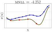
nargp
deep-mf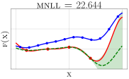
mf-dgp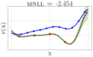

Figure 4: Cross-comparison across methods and synthetic examples for challenging multi-fidelity scenarios. mf-dgp yields conservative uncertainty estimates where few high-fidelity observations are available.

5 Experiments

In the preceding sections, we developed a multi-fidelity model that can be trained end-to-end across fidelities. Through a series of experiments, we validate that beyond its theoretic appeal, the proposed mf-dgp model also works well in practice. We begin with a visual illustration of the superior uncertainty quantification returned by the model, and corroborate these findings by comparing it against competing techniques on a suite of established multi-fidelity problems with varying fidelity levels. This is followed by an experiment involving a large-scale real-world dataset for which nearly a million observations are available. An experimental design set-up showcasing the benefits of using mf-dgp in conjunction with determinantal point processes concludes this section.

5.1 Synthetic Examples

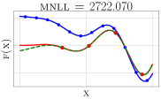
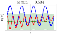
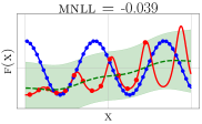
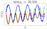
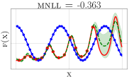
One of the primary motivations for undertaking this work was to develop a fully-fledged multi-fidelity model which avoids the overfitting issues encountered in existing models. We commence this section by considering experimental set-ups where the available data is generally insufficient to yield confident predictions, and higher uncertainty is prized. In particular, we consider four synthetic examples (plotted in Figure 3) - two where the correlation between fidelities is linear, and two where this is nonlinear. We train mf-dgp using the two-step procedure described in Section 4.5, whereby the noise variance and variational parameters are fixed for the first 5,000 training steps, before being trained jointly with the rest for another 15,000 steps. For increased stability, the variational distributions at lower fidelities are initially fixed to the known training targets; these are then freed and optimization is continued. The Adam optimizer (Kingma & Ba, 2015) is used with learning rate set to 0.003 and 0.001 for the first and second training phases respectively. Training generally converges in fewer iterations, but we keep this configuration for conformity.

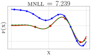
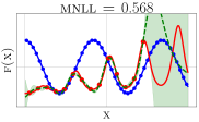
In Figure 4, we compare our model to ar1, nargp, and deep-mf on multi-fidelity scenarios where the allocation of high-fidelity data is either limited or constrained to one area of the input domain. In all examples, our model yields appropriately conservative estimates in regions where insufficient observations are available. The improved uncertainty quantification can be validated visually for these one-dimensional examples, but this is also corroborated by the superior mean negative log likelihood (mnll) reported for mf-dgp on the test data.

5.2 Benchmark Comparison

Table 1: Model Comparison on Multi-fidelity Benchmark Examples.

3		fidelity	ar1			nargp			mf-dgp
benchmark	$D_{\text{in}}$	allocation	r${}^{2}$	rmse	mnll	r${}^{2}$	rmse	mnll	r${}^{2}$	rmse	mnll
currin	2	12-5	0.913	0.677	20.105	0.903	0.740	20.817	0.935	0.601	0.763
park	4	30-5	0.985	0.575	465.377	0.954	0.928	743.119	0.985	0.565	1.383
borehole	8	60-5	1.000	0.005	-3.946	0.973	0.063	-1.054	0.999	0.015	-2.031
branin	2	80-30-10	0.891	0.044	-1.740	0.929	0.053	-1.223	0.965	0.030	-2.572
hartmann-3d	3	80-40-20	0.998	0.043	0.440	0.305	0.755	0.637	0.994	0.075	-0.731

true high-fidelity	predicted high-fidelity	dpp samples

Figure 5: Real-world experiment indicating the infection rate of Plasmodium falciparum among African children. Lighter-shaded regions denote higher infection rates in that area of the continent. Left: True infection rates recorded for the year 2015. Center: mf-dgp predictions given low-fidelity data from 2005 and limited high-fidelity training points (marked in red) from 2015. Right: White squares show the samples drawn from a dpp using the posterior covariance of the mf-dgp model as its kernel.

Beyond the synthetically-constructed examples considered thus far, we verify the suitability of using mf-dgp over existing methods by benchmarking their performance on a selection of well-known multi-fidelity problems (full specification in the supplementary material). Five randomly-generated datasets are prepared for each example function, following the allocation of points to different fidelities listed in Table 1. The results denote the R-squared $(\textsc{R}^{2})$, root mean squared error (rmse), and mnll obtained using each model over a fixed test set of 1,000 points covering the entire input domain. The obtained results give credence to our intuition that mf-dgp balances issues in alternative modeling approaches, which are singularly tailored for linear and nonlinear fidelity correlations respectively. Notably, for the 3-level Branin function having nonlinear correlations between fidelities, the ar1 model is incapable of properly modeling the high-fidelity data, whereas mf-dgp significantly outperforms nargp on all metrics.

5.3 Large-scale Real-world Experiment

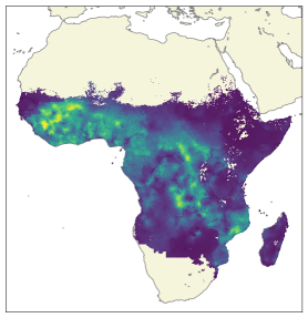
We now proceed to demonstrate the effectiveness of mf-dgp on a real-world dataset which also shows how mini-batch-based training with svi is essential for modeling large datasets beyond the scale to which multi-fidelity methods are usually applied. In particular, we fit mf-dgp to data describing the infection rate of Plasmodium falciparum (a known cause of malaria) among children in Africa, illustrated in Figure 5 (left). For our evaluation, we treat data from 2005 as being low-fidelity and more recent data from 2015 as high-fidelity; this permits us to exploit ample historical data to build an accurate model of the current infection rate for which fewer observations are given. As the targets lie on the interval $[0,1]$, we transform these using a logit function before fitting the model.

We train the model with 800,000 low-fidelity data-points and 1,000 high-fidelity observations, where each mini-batch consists of 1,000 low-fidelity and all 1,000 high-fidelity points. Optimization is carried out using Adam for 30,000 iterations, while 1,000 inducing points are used at each layer. Upon training, the model was evaluated on a test set comprising of 10,000 high-fidelity points. The results obtained by mf-dgp on this data are visualized in Figure 5 (center), with an rmse of 0.063. In contrast, an exact gp trained only on high-fidelity observations scores an inferior rmse of 0.096.

5.4 Experimental Design with mf-dgp

Lastly, we demonstrate how the posterior distribution associated with our mf-dgp model can be used for the purpose of experimental design. In particular, we validate how this can be exploited in order to make decisions on where to obtain new observations of infection rates such that the overall quality of predictions returned by the model is improved. We are generally interested in observing these new points with high-fidelity at locations where either uncertainty is large (leading to a more diverse set of locations) or where we expect there to be a substantial infection rate (denoted by lighter shading on the map). This balances the exploration-exploitation trade-off that is commonly targeted by such schemes.

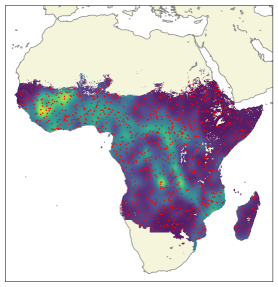
A determinantal point process (dpp; Macchi, 1975) is well-suited for addressing the aforementioned criteria; the kernel function of a dpp is chosen to be $\mu(\mathbf{x})k(\mathbf{x},\mathbf{x}^{\prime})\mu(\mathbf{x}^{\prime})$, where $k(\cdot,\cdot)$ and $\mu(\cdot)$ denote the posterior covariance and mean functions of the mf-dgp model. The covariance term encourages points to be selected at a set of diverse locations where the model uncertainty is high, whereas the mean term gives greater weight to input locations where the infection rate is expected to be high. In order to sample from the dpp, we first evaluate the mean and covariance of the trained mf-dgp at a randomly-selected set of 2,500 input locations. By setting the cardinality $k=50$, a $k$-dpp (Kulesza & Taskar, 2011) is then used to sample 50 high-fidelity points from this subset, which are then interpreted as the locations at which true infection rates should be acquired. Extending the experiment presented in the previous section, the sampled points are illustrated by white markers in Figure 5 (right). Recalling the criteria highlighted at the beginning of this section, the plot clearly indicates that the points selected by this procedure are adequately dispersed across the map, with increased concentration in areas where infection rates are predicted to be high. This validates the suitability of our multi-fidelity model in a pipelined decision-making scheme.

6 Conclusion

Reliable decision making under uncertainty is a core requirement in multi-fidelity scenarios where unbiased observations are scarce or difficult to obtain. In this paper, we proposed the first complete specification of a multi-fidelity model as a dgp that is capable of capturing nonlinear relationships between fidelities with reduced overfitting. By providing end-to-end training across all fidelity levels, mf-dgp consistently yields superior quantification and propagation of uncertainty that is crucial in active learning and iterative methods such as experimental design. The application of state-of-the-art dgps to an unconventional setting is also essential for broadening their appeal to a wider community of researchers and practitioners alike.

Effectively optimizing the inducing variables at each layer while remaining faithful to the implicit multi-fidelity constraints is a challenging problem which warrants further investigation, and is key to extending the learning capacity of mf-dgp. On another note, in contrast to the standard ar1 model, the compositional structure of mf-dgp hinders the specification of analytic expressions for the acquisition functions prevalent in procedures such as Bayesian optimization or quadrature. Beyond the multi-fidelity setting explored here, the latter requirement accentuates ongoing effort to develop active learning schemes that are better-suited for deep models.

Deep Gaussian Processes for Multi-fidelity Modeling

Appendix A Further Model Details

For completeness, in the following appendix we extend the model description given in Section 4 of the main paper. In particular, we detail the variational approximation for the model and derive the evidence lower bound that serves the role of our model’s multi-fidelity objective function with respect to which parameters are optimized. As in the main text, we intentionally remain faithful to the general notation and structure of Salimbeni & Deisenroth (2017) in order to place emphasis on the multi-fidelity extension being proposed in this work as opposed to the dgp approximation upon which it is based.

A.1 Approximating the Marginal Likelihood of mf-dgp

Assume that each layer, $l$, of our mf-dgp model corresponds to a realisation of the process modeled with fidelity $t$. For a dataset with $T$ fidelities, the marginal likelihood of our mf-dgp model is then given by:

$$\mathcal{L_{\textsc{mf-dgp}}}=\mathbb{E}_{q\left(\{\{\mathbf{f}_{l}^{t}\}^{t}_{l=1}\}_{t=1}^{T},\{\mathbf{u}_{l}\}^{L}_{l=1}\right)}\left[\log\left(\frac{p\left(\{\textbf{y}^{t},\{\mathbf{f}_{l}^{t}\}_{l=1}^{t}\}_{t=1}^{T},\{\mathbf{u}_{l}\}^{L}_{l=1}\right)}{q\left(\{\{\mathbf{f}_{l}^{t}\}^{t}_{l=1}\}_{t=1}^{T},\{\mathbf{u}_{l}\}^{L}_{l=1}\right)}\right)\right].$$ (12)

We have that:

$$p\left(\{\mathbf{y}^{t},\{\mathbf{f}_{l}^{t}\}_{l=1}^{t}\}_{t=1}^{T},\{\mathbf{u}_{l}\}^{L}_{l=1}\right)= \prod_{t=1}^{T}\prod^{N_{t}}_{i=1}p\left({y}^{i,t}|{f}^{i,t}_{t}\right)\prod_{l=1}^{t}p\left(\mathbf{f}^{t}_{l}|\mathbf{u}_{l};\{\mathbf{f}^{t}_{l-1},\textbf{X}^{t}\},\textbf{Z}_{l-1}\right)\times$$

$$\prod_{l=1}^{L}p\left(\mathbf{u}_{l};\mathbf{Z}_{l-1}\right),$$ (13)

where $N_{t}$ denotes the number of data points observed with fidelity level $t$. Similarly the denominator in the expectation can be expanded as:

$$q\left(\{\{\mathbf{f}_{l}^{t}\}^{t}_{l=1}\}_{t=1}^{T},\{\mathbf{u}_{l}\}^{L}_{l=1}\right)= \prod_{t=1}^{T}\prod_{l=1}^{t}p\left(\mathbf{f}_{l}^{t}|\mathbf{u}_{l};\{\mathbf{f}^{t}_{l-1},\textbf{X}^{t}\},\mathbf{Z}_{l-1}\right)\times$$

$$\prod_{l=1}^{L}q\left(\mathbf{u}_{l}\right).$$ (14)

By inserting Equations (A.1) and (A.1) in (12), and canceling out equivalent terms in the numerator and denominator, we obtain the following variational lower bound on the marginal likelihood of our multi-fidelity model:

$$\mathcal{L_{\textsc{mf-dgp}}} =\iint q\left(\{\{\mathbf{f}_{l}^{t}\}^{t}_{l=1}\}_{t=1}^{T},\{\mathbf{u}_{l}\}^{L}_{l=1}\right)\log\left(\frac{\prod_{t=1}^{T}\prod^{N_{t}}_{i=1}p\left({y}^{i,t}|{f}^{i,t}_{t}\right)\times\prod_{l=1}^{L}p\left(\mathbf{u}_{l};\mathbf{Z}_{l-1}\right)}{\prod_{l=1}^{L}q\left(\mathbf{u}_{l}\right)}\right)$$

$$\quad\text{d}\{\{\mathbf{f}_{l}^{t}\}^{t}_{l=1}\}_{t=1}^{T},\{\mathbf{u}_{l}\}^{L}_{l=1}$$

$$=\iint q\left(\{\{\mathbf{f}_{l}^{t}\}^{t}_{l=1}\}_{t=1}^{T},\{\mathbf{u}_{l}\}^{L}_{l=1}\right)\log\left(\prod_{t=1}^{T}\prod^{N_{t}}_{i=1}p\left({y}^{i,t}|{f}^{i,t}_{t}\right)\right)\text{d}\{\{\mathbf{f}_{l}^{t}\}^{t}_{l=1}\}_{t=1}^{T},\{\mathbf{u}_{l}\}^{L}_{l=1}$$

$$\quad+\iint q\left(\{\{\mathbf{f}_{l}^{t}\}^{t}_{l=1}\}_{t=1}^{T},\{\mathbf{u}_{l}\}^{L}_{l=1}\right)\log\left(\frac{\prod_{l=1}^{L}p\left(\mathbf{u}_{l};\mathbf{Z}_{l-1}\right)}{\prod_{l=1}^{L}q\left(\mathbf{u}_{l}\right)}\right)\text{d}\{\{\mathbf{f}_{l}^{t}\}^{t}_{l=1}\}_{t=1}^{T},\{\mathbf{u}_{l}\}^{L}_{l=1}$$

$$=\int q\left(\{\{\mathbf{f}_{l}^{t}\}^{t}_{l=1}\}_{t=1}^{T}\right)\log\left(\prod_{t=1}^{T}\prod^{N_{t}}_{i=1}p\left({y}^{i,t}|{f}^{i,t}_{t}\right)\right)\text{d}\{\{\mathbf{f}_{l}^{t}\}^{t}_{l=1}\}_{t=1}^{T}$$

$$\quad+\int q\left(\{\mathbf{u}_{l}\}^{L}_{l=1}\right)\log\left(\frac{\prod_{l=1}^{L}p\left(\mathbf{u}_{l};\mathbf{Z}_{l-1}\right)}{\prod_{l=1}^{L}q\left(\mathbf{u}_{l}\right)}\right)\text{d}\{\mathbf{u}_{l}\}^{L}_{l=1}$$

$$=\sum_{t=1}^{T}\int q\left(\{\mathbf{f}_{l}^{t}\}^{t}_{l=1}\right)\log\left(\prod_{i=1}^{N_{t}}p\left({y}^{i,t}|{f}^{i,t}_{t}\right)\right)\text{d}\{\mathbf{f}_{l}^{t}\}^{t}_{l=1}$$

$$\quad+\sum_{l=1}^{L}D_{\text{KL}}\left[q\left(\mathbf{u}_{l}\right)||\;p\left(\mathbf{u}_{l};\mathbf{Z}_{l-1}\right)\right]$$

$$=\sum_{t=1}^{T}\sum_{i=1}^{N_{t}}\mathbb{E}_{q\left({f}^{i,t}_{t}\right)}\left[\log p\left({y}^{i,t}|{f}^{i,t}_{t}\right)\right]$$

$$\quad+\sum_{l=1}^{L}D_{\text{KL}}\left[q\left(\mathbf{u}_{l}\right)||\;p\left(\mathbf{u}_{l};\mathbf{Z}_{l-1}\right)\right].$$ (15)

If both the true distribution and the variational approximation are assumed to be Gaussian, the $D_{\text{KL}}$ term can conveniently be evaluated analytically.

A.2 Reparameterization Trick

As with other dgp models (Dai et al., 2016; Cutajar et al., 2017) trained using stochastic variational inference (see Section 4.5), the reparameterization trick (Kingma & Welling, 2014) is then used to recursively draw samples from the variational posterior:

$${\hat{f}}^{i,t}_{l}= \;\widetilde{\mathbf{m}}_{l}\left(\left\{{\hat{f}}^{i,t}_{l-1},\textbf{x}^{i,t}\right\}\right)+$$

$$\;\mathbf{\varepsilon}^{i,t}_{l}\odot\sqrt{\widetilde{\mathbf{S}}_{l}\left(\left\{{\hat{f}}^{i,t}_{l-1},\textbf{x}^{i,t}\right\},\left\{{\hat{f}}^{i,t}_{l-1},\textbf{x}^{i,t}\right\}\right)}\;\;,$$ (16)

where $\mathbf{\varepsilon}^{i,t}_{l}\sim\mathcal{N}\left(\textbf{0},\textbf{I}_{D_{\text{out}}}\right)$.

Appendix B Additional Detail on Experiments

This appendix contains further information on the experimental evaluation provided in Section 5 of the main paper which was excluded due to space constraints.

B.1 Mapping Between Fidelities for Synthetic Examples

Table 2: Detail of synthetically-constructed functions used in experimental evaluation.

3 example	fidelity	function
linear-a	low	$y_{l}\left(x\right)=\frac{1}{2}y_{h}\left(x\right)+10\left(x-\frac{1}{2}\right)+5$
	high	$y_{h}\left(x\right)=\left(6x-2\right)^{2}\sin\left(12x-4\right)$
linear-b	low	$y_{l}\left(x\right)=2y_{h}\left(x\right)+\left(x^{3}-\frac{1}{2}\right)\sin\left(3x-\frac{1}{2}\right)+4\cos\left(2x\right)$
	high	$y_{h}(x)=5x^{2}\sin(12x)$
nonlinear-a	low	$y_{l}\left(x\right)=\sin\left(8\pi x\right)$
	high	$y_{h}\left(x\right)=\left(x-\sqrt{2}\right)\left(y_{l}\left(x\right)\right)^{2}$
nonlinear-b	low	$y_{l}\left(x\right)=\cos\left(15x\right)$
	high	$y_{h}\left(x\right)=xe^{y_{l}\left(2x-.2\right)}-1$

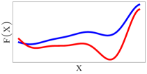
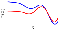
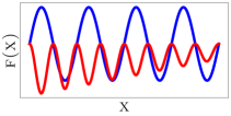
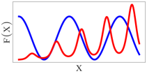
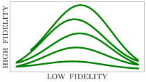
In the first experiment presented in Section 5, we evaluated the performance of our model on four example functions, two having a linear mapping between fidelities and another two with nonlinear mappings; their precise definition is given in Table 2. The relationships between fidelities for these example functions are illustrated in Figure 6, where the bottom row shows the mapping from low-fidelity observations to their high-fidelity counterparts. It is difficult to infer much useful information about the problem from simply observing these plots; however, the additional complexity of the two nonlinear examples is indicative of where the standard ar1 model can be expected to perform badly.

linear-a	linear-b

(a) Linear mapping.

nonlinear-a	nonlinear-b

(b) Nonlinear mapping.

Figure 6: Top: Synthetic multi-fidelity functions used for model comparison. Bottom: Mapping between low and high-fidelity observations for same functions.

In our evaluation, we observed that all methods worked best when the output values for all fidelities were scaled down, particularly for ensuring convergence in the optimization procedure. To this end, in the experiments we scale down the original functions by a constant scaling factor while still preserving the relationship between fidelities in their original formulation.

B.2 Specification of Benchmark Problems

In Section 5.2 of the main paper, we evaluated the performance of our model on a set of five benchmark problems that are widely used in the literature for evaluating the effectiveness of multi-fidelity methods. The specification of each problem is given below:

• currin

  The currin function is a two-dimensional problem that is commonly featured in works related to simulating computer experiments, with input domain $\mathbf{x}\in\left[0,1\right]^{2}$. The high-fidelity variation of this function is given by:

  $$y_{h}\left(\mathbf{x}\right)=\left[1-\exp\left(-\frac{1}{2x_{2}}\right)\right]\frac{2300x_{1}^{3}+1900x_{1}^{2}+2092x_{1}+60}{100x_{1}^{3}+500x_{1}^{2}+4x_{1}+20}\text{,}$$

  whereas the low-fidelity alternative is given by:

  $$y_{l}\left(\mathbf{x}\right)= \frac{1}{4}\left[y_{h}\left(x_{1}+0.05,x_{2}+0.05\right)+y_{h}\left(x_{1}+0.05,\max\left(0,x_{2}-0.05\right)\right)\right]+$$

  $$\frac{1}{4}\left[y_{h}\left(x_{1}-0.05,x_{2}+0.05\right)+y_{h}\left(x_{1}-0.05,\max\left(0,x_{2}-0.05\right)\right)\right]\text{;}$$

• park

  The park function is a four-dimensional problem where all inputs lie in the range $\left[0,1\right]$. High-fidelity observations are evaluated as:

  $$y_{h}\left(\mathbf{x}\right)=\frac{x_{1}}{2}\left[\sqrt{1+\left(x_{2}+x_{3}^{2}\right)\frac{x_{4}}{x_{1}^{2}}}-1\right]+\left(x_{1}+3x_{4}\right)\exp\left[1+\sin\left(x_{3}\right)\right]\text{,}$$

  while low-fidelity observations are obtained using:

  $$y_{l}\left(\mathbf{x}\right)=\left[1+\frac{\sin\left(x_{1}\right)}{10}\right]y_{h}\left(\mathbf{x}\right)-2x_{1}+x_{2}^{2}+x_{3}^{2}+0.5\text{;}$$

• borehole

  The borehole example is a two-level physical model that simulates water flow through a borehole, and depends on eight input parameters. The input domain is constrained to lie in the following regions: $x_{1}\in\left[0.05,0.15\right]$, $x_{2}\in\left[100,50000\right]$, $x_{3}\in\left[63070,115600\right]$, $x_{4}\in\left[990,1110\right]$, $x_{5}\in\left[63.1,115\right]$, $x_{6}\in\left[700,820\right]$, $x_{7}\in\left[1120,1680\right]$, $x_{8}\in\left[9855,12045\right]$. The high-fidelity simulation for this model is given by:

  $$y_{h}\left(\mathbf{x}\right)=\frac{2\pi x_{3}\left(x_{4}-x_{6}\right)}{\log\left(x_{2}/x_{1}\right)\left(1+\frac{2x_{7}x_{3}}{\log\left(x_{2}/x_{1}\right)x_{1}^{2}x_{8}}\right)+\frac{x_{3}}{x_{5}}}\text{,}$$

  while the low-fidelity variant is evaluated as:

  $$y_{l}\left(\mathbf{x}\right)=\frac{5x_{3}\left(x_{4}-x_{6}\right)}{\log\left(x_{2}/x_{1}\right)\left(1.5+\frac{2x_{7}x_{3}}{\log\left(x_{2}/x_{1}\right)x_{1}^{2}x_{8}}\right)+\frac{x_{3}}{x_{5}}}\text{;}$$

• branin

  The three-level branin function is taken from the specification given in Perdikaris et al. (2017), where the two-dimensional input lies in the range $\left[-5,10\right]\times\left[0,15\right]$. The three tiers are given by:

  $$y_{h}\left(\mathbf{x}\right)=\left(\frac{-1.275x_{1}^{2}}{\pi^{2}}+\frac{5x_{1}}{\pi}+x_{2}-6\right)^{2}+\left(10-\frac{5}{4\pi}\right)\cos\left(x_{1}\right)+10\text{,}$$

  $$y_{m}\left(\mathbf{x}\right)=10\sqrt{y_{h}\left(\mathbf{x}-2\right)}+2\left(x_{1}-0.5\right)-3\left(3x_{2}-1\right)-1\text{, and}$$

  $$y_{l}\left(\mathbf{x}\right)=y_{m}\left(1.2\left(\mathbf{x}+2\right)\right)-3x_{2}+1\text{;}$$

• hartmann-3d

  Finally, the three-level hartmann-3d example follows the specification provided in Kandasamy et al. (2016), whereby the three-dimensional input lies in the domain $\left[0,1\right]^{3}$. The evaluation of observations with fidelity $t$ is given by:

  $$y_{t}\left(\mathbf{x}\right)=\sum_{i=1}^{4}\alpha_{i}\exp\left(-\sum_{j=1}^{3}A_{ij}\left(x_{j}-P_{ij}\right)^{2}\right)\text{,}$$

  where

  A = [3 10 30 0.1 10 35 3 10 30 0.1 10 35 ]   and  P = [0.3689 0.1170 0.2673 0.4699 0.4387 0.7470 0.1091 0.8732 0.5547 0.0381 0.5743 0.8828 ] .

  The vector $\boldsymbol{\alpha}$ is initially set to $\left[1.0,1.2,3.0,3.2\right]^{\top}$ and is updated to $\boldsymbol{\alpha}_{t}=\boldsymbol{\alpha}+(3-t)\boldsymbol{\delta}$ for lower fidelities, where $\boldsymbol{\delta}=\left[0.01,-0.01,-0.1,0.1\right]^{\top}$.

B.3 Configuration of Competing Models

In this final section, we elaborate on the configuration and optimization strategies used for the competing techniques in Section 5 of the paper.

• ar1 (Kennedy & O’Hagan, 2000)

  The ar1 model is implemented as per the original specification presented by Kennedy & O’Hagan (2000). We opt for this formulation instead of the procedure detailed in Le Gratiet & Garnier (2014) since the latter is more cumbersome to adapt to non-nested input structures, whereas this constraint does not apply to the former. We assign independent noise parameters to each fidelity, which are jointly optimized with the kernel hyperparameters and scaling factors in a single call to the optimization procedure.

• nargp (Perdikaris et al., 2017)

  For the nargp model, we adopt the same optimization strategy considered by Perdikaris et al. (2017) in their evaluation. In particular, individual gps are used for modeling the data at each fidelity level, and these are optimized sequentially in isolation. We optimize the kernel parameters for the gps at each layer using a two-step procedure which was applied in the original implementation provided by the authors - the optimization is first carried out with fixed noise variance, after which this parameter is also freed and all parameters are adapted jointly.

• deep-mf (Raissi & Karniadakis, 2016)

  One of the challenges associated with the deep-mf model is in selecting an appropriate deterministic nonlinear transformation to be applied to the input data. Given that there is no straightforward approach for deciding how to configure this component of the model, in our evaluation we use the two-layer neural network with sigmoid activation functions reported in the original presentation of the model given by Raissi & Karniadakis (2016). The process noise is shared between fidelities. No pre-existing code was found for this model.

References

- Calandra et al. (2016) Calandra, R., Peters, J., Rasmussen, C. E., and Deisenroth, M. P. Manifold Gaussian processes for regression. In International Joint Conference on Neural Networks (IJCNN), pp. 3338–3345, 2016.
- Cutajar et al. (2017) Cutajar, K., Bonilla, E. V., Michiardi, P., and Filippone, M. Random feature expansions for deep Gaussian processes. In 34th International Conference on Machine Learning (ICML), pp. 884–893, 2017.
- Cutler et al. (2014) Cutler, M., Walsh, T. J., and How, J. P. Reinforcement learning with multi-fidelity simulators. In 2014 IEEE International Conference on Robotics and Automation (ICRA), pp. 3888–3895, 2014.
- Dai et al. (2016) Dai, Z., Damianou, A., González, J., and Lawrence, N. Variational auto-encoded deep Gaussian processes. In 4th International Conference on Learning Representations (ICLR), 2016.
- Damianou (2015) Damianou, A. Deep Gaussian processes and variational propagation of uncertainty. PhD thesis, University of Sheffield, 2015.
- Damianou & Lawrence (2013) Damianou, A. and Lawrence, N. D. Deep Gaussian processes. In 16th International Conference on Artificial Intelligence and Statistics (AISTATS), pp. 207–215, 2013.
- Duvenaud et al. (2014) Duvenaud, D. K., Rippel, O., Adams, R. P., and Ghahramani, Z. Avoiding pathologies in very deep networks. In 17th International Conference on Artificial Intelligence and Statistics (AISTATS), pp. 202–210, 2014.
- Hensman et al. (2013) Hensman, J., Fusi, N., and Lawrence, N. D. Gaussian processes for big data. In 29th Conference on Uncertainty in Artificial Intelligence (UAI), 2013.
- Hoffman et al. (2013) Hoffman, M. D., Blei, D. M., Wang, C., and Paisley, J. W. Stochastic variational inference. Journal of Machine Learning Research, 14(1):1303–1347, 2013.
- Kandasamy et al. (2016) Kandasamy, K., Dasarathy, G., Póczos, B., and Schneider, J. G. The multi-fidelity multi-armed bandit. In Advances in Neural Information Processing Systems 29 (NeurIPS), pp. 1777–1785, 2016.
- Kennedy & O’Hagan (2000) Kennedy, M. C. and O’Hagan, A. Predicting the output from a complex computer code when fast approximations are available. Biometrika, 87(1):1–13, 2000.
- Kingma & Ba (2015) Kingma, D. P. and Ba, J. Adam: A method for stochastic optimization. In 3rd International Conference on Learning Representations (ICLR), 2015.
- Kingma & Welling (2014) Kingma, D. P. and Welling, M. Auto-encoding variational Bayes. In 2nd International Conference on Learning Representations (ICLR), 2014.
- Koziel & Leifsson (2013) Koziel, S. and Leifsson, L. Multi-level CFD-based airfoil shape optimization with automated low-fidelity model selection. In ICCS, volume 18 of Procedia Computer Science, pp. 889–898. Elsevier, 2013.
- Kulesza & Taskar (2011) Kulesza, A. and Taskar, B. k-DPPs: Fixed-size determinantal point processes. In 28th International Conference on Machine Learning (ICML), pp. 1193–1200, 2011.
- Lam et al. (2015) Lam, R., Allaire, D. L., and Willcox, K. E. Multifidelity optimization using statistical surrogate modeling for non-hierarchical information sources. In 56th AIAA/ASCE/AHS/ASC Structures, Structural Dynamics, and Materials Conference. American Institute of Aeronautics and Astronautics, 2015.
- Le Gratiet & Garnier (2014) Le Gratiet, L. and Garnier, J. Recursive co-kriging model for design of computer experiments with multiple levels of fidelity. International Journal for Uncertainty Quantification, 4(5), 2014.
- Liu et al. (2018) Liu, H., Ong, Y., Cai, J., and Wang, Y. Cope with diverse data structures in multi-fidelity modeling: A Gaussian process method. Eng. Appl. of AI, 67:211–225, 2018.
- Macchi (1975) Macchi, O. The coincidence approach to stochastic point processes. Advances in Applied Probability, 7:83–122, 1975.
- MacKay (2003) MacKay, D. J. Information theory, inference and learning algorithms, chapter 28, pp. 343–355. Cambridge university press, 2003.
- Majda & Gershgorin (2010) Majda, A. J. and Gershgorin, B. Quantifying uncertainty in climate change science through empirical information theory. Proceedings of the National Academy of Sciences, 107(34):14958–14963, 2010.
- Matthews et al. (2017) Matthews, A. G. d. G., van der Wilk, M., Nickson, T., Fujii, K., Boukouvalas, A., León-Villagrá, P., Ghahramani, Z., and Hensman, J. GPflow: A Gaussian process library using TensorFlow. Journal of Machine Learning Research, 18:40:1–40:6, 2017.
- Morris (2004) Morris, M. D. The design and analysis of computer experiments. Journal of the American Statistical Association, 99(468):1203–1204, 2004.
- Peherstorfer et al. (2018) Peherstorfer, B., Willcox, K., and Gunzburger, M. Survey of multifidelity methods in uncertainty propagation, inference, and optimization. SIAM Review, 60(3):550–591, 2018.
- Perdikaris et al. (2017) Perdikaris, P., Raissi, M., Damianou, A., Lawrence, N. D., and Karniadakis, G. E. Nonlinear information fusion algorithms for data-efficient multi-fidelity modelling. Proc. R. Soc. A, 473(2198):20160751, 2017.
- Poloczek et al. (2017) Poloczek, M., Wang, J., and Frazier, P. I. Multi-information source optimization. In Advances in Neural Information Processing Systems 30 (NeurIPS), pp. 4291–4301, 2017.
- Raissi & Karniadakis (2016) Raissi, M. and Karniadakis, G. Deep multi-fidelity Gaussian processes. arXiv preprint arXiv:1604.07484, 2016.
- Rasmussen & Williams (2006) Rasmussen, C. E. and Williams, C. Gaussian Processes for Machine Learning. MIT Press, 2006.
- Requeima et al. (2019) Requeima, J., Tebbutt, W., Bruinsma, W., and Turner, R. E. The Gaussian process autoregressive regression model (GPAR). In 22nd International Conference on Artificial Intelligence and Statistics (AISTATS), 2019.
- Salimbeni & Deisenroth (2017) Salimbeni, H. and Deisenroth, M. P. Doubly stochastic variational inference for deep Gaussian processes. In Advances in Neural Information Processing Systems 30 (NeurIPS), pp. 4591–4602, 2017.
- Sen et al. (2018) Sen, R., Kandasamy, K., and Shakkottai, S. Multi-fidelity black-box optimization with hierarchical partitions. In 35th International Conference on Machine Learning (ICML), pp. 4545–4554, 2018.
- Shahriari et al. (2016) Shahriari, B., Swersky, K., Wang, Z., Adams, R. P., and de Freitas, N. Taking the human out of the loop: A review of Bayesian optimization. Proceedings of the IEEE, 104(1):148–175, 2016.
- Ulaganathan et al. (2016) Ulaganathan, S., Couckuyt, I., Dhaene, T., Degroote, J., and Laermans, E. Performance study of gradient-enhanced kriging. Engineering with Computers, 32(1):15–34, 2016.
- Zaytsev & Burnaev (2017) Zaytsev, A. and Burnaev, E. Large scale variable fidelity surrogate modeling. Ann. Math. Artif. Intell., 81(1-2):167–186, 2017.