Analytically computable symmetric quantum correlations

Abstract

One of the greatest challenges in developing the resource theory of a quantum feature is to establish an analytically computable quantifier, which directly limits the practicability of such quantifiers. Here, analytic quantifiers of both the symmetric quantum discord (SQD) and the symmetric measurement-induced nonlocality (SMIN) in a bipartite system of qubits are studied on the basis of the quantum skew information. It is shown that the SMIN of any two-qubit system and the SQD of bipartite ”X”-type states and block-diagonal states can be analytically determined. In addition, the SQD and the SMIN are invariant with an attached quantum state. The validity of our analytical expressions is further illustrated numerically on the basis of several randomly generated density matrices.

I Introduction

Quantum mechanical features are not only a fundamental aspect that distinguishes the quantum from the classical world but also an important physical resource for quantum information processing tasks (QIPTs). In recent years, the resource theory of quantum features has been attracting increasing interest (H1 ; H2 ; H3 and references therein); however, only limited progress has been made toward the most essential goal, i.e., the development of a good quantifier for a general quantum system. Quantum entanglement is the most remarkable example; for this quantum feature, the analytical quantifiers for a general quantum state are still restricted to those for bipartite pure states B1 ; B2 and mixed states in six dimensions (concurrence for qubit-qubit statese1 and negativity for qubit-qutrit states N1 ; Horo ; N2 ), which were well established approximately two decades ago. Needless to say, multipartite quantum states include many inequivalent classes of entanglement ee3 ; miy , and the quantification of a bipartite high-dimensional state is usually related to some complex optimization; consequently, it is difficult to formulate an analytical or even an economic and effective numerical way to quantify the entanglement of a general state. Therefore, the most fruitful approach is to focus on effective quantification only for states in certain specific classes CKW ; book ; adp ; G3 ; b1 ; b2 ; G4 ; ycc ; Ost ; Y3 ; ee2 ; ee4 . In addition, as a quantum correlation that extends beyond entanglement, the quantum discord (QD) d1 ; d2 , which quantifies the discrepancy between the quantum versions of two classically equivalent pieces of mutual information, can only be analytically calculated for a general state in $2\otimes n$ dimensions NS ; yzyz ; L1 ; SY ; RM ; OUT ; VON ; QUAN ; MULT ; EXPE ; QUANTU ; X1 ; X2 ; X3 . The same is true for its counterpart quantity loca ; Wu ; iajd , that is, the measurement-induced nonlocality (MIN) which characterizes the global disturbance in a composite state caused by a local nondisturbing measurement on one subsystem loca . Recently, some progress has been made in regard to analytical expressions for certain classes of states or effective numerical methods iajd ; L2 ; G1 ; KM ; yb ; S1 ; Hu ; JOIN . However, neither the QD nor the MIN of a bipartite system is symmetric in the sense that different results will be obtained (especially for some zero-discord states) if the two subsystems are swapped, which implies that the QD and MIN cannot completely quantify all of the quantum correlations present in a state. To overcome this shortcoming, symmetric versions of the QD and the MIN are defined, i.e., the symmetric quantum discord (SQD) Di1 ; Di2 ; Di3 and the symmetric measurement-induced nonlocality (SMIN). In particular, with the development of the resource theory of quantum coherence Y1 ; QQ1 ; c1 ; c2 ; c3 ; c4 ; c5 ; c6 ; c7 ; c8 ; c9 ; c10 ; QQ3 ; QQ2 ; M1 ; zhou ; QUANTI ; ACCE , it was shown that the coherence of a system could be converted through incoherent operations into the SQD, instead of the asymmetric QD, of a composite system QQ1 ; QQ2 ; QQ3 . By considering different bases, the coherence can also be related to the SMIN. This finding suggests that these symmetric quantum correlations could have fundamental meaning and potentially useful applications. Outside of the context of the resource theory mentioned above, much less progress has been made with regard to symmetric quantum correlations, although it has been shown that the geometric SQDs of some types of systems can be analytically calculated Di2 . However, the geometric SQD seems not to be a good measure because forming a composite state by taking the product with another mixed state will reduce the SQD of the state of interest M1 .

In this paper, we study the analytical expressions for the SQD and SMIN of a bipartite system of qubits. We define the SQD and SMIN in terms of the quantum skew information skew ; skew1 ; skew2 ; skew3 with regard to the state of interest and projective measurements. It is obvious that neither the SQD nor the SMIN will change if we take the product of another state with the considered state based on the quantum skew information. Most importantly, we find the analytical expression for the SMIN of any bipartite state of qubits and find that the SQD can be analytically calculated for any bipartite ”X”-type states and block-diagonal states. As application examples, we calculate both the SQD and the SMIN for several randomly generated states. The numerical results are completely consistent with our analytical expressions. The remainder of this paper is organized as follows. In Sec. II, we introduce the definitions of the SQD and SMIN based on the quantum skew information. In Sec. III, we present the analytical expressions for both the SQD and SMIN as our main theorems. In Sec. IV, we consider several randomly generated examples to test our analytical expressions. Sec. V presents a discussion of our results and our conclusions.

II Definitions of the SQD and SMIN based on the skew information

Before presenting the definitions of both the SQD and the SMIN, we would like to introduce the definitions of the QD and MIN which will be given based on the $l_{2}$ norm for the sake of intuitive understanding despite the noncontractive nature of the $l_{2}$ norm. For a bipartite density matrix $\rho_{AB}$, the (geometric) QD is defined as the minimal distance away from the state that is disturbed by local projective measurements NS as follows:

$$\tilde{D}\left(\rho_{AB}\right)=\min_{\Pi^{A}}\left\|\rho-\Pi^{A}(\rho_{AB})\right\|_{2}^{2},$$ (1)

where $\left\{\Pi^{A}\right\}$, defined as $\sum_{k}(\Pi_{k}^{A}\otimes I^{B})\rho_{AB}(\Pi_{k}^{A}\otimes I^{B})$, denotes the projective measurements on subsystem A and $\left\|\cdot\right\|_{2}$ denotes the $l_{2}$ norm of a matrix. Similarly, the MIN is defined as the maximal distance away from the state that is disturbed by local and subsystem-immune projective measurements loca as follows:

$$\tilde{N}(\rho_{AB})=\max_{\Pi^{\prime A}}\left\|\rho-\Pi^{\prime A}(\rho_{AB})\right\|_{2}^{2},$$ (2)

where $\left\{\Pi^{\prime A}\right\}$ is defined similarly to $\left\{\Pi^{A}\right\}$ but requires $\sum_{k}\Pi_{k}^{\prime A}\rho_{A}\Pi_{k}^{\prime A}=\rho_{A}$ to guarantee that the reduced density matrix $\rho_{A}=\mathrm{Tr}_{B}\rho_{AB}$ is not disturbed. It is apparent that the QD and MIN are not symmetric since the projective measurements are performed on only one subsystem. The two definitions above have a common drawback, namely, they will changed if we take the product of an additional mixed state with the state of interest; this change is directly induced by the properties of the $l_{2}$ norm. This drawback would naturally be inherited if we were to define the SQD and SMIN based on the $l_{2}$ norm. Therefore, in what follows, we will present our definitions of the SQD and SMIN in terms of the quantum skew information.

Definition 1.- For a bipartite $\left(m\otimes n\right)$-dimensional quantum state $\rho_{AB}$, the symmetric quantum discord (SQD) based on the skew information is defined as

$$D(\rho_{AB})=\min_{\left\{\left|k_{A}\right\rangle\right\},\left\{\left|k_{B}\right\rangle\right\}}\sum_{k_{A}=0}^{m-1}\sum_{k_{B}=0}^{n-1}I(\rho_{AB},K_{k_{A}k_{B}}),$$ (3)

where

$$I(\rho_{AB},K_{k_{A}k_{B}})=-\frac{1}{2}\mathrm{Tr}[\sqrt{\rho_{AB}},K_{k_{A}k_{B}}]^{2}$$ (4)

$$= \left\langle k_{A}k_{B}\right|\rho_{AB}\left|k_{A}k_{B}\right\rangle-\left|\left\langle k_{A}k_{B}\right|\sqrt{\rho_{AB}}\left|k_{A}k_{B}\right\rangle\right|^{2}$$

is the quantum skew information and $K_{k_{A}k_{B}}=\left|k_{A}\right\rangle_{A}\left\langle k_{A}\right|\otimes$ $\left|k_{B}\right\rangle_{B}\left\langle k_{B}\right|$ denotes the projective measurements on both subsystems.

Definition 2.-The symmetric measurement-induced nonlocality (SMIN) based on the skew information of the above quantum state $\rho_{AB}$, is defined as

$$N(\rho_{AB})=\max_{\left\{\left|k_{A}\right\rangle\right\},\left\{\left|k_{B}\right\rangle\right\}}\sum_{k_{A}=0}^{m-1}\sum_{k_{B}=0}^{n-1}I(\rho_{AB},K_{k_{A}k_{B}}),$$ (5)

where $\left[K_{k_{A}k_{B}},\rho_{A}\otimes\rho_{B}\right]=0$ with $\rho_{A\backslash B}=\mathrm{Tr}_{B\backslash A}\rho_{AB}$ denoting the reduced density matrix.

It is obvious that both $D\left(\rho_{AB}\right)$ and $N\left(\rho_{AB}\right)$ are symmetric if the two subsystems $A$ and $B$ are swapped. In addition, both are invariant under local unitary transformations. One can also see that both $D\left(\rho_{AB}\right)$ and $N\left(\rho_{AB}\right)$ vanish if $\rho_{AB}=\sum_{k_{A}}\sum_{k_{B}}P_{k_{A},k_{B}}\left|k_{A}\right\rangle\left\langle k_{A}\right|\otimes\left|k_{B}\right\rangle\left\langle k_{B}\right|$, where $\left\{\left|k_{A}\right\rangle\right\}$ and $\left\{\left|k_{B}\right\rangle\right\}$ are each some orthonormal (not necessarily complete) basis set. These are the fundamental requirements for the symmetric versions of the QD and MIN. Thus, based on the above definitions, we can present our main theorems in the next section.

III Analytical expressions for the SQD and SMIN for two-Qubit systems

Theorem 1.- Let $\rho_{A}$ and $\rho_{B}$ be the reduced density matrices of the $2\otimes 2$-dimensional quantum state $\rho_{AB}$. Then, the SMIN of $\rho_{AB}$ is directly given by

$$N(\rho_{AB})=\sum_{k_{A},k_{B}=0}^{1}I\left(\rho_{AB},K_{k_{A},k_{B}}\right),$$ (6)

if neither $\rho_{A}$ nor $\rho_{B}$ is degenerate (has the same nonzero eigenvalues), or by

$$N(\rho_{AB})=1-\frac{1}{4}(\mathrm{Tr}\sqrt{\rho_{AB}})^{2}$$ (7)

if both $\rho_{A}$ and $\rho_{B}$ are degenerate, or by

$$N(\rho_{AB})=1-\frac{1}{2}\sum_{k=0}^{1}(\mathrm{Tr}\left(\left\langle k\right|_{X}\sqrt{\rho_{AB}}\left|k\right\rangle_{X}\right))^{2}$$ (8)

if only one of $\rho_{A}$ and $\rho_{B}$ is degenerate with $\left\{\left|k\right\rangle_{X}\right\}$ ($X=A$ or $B$), where $\left\{\left|k\right\rangle_{X}\right\}$ denotes the orthonormal basis of the nondegenerate subsystem.

Proof. If neither $\rho_{A}$ nor $\rho_{B}$ is degenerate, namely, all eigenvalues of $\rho_{A}$ and $\rho_{B}$ are different from each other, then their eigenvectors are uniquely determined. Thus, the only projective measurement that does not disturb $\rho_{A}$ and $\rho_{B}$ is $K=\left\{K_{k_{A}k_{B}}=\left|i\right\rangle\left\langle i\right|\otimes\left|j\right\rangle\left\langle j\right|\right\}$, where $\left\{\left|i\right\rangle\right\}$ and $\left\{\left|j\right\rangle\right\}$ denote the eigenvectors of $\rho_{A}$ and $\rho_{B}$, respectively. That is, the optimization in Equation (5) is not necessary, namely, Equation (6) holds.

If $\rho_{A}$ and $\rho_{B}$ are both degenerate, then the SMIN of $\rho_{AB}$ in Equation (5) can be rewritten as

$$N(\rho_{AB}) = \max_{\left\{\left|k_{A}\right\rangle\right\},\left\{\left|k_{B}\right\rangle\right\}}\sum_{k_{A},k_{B}=0}^{1}\left\langle k_{A}\right|\left\langle k_{B}\right|\rho_{AB}\left|k_{A}\right\rangle\left|k_{B}\right\rangle$$ (9)

$$-\left|\left\langle k_{A}\right|\left\langle k_{B}\right|\sqrt{\rho_{AB}}\left|k_{A}\right\rangle\left|k_{B}\right\rangle\right|^{2}$$

$$= 1-\min_{\left\{\left|k_{A}\right\rangle\right\},\left\{\left|k_{B}\right\rangle\right\}}\sum_{k_{A},k_{B}=0}^{1}\left|\left\langle k_{A}\right|\left\langle k_{B}\right|\sqrt{\rho_{AB}}\left|k_{A}\right\rangle\left|k_{B}\right\rangle\right|^{2}$$

$$= 1-\min_{U}\sum_{k=1}^{4}\left|U_{A}\otimes U_{B}\sqrt{\rho_{AB}}U_{A}^{\dagger}\otimes U_{B}^{\dagger}\right|_{kk}^{2}$$

$$\leq 1-\frac{1}{4}(\mathrm{Tr}\sqrt{\rho_{AB}})^{2},$$

where we have used the Cauchy-Schwarz inequality $\sum_{k=1}^{4}\left|U_{A}\otimes U_{B}\sqrt{\rho_{AB}}U_{A}^{\dagger}\otimes U_{B}^{\dagger}\right|_{kk}^{2}\geq\frac{1}{4}(\mathrm{Tr}\sqrt{\rho_{AB}})^{2}$. This inequality is saturated iff $U_{A}\otimes U_{B}\sqrt{\rho_{AB}}U_{A}^{\dagger}\otimes U_{B}^{\dagger}$ has identical diagonal entries. This can be easily found based on the lemma presented in the Appendix; one can first find a proper $U_{A}$ such that $R_{11}=R_{33}$  and $R_{22}=R_{44}$ with $R=U_{A}\otimes\mathbb{I}\sqrt{\rho_{AB}}U_{A}^{\dagger}\otimes\mathbb{I}$, and then find another matrix $U_{B}$ such that $\left[\mathbb{I}\otimes U_{B}R\mathbb{I}\otimes U_{B}^{\dagger}\right]_{11}=\left[\mathbb{I}\otimes U_{B}R\mathbb{I}\otimes U_{B}^{\dagger}\right]_{22}$ and $\left[\mathbb{I}\otimes U_{B}R\mathbb{I}\otimes U_{B}^{\dagger}\right]_{33}=\left[\mathbb{I}\otimes U_{B}R\mathbb{I}\otimes U_{B}^{\dagger}\right]_{44}$.

If $\rho_{A}$ is degenerate but $\rho_{B}$ is not degenerate with spectral decomposition $\rho_{B}=\sum_{k_{B}=0}^{1}\lambda_{k_{B}}\left|k_{B}\right\rangle\left\langle k_{B}\right|$, then the projective measurement that does not disturb $\rho_{A}$ and $\rho_{B}$ is $K=\left\{K_{k_{A}k_{B}}=\left|k_{A}\right\rangle\left\langle k_{A}\right|\otimes\left|k_{B}\right\rangle\left\langle k_{B}\right|\right\}$; thus, only the basis vectors of subsystem $A$ need to be optimized. Therefore, we can write $N(\rho_{AB})$ as

$$N(\rho_{AB}) = \max_{\left\{\left|k_{A}\right\rangle\right\},\left\{\left|k_{B}\right\rangle\right\}}\sum_{k_{A},k_{B}=0}^{1}I(\rho_{AB},K_{k_{A}k_{B}})$$ (10)

$$= 1-\min_{\left\{\left|k_{A}\right\rangle\right\}}\sum_{k_{A},k_{B}=0}^{1}\left|\left\langle k_{A}\right|\left\langle k_{B}\right|\sqrt{\rho_{AB}}\left|k_{A}\right\rangle\left|k_{B}\right\rangle\right|^{2}$$

$$= 1-\min_{\left\{\left|k_{A}\right\rangle\right\}}\sum_{k_{A},k_{B}=0}^{1}\left|U_{A}\left\langle k_{B}\right|\sqrt{\rho_{AB}}\left|k_{B}\right\rangle U_{A}^{\dagger}\right|_{k_{A}k_{A}}^{2}$$

$$\leq 1-\frac{1}{2}\sum_{k_{B}=0}^{1}(\mathrm{Tr}\left(\left\langle k\right|_{B}\sqrt{\rho_{AB}}\left|k\right\rangle_{B}\right))^{2},$$

where we use the Cauchy-Schwarz inequality for each $\left|k\right\rangle_{B}$. Again, the inequality can be saturated as seen from the lemma given in the Appendix. A similar proof can also be achieved if $\rho_{A}$ is not degenerate but $\rho_{B}$ is degenerate. Thus, the proof is complete. $\blacksquare$

Theorem 2.- For a bipartite ”X”-type density matrix

$$\rho_{AB}=\left(\begin{array}[]{cccc}\rho_{11}&0&0&\rho_{14}\\ 0&\rho_{22}&\rho_{23}&0\\ 0&\rho_{23}^{\ast}&\rho_{33}&0\\ \rho_{14}^{\ast}&0&0&\rho_{44}\end{array}\right),$$ (11)

the SQD of $\rho_{AB}$ is given by

$$D(\rho_{AB}) = 1-\frac{1}{4}[(Tr\sqrt{\left|\rho_{AB}\right|})^{2}$$ (12)

$$+\max\{a_{0z}^{2}+a_{z0}^{2}+a_{zz}^{2},a_{xx}^{2},a_{yy}^{2}\}],$$

where

$$a_{ij}=Tr\left\{\left(\sigma_{i}\otimes\sigma_{j}\right)\sqrt{\left|\rho_{AB}\right|}\right\},i,j=0,x,y,z$$ (13)

with $\sigma_{0}$ and $\sigma_{x\backslash y\backslash z}$, denoting the identity matrix and the corresponding Pauli matrices, respectively, and $\left|\cdot\right|$ representing the absolute values of the matrix entries.

Proof. First, $\rho_{AB}$ can be rewritten as

$$\rho_{AB}=\left(\begin{array}[]{cccc}\rho_{11}&0&0&\left|\rho_{14}\right|e^{i\theta}\\ 0&\rho_{22}&\left|\rho_{23}\right|e^{i\varphi}&0\\ 0&\left|\rho_{23}\right|e^{-i\varphi}&\rho_{33}&0\\ \left|\rho_{14}\right|e^{-i\theta}&0&0&\rho_{44}\end{array}\right);$$ (14)

hence, one can easily find local unitary transformations $U_{A}=diag(e^{-\frac{i\theta}{2}};e^{\frac{i\varphi}{2}})$ and $U_{B}=diag(e^{-\frac{i\theta}{2}};e^{-\frac{i\varphi}{2}})$ such that

$$\left|\rho_{AB}\right|=\left(U_{A}\otimes U_{B}\right)\rho_{AB}\left(U_{A}\otimes U_{B}\right)^{{\dagger}}.$$ (15)

Thus, an ”X”-type state $\rho_{AB}$ with 7 free real parameters has been converted into an ”X”-type state $\left|\rho_{AB}\right|$ in real space with only 5 free parameters, but the SQDs of both are the same due to the invariance under local unitary transformations. In this sense, calculating the SQD of $\rho_{AB}$ is equivalent to evaluating the SQD of $\left|\rho_{AB}\right|$.

By substituting $\left|\rho_{AB}\right|$ into Definition 1, one obtains

$$D(\left|\rho_{AB}\right|)$$ (16)

$$= 1-\max_{\left\{\left|k_{A}\right\rangle\right\},\left\{\left|k_{B}\right\rangle\right\}}\sum_{k_{A},k_{B}=0}^{1}\left|\left\langle k_{A}\right|\left\langle k_{B}\right|\sqrt{\left|\rho_{AB}\right|}\left|k_{A}\right\rangle\left|k_{B}\right\rangle\right|^{2}$$

$$= 1-\max_{U_{A},U_{B}}\sum_{k=1}^{4}\left|U_{A}\otimes U_{B}\sqrt{\left|\rho_{AB}\right|}U_{A}^{{\dagger}}\otimes U_{B}^{\dagger}\right|_{kk}^{2}.$$

Obviously, the remaining task is to find an optimal $U=U_{A}(\theta_{1},\varphi_{1})\otimes U_{B}(\theta_{2},\varphi_{2})$ with $U_{A}(\theta_{1},\varphi_{1})=\left(\begin{array}[]{cc}\cos\theta_{1}&e^{i\varphi_{1}}\sin\theta_{1}\\ -e^{-i\varphi_{1}}\sin\theta_{1}&\cos\theta_{1}\end{array}\right)$ and $U_{B}(\theta_{2},\varphi_{2})=\left(\begin{array}[]{cc}\cos\theta_{2}&e^{i\varphi_{2}}\sin\theta_{2}\\ -e^{-i\varphi_{2}}\sin\theta_{2}&\cos\theta_{2}\end{array}\right)$ such that the objective function

$$\tilde{J}(U)=\sum_{k=1}^{4}\left|U\sqrt{\left|\rho_{AB}\right|}U^{\dagger}\right|_{kk}^{2}$$ (17)

is maximized. For convenience, let $G=\sqrt{\left|\rho_{AB}\right|}$. Since $\left|\rho_{AB}\right|$ is an ”X”-type state in real space, $\sqrt{\left|\rho_{AB}\right|}$ is also an ”X”-type matrix in real space. Then, let us suppose that the unitary transformation $U$ for updating the matrix $\sqrt{\left|\rho_{AB}\right|}$ satisfies $G^{\prime}=U\sqrt{\left|\rho_{AB}\right|}U^{\dagger}$, where the entries of $G^{{}^{\prime}}$ are denoted by $G_{ij}^{\prime}$, $i,j=1,2,3,4$; then, the optimization problem on $\tilde{J}(U)$ in Equation (17) is equivalent to the problem

$$\max_{\{\theta_{1},\varphi_{1},\theta_{2},\varphi_{2}\}}\tilde{J}(\theta_{1},\varphi_{1},\theta_{2},\varphi_{2})$$ (18)

$$= \max_{\{\theta_{1},\varphi_{1},\theta_{2},\varphi_{2}\}}\{\left|G_{11}^{\prime}\right|^{2}+\left|G_{22}^{\prime}\right|^{2}+\left|G_{33}^{\prime}\right|^{2}+\left|G_{44}^{\prime}\right|^{2}\}$$

$$= \max_{\{\theta_{1},\varphi_{1},\theta_{2},\varphi_{2}\}}\frac{1}{4}[\left|G_{11}^{\prime}+G_{22}^{\prime}-G_{33}^{\prime}-G_{44}^{\prime}\right|^{2}$$

$$+\left|G_{11}^{\prime}-G_{22}^{\prime}+G_{33}^{\prime}-G_{44}^{\prime}\right|^{2}$$

$$+\left|G_{11}^{\prime}-G_{22}^{\prime}-G_{33}^{\prime}+G_{44}^{\prime}\right|^{2}$$

$$+\left|G_{11}^{\prime}+G_{22}^{\prime}+G_{33}^{\prime}+G_{44}^{\prime}\right|^{2}].$$

Since the trace of a matrix is preserved under a unitary transformation, we have $\sum_{i}G_{ii}^{\prime}=\sum_{i}G_{ii}=Tr\sqrt{\left|\rho_{AB}\right|}$. Thus,

$$D(\rho_{AB}) = 1-\frac{1}{4}[(Tr\sqrt{\left|\rho_{AB}\right|})^{2}$$ (19)

$$+\max_{\{\theta_{1},\varphi_{1},\theta_{2},\varphi_{2}\}}J(\theta_{1},\varphi_{1},\theta_{2},\varphi_{2})],$$

where

$$J(\theta_{1},\varphi_{1},\theta_{2},\varphi_{2})$$ (20)

$$= \left\{\left|G_{11}^{\prime}+G_{22}^{\prime}-G_{33}^{\prime}-G_{44}^{\prime}\right|^{2}\right.$$

$$+\left|G_{11}^{\prime}-G_{22}^{\prime}+G_{33}^{\prime}-G_{44}^{\prime}\right|^{2}$$

$$+\left.\left|G_{11}^{\prime}-G_{22}^{\prime}-G_{33}^{\prime}+G_{44}^{\prime}\right|^{2}\right\}.$$

In addition, the optimization in Equation (19) can be rewritten as

$$\max_{\{\theta_{1},\varphi_{1},\theta_{2},\varphi_{2}\}}J(\theta_{1},\varphi_{1},\theta_{2},\varphi_{2})$$

$$=\max_{\mathbf{x,y}}\left\{\mathbf{x}^{\intercal}\left(\mathbf{AA}^{\dagger}+C\mathbf{yy}^{\intercal}C^{\dagger}\right)\mathbf{x}+\mathbf{y}^{\intercal}\mathbf{BB}^{\dagger}\mathbf{y}\right\},$$ (21)

where $\mathbf{A}=(\begin{array}[]{ccc}a&0&0\end{array})^{\intercal}$, $\mathbf{B}=(\begin{array}[]{ccc}b&0&0\end{array})^{\intercal}$, $C=\left(\begin{array}[]{ccc}c&0&0\\ 0&d&0\\ 0&0&e\end{array}\right)$, $\mathbf{x}=(\begin{array}[]{ccc}\cos 2\theta_{1}&-\sin 2\theta_{1}\cos\varphi_{1}&-\sin 2\theta_{1}\sin\varphi_{1}\end{array})^{\intercal}$, and $\mathbf{y}=(\begin{array}[]{ccc}\cos 2\theta_{2}&-\sin 2\theta_{2}\cos\varphi_{2}&-\sin 2\theta_{2}\sin\varphi_{2}\end{array})^{\intercal}$. Notably, the real parameters $a=a_{z0}$, $b=a_{0z}$, $c=a_{zz}$, $d=a_{xx}$ and $e=a_{yy}$ are defined by Equation (13). The one-to-one correspondence between Equation (20) and Equation (21) is as follows:

$$\left|G_{11}^{\prime}+G_{22}^{\prime}-G_{33}^{\prime}-G_{44}^{\prime}\right|^{2} = \mathbf{x}^{\intercal}\mathbf{AA}^{\dagger}\mathbf{x,}$$

$$\left|G_{11}^{\prime}-G_{22}^{\prime}+G_{33}^{\prime}-G_{44}^{\prime}\right|^{2} = \mathbf{y}^{\intercal}\mathbf{BB}^{\dagger}\mathbf{y,}$$

$$\left|G_{11}^{\prime}-G_{22}^{\prime}-G_{33}^{\prime}+G_{44}^{\prime}\right|^{2} = \mathbf{x}^{\intercal}C\mathbf{yy}^{\intercal}C^{\dagger}\mathbf{x.}$$ (22)

The first term in Equation (21) is the well-known Rayleigh quotient; ruili thus, it can be maximized by the maximal eigenvalue $\lambda_{\max}$ of the rank-2 matrix $\mathbf{AA}^{\dagger}+C\mathbf{yy}^{\intercal}C^{\dagger}$, which can be found through a simple algebraic derivation as follows:

$$\lambda_{\max}(\theta_{2},\varphi_{2}) = \frac{1}{2}\{a^{2}+c^{2}\cos^{2}2\theta_{2}+d^{2}\sin^{2}2\theta_{2}\cos^{2}\varphi_{2}$$ (23)

$$+[(a^{2}+d^{2}\sin^{2}2\theta_{2}\cos^{2}\varphi_{2}$$

$$+c^{2}\cos^{2}2\theta_{2}+e^{2}\sin^{2}2\theta_{2}\sin^{2}\varphi_{2})^{2}$$

$$-4a^{2}\sin^{2}2\theta_{2}(d^{2}\cos^{2}\varphi_{2}+e^{2}\sin^{2}\varphi_{2})]^{\frac{1}{2}}$$

$$+e^{2}\sin^{2}2\theta_{2}\sin^{2}\varphi_{2}\}.$$

Correspondingly, the optimization defined in Equation (21) can be converted into

$$\max_{\{\theta_{2},\varphi_{2}\}}J(\theta_{2},\varphi_{2})=\lambda_{\max}(\theta_{2},\varphi_{2})+2b^{2}\cos^{2}2\theta_{2}.$$ (24)

Let $r=\cos^{2}2\theta_{2}$, $s=\sin^{2}2\theta_{2}\cos^{2}\varphi_{2}$, $t=\sin^{2}2\theta_{2}\sin^{2}\varphi_{2}$, $M=a^{2}+c^{2}r+d^{2}s+e^{2}t$, and $N=4a^{2}(d^{2}s+e^{2}t)$; then, Equation (24) can be simplified to

$$\max_{\{r,s,t\}}J(r,s,t) = \frac{1}{2}[a^{2}+(2b^{2}+c^{2})r$$

$$+d^{2}s+e^{2}t+\sqrt{M^{2}-N}]$$

$$\text{s.t. }r,s,t \geq 0,r+s+t=1.$$ (25)

Case 1: $a=0$.

In this case, the optimized function $J(r,s,t)$ in Equation (25) becomes

$$J(r,s,t)=(b^{2}+c^{2})r+d^{2}s+e^{2}t.$$ (26)

It is obvious that $\max J=\max\{b^{2}+c^{2},d^{2},e^{2}\}$; which can be found from Equation (12).

Case 2: $c=0$.

In this case, $J(r,s,t)$ in Equation (25) becomes a piecewise function as follwos:

$$J(r,s,t)=\left\{\begin{array}[]{cc}b^{2}r+a^{2}&d^{2}s+e^{2}t\leq a^{2}\\ b^{2}r+d^{2}s+e^{2}t&d^{2}s+e^{2}t>a^{2}\end{array}\right..$$ (27)

If $d^{2}s+e^{2}t\leq a^{2}$, then the maximum value of $b^{2}r+a^{2}$ is $a^{2}+b^{2}$ . If $d^{2}s+e^{2}t>a^{2}$, then the maximum value of $b^{2}r+d^{2}s+e^{2}t$ is $\max\{b^{2},d^{2},e^{2}\}$. Combining these two results, one can immediately find that the maximum value of $J(r,s,t)$ throughout the whole range is given by $\max J=\max\{a^{2}+b^{2},d^{2},e^{2}\}$, which again corresponds to Equation (12).

Case 3: $a\neq 0,c\neq 0,d^{2}=e^{2}$.

In this case, we can rewrite $J(r,s,t)$ as

$$J(r) = \frac{1}{2}\{a^{2}+d^{2}+(2b^{2}+c^{2}-d^{2})r$$ (28)

$$+[(a^{2}+d^{2}+c^{2}r-d^{2}r)^{2}$$

$$-4a^{2}d^{2}(1-r)]^{\frac{1}{2}}\}.$$

Only one parameter, $r$, remains. Let us solve for it in the following two cases.

Case 3.1: $d^{2}\leq b^{2}+c^{2}$. We can easily find that

$$J \leq \max\frac{1}{2}[a^{2}+d^{2}+(2b^{2}+c^{2}-d^{2})r$$ (29)

$$+\sqrt{(a^{2}+d^{2}+c^{2}r-d^{2}r)^{2}}]$$

$$= \max\{a^{2}+d^{2}+(b^{2}+c^{2}-d^{2})r\}$$

$$= a^{2}+b^{2}+c^{2}.$$

Equation (29) will be saturated if $r=1$; this case is included in Equation (12).

Case 3.2: $d^{2}>b^{2}+c^{2}$. In this case, we would like to rewrite $J(r)$ in Equation (28) as

$$J(X)=\frac{1}{2}\{K+QX+\sqrt{X^{2}-D}\},$$ (30)

where $K=a^{2}+d^{2}-Q(a^{2}+d^{2}+\frac{2a^{2}d^{2}}{c^{2}-d^{2}})$, $Q=\frac{2b^{2}+c^{2}-d^{2}}{c^{2}-d^{2}}$, $X=a^{2}+d^{2}+\frac{2a^{2}d^{2}}{c^{2}-d^{2}}+(c^{2}-d^{2})r$ and $D=\frac{4a^{2}d^{2}}{c^{2}-d^{2}}(\frac{a^{2}d^{2}}{c^{2}-d^{2}}+a^{2}+c^{2})$.

First, we would like to consider the equation $X^{2}-D=0$, which implies the sufficient and necessary conditions $r=0$ and $a^{2}=d^{2}$. One can find that $J(r=0)=\max\{a^{2},d^{2}\}\leq\max\{J(r=1),J(s=1),J(t=1)\}$, which is given by Equation (12).

Now, let us consider the case of $r\neq 0$, which implies that $X^{2}-D\neq 0$. Based on the Lagrangian multiplier method, the vanishing derivative of $J(X)$ with respect to the variable $X$ reads

$$\frac{\partial J}{\partial X}=\frac{1}{2}\{Q+\frac{X}{\sqrt{X^{2}-D}}\}=0,$$ (31)

or

$$(Q^{2}-1)X^{2}=Q^{2}D.$$ (32)

Case 3.2.1: $b=0$. We have $Q=1$. In this case, Equation (32) is valid iff $D=0$. The equation $D=0$ implies that

$$\frac{a^{2}d^{2}}{c^{2}-d^{2}}+a^{2}+c^{2}=0,$$ (33)

which further leads to $d^{2}=a^{2}+c^{2}$. That is, if $d^{2}\neq a^{2}+c^{2}$, then the derivative of $J(X)$ in Equation (31) can not be zero. This means that the function $J(X)$ has no extreme point, and consequently, its maximum value lies at the boundary; this situation, corresponds to Equation (12). If $d^{2}=a^{2}+c^{2}$, then the function $J(r)$ in Equation (28) can be rewritten as $J(r)=d^{2}=a^{2}+b^{2}+c^{2}$, which obviously includes the endpoints of $X$ (i.e., $r$).

Case 3.2.2: $b\neq 0$. We have $Q^{2}\neq 1$. Thus, from Equation (32), we arrive at

$$X^{2}=\frac{Q^{2}D}{(Q^{2}-1)}.$$ (34)

Taking the second derivative of $J(X)$ with respect to $X$ leads to

$$\frac{\partial^{2}J}{\partial X^{2}}=\frac{-D}{\sqrt{(X^{2}-D)^{3}}}.$$ (35)

In order to find a local maximum value of  $J(X)$ as defined in Equation (30), we would expect the existence of a point at which $\frac{\partial^{2}J}{\partial X^{2}}<0$, i.e., $D>0$. Considering the validity of Equation (34) for $D>0$, one can obtain $Q^{2}>1$, which implies that $d^{2}<b^{2}+c^{2}$. This contradicts $d^{2}>b^{2}+c^{2}$, as claimed in Case 3.2. Thus, $J(X)$ has no local maximum value subject to Equation (34). In other words, the maximum value must lie at the endpoints of $X$. This shows that $\max J(X)=\max\{a^{2}+b^{2}+c^{2},d^{2}\}$, which is included in Equation (12).

Case 4: $a\neq 0,c\neq 0,d^{2}\neq e^{2}$.

Consider the Lagrangian function for $J(r,s,t)$ in Equation (25), i.e.,

$$L(r,s,t,\lambda) = \frac{1}{2}[a^{2}+c^{2}r+d^{2}s+e^{2}t+\sqrt{M^{2}-N}]$$ (36)

$$+b^{2}r+\lambda(r+s+t-1)$$

where $\lambda$ is the Lagrangian multiplier. First, one can easily find that the derivative of $L(r,s,t,\lambda)$ tends toward infinity at the point $T(r=0,s=\frac{a^{2}-e^{2}}{d^{2}-e^{2}},t=\frac{d^{2}-a^{2}}{d^{2}-e^{2}})$, where $M^{2}=N$. Since $r$, $s$, and $t$ are not negative, one can find that the point $T$ makes sense only for $\min\{d^{2},e^{2}\}<a^{2}<\max\{d^{2},e^{2}\}$ and $M=2a^{2}$, from which we can find that $J(T)=a^{2}$. It is obvious that $J(T)<J(1,0,0)$. Therefore, $J(T)$ is not the maximum value of $J(r,s,t)$, and the point $T$ can be safely neglected.

Now, let us consider the function $L(r,s,t,\lambda)$ excluding the point $T$ (that is, $M^{2}\neq N$ or $M\neq 2a^{2}$). Based on the Lagrangian multiplier method, the derivatives with respect to the parameters of $L(r,s,t,\lambda)$ are given by

$$\left\{\begin{array}[]{c}\frac{\partial L}{\partial r}=\frac{1}{2}c^{2}+b^{2}+\lambda+\frac{Mc^{2}}{2\sqrt{M^{2}-N}}=0\\ \frac{\partial L}{\partial s}=\frac{1}{2}d^{2}+\lambda+\frac{M-2a^{2}}{2\sqrt{M^{2}-N}}d^{2}=0\\ \frac{\partial L}{\partial t}=\frac{1}{2}e^{2}+\lambda+\frac{M-2a^{2}}{2\sqrt{M^{2}-N}}e^{2}=0\end{array}\right..$$ (37)

From this equation array, one can directly arrive at

$$\left\{\begin{array}[]{c}c^{2}+2b^{2}-d^{2}=\frac{Md^{2}-Mc^{2}-2a^{2}d^{2}}{\sqrt{M^{2}-N}}\\ c^{2}+2b^{2}-e^{2}=\frac{Me^{2}-Mc^{2}-2a^{2}e^{2}}{\sqrt{M^{2}-N}}\end{array}\right.$$ (38)

which further leads to

$$d^{2}-e^{2}=\frac{(d^{2}-e^{2})(2a^{2}-M)}{\sqrt{M^{2}-N}}.$$ (39)

Since $d^{2}\neq e^{2}$, Equation (39) implies that

$$N = 4a^{2}(M-a^{2}),$$ (40)

$$M < 2a^{2}.$$ (41)

By substituting Equation (40) into Equation (38), one can obtain

$$b^{2}M^{2}-a^{2}(c^{2}+4b^{2})M+2a^{4}(c^{2}+2b^{2})=0.$$ (42)

Case 4.1: $b\neq 0$. One solution to Equation (42) is $M=2a^{2}$, which lies just at the excluded point $T$, and the other solution is $M=2a^{2}+\frac{a^{2}c^{2}}{b^{2}}$, which obviously contradicts Equation (41). Consequently, no valid solution is obtained, namely, no extreme value exists in this case.

Case 4.2: $b=0$. The unique solution to Equation (42) is $M=2a^{2}$, which is again invalid. Therefore, in this case, the maximum value of $J(r,s,t)$ can only be attained at the boundary.

Now, we will check the maximum value at the boundary. For $r=0$, one can easily find that $\max J(r,s,t)=\max\{a^{2},d^{2},e^{2}\}$ $\leq\max\{a^{2}+b^{2}+c^{2},d^{2},e^{2}\}$, which is given by Equation (12). For $s=0$ or $t=0$, the objective function in the optimization question becomes the same as that in Equation (28), up to the possible replacement of $d^{2}$ with $e^{2}$. Following the same procedures in Case 3.1 and Case 3.2, one can again find that the maximum values are always obtained by Equation (12). Finally, one can note that Equation (12) simply gives the values of the boundary points with $r=1$, or $s=1$ or $t=1$.

In summary, we have shown that in any arbitrary case, the maximum value is given by Equation (12), which completes the proof. $\blacksquare$

Theorem 3.- If a bipartite quantum state $\rho_{AB}$ is block diagonal, i.e., $\rho_{AB}=\left(\begin{array}[]{cc}\rho_{11}&\rho_{12}\\ \rho_{12}^{\ast}&\rho_{22}\end{array}\right)\oplus\left(\begin{array}[]{cc}\rho_{33}&\rho_{34}\\ \rho_{34}^{\ast}&\rho_{44}\end{array}\right)$, or equivalently, $\rho_{AB}^{\prime}=U_{swap}\rho_{AB}U_{swap}^{{\dagger}}$ where $U_{swap}$ denotes the bipartite swapping operation, then the SQD of $\rho_{AB}$ ($\rho_{AB}^{\prime}$) is given by

$$D(\rho_{AB}) = 1-\frac{1}{4}[(\text{Tr}\sqrt{\rho_{AB}})^{2}$$ (43)

$$+a_{z0}^{2}+\lambda_{\max}(\mathbf{BB}^{\dagger}+\mathbf{CC}^{{\dagger}})],$$

where $\mathbf{B=(}\begin{array}[]{ccc}a_{0x}&a_{0y}&a_{0z}\end{array}\mathbf{)^{\intercal}}$ and $\mathbf{C=}(\begin{array}[]{ccc}a_{zx}&a_{zy}&a_{zz}\end{array})^{\intercal}$, with $\left|\cdot\right|$ and $a_{ij}$ defined in the same way as in Theorem 2.

Proof. Based on the definition of the SQD given in Equation (3), we have

$$D(\rho_{AB})=1-\max_{U_{A},U_{B}}\sum_{k=1}^{4}\left|U_{AB}\sqrt{\rho_{AB}}U_{AB}^{{\dagger}}\right|_{kk}^{2}$$ (44)

where $U_{AB}=U_{A}(\theta_{1},\varphi_{1})\otimes U_{B}(\theta_{2},\varphi_{2})$. Following the same procedure applied to proceed from Equation (16) to Equation (18), one can rewrite Equation (44) as

$$D(\rho_{AB})=1-$$

$$\frac{1}{4}\left[(\mathrm{Tr}\sqrt{\rho_{AB}})^{2}+\max_{\theta_{1},\varphi_{1},\theta_{2},\varphi_{2}}J(\theta_{1},\varphi_{1},\theta_{2},\varphi_{2})\right].$$ (45)

Here,

$$\max_{\theta_{1},\varphi_{1},\theta_{2},\varphi_{2}}J(\theta_{1},\varphi_{1},\theta_{2},\varphi_{2})$$ (46)

$$= \max_{\mathbf{x},\mathbf{y}}\left\{\mathbf{x}^{\intercal}\left(\mathbf{AA}^{\dagger}+C\mathbf{yy}^{\intercal}C^{\dagger}\right)\mathbf{x}+\mathbf{y}^{\intercal}\mathbf{B}^{\prime}\mathbf{B}^{\prime\dagger}\mathbf{y}\right\},$$

where $\mathbf{A}=(\begin{array}[]{ccc}a_{z0}&0&0\end{array})^{\intercal}$, $\mathbf{B}^{\prime}=(\begin{array}[]{ccc}a_{0z}&a_{0x}&-a_{0y}\end{array})^{\intercal}$, $C=\left(\begin{array}[]{ccc}a_{zz}&a_{zx}&a_{zy}\\ 0&0&0\\ 0&0&0\end{array}\right)$, $\mathbf{x}=(\begin{array}[]{ccc}\cos 2\theta_{1}&-\sin 2\theta_{1}\cos\varphi_{1}&-\sin 2\theta_{1}\sin\varphi_{1}\end{array})^{\intercal}$, and $\mathbf{y}=(\begin{array}[]{ccc}\cos 2\theta_{2}&-\sin 2\theta_{2}\cos\varphi_{2}&-\sin 2\theta_{2}\sin\varphi_{2}\end{array})^{\intercal}$ with $a_{ij}=Tr\left\{\left(\sigma_{i}\otimes\sigma_{j}\right)\sqrt{\left|\rho_{AB}\right|}\right\}$. It is obvious that the rank of the matrix $\mathbf{AA}^{\dagger}+C\mathbf{yy}^{\intercal}C^{\dagger}$ is 1; therefore, the maximal eigenvalue of $\mathbf{AA}^{\dagger}+C\mathbf{yy}^{\intercal}C^{\dagger}$ is achieved with the optimal $\mathbf{x}_{0}=(\begin{array}[]{ccc}1&0&0\end{array})^{\intercal}$. Thus, the optimization problem presented in Equation (46) becomes

$$\max_{\theta_{2},\varphi_{2}}J(\theta_{2},\varphi_{2})=a_{z0}^{2}+\max_{\mathbf{y}}\mathbf{y}^{\intercal}(\mathbf{B}^{\prime}\mathbf{B}^{\prime\dagger}+C^{\intercal}\mathbf{x}_{0}\mathbf{x}_{0}^{\intercal}C)\mathbf{y}.$$ (47)

The maximum value can be obtained with the maximal eigenvalue of the matrix $\mathbf{B}^{\prime}\mathbf{B}^{\prime\dagger}+C^{\intercal}\mathbf{x}_{0}\mathbf{x}_{0}^{\intercal}C$. Thus, one can easily find that the maximum value of $J$ is given by

$$\max_{\theta_{1},\varphi_{1},\theta_{2},\varphi_{2}}J(\theta_{1},\varphi_{1},\theta_{2},\varphi_{2})=a_{z0}^{2}+\lambda_{\max}(\mathbf{BB}^{\dagger}+\mathbf{CC}^{{\dagger}})$$ (48)

where $\mathbf{B=(}\begin{array}[]{ccc}a_{0x}&-a_{0y}&a_{0z}\end{array}\mathbf{)^{\intercal}}$ and $\mathbf{C=}(\begin{array}[]{ccc}a_{zx}&a_{zy}&a_{zz}\end{array})^{\intercal}$. Thus the proof is complete. $\blacksquare$

IV Applications

To further demonstrate the validity of our three theorems, we will compare our analytical expressions for the quantum correlations with the results obtained numerically.

Example 1.- The SMIN of $(2\otimes 2)$-dimensional general quantum states.

To demonstrate the validity of our Theorem 1, we consider a state $\rho_{G}$ formed by mixing a maximally mixed state and a randomly generated $(2\otimes 2)$-dimensional mixed state, expressed as $G=G_{1}+iG_{2}$, where

$$G_{1}=\left(\begin{array}[]{cccc}0.2409&0.1612&-0.0787&0.1945\\ 0.1612&0.3006&-0.1008&0.1707\\ -0.0787&-0.1008&0.1899&-0.0732\\ 0.1945&0.1707&-0.0732&0.2686\end{array}\right),$$ (49)

$$G_{2}=\left(\begin{array}[]{cccc}0&-0.0551&-0.0779&0.0362\\ 0.0551&0&-0.1395&0.0742\\ 0.0779&0.1395&0&0.1295\\ -0.0362&-0.0742&-0.1295&0\end{array}\right),$$ (50)

with

$$\rho_{G}=\frac{1-x}{4}\mathbb{I}_{4}+xG,x\in[0,1].$$ (51)

The SMIN results are plotted versus $x$ in Figure 1. The solid line corresponds to the analytical results given by Theorem 1 and the points marked with ”+” symbols denote the numerical results. It is obvious that the analytical and numerical results are consistent with each other.

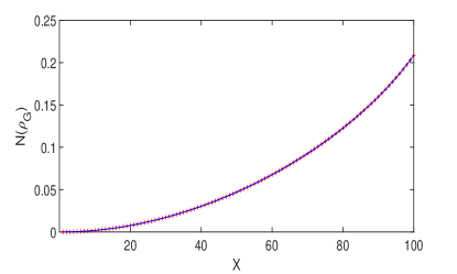
Figure 1: (color online) SMIN results for randomly generated states $\rho_{G}$ vs. $x$. The solid line corresponds to the strictly analytical expressions of Equation (6), (7) and (8), while the numerical solutions are marked with ”+” symbols.

Example 2.- The SQD of $(2\otimes 2)$-dimensional Werner states.

To demonstrate the validity of Theorem 2, we consider the Werner states. Werner states are the ”X”-type states expressed as

$$\rho_{W}=\frac{2-x}{6}\mathbb{I}_{4}+\frac{2x-1}{6}V,x\in[-1,1],$$ (52)

where $V=\sum_{kl}\left|kl\right\rangle\left\langle lk\right|$ denotes the swap operator. On the basis of our definition, the SQD $D(\rho_{W})$ can be calculated as

$$D(\rho_{AB})=\frac{1}{6}(2-x-\sqrt{3(1-x^{2})}).$$ (53)

For comparison, we plot both the analytical expression given in Equation (53) and the numerical results in Figure 2. Again, the analytical and numerical results show complete consistency.

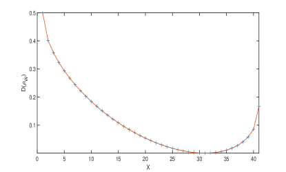
Figure 2: (color online) SQD results for Werner states vs. $x$. The solid line and the ”+” symbols correspond to the strictly analytical expression of Equation (53) and the numerical results, respectively.

Example 3.- The SQD of $(2\otimes 2)$-dimensional general quantum states

To further demonstrate the validity of our Theorem 2, we consider a general state, denoted by $\rho_{R}$, that has the same form as the state $\rho_{G}$ in Equation (51) but the matrix $G$ replaced by $R$, where the matrix $R=R_{1}+iR_{2}$, with

$$R_{1}=\left(\begin{array}[]{cccc}0.2481&0&0&0.0103\\ 0&0.2083&0.0285&0\\ 0&0.0285&0.4657&0\\ 0.0103&0&0&0.0779\end{array}\right),$$ (54)

$$R_{2}=\left(\begin{array}[]{cccc}0&0&0&-0.0141\\ 0&0&0.0877&0\\ 0&-0.0877&0&0\\ 0.0141&0&0&0\end{array}\right),$$ (55)

is a randomly generated ”X”-type state. We compare our analytical results for the SQD of such states with the numerical results in Figure 3 which again shows perfect consistency.

Figure 3: (color online) SQD results for ”X”-type states $\rho_{R}$ vs. $x$. The solid line corresponds to the strictly analytical expression of Equation (12), while the numerical solutions are marked with ”+” symbols.

Example 4.-The SQD of $(2\otimes 2)$-dimensional general block-diagonal states

To demonstrate the validity of our Theorem 3, we consider a state $\rho_{M}$ generated in the same way as that shown in Equation (51) but with $G$ replaced by $M$, where the matrix $M$ is constructed as the direct sum of two randomly generated $2\times 2$ matrices, i.e., $M=M_{1}\oplus M_{2}$, with

$$M_{1}=\left(\begin{array}[]{cc}0.3093&0.2321+0.0039i\\ 0.2321-0.0039i&0.1885\end{array}\right),$$ (56)

and

$$M_{2}=\left(\begin{array}[]{cc}0.1972&0.2075+0.1204i\\ 0.2075-0.1204i&0.3050\end{array}\right).$$ (57)

We plot the SQD results for such states $\rho_{M}$ as determined both numerically and analytically. The results are completely consistent with each other.

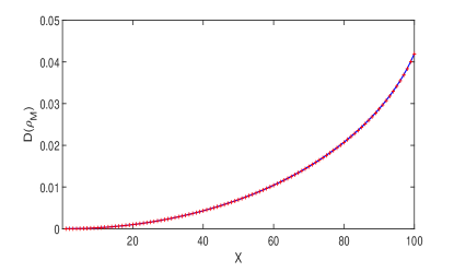
Figure 4: (color online) SQD results for block-diagonal states $\rho_{M}$ vs. $x$. The solid line corresponds to the strictly analytical expression of Equation (43), while the numerical solutions are marked with ”+” symbols.

V Conclusions and discussion

We have studied the symmetric quantum discord (SQD) and the symmetric measurement-induced nonlocality (SMIN) as defined in terms of the quantum skew information. It is shown that these two quantum correlations do not change when an additional state is attached to the state of interest. In particular, we find that the SMIN can be analytically calculated for any bipartite qubit states and that the SQD can be analytically calculated for two-qubit states of the ”X” type and of the block-diagonal form. Numerical tests are presented to demonstrate that our analytical expressions are valid. Since the derivation of analytical expressions for quantifiers of quantum resources is generally the main challenge in resource theory, we believe that our results could have broad applications in related studies.

Appendix A A useful lemma

Lemma: Let $A$ and $B$ be two nonnormalized qubit density matrices. There always exists a unitary operation $U$ such that $\left[UAU^{\dagger}\right]_{11}=\left[UAU^{\dagger}\right]_{22}$ and $\left[UBU^{\dagger}\right]_{11}=\left[UBU^{\dagger}\right]_{22}$ hold simultaneously.

Proof. Let the unitary matrix $U=\left(\begin{array}[]{cc}\cos\theta&e^{i\varphi}\sin\theta\\ -e^{-i\varphi}\sin\theta&\cos\theta\end{array}\right)$, and let $A^{\prime}=UAU^{\dagger}$ and $B^{\prime}=UBU^{\dagger}$. Then, the diagonal entries of $A^{\prime}$ and $B^{\prime}$ read

$$A_{11}^{\prime} = A_{11}\cos^{2}\theta+A_{22}\sin^{2}\theta$$

$$+(A_{12}e^{-i\varphi}+A_{21}e^{i\varphi})\cos\theta\sin\theta,$$

$$A_{22}^{\prime} = A_{11}\sin^{2}\theta+A_{22}\cos^{2}\theta$$

$$-(A_{12}e^{-i\varphi}+A_{21}e^{i\varphi})\cos\theta\sin\theta,$$

$$B_{11}^{\prime} = B_{11}\cos^{2}\theta+B_{22}\sin^{2}\theta$$

$$+(B_{12}e^{-i\varphi}+B_{21}e^{i\varphi})\cos\theta\sin\theta,$$

$$B_{22}^{\prime} = B_{11}\sin^{2}\theta+B_{22}\cos^{2}\theta$$ (58)

$$-(B_{12}e^{-i\varphi}+B_{21}e^{i\varphi})\cos\theta\sin\theta,$$

with $A_{ij}$ and $B_{ij}$, $i,j=1,2$, denoting the entries of the corresponding matrices. $A_{11}^{\prime}=A_{22}^{\prime}$ and $B_{11}^{\prime}=B_{22}^{\prime}$ imply that

$$(A_{11}-A_{22})\cos 2\theta$$ (59)

$$= -(A_{12}e^{-i\varphi}+A_{21}e^{i\varphi})\sin 2\theta,$$

and

$$(B_{11}-B_{22})\cos 2\theta$$ (60)

$$= -(B_{12}e^{-i\varphi}+B_{21}e^{i\varphi})\sin 2\theta.$$

From these two equations, one can easily find that $p\cos\varphi+q\sin\varphi=0$, where $p=(B_{11}-B_{22})(A_{12}+A_{21})-(A_{11}-A_{22})(B_{12}+B_{21})$ and $q=(B_{11}-B_{22})(A_{21}-A_{12})i-(A_{11}-A_{22})(B_{21}-B_{12})i$. Thus, we have

$$\tan\varphi=-\frac{p}{q}.$$ (61)

By substituting Equation (61) into Equation (59), one can obtain

$$\tan 2\theta=\frac{A_{11}-A_{22}}{A_{12}e^{-i\varphi_{2}}+A_{21}e^{i\varphi_{2}}}.$$ (62)

Thus, the proof is complete. $\blacksquare$

References

- (1) R. Horodecki, P. Horodecki, M. Horodecki, K. Horodecki, Rev. Mod. Phys. 2009, 81, 865.
- (2) K. Modi, A. Brodutch, H. Cable, T. Paterek, and V. Vedral, Rev. Mod. Phys. 2012, 84, 1655.
- (3) A. Streltsov, G. Adesso, M. B. Plenio, Rev. Mod. Phys. 2017, 89, 041003.
- (4) C. H. Bennett, H. J. Bernstein, S. Popescu, B. Schumacher, Phys. Rev. A 1996, 53, 2046.
- (5) C. H. Bennett, D. P. DiVincenzo, J. A. Smolin, W. K. Wootters, Phys. Rev. A 1996, 54, 3824.
- (6) W. K. Wootters, Phys. Rev. Lett. 1998, 80, 2245.
- (7) A. Peres, Phys. Rev. Lett. 1996, 77, 1413.
- (8) M. Horodecki, P. Horodecki, R. Horodecki, Phys. Lett. A 1996, 223, 1.
- (9) G. Vidal and R. F. Werner, Phys. Rev. A 2002, 65, 032314 .
- (10) W. Dür, G. Vidal, and J. I. Cirac, Phys. Rev. A 2000, 62, 062314.
- (11) A. Miyake, and F. Verstraete, Phys. Rev. A 2004, 69, 012101.
- (12) V. Coffman, J. Kundu, and W. K. Wootters, Phys. Rev. A 2000, 61, 052306.
- (13) G. Alber, T. Beth, M. Horodecki, P. Horodecki, R. Horodecki, M. Rötterler, H. Weinfurter, R. Werner, A. Zeilinger, Quantum information: An introduction to basic theoretical concepts and experiments, Springer-Verlag, Berlin Heidelberg, 2001.
- (14) L. E. Buchholz, T. Moroder, and O. Gühne, Ann. Phys. 2016, 528, 278.
- (15) S. M. Fei, J Jost, X. Q. Li, G. F. Wang, Phys. Lett. A 2003, 310, 333.
- (16) F. Mintert, M. Kuś, and A. Buchleitner, Phys. Rev. Lett. 2004, 92, 167902.
- (17) K. Chen, S. Albeverio, and S. M. Fei, Phys. Rev. Lett. 2005, 95, 040504.
- (18) G. Giedke, M. M. Wolf, O. Krüger, R. F. Werner, and J. I. Cirac, Phys. Rev. Lett. 2003, 91, 107901.
- (19) C. S. Yu, and H. S. Song, Phys. Rev. A 2005, 72, 022333.
- (20) R. Lohmayer, A. Osterloh, J. Siewert, and A. Uhlmann, Phys. Rev. Lett. 2006, 97, 260502.
- (21) F. Mintert, Phys. Rev. A 2007, 75, 052302.
- (22) J. Siewert and C. Eltschka, Phys. Rev. Lett. 2012, 108, 230502.
- (23) J. Sperling and W. Vogel, Phys. Rev. Lett. 2013, 111, 110503.
- (24) L. Henderson, V. Vedral, J. Phys. A:Math. Theor. 2001, 34, 6899.
- (25) H. Ollivier, W. H. Zurek, Phys. Rev. Lett. 2001, 88, 017901.
- (26) B. Dakic, V. Vedral, and C. Brukner, Phys. Rev. Lett. 2010, 105, 190502.
- (27) C. S. Yu, and H. Q. Zhao, Phys. Rev. A 2011, 84, 062123.
- (28) D. Girolami, T. Tufarelli, and G. Adesso, Phys. Rev. Lett. 2013, 110, 240402.
- (29) C. S. Yu, S. X. Wu, X. G. Wang, X. X. Yi and H. S. Song, Europhys. Lett. 2014, 107, 10007.
- (30) M. Rama, Front. Phys. 2016, 11, 111404.
- (31) R. Fan, P. Zhang, H. Shen, H. Zhai, Sci. Bull. 2017, 62, 707.
- (32) M. Zhao, T. Ma, T. Zhang, S. M. Fei, Sci. China-Phys. Mech. Astron. 2016, 59, 120313.
- (33) G. Y. Zhou, L. J. Huang, J. Y. Pan, L. Y. Hu, J. H. Huang, Frontiers of Physics 2018, 13, 130701.
- (34) J. BatleEmail, A. Farouk, O. Tarawneh, S. Abdalla, Frontiers of Physics 2018, 13, 130305.
- (35) H. Li, X. Gao, T. Xin, M. H. Yung, G. L. Long, Sci. Bull. 2017, 62, 497.
- (36) H. Wang, W. Zheng, N. Yu, K. Li, D. Lu, T. Xin, C. Li, Z. Ji, D. Kribs, B. Zeng, X. Peng, J. Du, Sci. China: Phys., Mech. Astron. 2016, 59, 100313.
- (37) Y. Huang, Phys. Rev. A 2013, 88, 014302.
- (38) N. Min, J. Chang, J. Shin, Y. Kwon, Int. J. Theor. Phys. 2015, 54, 3340.
- (39) T. Chanda, A. K. Pal, A. Biswas, A. Sen(De), U. Sen, Phys. Rev. A 2015, 91, 062119.
- (40) S. Luo, and S. Fu, Phys. Rev. Lett. 2011, 106, 120401.
- (41) S. X. Wu, J. Zhang, C. S. Yu, and H. S. Song, Phys. Lett. A 2014, 378, 344.
- (42) L. Q. Zhang, T. T. Ma, and C. S. Yu, Phys. Rev. A 2018, 97, 032112.
- (43) S. Luo, Phys. Rev. A 2008, 77, 042303.
- (44) S. Luo, and S. Fu, Phys. Rev. A 2010, 82, 034302.
- (45) K. Modi, T. Paterek, W. Son, V. Vedral, and M. Williamson, Phys. Rev. Lett. 2010, 104, 080501.
- (46) C. S. Yu, and H. Q. Zhao, Phys. Rev. A 2011, 84, 062123.
- (47) Q. Chen, C. Zhang, S. Yu, X. Yi, and C. H. Oh, Phys. Rev. A 2011, 84, 042313.
- (48) M. L. Hu, and H. Fan, New. J. Phys. 2015, 17, 033004.
- (49) J. Chen, C. Guo, Z. Ji, Y. T. Poon, N. Yu, B. Zeng, J. Zhou, Sci. China: Phys., Mech. Astron. 2017, 60, 020312.
- (50) J. Maziero, L. C. Céleri, R. M. Serra, arXiv:1004.2082. 2010.
- (51) F. J. Jiang, H. J. Lü, X. H. Yan and M. J. Shi, Chin. Phys. B 2013, 22, 040303.
- (52) J. Xu, Phys. Lett. A 2012, 376, 320.
- (53) C. S. Yu and H. S. Song, Phys. Rev. A 2009, 80, 022324.
- (54) C. S. Yu, Y. Zhang, H. Zhao, Quantum Inf. Process. 2014, 13, 1437.
- (55) T. Baumgratz, M. Cramer, and M. B. Plenio, Phys. Rev. Lett. 2014, 113, 140401.
- (56) A. Winter and D. Yang, Phys. Rev. Lett. 2016, 116, 120404.
- (57) E. Chitambar and M. H. Hsieh, Phys. Rev. Lett. 2016, 117, 020402.
- (58) A. Streltsov, S. Rana, P. Boes and J. Eisert, Phys. Rev. Lett. 2017, 119, 140402.
- (59) K. B. Dana, M. G. Díaz, M. Mejatty and A. Winter, Phys. Rev. A 2017, 95, 062327.
- (60) A. Streltsov, S. Rana, M. N. Bera and M. Lewenstein, Phys. Rev. X 2017, 7, 011024.
- (61) C. S. Yu, Phys. Rev. A 2017, 95, 042337.
- (62) F. G. S. L. Brandão, G. Gour, Phys. Rev. Lett. 2015, 115, 070503.
- (63) S. R. Yang, and C. S. Yu, Ann. Phys. 2018, 388, 305.
- (64) H. Q. Zhao, and C. S. Yu, Sci. Reps. 2018, 8, 299.
- (65) J. Ma, B. Yadin, D. Girolami, V. Vedral, M. Gu, Phys. Rev. Lett. 2016, 116, 160407.
- (66) Y. Sun, Y. Mao and S. Luo, Europhys. Lett. 2017, 118, 60007.
- (67) M. Piani, Phys. Rev. A 2012, 86, 034101.
- (68) T. Zhou, J. Cui, G. L. Long, Phys. Rev. A 2011, 84, 062105.
- (69) X. F. Qi, T. Gao, F. L. Yan, Frontiers of Physics 2018, 13, 130309.
- (70) T. Ma, M. J. Zhao, H. J. Zhang, S. M. Fei, G. L. Long, Phys. Rev. A 2017, 95, 042328.
- (71) E. P. Wigner and M. M. Yanase, Proc. Natl. Acad. Sci. U. S. A. 1963, 49, 910.
- (72) E. H. Lieb, Adv. Math. 1973, 11, 267.
- (73) S. Luo, Proc. Am. Math. Soc. 2004, 132, 885.
- (74) Z. H. Ma, Z. H. Chen, S. M. Fei, Sci. China-Phys. Mech. Astron. 2017, 60, 010321
- (75) G. H. Golub, C. F. Van Loan, Matrix Computations. 2nd ed. The John Hopkins University Press, Baltimore, 1989.