On the coherent states for a relativistic scalar particle

Abstract

The three approaches to relativistic generalization of coherent states are discussed in the simplest case of a spinless particle: the standard, canonical coherent states, the Lorentzian states and the coherent states introduced by Kaiser and independently by Twareque Ali, Antoine and Gazeau. All treatments utilize the Newton-Wigner localization and dynamics described by the Salpeter equation. The behavior of expectation values of relativistic observables in the coherent states is analyzed in detail and the Heisenberg uncertainty relations are investigated.

1 Introduction

In spite of the fact that coherent states are of fundamental importance in quantum physics, the problem of their relativistic generalization remains open. The difficulties in extending the concept of coherent states to the relativistic domain are related with problems in constructing relativistic quantum mechanics. In particular, they are connected with identification of the appropriate relativistic counterpart of the Schrödinger equation and corresponding position and momentum operators acting on a concrete Hilbert space. The most popular relativistic generalizations of the Schrödinger equation for the scalar massive particles are the Klein-Gordon equation [1, 2, 3, 4] and the less known “square root” of this equation usually referred to as the Salpeter equation [5, 6, 7, 8, 9, 10, 11, 12, 13, 14, 15, 16, 17, 18, 19, 20, 21, 22, 23, 24, 25, 26, 27, 28]. We remark that the latter equation appears in the context of the so called relativistic Hamiltonian dynamics [29, 30]. An asset of the Klein-Gordon equation is its manifest covariance. The grave flaw of this equation is the problem with probablistic interpretation, namely the probability density can be negative. To circumvent the problem the probability current is reinterpreted as a charge current. Furthermore, we deal with paradoxes such as “Zitterbewegung” and Klein paradox, connected with existence of solutions corresponding to negative energy. To bypass the problem one usually suggests the creation of particle-antiparticle pairs and conclude that there is no consistent one-particle relativistic quantum mechanics. The great advantage of the Salpeter equation is that it has well-defined probability density and current [25]. Recently, it has been demonstrated [31] that this current is consistent with relativistic generalization of the Wigner function [32]. Furthermore, the Salpeter equation possesses only positive energy solutions, so the paradoxes do not occur such as “Zitterbewegung” and Klein paradox mentioned earlier. Its flaw is that it is not manifestly covariant. Another problem that is sometimes pointed out is the nonlocality of the Hamiltonian referring to the Salpeter equation which is the pseudodifferential operator. In spite of its nonlocality, the Salpeter equation does not disturb the light cone structure and the second quantized version of this equation is macrocausal [12]. Despite its flaws, the advantages of the Salpeter equation were the reason for its wide usage in the description of the quark-antiquark gluon system [33, 34].

As far as we are aware the first example of relativistic coherent states in the literature were the states for a spin 0 and spin-1/2 charged particle in an external magnetic field discussed by Malkin and Man’ko in [35], and by Lev, Semenov, Usenko and Klauder in more recent papers [36, 37, 38]. The relativistic dynamics chosen in these papers is described by the Klein-Gordon equation or its matrix first-order counterpart introduced by Feshbach and Villars [39]. The problem with the introduced coherent states is, among others, their interpretation as the states closest to the classical ones. This issue is explicitly recognized in ref. 35. As a matter of fact the uncertainty relations were discussed in [38] where the Klein-Gordon equation on a “null” plane was utilized. Nevertheless, the condition for minimalization of these relations in coherent states found in [38] mixes temporal and spatial coordinates, so it is time-dependent in contrary to the fact that definition of coherent states should not depend on dynamics — they should be parametrized only by points of the phase space. Yet another example of relativistic coherent states based on the Klein-Gordon equation are the states introduced in [40].

In this work we discuss the coherent states for a spinless particle assuming the dynamics is described by the spinless Salpeter and the position and momentum operators have the corresponding $L^{2}$ representation. We study the three candidates for coherent states in relativistic quantum mechanics. The first ones are the standard, canonical coherent states that were not investigated in the relativistic context so far. We also study the states related to the exact solutions to the Salpeter equation referred in the massless case as to “Lorentzian” packages and the states introduced by Bakke and Wergeland [41, 42] and Kaiser [43] as well as independently by Twareque Ali, Antoine and Gazeau [44, 45]. We obtain, among others, the new formulas related to these coherent states and discuss the corresponding uncertainty relations.

2 Preliminaries

In this section we briefly sketch some basic facts about the Salpeter equation and the corresponding Hilbert space (see for example [23, 25]). Consider the Hamiltonian of a free relativistic classical particle

$$H=\sqrt{c^{2}{\bm{p}}^{2}+m^{2}c^{4}},$$ (2.1)

where $m$ is the mass of a particle, ${\bm{x}}$ is its three-position and $c$ is the speed of light. Applying to (2.1) the quantization procedure based on the Newton-Wigner localization scheme [6] using the standard Schrödinger quantization rule $\hat{\bm{x}}\to{\bm{x}}$, and $\hat{\bm{p}}\to-{\rm i}\hbar{\bm{\nabla}}$, we arrive at the Salpeter equation such that

$${\rm i}\hbar\frac{\partial\phi({\bm{x}},t)}{\partial t}=\sqrt{-\hbar^{2}c^{2}\Delta+m^{2}c^{4}}\phi({\bm{x}},t),$$ (2.2)

where the space of solutions to the Salpeter equation is $L^{2}(\mathbb{R}^{3},d^{3}{\bm{x}})$ specified by the scalar product

$$\langle\phi|\psi\rangle=\int d^{3}{\bm{x}}\,\phi^{*}({\bm{x}})\psi({\bm{x}}).$$ (2.3)

We point out that every solution of the Salpeter equation (2.2) is also the solution of the free Klein-Gordon equation. The opposite is clearly not true because of existence of negative energy solutions to the Klein-Gordon equation. For a more complete discussion of relations between the Salpeter and Klein-Gordon equation we refer the reader to [25].

On performing the Fourier transformation

$$\phi({\bm{x}},t)=\frac{1}{(2\pi)^{\frac{3}{2}}\hbar^{3}}\int d^{3}{\bm{p}}\,e^{{\rm i}\frac{{\bm{p}}\mbox{\boldmath$\scriptstyle{\cdot}$}{\bm{x}}}{\hbar}}\tilde{\phi}({\bm{p}},t),$$ (2.4)

we get the Salpeter equation in the momentum representation

$${\rm i}\hbar\frac{\partial\tilde{\phi}({\bm{p}},t)}{\partial t}=\sqrt{{\bm{p}}^{2}c^{2}+m^{2}c^{4}}\phi({\bm{p}},t),$$ (2.5)

where the space of solutions to (2.5) is the Hilbert space $L^{2}(\mathbb{R}^{3},d^{3}{\bm{p}})$ with the scalar product

$$\langle\phi|\psi\rangle=\frac{1}{\hbar^{3}}\int d^{3}{\bm{p}}\,{\tilde{\phi}}^{*}({\bm{p}}){\tilde{\psi}}({\bm{p}}).$$ (2.6)

Clearly, the action of position and momentum operators is given by the standard Schrödinger rule

$$\hat{\bm{x}}\tilde{\phi}({\bm{p}})={\rm i}\hbar{\bm{\nabla}}_{{\bm{p}}}\tilde{\phi}({\bm{p}}),\qquad\hat{\bm{p}}\tilde{\phi}({\bm{p}})={\bm{p}}\tilde{\phi}({\bm{p}}).$$ (2.7)

We remark that the measure $d^{3}{\bm{p}}$ is not invariant measure on a mass hyperboloid. The isomorphism of the Hilbert space specified by the scalar product (2.6) and the Hilbert space with the invariant measure $\frac{mc\,d^{3}{\bm{p}}}{p^{0}({\bm{p}})}$ such that

$$\langle\phi^{\prime}|\psi^{\prime}\rangle=\frac{1}{\hbar^{3}}\int\frac{mc\,d^{3}{\bm{p}}}{p^{0}({\bm{p}})}{\tilde{\phi}}^{\prime*}({\bm{p}}){\tilde{\psi}}^{\prime}({\bm{p}}),$$ (2.8)

where $p^{0}({\bm{p}})=\sqrt{{\bm{p}}^{2}+m^{2}c^{2}}$, is given by the transformation

$$\tilde{\phi}^{\prime}({\bm{p}})=\frac{1}{mc}\sqrt{p^{0}({\bm{p}})}\tilde{\phi}({\bm{p}}).$$ (2.9)

The position and momentum operators act in the Hilbert space with the scalar product (2.8) in the following way

$$\hat{\bm{x}}_{\rm NW}\tilde{\phi}^{\prime}({\bm{p}})=\left({\rm i}\hbar{\bm{\nabla}}_{{\bm{p}}}-\frac{{\rm i}\hbar}{2}\frac{{\bm{p}}}{{\bm{p}}^{2}+m^{2}c^{2}}\right)\tilde{\phi}^{\prime}({\bm{p}}),\qquad\hat{\bm{p}}\tilde{\phi}^{\prime}({\bm{p}})={\bm{p}}\tilde{\phi}^{\prime}({\bm{p}}).$$ (2.10)

We point out that our choice of rather nonstandard form of the invariant measure was motivated by limiting procedures in the nonrelativistic case and some dimensional deliberations. The position operator from the formula (2.10) is the well known Newton-Wigner operator. It should be noted that the Newton-Wigner operator is not covariant.

3 Standard coherent states in relativistic quantum mechanics

3.1 Standard coherent states

An experience with construction of the standard, canonical coherent states based on canonical commutation relations $[a,a^{\dagger}]=I$, and their numerous generalizations such as for example coherent states for a particle on a circle, sphere and torus [46, 47, 48, 49] shows that one of their most important property is not a temporal stability with respect to some particular evolution but the parametrization by points of the classical phase space. On the other hand, we have the standard $L^{2}$ Schrödinger realization of the space of solutions to the Salpeter equation described in the previous section. Therefore, it seems plausible to discuss the possibility of applying the canonical coherent states also in relativistic case. Of course the canonical coherent states are not Lorentz covariant and should be defined in a concrete reference frame. Nevertheless, it is interesting to compare the behavior of average of relativistic observables in these states and covariant ones. Consider the canonical coherent states. We restrict for simplicity to the one-dimensional configuration space. These states are eigenvectors of the annihilation operator

$$\hat{a}|z\rangle=z|z\rangle,$$ (3.1)

where

$$\hat{a}=\frac{1}{\sqrt{2}}\left(\frac{\hat{x}}{\sigma}+{\rm i}\frac{\sigma\hat{p}}{\hbar}\right)$$ (3.2)

and $\sigma$ is a constant with dimension of length. In the case of the harmonic oscillator coherent states we have $\sigma=\sqrt{\hbar/m\omega}$. The complex number $z$ labelling the coherent states can be expressed by means of the average position $\bar{x}=\langle z|\hat{x}|z\rangle$ and momentum $\bar{p}=\langle z|\hat{p}|z\rangle$ in the form

$$z=\frac{1}{\sqrt{2}}\left(\frac{\bar{x}}{\sigma}+{\rm i}\frac{\sigma\bar{p}}{\hbar}\right).$$ (3.3)

The standard deviations in the coherent state $|z\rangle$ satisfy

$$\Delta\hat{x}=\frac{\sigma}{\sqrt{2}},\qquad\Delta\hat{p}=\frac{\hbar}{\sqrt{2}\sigma},\qquad\Delta\hat{x}\Delta\hat{p}=\frac{\hbar}{2},$$ (3.4)

so the coherent states minimalize the Heisenberg uncertainty relations. In this sense the coherent states are closest to the classical ones. The coherent states are not orthogonal. We have

$$\langle z|w\rangle=\exp[-\textstyle{\frac{1}{2}}(|z|^{2}+|w|^{2}-2z^{*}w)].$$ (3.5)

The coherent states form the complete (overcomplete) set. Namely,

$$\frac{1}{\pi}\int d{\rm Re}z\,d{\rm Im}z\,|z\rangle\langle z|=I,$$ (3.6)

or equivalently

$$\frac{1}{2\pi\hbar}\int d\bar{x}d\bar{p}\,|\bar{x},\bar{p}\rangle\langle\bar{x},\bar{p}|=I,$$ (3.7)

where $|\bar{x},\bar{p}\rangle\equiv|z\rangle$, with $z$ expressed by (3.3).

Consider now the one-dimensional counterpart of the momentum representation specified by (2.6) and (2.7)

$$\langle\phi|\psi\rangle =\frac{1}{\hbar}\int dp\,{\tilde{\phi}}^{*}(p)\tilde{\psi}(p),$$ (3.8)

$$\hat{x}\tilde{\phi}(p) ={\rm i}\hbar\frac{\partial\tilde{\phi}}{\partial p},\qquad\hat{p}\tilde{\phi}(p)=p\tilde{\phi}(p),$$ (3.9)

where $\tilde{\phi}(p)=\langle p|\phi\rangle$, and the vectors $|p\rangle$ span the momentum representation.

The normalized coherent states in the momentum representation are given by

$$\tilde{\phi}_{z}(p) =\frac{\sigma^{\frac{1}{2}}}{\pi^{\frac{1}{4}}}e^{\textstyle{\frac{1}{2}}(z^{2}-|z|^{2})}e^{-\textstyle{\frac{1}{2}}\frac{\sigma^{2}p^{2}}{\hbar^{2}}-\frac{{\rm i}\sqrt{2}z\sigma p}{\hbar}},$$ (3.10)

$$\tilde{\phi}_{z}(p) =\frac{\sigma^{\frac{1}{2}}}{\pi^{\frac{1}{4}}}\exp\left[-\frac{\sigma^{2}}{2\hbar^{2}}(p-\bar{p})^{2}-{\rm i}\frac{{\bar{x}}p}{\hbar}\right],$$ (3.11)

where $\tilde{\phi}_{z}(p)=\langle p|z\rangle\equiv\langle p|\bar{x},\bar{p}\rangle$, and $z$ is given by (3.3).

We finally write down the formula for the average value of the energy of the free nonrelativistic particle such that

$$\bar{E}=\langle z|\frac{{\hat{p}}^{2}}{2m}|z\rangle=\frac{{\bar{p}}^{2}}{2m}+\frac{\hbar^{2}}{4\sigma^{2}m}.$$ (3.12)

Thus, up to additive constant, we have the classical relation between the average energy and momentum of a particle. An experience with coherent states for a particle on a circle and sphere [46, 47] shows that such behavior is one of characteristic properties of coherent states.

3.2 Averages of relativistic observables in the canonical coherent states

We now investigate the closeness of the canonical coherent states to the classical phase space in the relativistic case by means of the analysis of averages of relativistic observables in these states. Consider the Hamiltonian of a free relativistic particle

$$H=\sqrt{c^{2}{\hat{p}}^{2}+m^{2}c^{4}}.$$ (3.13)

Using (3.8), (3.9) and (3.11) we find that the average energy in the canonical coherent state is

$$\bar{E}=\langle z|\sqrt{c^{2}{\hat{p}}^{2}+m^{2}c^{4}}|z\rangle=\frac{\sigma}{\sqrt{\pi}\hbar}\int_{-\infty}^{\infty}e^{-\frac{\sigma^{2}}{\hbar^{2}}(p-\bar{p})^{2}}\sqrt{c^{2}p^{2}+m^{2}c^{4}}\,dp.$$ (3.14)

Expanding the exponential function in (3.14) into the power series and using the identity

$$\int_{-\infty}^{\infty}e^{-\beta x^{2}}\sqrt{x^{2}+\gamma^{2}}\,dx=\frac{\sqrt{\pi}}{\beta}U(-\textstyle{\frac{1}{2}},0,\beta\gamma^{2}),\quad{\rm Re}\beta>0,\quad{\rm Re}\gamma^{2}>0,$$ (3.15)

where $U(a,b,z)$ is the confluent hypergeometric function [50], and (A2) and (A3), we get the following power series representation of the integral from (3.14)

$$\bar{E}=\frac{c\hbar}{\sigma}e^{-\left(\frac{\sigma\bar{p}}{\hbar}\right)^{2}}\sum_{n=0}^{\infty}\frac{1}{n!}\left(\frac{\sigma\bar{p}}{\hbar}\right)^{2n}U\left[-\frac{1}{2},-n,\left(\frac{\sigma}{\lambda_{c}}\right)^{2}\right],$$ (3.16)

where $\lambda_{c}=\frac{\hbar}{mc}$ is the Compton wavelength. The numerical calculations based on (3.14) or (3.16) show that for $\sigma/\lambda_{c}\geqslant 5$ (the larger fraction the better approximation) we have an approximate relation

$$\bar{E}\approx\sqrt{{\bar{p}}^{2}c^{2}+m^{2}c^{4}},$$ (3.17)

where the approximation is very good. Namely, for $\sigma/\lambda_{c}=5$ the maximal relative error $(\bar{E}-\sqrt{{\bar{p}}^{2}c^{2}+m^{2}c^{4}})/\bar{E}$ arising for $\bar{p}=0$ is of order 1%. We point out that $\sigma=5\lambda_{c}$ is still the length scale when the description is adequate based on relativistic quantum mechanics. This means that the parameter $\bar{p}$ labelling the coherent states can be regarded as the classical momentum also in the relativistic case.

We now discuss the case of a massless relativistic particle. The Hamiltonian (3.13) takes the form

$$H=c|\hat{p}|.$$ (3.18)

Taking into account (3.8) and (3.11) we get

$$\bar{E}=\langle z|c|\hat{p}||z\rangle=\frac{\sigma}{\sqrt{\pi}\hbar}\int_{-\infty}^{\infty}|p|e^{-\frac{\sigma^{2}}{\hbar^{2}}(p-\bar{p})^{2}}dp.$$ (3.19)

Hence, using the identity [51]

$$\int_{0}^{\infty}xe^{-\mu x^{2}-2\nu x}dx= \frac{1}{2\mu}-\frac{\nu}{2\mu}\sqrt{\frac{\pi}{\mu}}e^{\frac{\nu^{2}}{\mu}}\left[1-{\rm erf}\left(\frac{\nu}{\sqrt{\mu}}\right)\right],$$

$$\Big{|}{\rm arg}\nu<\frac{\pi}{2}\Big{|},\quad{\rm Re}\mu>0,$$ (3.20)

where ${\rm erf}(x)$ is the error function, we find

$$\bar{E}=c{\bar{p}}{\rm erf}\left(\frac{\sigma\bar{p}}{\hbar}\right)+\frac{c\hbar}{\sqrt{\pi}\sigma}e^{-\left(\frac{\sigma\bar{p}}{\hbar}\right)^{2}}.$$ (3.21)

Since ${\rm erf}(x)$ is an odd function we have

$$\bar{E}=c|{\bar{p}}|{\rm erf}\left(\frac{\sigma|\bar{p}|}{\hbar}\right)+\frac{c\hbar}{\sqrt{\pi}\sigma}e^{-\left(\frac{\sigma\bar{p}}{\hbar}\right)^{2}}.$$ (3.22)

From numerical simmulations we find that whenever $\sigma/{\bar{\lambda}}\geqslant 0.21$, where $|\bar{p}|=h/{\bar{\lambda}}$, and $h=2\pi\hbar$ is the Planck constant, which leads to $\bar{\lambda}\leqslant 4.76\sigma$, then we have

$$\bar{E}\approx c|\bar{p}|.$$ (3.23)

where the approximation is very good. Therefore, the parameter $\bar{p}$ marking the coherent states can be interpreted as the classical momentum of a massless particle. We point out that the condition $\bar{\lambda}\leqslant 4.76\sigma$ implies for the value of $\sigma$ analogous to that applied in the massive case such that $\sigma=5\lambda_{c}^{(\pi^{+})}$, where $\lambda_{c}^{(\pi^{+})}$ is the Compton wavelength of pion $\pi^{+}$, the estimate $\bar{\lambda}\leqslant 4{\cdot}10^{-5}\,{\rm nm}$. The value $4{\cdot}10^{-5}\,{\rm nm}$ corresponds to gamma rays. This result seems to be reasonable from the physical point of view.

Consider finally the expectation value of the operator of the relativistic velocity

$$\hat{v}=\frac{c\hat{p}}{\sqrt{{\hat{p}}^{2}+m^{2}c^{2}}}.$$ (3.24)

On taking into account (3.8) and (3.11) we arrive at the following formula for the average velocity

$$\bar{v}=\langle z|\hat{v}|z\rangle=\frac{c\sigma}{\sqrt{\pi}\hbar}\int_{-\infty}^{\infty}\frac{p}{\sqrt{p^{2}+m^{2}c^{2}}}e^{-\frac{\sigma^{2}}{\hbar^{2}}(p-{\bar{p}})^{2}}dp.$$ (3.25)

Hence, integrating by parts and using (3.14) we obtain

$$\bar{v}=\frac{\partial\bar{E}}{\partial\bar{p}}.$$ (3.26)

Thus, it turns out that $\bar{v}$ satisfies the classical relation. On the other hand, an immediate consequence of (3.16), (3.26) and (A3) is the power series expansion for $\bar{v}$ of the form

$$\bar{v}=ce^{-\left(\frac{\sigma\bar{p}}{\hbar}\right)^{2}}\sum_{n=0}^{\infty}\frac{1}{n!}\left(\frac{\sigma\bar{p}}{\hbar}\right)^{2n+1}U\left[\frac{1}{2},-n,\left(\frac{\sigma}{\lambda_{c}}\right)^{2}\right].$$ (3.27)

The numerical calculation based on (3.25) or (3.27) show that

$$\bar{v}\approx\frac{c\bar{p}}{\sqrt{{\bar{p}}^{2}+m^{2}c^{2}}},$$ (3.28)

where the approximation is as good as for (3.17) provided $\sigma/\lambda_{c}\geqslant 8$. This observation confirms once more that the parameter $\bar{p}$ marking the coherent states can be regarded as the classical relativistic momentum.

4 Lorentzian coherent states

4.1 Lorentzian coherent states

We now discuss the second candidate for relativistic coherent states — the momentum-space wave functions of the form

$$\tilde{\phi}(p)=C\exp(-\alpha\sqrt{p^{2}+m^{2}}+\beta p),$$ (4.1)

where $\alpha>|{\rm Re}\beta|$, $\hbar=1$, $c=1$, and $C$ is a normalization constant, and it is assumed that the Hilbert space is specified by (3.8). The wave functions (4.1) for $\beta=0$ were utilized in [25] and [52] for constructing the explicit solution to the free Salpeter equation

$${\rm i}\frac{\partial\tilde{\phi}(p,t)}{\partial t}=\sqrt{p^{2}+m^{2}}\tilde{\phi}(p,t),$$ (4.2)

where $\hbar=c=1$, in the momentum representation. Namely, we have

$$\tilde{\phi}(p,t)=C\exp[-(\alpha+{\rm i}t)\sqrt{p^{2}+m^{2}}].$$ (4.3)

The denomination “Lorentzian” was introduced by Rosenstein and Horwitz [53] who used it for the wave function (4.1) with $m=0$ and $\beta=0$. On performing the inverse Fourier transformation one can easily obtain the solution to the free particle Salpeter equation in the coordinate representation. The conterpart of the wave functions (4.1) in the case of the Dirac equation was discussed in [54] in the context of the quantum walks. The interpretation of the Lorentzian wave packets (4.1) as relativistic coherent states is supported by observations of Al-Hashimi and Wiese [55] who considered the general case with $\beta\neq 0$ and showed that these states minimalize the position-velocity uncertainty relations. In spite of this result the arising possibility of interpreting (4.1) as coherent states was not analyzed in [55]. In particular, the closeness of the Lorentzian states (4.1) to the classical ones connected with the parametrization of the phase space was not investigated therein.

Now, the form of (4.1) indicates that it can be regarded as a relativistic generalization of (3.11). Indeed, applying the Thiemann complexifier method [56] we can write the annihilation operator (3.2) as

$$\hat{a}=\frac{1}{\sqrt{2}}e^{-\frac{\sigma^{2}{\hat{p}}^{2}}{2\hbar^{2}}}\frac{\hat{x}}{\sigma}e^{\frac{\sigma^{2}{\hat{p}}^{2}}{2\hbar^{2}}}.$$ (4.4)

This operator is the nonrelativistic limit of the following one

$$\hat{b}=\frac{1}{\sqrt{2}}e^{-\frac{\sigma^{2}\sqrt{{\hat{p}}^{2}+m^{2}c^{2}}}{\lambda_{c}\hbar}}\frac{\hat{x}}{\sigma}e^{\frac{\sigma^{2}\sqrt{{\hat{p}}^{2}+m^{2}c^{2}}}{\lambda_{c}\hbar}},$$ (4.5)

where $\lambda_{c}=\hbar/mc$ is the Compton wavelength. An immediate consequence of (4.5) is

$$\hat{b}=\frac{1}{\sqrt{2}}\left(\frac{\hat{x}}{\sigma}+{\rm i}\frac{\sigma}{\lambda_{c}}\frac{\hat{p}}{\sqrt{{\hat{p}}^{2}+m^{2}c^{2}}}\right).$$ (4.6)

Hence, we finally get

$$\hat{b}=\frac{1}{\sqrt{2}}\left(\frac{\hat{x}}{\sigma}+{\rm i}\frac{\sigma}{\lambda_{c}}\frac{\hat{v}}{c}\right),$$ (4.7)

where $\hat{v}$ is the operator of the relativistic velocity given by (3.31). Now, as with (3.1) we define the coherent states as eigenvectors of the operator $\hat{b}$

$$\hat{b}|\zeta\rangle=\zeta|\zeta\rangle,$$ (4.8)

where $\zeta$ is a complex number. Analogously as in the case of the canonical coherent states discussed in the previous section we can express the complex number $\zeta$ with the help of average position $\bar{x}~{}=~{}\langle\zeta|\hat{x}|\zeta\rangle$ and average velocity $\bar{v}~{}=~{}\langle\zeta|\hat{v}|\zeta\rangle$, where $|\zeta\rangle$ is a normalized coherent state. Namely, we have

$$\zeta=\frac{1}{\sqrt{2}}\left(\frac{\bar{x}}{\sigma}+{\rm i}\frac{\sigma}{\lambda_{c}}\frac{\bar{v}}{c}\right).$$ (4.9)

The variations in the coherent state $|\zeta\rangle$ fulfil

$$(\Delta\hat{x})^{2} =-{\rm i}\frac{\sigma^{2}}{2\lambda_{c}c}\langle\zeta|[\hat{x},\hat{v}]|\zeta\rangle,$$ (4.10)

$$(\Delta\hat{v})^{2} =-{\rm i}\frac{c\lambda_{c}}{2\sigma^{2}}\langle\zeta|[\hat{x},\hat{v}]|\zeta\rangle.$$ (4.11)

Therefore

$$(\Delta\hat{x})^{2}(\Delta\hat{v})^{2}=\textstyle{\frac{1}{4}}|\langle\zeta|[\hat{x},\hat{v}]|\zeta\rangle|^{2}.$$ (4.12)

It thus appears that the states $|\zeta\rangle$ minimalize the Robertson position-velocity uncertainty relation

$$(\Delta\hat{x})^{2}(\Delta\hat{v})^{2}\geqslant\textstyle{\frac{1}{4}}|\langle\zeta|[\hat{x},\hat{v}]|\zeta\rangle|^{2}.$$ (4.13)

We now return to (4.8). On writing this equation in the momentum representation (see (3.9)) we arrive at the following momentum-space wave function representing the coherent state

$${\tilde{\phi}}_{\zeta}(p)=C\exp\left[-\frac{\sigma^{2}}{\lambda_{c}\hbar}\sqrt{p^{2}+m^{2}c^{2}}-{\rm i}\frac{\sqrt{2}\sigma\zeta}{\hbar}p\right],$$ (4.14)

where $C$ is a normalization constant. Thus, it turns out that the abstract coherent states defined by (4.8) coincide with the Lorentzian wave functions (4.1) with fixed values of the parameters $\alpha$ and $\beta$ specified by (4.14). We point out that the states (4.1) were derived in [54] in a more complicated way by demanding minimization of the Heisenberg uncertainty relation for position and velocity (4.13). Using the identity [57]

$$\int_{0}^{\infty}\exp(-\mu\sqrt{x^{2}+\nu^{2}})\cosh\rho x\,dx= \frac{\mu\nu}{\sqrt{\mu^{2}-\rho^{2}}}K_{1}(\nu\sqrt{\mu^{2}-\rho^{2}}),$$

$${\rm Re}\mu>|{\rm Re}\rho|,\quad{\rm Re}\nu>0,$$ (4.15)

where $K_{\nu}(z)$ is the modified Bessel function (Macdonald function), we find that the normalization constant $C$ in (4.14) is given by

$$C^{2}=\frac{\lambda_{c}\sqrt{1+\left(\frac{\lambda_{c}}{\sigma}\right)^{2}\left(\frac{\zeta-\zeta^{*}}{\sqrt{2}}\right)^{2}}}{2K_{1}\left[2\left(\frac{\sigma}{\lambda_{c}}\right)^{2}\sqrt{1+\left(\frac{\lambda_{c}}{\sigma}\right)^{2}\left(\frac{\zeta-\zeta^{*}}{\sqrt{2}}\right)^{2}}\right]}.$$ (4.16)

On the other hand, it appears that we have restriction on the complex number $\zeta$ parametrizing coherent states imposed by the first inequality from (4.15). Namely,

$$|\zeta-\zeta^{*}|<\sqrt{2}\frac{\sigma}{\lambda_{c}}.$$ (4.17)

Making use of (4.9) we can parametrize the coherent states by $\bar{x}$ and $\bar{v}$, so

$${\tilde{\phi}}_{\zeta}(p)=C\exp\left[-\frac{\sigma^{2}}{\lambda_{c}\hbar}\sqrt{p^{2}+m^{2}c^{2}}-{\rm i}\frac{\sigma}{\hbar}\left(\frac{\bar{x}}{\sigma}+{\rm i}\frac{\sigma}{\lambda_{c}}\frac{\bar{v}}{c}\right)p\right],$$ (4.18)

and

$$C^{2}=\frac{\lambda_{c}\sqrt{1-\left(\frac{\bar{v}}{c}\right)^{2}}}{2K_{1}\left[2\left(\frac{\sigma}{\lambda_{c}}\right)^{2}\sqrt{1-\left(\frac{\bar{v}}{c}\right)^{2}}\right]}.$$ (4.19)

The restriction (4.17) on $\zeta$ takes the simple, physically meaningful form

$$\Big{|}\frac{\bar{v}}{c}\Big{|}<1.$$ (4.20)

Now we are in a position to calculate the variances of the position and momentum in the coherent states. Taking into account (4.18) and the identity [57]

$$\int_{0}^{\infty}\frac{\exp(-\mu\sqrt{x^{2}+\nu^{2}})}{\sqrt{x^{2}+\nu^{2}}}\cosh\rho x\,dx= K_{0}(\nu\sqrt{\mu^{2}-\rho^{2}}),$$

$${\rm Re}\mu>|{\rm Re}\rho|,\quad{\rm Re}\nu>0,$$ (4.21)

we get

$$|\langle\zeta|[\hat{x},\hat{v}]|\zeta\rangle|= \frac{2\sigma^{2}c}{\lambda_{c}}\left\{1-\left(\frac{\bar{v}}{c}\right)^{2}-\frac{2\left(\frac{\sigma}{\lambda_{c}}\right)^{2}\sqrt{1-\left(\frac{\bar{v}}{c}\right)^{2}}}{K_{1}\left[2\left(\frac{\sigma}{\lambda_{c}}\right)^{2}\sqrt{1-\left(\frac{\bar{v}}{c}\right)^{2}}\right]}\right.$$

$$\times\left.\int_{1}^{\infty}K_{0}\left[2\left(\frac{\sigma}{\lambda_{c}}\right)^{2}\sqrt{\xi^{2}-\left(\frac{\bar{v}}{c}\right)^{2}}\right]d\xi\right\}.$$ (4.22)

Eqs. (4.10), (4.11) and (4.22) taken together yield

$$(\Delta\hat{x})^{2}= \frac{\sigma^{4}}{\lambda_{c}^{2}}\left\{1-\left(\frac{\bar{v}}{c}\right)^{2}-\frac{2\left(\frac{\sigma}{\lambda_{c}}\right)^{2}\sqrt{1-\left(\frac{\bar{v}}{c}\right)^{2}}}{K_{1}\left[2\left(\frac{\sigma}{\lambda_{c}}\right)^{2}\sqrt{1-\left(\frac{\bar{v}}{c}\right)^{2}}\right]}\right.$$

$$\times\left.\int_{1}^{\infty}K_{0}\left[2\left(\frac{\sigma}{\lambda_{c}}\right)^{2}\sqrt{\xi^{2}-\left(\frac{\bar{v}}{c}\right)^{2}}\right]d\xi\right\},$$ (4.23)

$$(\Delta\hat{v})^{2}= c^{2}\left\{1-\left(\frac{\bar{v}}{c}\right)^{2}-\frac{2\left(\frac{\sigma}{\lambda_{c}}\right)^{2}\sqrt{1-\left(\frac{\bar{v}}{c}\right)^{2}}}{K_{1}\left[2\left(\frac{\sigma}{\lambda_{c}}\right)^{2}\sqrt{1-\left(\frac{\bar{v}}{c}\right)^{2}}\right]}\right.$$

$$\times\left.\int_{1}^{\infty}K_{0}\left[2\left(\frac{\sigma}{\lambda_{c}}\right)^{2}\sqrt{\xi^{2}-\left(\frac{\bar{v}}{c}\right)^{2}}\right]d\xi\right\}.$$ (4.24)

We point out that in opposition to the case of the canonical coherent states (see (3.4)), the variances (4.23) and (4.24) depend on the parameter $\bar{v}$ labelling the Lorentzian coherent states. The scalar product of coherent states calculated with the help of (3.8), (4.14) and (4.15) is of the form

$$\langle\zeta|\eta\rangle=\frac{A(\zeta)A(\eta)}{\sqrt{1+\left(\frac{\lambda_{c}}{\sigma}\right)^{2}\left(\frac{\zeta^{*}-\eta}{\sqrt{2}}\right)^{2}}}K_{1}\left[2\left(\frac{\sigma}{\lambda_{c}}\right)^{2}\sqrt{1+\left(\frac{\lambda_{c}}{\sigma}\right)^{2}\left(\frac{\zeta^{*}-\eta}{\sqrt{2}}\right)^{2}}\right],$$ (4.25)

where

$$A^{2}(\zeta)=\frac{\sqrt{1+\left(\frac{\lambda_{c}}{\sigma}\right)^{2}\left(\frac{\zeta-\zeta^{*}}{\sqrt{2}}\right)^{2}}}{K_{1}\left[2\left(\frac{\sigma}{\lambda_{c}}\right)^{2}\sqrt{1+\left(\frac{\lambda_{c}}{\sigma}\right)^{2}\left(\frac{\zeta-\zeta^{*}}{\sqrt{2}}\right)^{2}}\right]}$$ (4.26)

and we have restriction on $\zeta$ and $\eta$ (see (4.15)) such that

$$\bigg{|}{\rm Re}\left[{\rm i}\frac{\lambda_{c}}{\sigma}\frac{1}{\sqrt{2}}(\zeta^{*}-\eta)\right]\bigg{|}<1$$ (4.27)

leading to

$$\Big{|}\frac{\bar{v}}{c}+\frac{\bar{v}^{\prime}}{c}\Big{|}<2,$$ (4.28)

where $\zeta=\frac{1}{\sqrt{2}}\left(\frac{\bar{x}}{\sigma}+{\rm i}\frac{\sigma}{\lambda_{c}}\frac{\bar{v}}{c}\right)$ and $\eta=\frac{1}{\sqrt{2}}\left(\frac{\bar{x}^{\prime}}{\sigma}+{\rm i}\frac{\sigma}{\lambda_{c}}\frac{\bar{v}^{\prime}}{c}\right)$. Notice that (4.28) is implied by $\big{|}\frac{\bar{v}}{c}\big{|}<1$, $\big{|}\frac{\bar{v}^{\prime}}{c}\big{|}<1$ and the triangle inequality. We also point out that non-orthogonality of coherent states is one of their most characteristic properties.

4.2 Averages of relativistic observables in the Lorentzian coherent states

In order to study the closeness of the discussed Lorentzian coherent states to the classical ones we now analyze averages of relativistic observables. We first discuss the expectation value of the momentum. An easy calculation based on (3.8), (3.9), (4.15), (4.18) and elementary properties of the Bessel functions gives

$$\bar{p}=\langle\zeta|\hat{p}|\zeta\rangle=\frac{m\bar{v}}{\sqrt{1-\left(\frac{\bar{v}}{c}\right)^{2}}}\frac{K_{2}\left[2\left(\frac{\sigma}{\lambda_{c}}\right)^{2}\sqrt{1-\left(\frac{\bar{v}}{c}\right)^{2}}\right]}{K_{1}\left[2\left(\frac{\sigma}{\lambda_{c}}\right)^{2}\sqrt{1-\left(\frac{\bar{v}}{c}\right)^{2}}\right]}.$$ (4.29)

From numerical calculations it follows that for sufficiently large $\sigma/\lambda_{c}$

$$\bar{p}\approx\frac{m\bar{v}}{\sqrt{1-\left(\frac{\bar{v}}{c}\right)^{2}}},$$ (4.30)

so we can interpret $\bar{v}$ labelling the coherent states as the classical relativistic velocity. The approximation (4.30) is as good as in the case of the average relativistic velocity in canonical coherent states analyzed in the previous section (see (3.31)). Namely (4.30) holds with relative error of order 1% for $\sigma/\lambda_{c}\geqslant 8$. We point out that in opposition to the standard coherent states applied for a relativistic particle discussed in the previous section, the constant $\sigma$ refers to the nonrelativistic case. Nevertheless, taking for example $\sigma~{}=~{}8\lambda_{c}^{(\pi^{+})}$, where $\sigma~{}=~{}\sqrt{\hbar/m\omega}$ is a characteristic oscillator length utilized in the definition of the nonrelativistic harmonic oscillator coherent states, and $\lambda_{c}^{(\pi^{+})}$ is the Compton wavelength of pion $\pi^{+}$, we get $\omega=3.2{\cdot}10^{21}\,\,{\rm Hz}$. This value is about one-half of the frequency $\omega_{\rm U}=6.9{\cdot}10^{21}\,\,{\rm Hz}$ of the wave-function oscillations corresponding to first orbital of a single electron and nucleus of Uranium, so it is physically meaningful.

We now study the average value of the energy in the Lorentzian coherent state. Making use of (3.8), (3.9), (4.18), (4.29) and elementary properties of the Bessel functions we find

$$\bar{E}=\langle\zeta|\sqrt{c^{2}{\hat{p}}^{2}+m^{2}c^{4}}|\zeta\rangle= \frac{mc^{2}}{\sqrt{1-\left(\frac{\bar{v}}{c}\right)^{2}}}\frac{K_{2}\left[2\left(\frac{\sigma}{\lambda_{c}}\right)^{2}\sqrt{1-\left(\frac{\bar{v}}{c}\right)^{2}}\right]}{K_{1}\left[2\left(\frac{\sigma}{\lambda_{c}}\right)^{2}\sqrt{1-\left(\frac{\bar{v}}{c}\right)^{2}}\right]}$$

$$-\frac{1}{2}\left(\frac{\lambda_{c}}{\sigma}\right)^{2}mc^{2}.$$ (4.31)

Numerical calculations show that as with the average momentum, whenever $\sigma/\lambda_{c}\geqslant 8$, then we have the approximate formula

$$\bar{E}\approx\frac{mc^{2}}{\sqrt{1-\left(\frac{\bar{v}}{c}\right)^{2}}},$$ (4.32)

where the approximation is as good as in (4.30). This observation confirms once more that $\bar{v}$ can be identified with the classical relativistic velocity.

The formulas for the averages (4.29) and (4.31) are most probably new. An equivalent but more complicated form of these relations was obtained in [55], where the parametrization was used by means of the Bessel functions $K_{0}(z)$ and $K_{1}(z)$ instead of $K_{1}(z)$ and $K_{2}(z)$.

We finally remark that the construction of Lorentzian coherent states introduced in this section cannot be applied in the case of the massless particles. Indeed, on the one hand, in the case of massless particles there is no nonrelativistic limit. On the other hand, we have no classical formulae relating for instance energy or momentum of a massless particle to its velocity. Therefore, the application of the Lorentzian coherent states labelled by classical velocities instead of momenta appears limited to the massive case. Clearly, the Lorentzian wave functions (4.1) can be studied in the limit $m=0$ without reference to the theory of coherent states as was done for example in [23] and [55].

4.3 Position-momentum uncertainty relations in the Lorentzian coherent states

Our purpose now is the analysis of the uncertainty relations between position and momentum in the Lorentzian coherent states. Proceeding analogously as with (4.29) the following formula for the average value of the squared momentum can be easily obtained

$${\bar{p}^{2}}= \langle\zeta|{\hat{p}}^{2}|\zeta\rangle$$

$$=\left[\frac{m\bar{v}}{\sqrt{1-\left(\frac{\bar{v}}{c}\right)^{2}}}\right]^{2}+\frac{(mc)^{2}}{2}\left(\frac{\lambda_{c}}{\sigma}\right)^{2}\frac{1+3\left(\frac{\bar{v}}{c}\right)^{2}}{\left[1-\left(\frac{\bar{v}}{c}\right)^{2}\right]^{\frac{3}{2}}}\frac{K_{2}\left[2\left(\frac{\sigma}{\lambda_{c}}\right)^{2}\sqrt{1-\left(\frac{\bar{v}}{c}\right)^{2}}\right]}{K_{1}\left[2\left(\frac{\sigma}{\lambda_{c}}\right)^{2}\sqrt{1-\left(\frac{\bar{v}}{c}\right)^{2}}\right]}.$$ (4.33)

Eqs. (4.29) and (4.33) taking together yield

$$(\Delta\hat{p})^{2}= \left[\frac{m\bar{v}}{\sqrt{1-\left(\frac{\bar{v}}{c}\right)^{2}}}\right]^{2}\left[1-\left(\frac{K_{2}\left[2\left(\frac{\sigma}{\lambda_{c}}\right)^{2}\sqrt{1-\left(\frac{\bar{v}}{c}\right)^{2}}\right]}{K_{1}\left[2\left(\frac{\sigma}{\lambda_{c}}\right)^{2}\sqrt{1-\left(\frac{\bar{v}}{c}\right)^{2}}\right]}\right)^{2}\right]$$

$${}+\frac{(mc)^{2}}{2}\left(\frac{\lambda_{c}}{\sigma}\right)^{2}\frac{1+3\left(\frac{\bar{v}}{c}\right)^{2}}{\left[1-\left(\frac{\bar{v}}{c}\right)^{2}\right]^{\frac{3}{2}}}\frac{K_{2}\left[2\left(\frac{\sigma}{\lambda_{c}}\right)^{2}\sqrt{1-\left(\frac{\bar{v}}{c}\right)^{2}}\right]}{K_{1}\left[2\left(\frac{\sigma}{\lambda_{c}}\right)^{2}\sqrt{1-\left(\frac{\bar{v}}{c}\right)^{2}}\right]}.$$ (4.34)

The formulas (4.29) and (4.31) are new. Their more complicated equivalents expressed with the help of the Bessel functions $K_{0}(z)$ and $K_{1}(z)$ were introduced in [22].

The plots of the rescaled dimensionless variances $(\Delta{\hat{x}}/\sigma)^{2}$, $(\Delta\sigma{\hat{p}}/\hbar)^{2}$, and their product versus $\bar{v}/c$ are illustrated in Fig. 1,2 and 3, respectively, where we have chosen the scale according to (3.4), so that for the canonical coherent states the variances are 1/2 and their product is 1/4. We point out that while we have the better localization of the position observable described by its variance than in the case of the canonical coherent states, the variance of the momentum observable and product of the variances is growing with $\bar{v}/c$.

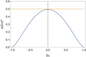
Figure 1: Plot of the variance of the position in the Lorentzian coherent state given by (4.23), where $\sigma/\lambda_{c}=8$. The dashed line corresponds to the value $0.5$ of the variance in the canonical coherent state (see (3.4)).

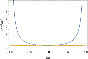
Figure 2: Variance of the momentum in the Lorentzian coherent state (4.34) given by (4.23) with $\sigma/\lambda_{c}=8$. The dashed line refers to the variance $0.5$ in the canonical coherent state (see (3.4)).

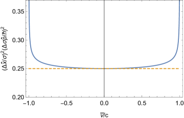
Figure 3: Plot of the product of variances of the position and momentum illustrated in Fig. 1 and Fig. 2. The dashed line corresponds to the value $0.25$ of the product in the canonical coherent state (see (3.4)).

5 Poincaré coherent states

5.1 Basic properties of the Poincaré coherent states

We now study the candidate for the relativistic coherent states introduced by Kaiser [43] and independently by Twareque Ali, Antoine and Gazeau [44, 45]. The special case of these states was discussed for the first time by Bakke and Wergeland [41, 42]. More precisely, the states considered by Bakke and Wergeland as packets that do not violate relativistic causality are of the form [42]

$$\tilde{\phi}(p)=C\frac{\exp(-\alpha\sqrt{p^{2}+m^{2}})}{(p^{2}+m^{2})^{\frac{1}{4}}},$$ (5.1)

where $\alpha$ is positive parameter, $C$ is a normalization constant, $\hbar=1$, $c=1$, and we assume that the Hilbert space is given by (3.8). We point out that the states (5.1) were not interpreted by Baake and Wergeland as the coherent ones. By virtue of (2.9) these states are equivalent in the one-dimensional counterpart of the Hilbert space (2.8) such that

$$\langle\phi^{\prime}|\psi^{\prime}\rangle=\frac{1}{\hbar}\int\frac{mc\,dp}{p^{0}(p)}{\tilde{\phi}}^{\prime*}(p){\tilde{\psi}}^{\prime}(p),$$ (5.2)

to the state

$$\tilde{\phi}^{\prime}(p)=C\exp(-\alpha\sqrt{p^{2}+m^{2}}).$$ (5.3)

The most general and systematic definition of the relativistic coherent states that can be regarded as a generalization of the states (5.3) was introduced by Twareque Ali, Antoine and Gazeau [44, 45]. Bearing in mind the denomination of these states utilized in [44, 45] we shall refer to them as the Poincaré coherent states. Based on the Perelomov approach [58] the above-mentioned coherent states are defined as

$$|q,k\rangle=U[\sigma_{\tau}(q,k)]|\psi_{0}\rangle,$$ (5.4)

where $U$ is an element of the unitary irreducible representation of the Poincaré group ${\cal P}^{\uparrow}_{+}(1,1)$ associated to elementary quantum system of mass $m>0$, $\sigma_{\tau}:\Gamma\to{\cal P}^{\uparrow}_{+}(1,1)$, is a section given by (B3) and $\Gamma={\cal P}^{\uparrow}_{+}(1,1)/T_{t}$, where $T_{t}$ is the subgroup of time translations, is the classical phase space with coordinates $(q,k)$. The fiducial vector $|\psi_{0}\rangle$ is referred to in [45] as a “probe”. On writing (5.4) in the momentum representation with invariant measure (5.2), we get the following formula for the coherent states

$$\tilde{\phi}^{\prime}_{(q,k)}(p)=U(\sigma_{\tau}(q,k))\psi_{0}(p)=\exp\left\{{\rm i}\left[\frac{k_{0}}{m}p_{0}\tau-\left(\frac{k}{m}p\tau+pq\right)\right]\right\}\psi_{0}(\Lambda_{k}^{-1}p),$$ (5.5)

where we set $\hbar=1$. Now, it is clear that in the discussed one-dimensional case the phase space should be parametrized solely by $q$ and $k$, so we set $\tau=0$. We remark that the section $\sigma_{0}(q,k)$ is called in [45] “Galilean” or “time zero” section. Furthermore, following [45] we put $\psi_{0}(p)=Ce^{-\frac{p_{0}}{\kappa}}$, where $C$ is a normalization constant and $\kappa$ is a constant with the dimension of energy. Hence, we finally get

$$\tilde{\phi}^{\prime}_{(q,k)}(p)=U(\sigma_{0}(q,k))Ce^{-\frac{p_{0}}{\kappa}}=C\exp\left(-\frac{1}{\kappa m}k_{0}p_{0}+\frac{1}{\kappa m}kp-{\rm i}pq\right),$$ (5.6)

where the normalization constant $C$ obtained by means of (5.2) and (4.21) is

$$C=\sqrt{\frac{\hbar}{2mcK_{0}\left(\frac{2mc^{2}}{\kappa}\right)}}.$$ (5.7)

The coherent states (5.6) can be written as

$$\tilde{\phi}^{\prime}_{(q,k)}(p)=Ce^{{\rm i}\underline{\hbox{$\scriptstyle p$}}\,\underline{\hbox{$\scriptstyle z$}}},$$ (5.8)

where $\underline{$p$}\,\underline{$z$}=p_{0}z_{0}-pz$, $\underline{$p$}$ is the four-momentum $\underline{$p$}=(p_{0},p)$ with $p_{0}(p)=\sqrt{p^{2}+m^{2}c^{2}}$, and $\underline{$z$}$ is the complex four-vector $\underline{$z$}=(z_{0},z)=\left({\rm i}\frac{k_{0}}{\kappa m},q+{\rm i}\frac{k}{\kappa m}\right)$.

We remark that it is straightforward to extend the construction of Poincaré coherent states described above to higher dimensions. The coherent states introduced by Kaiser [43] can be considered as such a generalization. More precisely, these states were defined in the Hilbert space with Lorentz invariant measure (5.2) as

$$\tilde{\phi}^{\prime}_{z}(p)=Ce^{{\rm i}\underline{\hbox{$\scriptstyle p$}}\,\underline{\hbox{$\scriptstyle z$}}},$$ (5.9)

where $\underline{$p$}\,\underline{$z$}=p_{0}z_{0}-{\bm{z}}\cdot{\bm{p}}$, $\underline{$p$}$ is the four-momentum: $\underline{$p$}=(p_{0},{\bm{p}})$, with $p_{0}({\bm{p}})=\sqrt{{\bm{p}}^{2}+m^{2}c^{2}}$, $\underline{$z$}$ is a complex four-vector such that $\underline{$z$}=(a_{0}+{\rm i}b_{0},{\bm{a}}+{\rm i}{\bm{b}})$, and $a_{0}$ is identified with $-ct$, so $\tilde{\phi}^{\prime}_{z}(p)$ are the time-dependend coherent states, where the dynamics is given by the Salpeter equation. The coherent state (5.9) has the finite norm only if $b_{0}^{2}-{\bm{b}}^{2}>0$, therefore we introduce the timelike four-vector $(b_{0},{\bm{b}})$ satisfying $b_{0}^{2}-{\bm{b}}^{2}=\eta^{2}$, where $\eta>0$. Hence, we obtain

$$\tilde{\phi}^{\prime}_{z}({\bm{p}})=C\exp[-\sqrt{{\bm{b}}^{2}+\eta^{2}}\sqrt{{\bm{p}}^{2}+m^{2}c^{2}}+{\bm{b}}\cdot{\bm{p}}+{\rm i}(-ct\sqrt{{\bm{p}}^{2}+m^{2}c^{2}}-{\bm{a}}\cdot{\bm{p}})].$$ (5.10)

We point out that the generalization of (5.9) was discussed in [43] referring to the case, when the vectors are elements of $n+1$-dimensional Minkowski space. Now, taking into account that the definition of coherent states should not depend on dynamics but a parametrization of a classical pase space, we set $t=0$. We also restrict for simplicity to the one dimensional case, so the Hilbert space of states is then given by (5.2). With these assumptions the coherent states (5.10) take the form

$$\tilde{\phi}^{\prime}_{z}(p)=C\exp(-\sqrt{b^{2}+\eta^{2}}\sqrt{p^{2}+m^{2}c^{2}}+bp-{\rm i}ap),$$ (5.11)

where the normalization constant $C$ obtained with the help of (5.2) and (4.21) is given by

$$C^{2}=\frac{\hbar}{2mcK_{0}(2mc\sqrt{b_{0}^{2}-b^{2}})}=\frac{\hbar}{2mcK_{0}(2mc\eta)}.$$ (5.12)

Comparing (5.6) and (5.7) with (5.11) and (5.12), respectively, we find that (5.6) and (5.11) represent the same coherent state. In the sequel we shall adopt parametrization of the coherent states utilized in (5.11).

We now analyze the physical meaning of the discussed coherent states. Using (5.2) we get the expectation value of the one-dimensional version of the Newton-Wigner (2.10) of the form

$${\hat{x}}_{\rm NW}={\rm i}\hbar\frac{\partial}{\partial p}-{\rm i}\frac{\hbar}{2}\frac{p}{p^{2}+m^{2}c^{2}},$$ (5.13)

in the coherent state (5.11). Namely, we have

$${\bar{x}}=a\hbar.$$ (5.14)

Furthermore, utilizing (5.2) and (4.15) we get the average value of the momentum in the Poincaré coherent state

$$\bar{p}=\frac{bmc}{\sqrt{b_{0}^{2}-b^{2}}}\frac{K_{1}(2mc\sqrt{b_{0}^{2}-b^{2}})}{K_{0}(2mc\sqrt{b_{0}^{2}-b^{2}})}=\frac{bmc}{\eta}\frac{K_{1}(2mc\eta)}{K_{0}(2mc\eta)}.$$ (5.15)

Taking into account the nonrelativistic limit of the Poincaré coherent states (compare (4.18)), we get

$$\qquad\eta=\frac{\sigma^{2}}{\lambda_{c}\hbar}.$$ (5.16)

Hence, we have

$$b=\frac{\sigma^{2}}{\hbar^{2}}\bar{p}\rho\left(\frac{\sigma}{\lambda_{c}}\right),\quad b_{0}=\sqrt{\eta^{2}+b^{2}}=\frac{\sigma^{2}}{\hbar^{2}}\sqrt{m^{2}c^{2}+{\bar{p}}^{2}\left[\rho\left(\frac{\sigma}{\lambda_{c}}\right)\right]^{2}},$$ (5.17)

where we set for brevity $\rho\left(\frac{\sigma}{\lambda_{c}}\right)=K_{0}\left[2\left(\frac{\sigma}{\lambda_{c}}\right)^{2}\right]/K_{1}\left[2\left(\frac{\sigma}{\lambda_{c}}\right)^{2}\right]$, and we finally obtain the Poincaré coherent states parametrized by the points of the classical phase space such that

$$\tilde{\phi}^{\prime}_{(\bar{x},\bar{p})}(p)= \sqrt{\frac{\hbar}{2mcK_{0}\left[2\left(\frac{\sigma}{\lambda_{c}}\right)^{2}\right]}}\exp\left(-\frac{\sigma^{2}}{\hbar^{2}}\sqrt{m^{2}c^{2}+{\bar{p}}^{2}\left[\rho\left(\frac{\sigma}{\lambda_{c}}\right)\right]^{2}}\sqrt{p^{2}+m^{2}c^{2}}\right.$$

$$\left.{}+\frac{\sigma^{2}}{\hbar^{2}}{\bar{p}}\rho\left(\frac{\sigma}{\lambda_{c}}\right)p-{\rm i}\frac{{\bar{x}}}{\hbar}p\right).$$ (5.18)

where $\tilde{\phi}^{\prime}_{(\bar{x},\bar{p})}(p)\equiv\tilde{\phi}^{\prime}_{(q(\bar{x},\bar{p}),k(\bar{x},\bar{p}))}(p)\equiv\tilde{\phi}^{\prime}_{z(\bar{x},\bar{p})}(p)$. We stress that neither the physical meaning of the invariant $\eta$ nor the parametrization of the coherent states by points of the classical phase space were discussed in [43]. We point out that for $\bar{p}=0$ and ${\bar{x}}=0$ the states (5.18) reduce to the wave functions (5.3) introduced by Bakke and Wergeland. We also remark that in opposition to the canonical coherent states and the Lorentzian ones, the Poincaré coherent states are not marked by a complex number parametrizing the points of the classical phase space $(\bar{x},\bar{p})$. Furthermore, the reason is unclear for calling the states (5.18) the coherent ones. For instance their interpretation is dim as the states closest to the classical ones.

5.2 Position-momentum uncertainty relations in the Poincaré coherent states

We now discuss the Heisenberg position-momentum uncertainty relations in the Poincaré coherent states. The variance of the position obtained with the use of the completeness of the momentum eigenvectors $|p\rangle$ spanning the representation (5.2) can be written as

$$(\Delta{\hat{x}}_{\rm NW})^{2}=\overline{({\hat{x}}_{\rm NW}-{\bar{x}})^{2}}=\frac{\hbar^{2}}{2K_{0}\left[2\left(\frac{\sigma}{\lambda_{c}}\right)^{2}\right]}\int\frac{dp}{\sqrt{p^{2}+m^{2}c^{2}}}$$

$$\times\left(-\frac{\sigma^{2}}{\hbar^{2}}\sqrt{m^{2}c^{2}+{\bar{p}}^{2}\left[\rho\left(\frac{\sigma}{\lambda_{c}}\right)\right]^{2}}\frac{p}{\sqrt{p^{2}+m^{2}c^{2}}}+\frac{\sigma^{2}}{\hbar^{2}}{\bar{p}}\rho\left(\frac{\sigma}{\lambda_{c}}\right)-\frac{1}{2}\frac{p}{p^{2}+m^{2}c^{2}}\right)^{2}$$

$$\times\exp\left(-2\frac{\sigma^{2}}{\hbar^{2}}\sqrt{m^{2}c^{2}+{\bar{p}}^{2}\left[\rho\left(\frac{\sigma}{\lambda_{c}}\right)\right]^{2}}\sqrt{p^{2}+m^{2}c^{2}}+2\frac{\sigma^{2}}{\hbar^{2}}{\bar{p}}\rho\left(\frac{\sigma}{\lambda_{c}}\right)p\right).$$ (5.19)

We do not know any other formula for the variance simpler than the integral (5.19). Using (4.21) and elementary properties of the Bessel functions we find after some calculation

$$(\Delta\hat{p})^{2}=\frac{1}{2}\frac{\hbar^{2}}{\sigma^{2}}\frac{1}{\rho\left(\frac{\sigma}{\lambda_{c}}\right)}+{\bar{p}}^{2}\left\{\rho\left(\frac{\sigma}{\lambda_{c}}\right)\frac{K_{2}\left[2\left(\frac{\sigma}{\lambda_{c}}\right)^{2}\right]}{K_{1}\left[2\left(\frac{\sigma}{\lambda_{c}}\right)^{2}\right]}-1\right\}.$$ (5.20)

The dimensionless variances $(\Delta{\hat{x}}_{\rm NW}/\sigma)^{2}$, $(\Delta\sigma{\hat{p}}/\hbar)^{2}$, and their product are depicted in Fig. 4,5 and 6, respectively. As with the case of the Lorentzian coherent states we deal with better localization accuracy of position observable in comparison with the canonical coherent states and increasing of the variance of the momentum observable. Nevertheless, in opposition to the Lorentzian coherent states for the Poincaré ones we have plateau on the plot of the product of variances of the position and momentum observables.

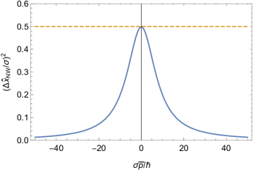
Figure 4: Variance of the position in the Poincaré coherent state (5.18) specified by (5.19) with $\sigma/\lambda_{c}=8$. The dashed line corresponds to the value $0.5$ of the variance in the canonical coherent state (see (3.4)).

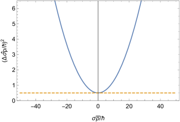
Figure 5: Plot of the variance of the momentum in the Poincaré coherent state (5.18) given by (5.20), where $\sigma/\lambda_{c}=8$. The dashed line refers to the variance $0.5$ in the canonical coherent state (see (3.4)).

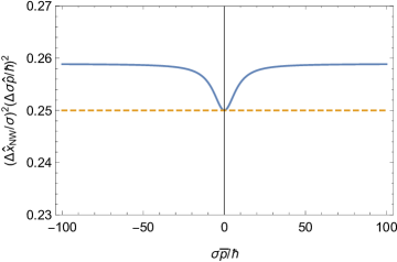
Figure 6: The product of variances of the position and momentum illustrated in Fig. 4 and Fig. 5. The dashed line corresponds to the value $0.25$ of the product in the canonical coherent state (see (3.4)).

The Poincaré coherent states are not orthogonal. On making use of the completeness of eigenvectors $|p\rangle$ of the momentum operator we arrive at the following formula for the overlapping integral

$$\langle\bar{x},\bar{p}|{\bar{x}}^{\prime},{\bar{p}}^{\prime}\rangle=\frac{1}{K_{0}\left[2\left(\frac{\sigma}{\lambda_{c}}\right)^{2}\right]}K_{0}\left\{mc\left[\left(\frac{\sigma}{\hbar}\right)^{4}\left(\sqrt{m^{2}c^{2}+{\bar{p}}^{2}\left[\rho\left(\frac{\sigma}{\lambda_{c}}\right)\right]^{2}}\right.\right.\right.$$

$$\left.\left.\left.{}+\sqrt{m^{2}c^{2}+{\bar{p}}^{\prime 2}\left[\rho\left(\frac{\sigma}{\lambda_{c}}\right)\right]^{2}}\right)^{2}-\left(\frac{\sigma^{2}}{\hbar^{2}}\rho\left(\frac{\sigma}{\lambda_{c}}\right)({\bar{p}}+{\bar{p}}^{\prime})+{\rm i}\frac{{\bar{x}}-{\bar{x}}^{\prime}}{\hbar}\right)^{2}\right]^{\frac{1}{2}}\right\},$$ (5.21)

where $\tilde{\phi}^{\prime}_{z}(p)\equiv\langle p|{\bar{x}},{\bar{p}}\rangle$. The Poincaré coherent states form a complete set. Indeed, using the orthogonality condition satisfied by the momentum eigenvectors spanning the basis of the representation (5.2) such that

$$\langle p|p^{\prime}\rangle=\frac{\hbar}{mc}\sqrt{p^{2}+m^{2}c^{2}}\delta(p-p^{\prime}),$$ (5.22)

we get the resolution of the identity for the Poincaré coherent states of the form

$$\frac{1}{2\pi\hbar}\left[\rho\left(\frac{\sigma}{\lambda_{c}}\right)\right]^{2}\int d{\bar{x}}d\bar{p}\,|\bar{x},\bar{p}\rangle\langle{\bar{x}},\bar{p}|=I.$$ (5.23)

It thus appears that up to multiplicative constant the resolution of the identity for the Poincaré coherent states has the same form as in the case of the canonical states (see (3.7)).

5.3 Expectations of relativistic observables in the Poincaré coherent states

We now investigate the behavior of relativistic observables in the Poincaré coherent states that can be regarded as a measure of the closeness of these states to the classical phase space. Taking into account (4.15) we derive the following formula for the expectation value of the energy

$$\bar{E}=\overline{\sqrt{{\hat{p}}^{2}c^{2}+m^{2}c^{2}}}=\sqrt{{\bar{p}}^{2}c^{2}+\left[\frac{mc^{2}}{\rho\left(\frac{\sigma}{\lambda_{c}}\right)}\right]^{2}}.$$ (5.24)

Notice that as with the Lorentzian coherent states, the average energy and momentum do not satisfy the relativistic dispersion relation. We also remark that

$$\frac{1}{c}\sqrt{\left(\frac{{\bar{E}}}{c}\right)^{2}-{\bar{p}}^{2}}=\frac{m}{\rho\left(\frac{\sigma}{\lambda_{c}}\right)}=m\frac{K_{1}\left[2\left(\frac{\sigma}{\lambda_{c}}\right)^{2}\right]}{K_{0}\left[2\left(\frac{\sigma}{\lambda_{c}}\right)^{2}\right]},$$ (5.25)

was interpreted in [43] as the “effective” mass of a particle, with the parameter $K_{1}\left[2\left(\frac{\sigma}{\lambda_{c}}\right)^{2}\right]/K_{0}\left[2\left(\frac{\sigma}{\lambda_{c}}\right)^{2}\right]$ playing the role of a renormalization which takes into effect the fluctuation in energy-momentum. Furthermore, the average velocity in the Poincaré coherent state that can be easily obtained with the help of (4.15) is given by

$$\bar{v}=\overline{\left(\frac{c\hat{p}}{\sqrt{{\hat{p}}^{2}+m^{2}c^{2}}}\right)}=\frac{2\left(\frac{\sigma}{\lambda_{c}}\right)^{2}\frac{\bar{p}}{m}}{K_{1}\left[2\left(\frac{\sigma}{\lambda_{c}}\right)^{2}\right]}\int_{\frac{\sigma^{2}}{\lambda_{c}\hbar}}^{\infty}\frac{K_{1}(2mcu)}{\sqrt{u^{2}+\left(\frac{\sigma}{\hbar}\right)^{4}{\bar{p}}^{2}\left[\rho\left(\frac{\sigma}{\lambda_{c}}\right)\right]^{2}}}du.$$ (5.26)

Numerical calculations show that for $\sigma/\lambda_{c}\geqslant 5$ and $\sigma/\lambda_{c}\geqslant 8$ we have the approximate relations of the form (3.19) and (3.31), repectively, so the behavior of expectation values of energy and velocity in the Poincaré coherent states is the same as in the case of the canonical ones.

6 Conclusions

In this work we discuss the three approaches to relativistic coherent states of a spinless particle: the canonical coherent states, Lorentzian and Poincaré ones. An advantage of the canonical coherent states is saturation of the Heisenberg uncertainty relations and possibility of their application in the case of the massless particles. Furthermore, the behavior of expectation values of quantum observables in these states is as good or better than for the remaining candidates. The problems are connected with the Lorentz covariance of the canonical coherent states. An asset of the Lorentzian coherent states is the minimization of uncertainty relations involving position and relativistic velocity and analytic form of averages of observables expressed in terms of the Bessel functions that are ubiquitous in relativistic quantum theory. Furthermore, these states can be obtained by means of the Thiemann complexifier method that has already proven its generality in the case of the canonical coherent states and coherent states for a particle on a circle and sphere [59]. The problematic issue are position-momentum uncertainty relations. More precisely, the behavior of the variance of the momentum observable and product of variances of position and momentum operators that is unusual for coherent states. Another problem is the completeness of the Lorentzian coherent states. Indeed, the formula for the resolution of the identity for these states should involve integral identities satisfied by the Bessel functions on the interval $(-1,1)$. The authors have not found such identities in the literature. Finally, it is not clear why in the relativistic quantum mechanics the coherent states would be parametrized by average position $\bar{x}$ and velocity $\bar{v}$ instead of the point of the classical phase space $(\bar{x},\bar{p})$ as in the nonrelativistic case. An advantage of the Poincaré coherent states is their Lorentz covariance. Furthermore, the plateau on the plot of the product of variances of position and momentum variables resembles the behavior of canonical coherent states. The parametrization of the Poincaré coherent states by means of the Bessel functions seems to be also plausible in relativistic quantum mechanics. As with the canonical coherent states these states are parametrized by points $(\bar{x},\bar{p})$ of the classical phase space. We have also similar resolution of the identity. On the other hand, the behavior is problematic of the variance of the momentum observable analogous to that in the Lorentzian coherent states. In the light of the above comments, there is no convincing evidence which candidate for the relativistic coherent states is better.

Appendix A Confluent hypergeometric function

We first recall some properties of the confluent hypergeometric function $U(a,b,z)$. This function can be expressed by means of the hypergeometric function ${}_{1}F_{1}(a,b;z)$. Namely,

$$U(a,b,z)=\frac{\Gamma(1-b)}{\Gamma(a+1-b)}{}_{1}F_{1}(a,b;z)+\frac{\Gamma(b-1)}{\Gamma(a)}z^{1-b}{}_{1}F_{1}(a+1-b,2-b;z).$$ (A.1)

The confluent hypergeometric function satisfies the following relations

$$U(a,b,z) =z^{1-b}U(a-b+1,2-b,z),$$ (A.2)

$$\frac{d^{n}}{dz^{n}}[z^{b-1}U(a,b,z)] =(-1)^{n}(a-b+1)_{n}z^{b-n-1}U(a,b-n,z),$$ (A.3)

where $(\alpha)_{n}$ is the Pochhammer’s symbol $(\alpha)_{n}=\alpha(\alpha+1)\ldots(\alpha+n-1)$ and $(\alpha)_{0}=1$. We have also the recurrence relation fulfilled by this function such that

$$U(a,b,z)-aU(a+1,b,z)-U(a,b-1,z)=0.$$ (A.4)

Appendix B Generation of the Poincaré coherent states

We now discuss the details of the generation of the Poincaré coherent states described by the formula (5.4). In order to make the formalism introduced in [8] more transparent we use the following representation of the Poincaré group ${\cal P}^{\uparrow}_{+}(1,1)$ element $g(\Lambda,\underline{a})$ with $\underline{a}=\left(\begin{smallmatrix}a^{0}\\ a^{1}\end{smallmatrix}\right)$:

$$g(\Lambda,\underline{a})=\begin{pmatrix}\hphantom{0}\Lambda\hphantom{0}&\underline{a}\\ 0\hphantom{0}0&1\end{pmatrix}$$ (B.1)

Furthermore, the parametrization of the phase space $\Gamma={\cal P}^{\uparrow}_{+}(1,1)/T_{t}$ utilizes the following factorization of the element $g(\Lambda_{k},\underline{x})$, where $\Lambda_{k}=\frac{1}{m}\left(\begin{smallmatrix}k^{0}&k\\ k&k^{0}\end{smallmatrix}\right)$ is the Lorentz boost matrix and $\underline{x}=\left(\begin{smallmatrix}t\\ x\end{smallmatrix}\right)$:

$$g(\Lambda_{k},\underline{x})=\begin{pmatrix}\hphantom{0}\Lambda_{k}\hphantom{0}&\underline{x}\\ 0\hphantom{0}0&1\end{pmatrix}=\begin{pmatrix}\hphantom{0}\Lambda_{k}\hphantom{0}&\begin{pmatrix}0\\ q\end{pmatrix}\\ 0\hphantom{0}0&1\end{pmatrix}\begin{pmatrix}\hphantom{0}I\hphantom{0}&\begin{pmatrix}\tau\\ 0\end{pmatrix}\\ 0\hphantom{0}0&1\end{pmatrix}$$ (B.2)

which leads to the section of the form

$$\sigma_{\tau}(q,k)=\begin{pmatrix}\hphantom{0}\Lambda_{k}\hphantom{0}&\frac{1}{m}\begin{pmatrix}\tau k^{0}\\ \tau k+mq\end{pmatrix}\\ 0\hphantom{0}0&1\end{pmatrix}.$$ (B.3)

References

- [1] E. Schrödinger, Ann. Phys. 81 (1926) 109.
- [2] O. Klein, Z. Phys. 37 (1926) 895.
- [3] V.A. Fock, Z. Phys. 38 (1926) 242; V.A. Fock, Z. Phys. 39 (1926) 226.
- [4] W. Gordon, Z. Phys. 40 (1926) 117; W. Gordon, Z. Phys. 40 (1926) 121.
- [5] E.E. Salpeter, Phys. Rev. 87 (1952) 328.
- [6] L.L. Foldy, Phys. Rev. 102 (1956) 568.
- [7] G. Paiano, Nuovo Cimento 70 (1982) 339.
- [8] P. Cea, P. Calangelo, G. Nardulli, G. Paiano and G. Preparata, Phys. Rev. D 26 (1982) 1157.
- [9] P. Cea, G. Nardulli and G. Paiano, Phys. Rev. D 28 (1983) 2291.
- [10] L.M. Nickisch and L. Durand, Phys. Rev D 30 (1984) 660.
- [11] J.B. Rosenstein and L.P. Horwitz, J. Phys. A 18 (1985) 2115.
- [12] C. Lämmerzahl, J. Math. Phys. 34 (1993) 3918.
- [13] W. Lucha and F.F. Schöberl, Phys. Rev. D 50 (1994) 5443.
- [14] F. Brau, J. Math. Phys. 39, 2254 (1998).
- [15] R.L. Hall, W. Lucha and F.F. Schöberl, J. Phys. A 34 (2001) 5059.
- [16] R.L. Hall, W. Lucha and F.F. Schöberl, J. Math. Phys. 42 (2001) 5228.
- [17] R.L. Hall, W. Lucha and F.F. Schöberl, J. Math. Phys.43 (2002) 5913.
- [18] R.L. Hall, W. Lucha and F.F. Schöberl, Int. J. Mod. Phys. A 18 (2003) 2657.
- [19] F. Brau, Phys. Lett. A 313 (2003) 363.
- [20] Zhi-Feng Li, Jin-Jin Liu, W. Lucha and F.F. Schöberl, J. Math. Phys. 46 (2005) 103514.
- [21] R.L. Hall and W. Lucha, J. Phys. A 38 (2005) 7997.
- [22] Y. Chargui, L. Chetouani and A. Trabelsi, J. Phys. A: Math. Theor. 42 (2009) 355203.
- [23] K. Kowalski and J. Rembieliński, Phys. Rev. A 81 (2010) 012118.
- [24] D. Babusci, G. Dattoli and M. Quattromini, Phus. Rev. A 83 (2011) 062109.
- [25] K. Kowalski and J. Rembieliński, Phys. Rev. A 84 (2011) 012108.
- [26] P. Garbaczewski and V. Stephanovich, J. Math. Phys. 54 (2013) 072103.
- [27] M. Żaba and P. Garbaczewski, J. Math. Phys. 55 (2014) 092103.
- [28] G. Dattoli, E. Sabia, K. Górska, A. Horzela and K. A. Penson, J. Phys. A: Math. Theor. 48 (2015) 125203.
- [29] F. Gross, Relativistic Quantum Mechanics and Field Theory, Wiley, Weinheim, 1993.
- [30] J. Dimock, Quantum Mechanics and Quantum Field Theory. A Mathematical Primer, Cambridge University Press, Cambridge, 2011.
- [31] K. Kowalski and J. Rembieliński, Ann. Phys. 375 (2016) 1.
- [32] O.I. Zavialov and A.M. Malokostov, Theor. Math. Phys. 119 (1999) 448.
- [33] L.J. Nickisch and L. Durand, Phys. Rev. D 30 (1984) 660.
- [34] J.L. Basdevant and S. Boukraa, Z. Phys. C 28 (1985) 413.
- [35] I.A. Malkin and V.I. Man’ko, Sov. Phys. JETP 28 (1969) 527.
- [36] B.I. Lev, A.A. Semenov, C.V. Usenko and J.R. Klauder, Phys. Rev. A 66 (2002) 022115.
- [37] B.I. Lev, A.A. Semenov and C.V. Usenko, Phys. Lett. A 230 (1997) 261.
- [38] V.G. Bagrov, I.L. Buchbinder and D.M. Gitman, J. Phys. A: Math. Gen. 9 (1976) 1955.
- [39] H. Feshbach and F. Villars, Rev. Mod. Phys. 30 (1958) 24.
- [40] A. Mostafazadeh and F. Zamani, Ann. Phys. 321 (2006) 2210.
- [41] F. Baake and H. Wergeland, Physica 69 (1973) 5.
- [42] C. Almeida, Am. J. Phys. 52 (1984) 921.
- [43] G. Kaiser, J. Math. Phys. 18 (1977) 952.
- [44] S. Twareque Ali and J.-P. Antoine, Ann. Inst. H. Poincaré 51 (1989) 23.
- [45] S. Twareque Ali, J.-P. Antoine and J.-P. Gazeau, Ann. Phys. 222 (1993) 38.
- [46] K. Kowalski, J. Rembieliński and L.C. Papaloucas, J. Phys. A 29 (1996) 4149.
- [47] K. Kowalski and J. Rembieliński, J. Phys. A 33 (2000) 6035.
- [48] K. Kowalski and J. Rembieliński, Phys. Rev A 75 (2007) 052102.
- [49] K. Kowalski and J. Rembieliński, J. Phys. A: Math. Theor. 41 (2008) 304021.
- [50] F.W.J. Olver (Ed.), NIST Handbook of Mathematical Functions, Cambridge University Press, Cambridge, 2010.
- [51] I.S. Gradshteyn and I.M. Ryzhik, Tables of Integrals, Series, and Products, Elsevier, Amsterdam, 2007.
- [52] B. Rosenstein and M. Usher, Phys. Rev. D 36 (1987) 2381.
- [53] B. Rosenstein and L.P. Horwitz, J. Phys. A 18 (1985) 2115.
- [54] F.W. Strauch, Phys. Rev. A 73 (2006) 054302.
- [55] M.H. Al-Hashimi and U.-J. Wiese, Ann. Phys. 324 (2009) 2599.
- [56] T. Thiemann, Classical Quantum Gravity 13 (1996) 1383.
- [57] A.P. Prudnikov, Yu. A. Brychkov and O.I. Marichev, Integrals and Series. Vol 1. Elementary functions, Fizmatlig, Moscow, 2002.
- [58] A. Perelomov, Generalized Coherent States and Their Applications, Springer, Berlin, 1986.
- [59] K. Kowalski and J. Rembieliński, J. Math. Phys. 42 (2001) 4138.