Measurement-induced non-locality in arbitrary dimensions in terms of the inverse approximate joint diagonalization

Abstract

The computability of the quantifier of a given quantum resource is the essential challenge in the resource theory and the inevitable bottleneck for its application. Here we focus on the measurement-induced non-locality and present a new definition in terms of the skew information subject to a broken observable. It is shown that the new quantity possesses an obvious operational meaning, can tackle the non-contractivity of the measurement-induced non-locality and has an analytic expressions for pure states, ($2\otimes d$)-dimensional quantum states and some particular high-dimensional quantum states. Most importantly, an inverse approximate joint diagonalization algorithm, due to its simplicity, high efficiency, stability and state independence, is presented to provide the almost analytic expressions for any quantum state, which can also shed new light on the other aspects in physics. As applications as well as the demonstration of the validity of the algorithm, we compare the analytic and the numerical expressions of various examples and show the perfect consistency.

I Introduction

Quantum mechanical phenomena such as entanglement are not only fundamental properties of quantum mechanics, but also the important physical resources due to their exploitation in quantum information processing tasks. Thus a mathematical quantitative theory, i.e., the resource theory (RT), is required to characterize the resource feature of these quantum phenomena. In the recent years, the RT has been deeply developed for entanglement B1 ; B2 ; B3 ; o1 ; o2 ; o3 , quantum discord d1 ; d2 ; d3 ; d4 ; d5 ; d6 and quantum coherence c1 ; c2 ; c3 ; c4 ; c5 ; c6 and so on t1 ; t2 . However, as the core in RT, a good measure for the given resource of a general (especially high-dimensional) quantum state is only available for quantum coherence c1 ; yuc . In contrast, quantum entanglement and quantum discord can be only well quantified in quite limited states peres ; wootters ; vidal ; geom1 ; geom ; dak ; giro ; diagon . Undoubtedly, their common challenge is the computability of the given measure (despite that some conceptual question, e.g., the entanglement measure of multipartite states etc., remains open). In order to study these quantum features, especially entanglement in a general (high-dimensional) quantum system, people usually have to seek for the lower or upper bounds for the rough reference o2 ; florian ; kai ; ycc . Comparably, an effective numerical way to evaluating a measure could be even more important for its potential applications in both the measure itself and the large-scale quantum system. For example, the conjugate-gradient method was proposed to calculate the bipartite entanglement of formation nc ; the semi-definite programming method was used to find the best separable approximation semi ; some numerical algorithms were developed for the evaluation of the relative-entropy entanglement of bipartite states nr ; nume ; compu ; 3-tangle can also be evaluated by various numerical ways such as the Monto Carlo methods nm , the conjugate-gradient method and so on compu ; highly ; numerical ; the local quantum uncertainty can be stably computed based on the approximate joint diagonalization algorithm diagon ; recently, the numerical algorithms have also been used to calculate the quantum coherence measures robu ; asym ; trac ; gene . Generally speaking, a numerical algorithm depends not only on the question (the measure) but also on the state to be evaluated. In this sense, how to develop an effective algorithm for a particular quantum resource especially independent of the state is still of great practical significance.

In this paper, we present an effective numerical algorithm for the measurement-induced non-locality loca . the measurement-induced non-locality, dual to the quantum discord (to some extent) d1 ; d2 , is one type of non-locality that characterizes the global disturbance on a composite state caused by the local non-disturbing measurement on one subsystem. However, the measurement-induced non-locality, similar to the geometric quantum discord dak ; geometr , is originally defined based on the $l_{2}$ norm and inherits its non-contractivity, so it is not a good measure due to the some unphysical phenomena that could be induced piani . Although the measurement-induced non-locality has been studied in many aspects SY ; gamy ; Rana ; Wu ; Hu ; maximal ; based , no obvious operational meaning has been found up to now and in particular, it can only be analytically calculated in low-dimensional quantum systems loca ; Wu ; Hu . Here we will first redefine the measurement-induced non-locality based on the skew information skew ; convex ; uncer in terms of the broken observable (a complete set of rank-one projectors) instead of a single observable. Thus not only the non-contractivity can be automatically solved, but also an obvious operational meaning related to quantum metrology has been found. Another distinct advantage of such a re-definition is that it can be analytically calculated for a large class of high-dimensional states and especially can induce a powerful numerical means, i.e., the inverse approximate joint diagonalization, to find the almost analytic expression for any quantum state. It is shown that this algorithm can be stably and simply performed with even the machine precision and especially it is state independent. The effectiveness of the algorithm is demonstrated by comparison with the analytic results of various examples. The remaining of this paper is organized as follows. In Sec. II, we briefly introduce the measurement-induced non-locality and present its new definition as well as its operational meaning. In Sec. III, we detailedly introduce the inverse approximate joint diagonalization algorithm and show how we convert the measurement-induced non-locality to the standard optimization question governed by the the inverse approximate joint diagonalization. In Sec. IV, we demonstrate the power of the new definition and the algorithm by various applications. The conclusion is obtained in Sec. V.

II The measurement-induced non-locality based on the skew information

The definition.-To begin with, we briefly introduce the measurement-induced non-locality loca based on the $l_{2}$ norm. For a bipartite density matrix $\rho_{AB}$, the measurement-induced non-locality is defined by the maximal disturbance of local projective measurements as

$$N(\rho_{AB})=\max_{\Pi}\left\|\rho-\Pi^{A}(\rho_{AB})\right\|_{2}^{2},$$ (1)

where $\left\|\cdot\right\|_{2}$ denotes the $l_{2}$ norm of a matrix, the von Neumann measurement $\Pi^{A}$ is defined by $\sum_{k}(\Pi_{k}^{A}\otimes\mathbb{I}^{B})\rho_{AB}(\Pi_{k}^{A}\otimes\mathbb{I}^{B})$ with $\sum_{k}\Pi_{k}^{A}\rho_{A}\Pi_{k}^{A}=\rho_{A}$ guaranteeing that the reduced density matrix $\rho_{A}=\mathrm{Tr}_{B}\rho_{AB}$ is not disturbed. The measurement-induced non-locality can be analytically calculated for two-qubit systems, but it is not contractive in that the measurement-induced non-locality can be increased by some local operations on subsystem B and decreased by the tensor product of a third independent subsystem. In order to avoid the non-contractivity, we can effectively utilize the properties of the skew information and directly present our definition of the measurement-induced non-locality in the following rigorous way.

Definition 1.- For an ($m\otimes n$)-dimensional density $\rho_{AB}$, the measurement-induced non-locality can be defined in terms of skew information as

$$U(\rho_{AB})=\max_{\left\{K_{k}\right\}}\sum_{k=0}^{m-1}I\left(\rho_{AB},K_{k}\right),$$ (2)

where $I\left(\rho_{AB},K_{k}\right)=-\frac{1}{2}\mathrm{Tr}[\sqrt{\rho_{AB}},K_{k}]^{2}$ is the quantum skew information and $K_{k}=\left|k\right\rangle_{A}\left\langle k\right|\otimes\mathbb{I}_{B}$ with $\left|k\right\rangle$ denoting the eigenvectors of the reduced density matrix $\rho_{A}$.

At first, one can find that (i) $U(\rho_{AB})=0$ for any product state $\rho_{AB}=\rho_{A}\otimes\rho_{B}$; (ii) $U(\rho_{AB})$ is invariant under local unitary transformations; (iii) $\rho_{AB}$ vanishes for any classical-quantum state $\rho_{AB}=\sum_{k}p_{k}\left|k\right\rangle_{A}\left\langle k\right|\otimes\rho_{B}$ with the nondegenerate reduced density matrix $\rho_{A}$; (iv) $U(\rho_{AB})$ is equivalent to the entanglement for pure $\rho_{AB}$, which can be found from our latter Eq. (22). All the above properties of our redefined $U(\rho_{AB})$ are completely the same as the fundamental properties of the measurement-induced non-locality given in Ref. loca . This means that our $U(\rho_{AB})$ characterizes the same quantum resource as that in Ref. loca . In addition, it is obvious that $U(\rho_{AB})$ is contractive and it is invariant under local unitary operations as a result of the good properties of the skew information. In addition, it can be found that the above definition of measurement-induced non-locality has the obvious operational meaning related to quantum metrology.

Operational meaning.- Let’s consider a scheme of quantum metrology as follows. Suppose we have an $(m\otimes n)$-dimensional state $\rho_{AB}$ with the reduced density matrix $\rho_{A}$ and then let the state undergo a unitary operation $U_{\varphi_{k}}=e^{-iK_{k}\varphi_{k}}$ with $K_{k}=\left|k\right\rangle_{A}\left\langle k\right|\otimes\mathbb{I}_{B}$ and $\left[\left|k\right\rangle\left\langle k\right|,\rho_{A}\right]=0$. This will endow an unknown phase $\varphi_{k}$ to the state $\rho_{AB}$ as $\rho_{k}=U_{\varphi_{k}}\rho_{AB}U_{\varphi_{k}}^{\dagger}$. We aim to estimate the measurement precision by measuring $\varphi_{k}$ in $\rho_{k}$ with $N>>1$ runs of detection on $\rho_{k}$.

In the above scheme, the measurement precision of $\varphi_{k}$ is characterized by the uncertainty of the estimated phase $\varphi_{k}^{est}$ defined by

$$\delta\varphi_{k}=\left\langle\left(\frac{\varphi_{k}^{est}}{\left|\partial\left\langle\varphi_{k}^{est}\right\rangle/\partial\varphi_{k}\right|}-\varphi_{k}\right)^{2}\right\rangle^{1/2}$$ (3)

which, for an unbiased estimator, is just the standard deviation fis2 ; fis1 ; fis11 . Based on the quantum parameter estimationfis2 ; fis1 ; fis11 , $\delta\varphi_{k}$ is limited by the quantum Cramér-Rao bound as $\left(\delta\varphi_{k}\right)^{2}\geq\frac{1}{NF_{Qk}}$, where $F_{Qk}=\mathrm{Tr}\{\rho_{\varphi}L_{\varphi}^{2}\}$ is the quantum Fisher information with $L_{\varphi}$ being the symmetric logarithmic derivative defined by $2\partial_{\varphi}\rho_{\varphi}=L_{\varphi}\rho_{\varphi}+\rho_{\varphi}L_{\varphi}$ fis2 . It was shown in Refs. fis2 ; fis1 ; fis11 that this bound can always be reached asymptotically by maximum likelihood estimation and a projective measurement in the eigen-basis of the ”symmetric logarithmic derivative operator” . Thus one can let $\left(\delta\varphi_{k}^{o}\right)^{2}$ to denote the optimal variance which achieves the Cramér-Rao bound, i.e., $\left(\delta\varphi_{k}^{o}\right)^{2}=\frac{1}{NF_{Qk}}$. Ref. luo1 showed that the Fisher information $F_{Qk}$ is well bounded by the skew information as

$$\frac{F_{Qk}}{4}\leq 2I\left(\rho_{AB},K_{k}\right)\iff\frac{1}{\left(\delta\varphi_{k}^{o}\right)^{2}}\leq 8NI(\rho_{AB},K_{k}).$$ (4)

Suppose we repeat this scheme $N$ times respectively corresponding to a complete set $\{\left.K_{k}\right|\left[\left|k\right\rangle\left\langle k\right|,\rho_{A}\right]=0\}$, we can sum Eq. (4) over $k$ as

$$\sum_{k}\frac{1}{\left(\delta\varphi_{k}^{o}\right)^{2}}\leq 8N\sum_{k}I(\rho_{AB},K_{k})\leq 8NU(\rho_{AB}),$$ (5)

where the last inequality comes from Eq. (2). If we define $\frac{1}{(\Delta_{\varphi}^{o})^{2}}=\sum_{k}\frac{1}{\left(\delta\varphi_{k}^{o}\right)^{2}}$, Eq. (5) can be rewritten as

$$\frac{1}{8NU(\rho_{AB})}\leq(\Delta_{\varphi}^{o})^{2},$$ (6)

which shows that the measurement-induced non-locality $U(\rho_{AB})$ contributes to the lower bounds of the “average variance” $(\Delta_{\varphi}^{o})^{2}$ that characterizes the contributions of all the inverse optimal variances of the estimated phases. It is worth emphasizing that $(\Delta_{\varphi}^{o})^{2}$ corresponds to an arbitrary complete set $\{\left.K_{k}\right|\left[\left|k\right\rangle\left\langle k\right|,\rho_{A}\right]=0\}$ instead of the optimal set in the sense of Eq. (2). In addition, in the above mentioned asymptotical and the optimal regimes, Eq. (6) for the pure states will become $\frac{1}{4NU(\rho_{AB})}=(\Delta_{\varphi}^{o})^{2}$ due to the inequality $\frac{F_{Qk}}{4}\geq I\left(\rho_{AB}\right)$ luo1 . However, one can recognize that in the practical scenario, $\delta\varphi_{k}\geq\delta\varphi^{o}_{k}$ because the measurement protocol couldn’t be optimal. Thus, one can immediately obtain

$$\sum_{k}\frac{1}{\left(\delta\varphi_{k}\right)^{2}}\leq 8NU\left(\rho_{AB}\right)\iff\frac{1}{8NU(\rho_{AB})}\leq(\Delta_{\varphi})^{2},$$ (7)

with $\frac{1}{(\Delta_{\varphi})^{2}}=\sum_{k}\frac{1}{\left(\delta\varphi_{k}\right)^{2}}$. Thus we would like to emphasize that Eq. (7) and Eq. (6) provide only the lower bound instead of the exact value of the “average variance” $(\Delta_{\varphi})^{2}$ or $(\Delta_{\varphi}^{o})^{2}$, because the inequalities are not saturated in the general cases. In this sense, our measurement-induced non-locality was endowed with the operational meaning.

III The effective numerical algorithm and the measurement-induced non-locality in arbitrary dimension

The approximate joint diagonalization algorithm.- In order to give our main inverse approximate joint diagonalization algorithm, we first introduce the well-known approximate joint diagonalization algorithm blind ; jacibo ; fast and its relevant approximate joint diagonalization optimization problem. For $m$ n-dimensional matrices $\{M_{m}\}$, one aims to find a unitary matrix $U$ such that

$$J(U)=\max_{U}\sum_{i=1}^{m}\sum_{k=1}^{n}|UM_{i}U^{\dagger}|_{kk}^{2}.$$ (8)

Such an optimization problem is a standard expression of the approximate joint diagonalizationapproximate joint diagonalization of the series of matrices $M_{i}$. This approximate joint diagonalization problem is widely met in the Blind Source Separation and Independent Component Analysis (See Ref. golub and the references therein) and is well solved numerically by many effective algorithms . A very remarkable algorithm is the Jocabi method blind ; jacibo ; golub which can be performed as steadily, reliably, fast and perfectly as the diagonalization of a single matrix. The main idea of the approximate joint diagonalization algorithm of our interest is as follows.

Any unitary matrix $U$ can be decomposed into a series of unitary matrices called Givens rotations as $U=\Pi_{\{\theta,\phi\}}U(\theta,\phi)$ with

$$U(\theta,\phi)=\begin{pmatrix}\cos\theta&e^{i\varphi}\sin\theta\\ -e^{-i\varphi}\sin\theta&\cos\theta\end{pmatrix}.$$ (9)

Each Givens rotation is only operated on the $(2\times 2)$-dimensional subspace of the $m$ $M_{i}$’s. Let

$$G_{i}=\begin{pmatrix}a_{i}&b_{i}\\ c_{i}&d_{i}\end{pmatrix}$$ (10)

denote the $(2\times 2)$-dimensional block matrix of $M_{i}$ corresponding to the Givens rotation $U(\theta,\phi)$. After the Givens rotation, $G_{i}$ is updated by

$$G_{i}^{\prime}=U^{\dagger}(\theta,\phi)G_{i}U(\theta,\phi)=\begin{pmatrix}a_{i}^{\prime}&b_{i}^{\prime}\\ c_{i}^{\prime}&d_{i}^{\prime}\end{pmatrix}.$$ (11)

In this $(2\times 2)$-dimensional subspace, the optimization problem Eq. (8) is equivalent to the problem

$$\max\left\{\left|a_{i}^{\prime}\right|^{2}+\left|d_{i}^{\prime}\right|^{2}\right\}$$

$$= \max\left\{\frac{1}{2}\left|a_{k}^{\prime}-d_{k}^{\prime}\right|^{2}+\frac{1}{2}\left|a_{k}^{\prime}+d_{k}^{\prime}\right|^{2}\right\},$$

by choosing suitable parameter $\theta$ and $\varphi$. Since the trace of a matrix is preserved under the unitary operations, i.e., $a_{k}^{\prime}+d_{k}^{\prime}=a_{k}+d_{k}$, the optimization problem Eq. (III) is equivalent to

$$Q=\max\sum_{i=1}^{m}\left|a_{k}^{\prime}-d_{k}^{\prime}\right|^{2},$$ (13)

which can be rewritten as jacibo

$$Q=\max\frac{v^{\intercal}\mathrm{Re}(G^{\dagger}G)v}{v^{\intercal}v},$$ (14)

where $G=[g_{1},g_{2},...,g_{m}]$, $g_{k}=[a_{k}-d_{k},b_{k}+c_{k},i(c_{k}-b_{k})]^{\intercal}$, $v=[\cos 2\theta,-\sin 2\theta\cos\varphi,-\sin 2\theta\sin\varphi]^{\intercal}$. The optimization problem maximizing $Q$ in Eq. (14) happens to be the well-known Rayleigh Quotient which shows that $Q$ has a closed form and is just the maximal eigenvalue of the matrix $\mathrm{Re}(G^{\dagger}G)$. The eigenvector for the maximal eigenvalue achieves the optimization solution, by which one can solve the corresponding $(\theta,\phi)$ and further find the optimal Givens rotation $U(\theta,\phi)$.

When all $(2\times 2)$-dimensional block matrices in $M_{i}$ are updated once by the Givens rotations, it is called as one sweep. Following the same procedure, each sweep transfers the contribution of the off diagonal entries to the diagonal entries as required by optimization problem Eq. (8). The sweep is performed again and again until the required precision is reached.

The inverse approximate joint diagonalization algorithm.- The inverse approximate joint diagonalization algorithm is completely parallel with the approximate joint diagonalization algorithm. Let’s consider an inverse problem opposite to the problem Eq. (8), namely, finding a proper unitary operation $U$ such that

$$\tilde{J}(U)=\min_{U}\sum_{i=1}^{m}\sum_{k=1}^{n}|UM_{i}U^{\dagger}|_{kk}^{2}.$$ (15)

Following the completely same procedure as the approximate joint diagonalization algorithm, we can finally arrive at

$$\tilde{Q}=\min\frac{v^{\intercal}\mathrm{Re}(G^{\dagger}G)v}{v^{\intercal}v}.$$ (16)

Based on the Rayleigh Quotient, $\tilde{Q}$, dual to $Q$, is just the minimal eigenvalue of the matrix $\mathrm{Re}(G^{\dagger}G)$. That is, $\tilde{J}(U)$ can be completely solved if replacing the maximal eigenvalue in the approximate joint diagonalization algorithm by the minimal eigenvalue. This is the inverse approximate joint diagonalization algorithm.

Based on the above algorithms, one can always find the optimal unitary operation $U$ subject to a satisfactory precision. Corresponding, one can calculate the exact value of $\tilde{J}(U)$ or ${J}(U)$. For a neat formulation, we would like to give another definition.

Definition 2.- The inverse joint diagonalizer of m matrices $M_{i}$ is defined by $U_{o}$ which is the optimal unitary operation that achieves the aim of Eq. (15), i.e., $\tilde{J}(U)=\min_{U_{0}}\sum_{i=1}^{m}\sum_{k=1}^{n}\left|U_{o}M_{i}U_{o}^{\dagger}\right|_{kk}^{2}$. The inverse joint eigenvalue of $M_{i}$ is defined by $\tilde{\lambda}_{k}^{i}=\left[U_{o}M_{i}U_{o}^{\dagger}\right]_{kk}$.

The measurement-induced non-locality for arbitrary quantum states.- Based on Definition 2, we can present our main theorem as follows.

Theorem 1.- For an $(m\otimes n)$-dimensional state $\rho_{AB}$, define the matrices $A_{ij}=(\mathbb{I}_{m}\otimes\left\langle\psi_{i}\right|)\sqrt{\rho_{AB}}(\mathbb{I}_{m}\otimes\left|\psi_{j}\right\rangle)$ with $\left\{\left|\psi_{i}\right\rangle\right\}$ denoting any orthonormal basis of subsystem $B$. Then the measurement-induced non-locality $U(\rho_{AB})$ of $\rho_{AB}$ can be given by

$$U(\rho_{AB})=1-\sum_{i,j=0}^{n-1}\left\{\sum_{k=1}^{N}\left|\Phi^{\dagger}_{N}A_{ij}\Phi_{N}\right|^{2}_{kk}+\sum_{\alpha}\sum_{k=1}^{D_{\alpha}}\left|\tilde{\lambda}_{k}^{\alpha ij}\right|^{2}\right\},$$ (17)

where $\Phi_{N}=[\left|1\right\rangle,\left|2\right\rangle,\cdots,\left|N\right\rangle]$ is the matrix made up of all the non-degenerate eigenvectors $\left\{\left|k\right\rangle\right\}$ of the reduced density matrix $\rho_{A}=\mathrm{Tr}_{B}\rho_{AB}$, $\Phi_{D_{\alpha}}=[\left|1\right\rangle_{\alpha},\left|2\right\rangle_{\alpha},\cdots,\left|D\right\rangle_{\alpha}]$ is the matrix made up of all the eigenvectors in the $\alpha$th degenerate subspace of $\rho_{A}$ with $N+\sum_{\alpha}D_{\alpha}=m$ and $\tilde{\lambda}_{k}^{\alpha ij}$ is the $k$th inverse joint eigenvalue of the matrix $\Phi_{D_{\alpha}}^{\dagger}A_{ij}\Phi_{D_{\alpha}}$.

Proof. From Eq. (2), we can find

$$U(\rho_{AB}) = \max_{K_{k}}\sum_{k=0}^{m-1}[\mathrm{Tr}\rho_{AB}K_{k}^{2}-\mathrm{Tr}\sqrt{\rho_{AB}}K_{k}\sqrt{\rho_{AB}}K_{k}]$$ (18)

$$= 1-\min_{K_{k}}\sum_{k=0}^{m-1}\mathrm{Tr}\sqrt{\rho_{AB}}K_{k}\sqrt{\rho_{AB}}K_{k}.$$

Substituting $K_{k}=\left|k\right\rangle\left\langle k\right|\otimes\mathbb{I}$ with $\left\{\left|k\right\rangle\right\}$ denoting the eigenvectors of the reduced density matrix $\rho_{A}$ and any orthonormal bases $\left\{\left|\psi_{i}\right\rangle\right\}$ of subsystem B into Eq. (18), it follows that

$$U(\rho_{AB}) = 1-\min_{\{\left|k\right\rangle\}}\sum_{i,j=0}^{n-1}\sum_{k=0}^{m-1}\mathrm{Tr}\sqrt{\rho_{AB}}(\left|k\right\rangle\left\langle k\right|\otimes\left|\psi_{i}\right\rangle\left\langle\psi_{i}\right|)$$ (19)

$$\times\sqrt{\rho_{AB}}(\left|k\right\rangle\left\langle k\right|\otimes\left|\psi_{j}\right\rangle\left\langle\psi_{j}\right|)$$

$$= 1-\min_{\{\left|k\right\rangle\}}\sum_{i,j=0}^{n-1}\sum_{k=0}^{m-1}|\left\langle k\right|A_{ij}\left|k\right\rangle|^{2},$$

with $A_{ij}=(\mathbb{I}_{m}\otimes\left\langle\psi_{i}\right|)\sqrt{\rho_{AB}}(\mathbb{I}_{m}\otimes\left|\psi_{j}\right\rangle)$. Suppose that the reduced density matrix $\rho_{A}$ has $N$ non-degenerate eigenvalues and $\alpha$ degenerate subspace with the dimension denoted by $D_{\alpha}$, respectively, then one can always construct an $(m\times N)$-dimensional matrix $\Phi_{N}$ as $\Phi_{N}=[\left|1\right\rangle,\left|2\right\rangle,\cdots,\left|N\right\rangle]$ with the column $\left|k\right\rangle$ including all the non-degenerate eigenvectors of $\rho_{A}$ and $\alpha$ $(m\times D)$-dimensional matrices $\Phi_{D_{\alpha}}$ as $\Phi_{D_{\alpha}}=[\left|1\right\rangle_{\alpha},\left|2\right\rangle_{\alpha},\cdots,\left|D\right\rangle_{\alpha}]$ with the column $\left|k\right\rangle_{\alpha}$ covering all the eigenvectors in the $\alpha$th degenerate subspace of $\rho_{A}$. It is obvious that $N+\sum_{\alpha}D_{\alpha}=m$. Thus the optimization of $\{\left|k\right\rangle\}$ in Eq. (19) is converted to the optimization of $\Phi_{N}$ and $\Phi_{D_{\alpha}}$. However, $\Phi_{N}$ is made up of the non-degenerate eigenvectors of $\rho_{A}$, so $\Phi_{N}$ is uniquely determined by $\rho_{A}$. As a result, only the optimization of $\Phi_{D_{\alpha}}$ is required, since $\Phi_{D_{\alpha}}$ is not unique in the degenerate subspace. If we denote any two different such matrices as $\Phi_{D_{\alpha}}$ and $\Psi_{D_{\alpha}}$, there always exists a unitary transformation as $\Psi_{D_{\alpha}}=\Phi_{D_{\alpha}}U$. So the optimization of $\Phi_{D_{\alpha}}$ is essentially converted to the optimization of the unitary operations $U$ once one fixes a representation (a particular $\Phi_{D_{\alpha}}$ ). Thus Eq. (19) can be rewritten as

$$U(\rho_{AB})=1-\sum_{i,j=0}^{n-1}\sum_{k=1}^{N}\left|\Phi_{N}^{\dagger}A_{ij}\Phi_{N}\right|_{kk}^{2}-\sum_{\alpha}\tilde{J}_{\alpha}(U_{\alpha}),$$ (20)

with

$$\tilde{J}_{\alpha}(U_{\alpha})=\min_{U_{\alpha}}\sum_{i,j=0}^{n-1}\sum_{k=1}^{D_{\alpha}}\left|U_{\alpha}^{\dagger}\Phi_{D_{\alpha}}^{\dagger}A_{ij}\Phi_{D_{\alpha}}U_{\alpha}\right|_{kk}^{2}.$$ (21)

It is obvious that Eq. (21) is the standard inverse approximate joint diagonalization problem of matrices $\Phi_{D_{\alpha}}^{\dagger}A_{ij}\Phi_{D_{\alpha}}$ given in Eq. (15) which can be well solved by the inverse approximate joint diagonalization algorithm. Let $\lambda_{k}^{\alpha ij}$ denote the $k$th inverse joint eigenvalue of the matrix $\Phi_{D_{\alpha}}^{\dagger}A_{ij}\Phi_{D_{\alpha}}$, then Eq. (20) exactly becomes Eq. (17) in our main theorem, which completes our proof.  

Efficiency of the inverse approximate joint diagonalization algorithm and the closure of the measurement-induced non-locality.- From the approximate joint diagonalization and inverse approximate joint diagonalization algorithms in the above paragraph, one can find that the two algorithms have the equal efficiency within the same precision. It is especially noted that the approximate joint diagonalization algorithm for a single matrix is exactly the Jacobi method for the diagonalization of a single matrix vanloanbook . In this sense, we can safely draw the conclusion that the inverse approximate joint diagonalization algorithm has the same efficiency as the Jacobi method if they are executed for the same dimensional matrix subject to the same precision. Now let’s consider the inverse approximate joint diagonalization algorithm in our the measurement-induced non-locality for an $(m\otimes n)$-dimensional density matrix $\rho_{AB}$. It is equivalent to the inverse approximate joint diagonalization of $n^{2}$ $(m\times m)$-dimensional matrices $A_{ij}$ in the worst case (the reduced matrix is a maximally mixed state). Thus one can find that one sweep needs $\frac{m(m-1)}{2}$ Given rotations and $\frac{m^{2}n^{2}-mn^{2}}{2}$ unitary transformations (Givens rotation operations). However, if one diagonalizes $\rho_{AB}$ with the Jacobi method, one will require $\frac{mn(mn-1)}{2}$ Given rotations and the equal number of unitary transformations. It is obvious that under the same condition, the inverse approximate joint diagonalization algorithm requires much less Givens rotations and unitary transformations than the Jacobi method for the diagonalization of $\rho_{AB}$ especially for large $n$, which shows the high efficiency of the IADJ algorithm. In particular, it was said that about $\log(m)$ sweeps were needed for a single matrix $M_{i}$ subject to an acceptable precision (Examples show around $10^{-16}$ in vanloanbook ).

In addition, one always expects a closed form (or an analytic expression) of a quantifier. This could be, in principle, achieved if the quantifier could be given in terms of the eigenvalues of some matrices, since the eigenvalues can be completely determined by the secular equation of the matrix no matter whether they can be exactly calculated or not. However, in the practical scenario, the exact eigenvalues of a matrix can never be obtained especially for the high dimensional case. Thus a numerical algorithm is inevitable, which will have to lead to the practical broken closure. In other words, in the practical case, our inverse joint eigenvalues used above have the equal weight as the eigenvalues of some matrices. In this sense, we emphasize that our expression in theorem 1 is almost analytic (or of closed form).

IV Examples and the power of the inverse approximate joint diagonalization algorithm

Next, we would like to give some examples to verify the effectiveness of our theorem 1 by comparing the strictly analytic expression and the numerical ones in theorem 1. All the examples show the perfect consistency and prove the efficiency and the superiority of our theorem 1 especially in the high dimensional case.

(i) Bipartite pure states.- Any a bipartite pure state can be given in the Schmidt decomposition as $\left|\chi\right\rangle_{ab}=\sum_{i}u_{i}\left|ii\right\rangle_{ab}$ where $u_{i}$ is the Schmidt coefficients. The measurement-induced non-locality can be easily obtained as

$$U(\rho_{ab}) = 1-\min_{K_{k}}\sum_{k=0}^{n-1}Tr(\sqrt{\rho_{AB}}K_{k}\sqrt{\rho_{AB}}K_{k})$$ (22)

$$= 1-\min_{\{\left|k\right\rangle\}}\sum_{k=0}^{n-1}\left|\sum_{ij}u_{i}u_{j}\left\langle ii\right|(\left|k\right\rangle\left\langle k\right|\otimes\mathbb{I}_{B})\left|jj\right\rangle_{AB}\right|^{2}$$

$$= 1-\min_{\{\left|k\right\rangle\}}\sum_{k=0}^{n-1}\left|\sum_{i}u_{i}^{2}\left\langle k\right.\left|i\right\rangle\left\langle i\right.\left|k\right\rangle_{A}\right|^{2}$$

$$= 1-\sum_{k=0}^{n-1}u_{k}^{4}=1-\mathrm{Tr}\rho_{A}^{2},$$

with the optimum value attained by $\left\langle k\right|\left|i\right\rangle=\frac{1}{\sqrt{n}}$. It is explicit that the measurement-induced non-locality for a pure state is exactly the half of its entanglement in terms of the linear entropy of the reduced density matrix. In order to further validate our numerical procedure in theorem 1, we plot Eq. (22) and its corresponding numerical results for many pure states randomly generated by Matlab R2017a in FIG. 1(a) which shows our numerical results are completely consistent with Eq. (22).

(ii) Qubit-qudit states.- For a $(2\otimes d)$-dimensional quantum state $\rho_{AB}$ with the reduced density matrix $\rho_{A}$, the measurement-induced non-locality can be given by

$$U(\rho_{AB}) = -\frac{1}{2}\max_{[K_{k},\rho_{A}]=0}\sum_{k=0}^{1}\mathrm{Tr}[\sqrt{\rho_{AB}},K_{k}]^{2}$$ (23)

$$= -\max_{[K_{k},\rho_{A}]=0}\mathrm{Tr}[\sqrt{\rho_{AB}},K_{0}]^{2}.$$

In the qubit subsystem, the observable $K_{0}$ can be expanded in the Bloch representation as $K_{0}=\frac{1}{2}(\mathbb{I}_{2}+\vec{n}\cdot\vec{\sigma})\otimes\mathbb{I}_{d}$ and $\rho_{A}$ can be expanded as $\rho_{A}=\frac{1}{2}(\mathbb{I}_{2}+\vec{r}\cdot\vec{\sigma})\otimes\mathbb{I}_{d}$, where $\vec{n}$ with $\left\|\vec{n}\right\|_{2}=1$ and $\vec{r}$ with $\left\|\vec{r}\right\|_{2}\leq 1$ denote the Bloch vector. Thus the optimization condition $[K_{k},\rho_{A}]=0$ is equivalent to $\vec{r}\times\vec{n}=0$ and Eq. (23) arrives at

$$U(\rho_{AB}) = \frac{1}{2}-\frac{1}{2}\min_{\vec{n}}\sum_{ij}\mathrm{Tr}n_{i}T_{ij}n_{j}$$ (26)

$$= \left\{\begin{array}[]{cc}\frac{1}{2}(1-v_{\min}),&\vec{r}=0\\ \frac{1}{2}(1-\frac{1}{\left\|\vec{r}\right\|_{2}^{2}}\vec{r}^{T}T\vec{r}),&\vec{r}\neq 0\end{array}\right.,$$

where $v_{\min}$ is the minimal eigenvalue of the matrix $T$ with $T_{ij}=\mathrm{Tr}\sqrt{\rho_{AB}}(\sigma_{i}\otimes\mathbb{I}_{n})\sqrt{\rho_{AB}}(\sigma_{j}\otimes\mathbb{I}_{n})$. Eq. (26) gives the closed form of the measurement-induced non-locality. Similar to the case (i), we also plot the numerical measurement-induced non-locality for the randomly generated qubit-qudit states in FIG. 1(b) which also validates our numerical results of theorem 1.

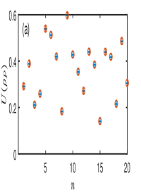
Figure 1: (color online) The measurement-induced non-localities vs $n$. We, respectively, calculated 20 $(3\otimes 3)$-dimensional pure states (a) and 20 $(2\otimes 4)$-dime1nsional qubit-qudit mixed states (b) randomly generated by Matlab R2014b. The ”O” stands for the strictly analytical expressions given by Eq. (22) for (a) and Eq. 26 for (b) and the ”+” marks the numerical expressions given by Eq. (17) in both figures. Both show the perfect consistency.

(iii) The $(3\otimes 3)$-dimensional PPT states.- The $(3\otimes 3)$-dimensional PPT states Alber can be given by

$$\rho_{PPT}=\frac{2}{7}\left|\Phi\right\rangle_{3}\left\langle\Phi\right|+\frac{\alpha}{7}\rho_{+}+\frac{5-\alpha}{7}\rho_{-},\alpha\in[2,4],$$ (27)

where $\left|\Phi\right\rangle_{m}=\frac{1}{\sqrt{m}}\sum_{k=0}^{m-1}\left|kk\right\rangle$, and $\rho_{+}=\frac{1}{3}\sum_{k=0}^{2}\left|k,k\oplus 1\right\rangle\left\langle k,k\oplus 1\right|$and $\rho_{-}=\frac{1}{3}\sum_{k=0}^{2}\left|k\oplus 1,k\right\rangle\left\langle k\oplus 1,k\right|$ with $\oplus$ the modulo-3 addition. The parameter $\alpha$ determines the different quantum correlations of the PPT state. If $\alpha\leq 3$, $\rho_{ppt}$ is separable. When $\alpha\in[3,4]$, the PPT state is entangled. But if $4\leq\alpha\leq 5$, $\rho_{PPT}$ is not a PPT state, but a free entangled state. Based on our definition 1, one can find that $U(\rho_{AB})$ can be analytically calculated for $\alpha\in[2,5]$ as

$$U(\rho_{PPT})=\left\{\begin{array}[]{cc}\frac{21-\sqrt{6(5-\alpha)}-\sqrt{6\alpha}-3\sqrt{\alpha(5-\alpha)}}{31.5},&N_{T}<\alpha\leq 5\\ \frac{4}{21},&2\leq\alpha\leq N_{T}\end{array}\right.,$$ (28)

with $N_{T}=\frac{5+\sqrt{25-4\times(383-34\sqrt{94})/9}}{2}\approx 3.0669$. Both the numerical result based on our theorem and the strictly analytic expression in Eq. (28) are plotted in FIG. 2(a) which shows the perfect consistency between them. In addition, we can analytically find the sudden change point of the measurement-induced non-locality within the entanglement region. As a comparison, we also plot the local quantum uncertainty (LQU) $Q(\rho_{PPT})$ given in Ref. diagon and the measurement-induced non-locality $U(\rho_{PPT})$ in FIG. 2(b). One can find that $U(\rho_{PPT}=Q(\rho_{PPT})$ at their common sudden change point and $U(\rho_{PPT}>Q(\rho_{PPT})$ as expected for other values of $\alpha$.

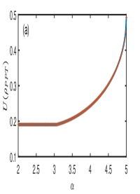
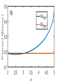
Figure 2: (color online) The measurement-induced non-locality $U(\rho_{PPT})$ for PPT states vs $\alpha$ in (a). The solid line and the ”+” line correspond to the strictly analytical expression of Eq. (28) and the numerical expression of Eq. (17). The sudden change point of the measurement-induced non-locality is about $\alpha\approx 3.0669$. The measurement-induced non-locality is invariant for $\alpha\leq 3.0669$, but becomes increasing for $\alpha>3.0669$. (b) shows the comparison of the LQU $Q(\rho_{PPT})$ and the measurement-induced non-locality $U(\rho_{PPT})$ based on PPT states. The solid line stands for $U(\rho_{PPT})$, while the ”-.” line corresponds to $Q(\rho_{PPT})$. These two lines share a common point at $\alpha\approx 3.0669$. Except this point, $U(\rho_{PPT})$ is always larger than $Q(\rho_{PPT})$ as we expect.

(iv) The $(m\otimes m)$-dimensional isotropic states.- The isotropic states can be given by Alber

$$\rho_{I}=\frac{1-x}{m^{2}-1}\mathbb{I}_{m^{2}}+\frac{m^{2}x-1}{m^{2}-1}\left|\Phi\right\rangle\left\langle\Phi\right|,x\in[-1,1],$$ (29)

with $\left|\Phi\right\rangle_{m}=\frac{1}{\sqrt{m}}\sum_{k=0}^{m-1}\left|kk\right\rangle$. Based on our definition, we can analytically obtain

$$U(\rho_{I})=\frac{m^{2}x-2x+1-2\sqrt{x(1-x)(m^{2}-1)}}{m(1+m)}.$$ (30)

It is obvious that $U(\rho_{I})=0$ for $x=\frac{1}{m^{2}}$. As a comparison, we plot $U(\rho_{I})$ given by Eq. (17) and Eq. (30) in FIG. 3(a). The validity of our theorem is shown again.

(v) The $(m\otimes m)$-dimensional Werner states.- The Werner states can be written as Alber

$$\rho_{W}=\frac{m-x}{m^{3}-m}\mathbb{I}_{m^{2}}+\frac{mx-1}{m^{3}-m}V,x\in[-1,1],$$ (31)

with $V=\sum_{kl}\left|kl\right\rangle\left\langle lk\right|$ the swap operator. The measurement-induced non-locality $U(\rho_{W})$ in terms of our definition can given by

$$U(\rho_{W})=\frac{m-x-\sqrt{(m^{2}-1)(1-x^{2})}}{2(1+m)}.$$ (32)

From Eq. (32), it is shown that $U(\rho_{W})=0$ for $x=\frac{1}{m}$. The comparison between the numerical and the analytic expressions are given in FIG. 3(b) which again shows the perfect consistency.

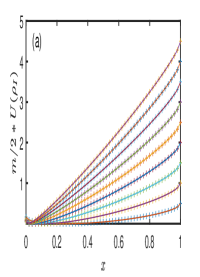
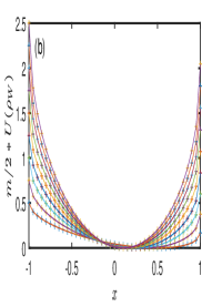
Figure 3: (color online) The measurement-induced non-locality $U(\rho_{I})$ for the Isotropic states (a) and the Werner states (b) vs $x$. The solid line corresponds to the strictly analytical expression of Eq. (30) for (a) and Eq. (32) for (b), while the numerical expressions of Eq. (17) in both figures are marked by the ”+” .

Before the next example, we would like to emphasize that in both example (iv) and example (v), the reduced density matrices $\rho_{A}$ is the maximally mixed state which implies the complete degeneracy. Intuitively, this belongs to the worst case mentioned in the last section (it requires the optimization in the total space of subsystem A). However, in the analytic procedure, one can find that all that are needed to be optimized can be automatically eliminated, which means no optimization is practically required. But it doesn’t mean that the optimization isn’t performed in the numerical procedure. One can find that our numerical method stably approaches the unique optimal solution given in the analytic procedure. In this sense, the two examples provide more powerful proofs for the effectiveness of our theorem than other examples. In addition, considering the dual definitions of the measurement-induced non-locality and LQU, one can find that $U=Q$ for both the isotropic states and the Werner states, since no optimization is practically covered, which is consistent with Ref. remed .

(vi) The $(m\otimes m)$-dimensional degenerate and non-degenerate hybrid states.- In order to demonstrate the practicability of our theorem and avoid the uniform degeneracy of the reduced density matrix, we construct a particular state as

$$\rho_{H}=\frac{\rho_{W}+P}{2}+\frac{(1-m+x)}{2(m^{2}-1)}\left(P-\left|11\right\rangle\left\langle 11\right|\right),x\in[-1,1],$$ (33)

with $P=\frac{1}{n}\sum_{k=2}^{n+1}\left|kk\right\rangle\left\langle kk\right|$ and generally $m\geq 3$ and $n\in[2,m-1]$ to be supposed. The reduced density matrix $\rho_{A}$ of this state has three different eigenvalues. Among them, there could be two degenerate subspaces and one non-degenerate subspace. The eigenvalue $\frac{2m^{2}-mx-m-1}{2m(m^{2}-1)}$ is non-degenerate, the eigenvalue $\frac{m^{3}+mx-1}{2m(m^{2}-1)}$ is $n$-fold degenerate and the eigenvalue $\frac{1}{2m}$ is $(m-n-1)$-fold degenerate. However, one can note that if $m=3$, then $n=2$. Thus $(m-n-1)=0$, i.e., this subspace corresponding to the eigenvalue $\frac{1}{2m}$ doesn’t exist, which implies that the state has two different eigenvalues with only one degenerate subspace. When $m=3$, one can find that the measurement-induced non-locality $U(\rho_{H})$ based on our definition is

$$U(\rho_{H})=\frac{9-3x-6\sqrt{2-2x^{2}}+(2-t)f(x)}{48},$$ (34)

where

$$t=\left\{\begin{array}[]{cc}m,&-1<x\leq-\frac{14}{15}\\ 1,&-\frac{14}{15}<x\leq 1\end{array}\right.,$$ (35)

and

$$f(x)=11+3.5x-\sqrt{(7x+22)(x+1)}$$

$$+2\sqrt{2-2x^{2}}-\sqrt{(4x+44)(1-x)}.$$ (36)

When $m>3$, the measurement-induced non-locality $U(\rho_{H})$ can be given by

$$U(\rho_{H})=\frac{3}{4}-\frac{1}{4(m^{3}-m)}[2(m^{2}-x-1)$$

$$+X_{+}(m-2n)+2Y+(m^{2}-m-2n+2)\sqrt{X_{+}X_{-}}$$

$$+(2n-2)\sqrt{X_{+}+Y}(\sqrt{X_{+}}+\sqrt{X_{-}})],$$ (37)

where $X_{\pm}=(m\mp 1)(1\pm x)$ and $Y=(m^{2}+x-m)\frac{m}{n}$.

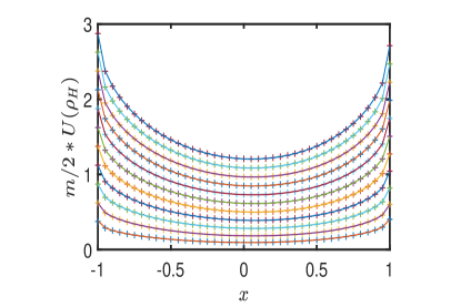
Figure 4: (color online) The measurement-induced non-locality $U(\rho_{H})$ for hybrid states vs $x$. The solid line and the ”+” line correspond to the strictly analytical expression of Eq. (34), Eq. (37) and the numerical expression of Eq. (17).

The comparison of the numerical and the analytic expressions is given in FIG. 4 which again shows the perfect consistency.

(vii) The general quantum states. In order to show the power of our theorem for high-dimensional states, we consider such a state $\rho_{G}$ by mixing a maximally mixed state and a randomly generated $(400\times 400)$-dimensional mixed state $G$ as

$$\rho_{G}=\frac{(1-x)}{400}\mathbb{I}_{400}+xG,x\in[0,1].$$ (38)

Sine the matrix $G$ is too large, it is impossible to explicitly give here. The measurement-induced non-locality versus $x$ has been plotted in FIG. 5. We have uniformly take $51$ points in $x\in[0,1]$ and it averagely takes about $8.4$ seconds for the program (Matlab R2014b) running on the personal laptop (2.8 GHz Intel Core i7/16 GB 1600 MHz DDR3).

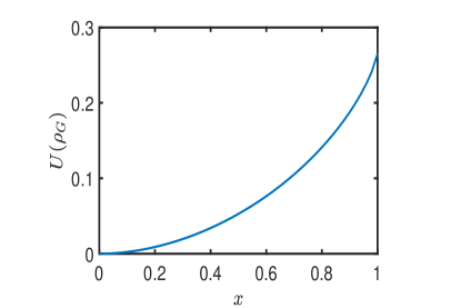
Figure 5: (color online) The measurement-induced non-locality $U(\rho_{G})$ for general hybrid states vs $x$. The solid line corresponds to the numerical expression of Eq. (17).

V Conclusions and discussion

We have redefined the measurement-induced non-locality based on the skew information associated with the broken observable instead of the original high-rank observable. The new definition can solve the non-contractivity problem in the previous measurement-induced non-locality based on the $l_{2}$ norm and has obvious operational meaning in terms of quantum metrology. It allows us to analytically calculate the measurement-induced non-locality of the pure states, the qubit-qudit states, and some large classes of high-dimensional states. In particular, the new definition enables us to develop the powerful inverse approximate joint diagonalization algorithm based on the very remarkable Jacobi method for the approximate joint diagonalization problem. It is shown that this inverse approximate joint diagonalization algorithm similar to the corresponding approximate joint diagonalization algorithm has good effectiveness such as simplicity, stability, high efficiency and state independence. This is further proven by the detailed comparisons between the analytic and the numerical results of various examples. Compared with the diagonalization of a single density matrix, it is shown that our measurement-induced non-locality has even the almost analytic expression for any quantum state, which gives an alternative effective means for the computability of the measurement-induced non-locality.

Finally, we would like to emphasize that the method to breaking observable isn’t a trivial skill but has many successful applications and can conquer many key problems in quantum discord and especially in quantum coherence. The potential application is worth our forthcoming attention. In addition, considering the quantum resource theory, it could be usually impossible for a general state to find an analytic quantifier of a general quantum resource, so how to develop an effective numerical means should be a quite necessary problem. The power exhibited by the inverse approximate joint diagonalization and the approximate joint diagonalization algorithms could shed new light on both the resource theory and the other aspects of physics.

- (1) C.H. Bennett, H.J. Bernstein, S. Popescu, and B. Schumacher, Concentrating partial entanglement by local operations, Phys. Rev. A 53, 2046 (1996).
- (2) C. H. Bennett, D. P. DiVincenzo, J. A. Smolin, and W. K. Wootters, Mixed-state entanglement and quantum error correction, Phys. Rev. A 54, 3824 (1996).
- (3) C. H. Bennett, G. Brassard, S. Popescu, B. Schumacher, J. A. Smolin, and W. K. Wootters, Purification of Noisy Entanglement and Faithful Teleportation via Noisy Channels, Phys. Rev. Lett. 76, 722 (1996).
- (4) P. Horodecki, R. Horodecki, Distillation and bound entanglement, Quant. Inf. Comp. 1, 45 (2000).
- (5) W. K. Wootters, Entanglement of formation and concurrence, Quant. Inf. Comp. 81, 865 (2009).
- (6) R. Horodecki, P. Horodecki, M. Horodecki and K. Horodecki, Quantum entanglement, Rev. Mod. Phys. 81, 865 (2009).
- (7) L. Henderson, V. Vedral, Classical, quantum and total correlations, J. Phys. A, Math. Theor. 34 6899 (2001).
- (8) H. Ollivier, W. H. Zurek, Quantum discord: A measure of the quantumness of correlations, Phys. Rev. Lett. 88 017901 (2001).
- (9) A. Datta, A. Shaji, and C. M. Caves, Quantum discord and the power of one qubit, Phys. Rev. Lett. 100, 050502 (2008).
- (10) T. Tufarelli, D. Girolami, R. Vasile, S. Bose, and G. Adesso, Quantum resources for hybrid communication via qubit-oscillator states, Phys. Rev. A 86, 052326 (2012).
- (11) C. S. Yu, J. Zhang, and H. Fan, Quantum dissonance is rejected in an overlap measurement scheme, Phys. Rev. A 86, 052317 (2012).
- (12) A. Brodutch, Discord and quantum computational resources, Phys. Rev. A 88, 022307 (2013).
- (13) T. Baumgratz, M. Cramer, and M. B. Plenio, Quantifying coherence, Phys. Rev. Lett. 113, 140401 (2014).
- (14) A. Winter and D. Yang, Operational resource theory of coherence, Phys. Rev. Lett. 116, 120404 (2016).
- (15) E. Chitambar and M. H. Hsieh, Relating the resource theories of entanglement and quantum coherence, Phys. Rev. Lett. 117, 020402 (2016).
- (16) A. Streltsov, S. Rana, P. Boes and J. Eisert, Structure of the resource theory of quantum coherence, Phys. Rev. Lett. 119, 140402 (2017).
- (17) K. B. Dana, M. G. Díaz, M. Mejatty and A. Winter, Resource theory of coherence: beyond states, Phys. Rev. A 95, 062327 (2017).
- (18) A. Streltsov, S. Rana, M. N. Bera and M. Lewenstein, Towards resource theory of coherence in distributed scenarios, Phys. Rev. X 7, 011024 (2017).
- (19) F. G. S. L. Brandão, M. Horodecki, J. Oppenheim, J. M. Renes, and R. W. Spekkens, Resource theory of quantum states out of thermal equilibrium, Phys. Rev. Lett. 111, 250404 (2013).
- (20) F. G. S. L. Brandão and G. Gour, Reversible framework for quantum resource theories, Phys. Rev. Lett. 115, 070503 (2015).
- (21) C. S. Yu, Quantum coherence via skew information and its polygamy, Phys. Rev. A 95, 042337 (2017).
- (22) A. Peres, Separability criterion for density matrices, Phys. Rev. Lett. 77, 1413 (1996).
- (23) W. K. Wootters, Entanglement of formation of an arbitrary state of two qubits, Phys. Rev. Lett. 80, 2245 (1998).
- (24) G. Vidal, and R. F. Werner, Computable measure of entanglement, Phys. Rev. A 65, 032314 (2002).
- (25) S. L. Luo, Quantum discord for two-qubit systems, Phys. Rev. A 77, 042303 (2008).
- (26) S. L. Luo, Using measurement-induced disturbance to characterize correlations as classical or quantum, Phys. Rev. A 77, 022301 (2008).
- (27) B. Dakić, V. Vedral, and Č. Brukner, Necessary and sufficient condition for nonzero quantum discord, Phys. Rev. Lett. 105, 190502 (2010).
- (28) D. Girolami, T. Tufarelli, and G. Adesso, Characterizing nonclassical correlations via local quantum uncertainty, Phys. Rev. Lett. 110, 240402 (2013).
- (29) C. S. Yu, S. X. Wu, X. G. Wang, X. X. Yi and H. S. Song, Quantum correlation measure in arbitrary bipartite systems, Europhys. Lett. 107, 10007 (2017).
- (30) F. Mintert, M. Kuś, and A. Buchleitner, Concurrence of mixed bipartite quantum states in arbitrary dimensions, Phys. Rev. Lett. 92, 167902 (2004).
- (31) K. Chen, S. Albeverio and S. M. Fei, Concurrence of arbitrary dimensional bipartite quantum states, Phys. Rev. Lett. 95, 040504 (2005).
- (32) C. S. Yu, and H. S. Song, Separability criterion of tripartite qubit systems, Phys. Rev. A 72, 022333 (2005).
- (33) K. Audenaert, F. Verstraete, and B. D. Moor, Variational characterizations of separability and entanglement of formation, Phys. Rev. A 64, 052304 (2001).
- (34) M. A. Jafarizadenh, M. Mirzaee, and M. Rezaee, Best separable approximation with semi-definite programming method, Int. J. Quant. Inf. 2, 541 (2004).
- (35) J. Řeháček and Z. Hradil, Quantification of entanglement by means of convergent iterations, Phys. Rev. Lett. 90, 127904 (2003).
- (36) Y. Zinchenko, S. Friedland, and G. Gour, Numerical estimation of the relative entropy of entanglement, Phys. Rev. A 82, 052336 (2010).
- (37) K. Cao, Z. W. Zhou, G. C. Guo and L. X. He, Efficient numerical method to calculate the three-tangle of mixed states, Phys. Rev. A 81, 034302 (2010).
- (38) B. Röthlisberger, J. Lehmann and D. Loss, Comp. Phys. Commu. 183, 155 (2012).
- (39) B. Röthlisberger, J. Lehmann, D. S. Saraga, P. Traber and D. Loss, Highly entangled ground states in tripartite qubit systems, Phys. Rev. Lett. 100, 100502 (2008).
- (40) B. Röthlisberger, J. Lehmann and D. Loss, Numerical evaluation of convex-roof entanglement measures with applications to spin rings, Phys. Rev. A 80, 042301 (2009).
- (41) C. Napoli, T. R. Bromley, M. Cianciaruso, M. Piani, N. Johnston and G. Adesso, Robustness of coherence: an operational and observable measure of quantum coherence, Phys. Rev. Lett. 116, 150502 (2016).
- (42) M. Piani, M. Cianciaruso, T. R. Bromley, C. Napoli, N. Johnston and G. Adesso, Robustness of asymmetry and coherence of quantum states, Phys. Rev. A 93, 042107 (2016).
- (43) S. Rana, P. Parashar and M. Lewenstein, Trace-distance measure of coherence, Phys. Rev. A 93, 012110 (2016).
- (44) P. Zanardi, G. Styliaris and L. C. Venuti, Measures of coherence-generating power for quantum unital operations, Phys. Rev. Lett. 95, 052307 (2017).
- (45) S. L. Luo and S. S. Fu, Measurement-Induced Nonlocality, Phys. Rev. Lett. 106, 120401 (2011).
- (46) S. L. Luo, and S. S. Fu, Geometric measure of quantum discord, Phys. Rev. A 82, 034302 (2010).
- (47) M. Piani, Problem with geometric discord, Phys. Rev. A 86, 034101 (2012).
- (48) S. Y. Mirafzali, I. Sargolzahi, A . Ahanj, K. Javidan, and M. Sarbishaei, Measurement-induced nonlocality for an arbitrary bipartite state, Quant. Inf. Comp. 13, 0479 (2011).
- (49) A. Sen, D. Sarkar, and A. Bhar, Monogamy of measurement-induced nonlocality, J. Phys. A Math. Theor., 45, 405306 (2012).
- (50) S. Rana, and P. Parashar, Geometric discord and measurement-induced nonlocality for well known bound entangled states, Quant. Inf. Proc. 12, 2523 (2013).
- (51) S. X. Wu, J. Zhang, C. S. Yu, and H. S. Song, Uncertainty-induced quantum nonlocality, Phys. Letts. A 378, 344 (2014).
- (52) M. L. Hu, and H. Fan, Measurement-induced nonlocality based on the trace norm, New. J. Phys. 17,033004 (2015).
- (53) L. D. Wang, L. T. Wang, M. Yang, J. Z. Xu, Z. D. Wang, and Y. K. Bai, Entanglement and measurement-induced nonlocality of mixed maximally entangled states in multipartite dynamics, Phys. Rev. A 93, 062309 (2016).
- (54) Z. J. Xi, X. G. Wang and Y. M. Li, Measurement-induced nonlocality based on the relative entropy, Phys. Rev. A 85, 042325 (2012).
- (55) E. P. Wiger and M. M. Yanase, Information contents of distributions, Proc. Natl. Acad. Sci. USA, 49, 910 (1963).
- (56) E. H. Lieb, Convex trace functions and the Wigner-Yanase-Dyson conjecture, Adv. Math. 11, 267 (1973).
- (57) S. L. Luo, Wigner-Yanase skew information and uncertainty relations, Phys. Rev. Lett. 91, 180403 (2003).
- (58) U. Dorner, R. Demkowicz-Dobrzanski, B. J. Smith, J. S. Lundeen, W.Wasilewski, K. Banaszek, and I. A. Walmsley, Phys. Rev. Lett. 102, 040403 (2009).
- (59) S. L. Braunstein and C. M. Caves, Phys. Rev. Lett. 72, 3439 (1994);
- (60) S. L. Braunstein, C. M. Caves, and G. J. Milburn, Ann. Phys. (N.Y.)247, 135 (1996).
- (61) S. L. Luo, Proc. Am. Math. Soc. 132, 885 (2003).
- (62) J. F. Cordoso, and A. Souloumiac, Blind beamforming for non-Gaussian signals, Radar & Signal Processing, IEE Proceedings-F 140, 362 (1993).
- (63) J. F. Cordoso, and A. Souloumiac, Jacobo angles for simultaneous diagonalization, SIAM J. Mater. Anal. Appl. 17, 161 (1996).
- (64) A. Ziehe, P. Laskov, G. Nolte, and K.R. Müller, A fast algorithm for joint diagonalization with non-orthogonal transformations and its application to blind source separation, J. Mach. Learn. Res. 5, 777 (2004).
- (65) G. H. Golub, and C. F. Van Loan, Matrix Computations, 3rd edition (The Johns Hopkins University Press, 1996).
- (66) C. F. Van Loan, and N. P. Pitsianis, Linear algebra for large scale and real time applications, edited by M. S. Moonen and G. H. Golub, (Kluwer, Dordrecht, pp. 293–314, 1993).
- (67) G. Alber, T. Beth, M. Horodecki, P. Horodecki, R. Horodecki, M. Rötteler, H. Weinfurter, R. Werner, and A. Zeilinger, Quantum Information: An Introduction to Basic Theoretical Concepts and Experiments, (Springer-Verlag, Berlin, Heidelberg, 2001).
- (68) L. N. Chang, and S. L. Luo, Remedying the local ancilla problem with geometric discord, Phys. Rev. A 87, 062303 (2013).