Spectral signatures of non-thermal baths in quantum thermalization

Abstract

We show that certain coherences, termed as heat-exchange coherences, which contribute to the thermalization process of a quantum probe in a repeated interactions scheme, can modify the spectral response of the probe system. We suggest to use the power spectrum as a way to experimentally assess the apparent temperature of non-thermal atomic clusters carrying such coherences and also prove that it is useful to measure the corresponding thermalization time of the probe, assuming some information is provided on the nature of the bath. We explore this idea in two examples in which the probe is assumed to be a single-qubit and a single-cavity field mode. Moreover, for the single-qubit case, we show how it is possible to perform a quantum simulation of resonance fluorescence using such repeated interactions scheme with clusters carrying different class of coherences.

I Introduction

In the rapidly growing field of quantum thermodynamics Vinjanampathy and Anders (2016); Goold et al. (2016); Alicki and Kosloff (2018); Deffner and Campbell (2019) several new effects that could bend the rules Merali (2017) of the classical theory are being predicted. Especially, developments related with the performance of non-thermal quantum machines constitute a good example to these effects, with which one can extend the limits dictated by the classical thermodynamics by exploiting the quantumness of the bath that the system of interest is interacting Scully (2002); Scully et al. (2003); Dağ et al. (2019); Manatuly et al. (2019); Hardal and Müstecaplıoğlu (2015); Türkpençe and Müstecaplıoğlu (2016); Quan et al. (2006); Liao et al. (2010); Dağ et al. (2016); Çakmak et al. (2017); Roßnagel et al. (2014); Niedenzu et al. (2016, 2018). The distinguishing property of such non-thermal baths is that they possess some amount of quantum coherence, and as a result they can not be described by a thermal state. A natural question at this point would be to ask about the effects of the coherences in the bath on the dynamics of the central system while they are in contact. It has been shown that it is possible to fully characterize the types of coherences in a non-thermal bath. While some coherences have a displacing or squeezing effects, there are certain types of coherences that merely contribute to the thermalization of the system, which are dubbed as heat-exchange coherences (HECs) Dağ et al. (2016); Çakmak et al. (2017); Dağ et al. (2019); Manatuly et al. (2019). Therefore, non-thermal baths that only contain HECs act as an effective heat bath for the probe at a certain apparent temperature. The apparent temperature was recently introduced in Latune et al. (2019) and it is based on the expression of the heat flow between, in general, out-of-equilibrium quantum systems. If one of the systems can be described as a bath, the apparent temperature coincides with notion of local temperature for stationary non-equilibrium baths Alicki and Gelbwaser-Klimovsky (2015); Alicki (2014).

How to assign an apparent temperature to these non-thermal baths and how to test their corresponding quantum thermodynamic predictions from the spectroscopic point of view are the questions that lie at the heart of this contribution. We present a method that relies on the power spectrum of the probe system to assess the apparent temperature of the bath for which it is possible to show that, with some previous information of the bath, one can separately identify the effects of a thermal and a non-thermal, coherent bath. Moreover, the information about the thermalization time of the probe can also be extracted from the power spectrum. The presented method is actually along the same lines with the recent efforts in quantum thermometry, which tries to estimate the temperature of an environment by quantum probes Pasquale and Stace (2018); Stace (2010); Pasquale et al. (2016); De Palma et al. (2017); De Pasquale et al. (2017); Mehboudi et al. (2019); Razavian et al. (2019); Campbell et al. (2017, 2018); Correa et al. (2015); Hofer et al. (2017). Specifically, the present approach resembles the one adopted in Razavian et al. (2019), in which the authors take advantage of the dephasing dynamics of a qubit that is embedded in an environment to assign a temperature to that environment. However, in this work, the environment with which the probe is interacting need not to be a thermal one and can contain certain coherences that appears as an apparent temperature to the probe.

In particular, we generalize the previous settings presented in Dağ et al. (2016); Çakmak et al. (2017); Dağ et al. (2019); Manatuly et al. (2019) and consider a probe system that is both in contact with a thermal and a non-thermal bath that only contain HECs, and address the aforementioned matter of thermalization dynamics by considering two simple, but not trivial, examples in the weak coupling regime. We begin by considering a central single-qubit as our probe [see Fig. 1(a)] which is interacting with a $N$-qubit coherent cluster (non-thermal bath) together with a thermal bath and derive some of their quantum thermodynamic effects on the probe, including the thermalization temperature and time. Then, we replace the qubit by a single electromagnetic field mode as our probe [see Fig. 1(b)], and we show that the apparent field temperature is the same as the qubit case, however, their respective thermalization times are completely different. Interestingly, when coherences that are different from HECs are considered to be present in the $N$-qubit cluster, this scheme can also be used to perform a quantum simulation of resonance fluorescence in an ordinary or squeezed vacuum in free space.

The rest of the manuscript is organized as follows. In Sec. II, we introduce our model to manipulate the temperature of a quantum probe by interacting it with an $N$-qubit cluster that possess certain coherences. Sec. III presents our results on how to assess the apparent temperature of the coherent qubit clusters, and thermalization time of the quantum probe by looking at the stationary power spectrum of it. Also, we provide fundamental bounds on how well we can estimate the apparent temperature and the HECs of the non-thermal bath. In Sec. IV, by adopting a time-dependent physical spectrum, we identify which types of coherences can be used to shape the spectral response of the qubit probe and make a quantum simulation of resonance fluorescence. Sec. V includes our discussion on the possible experimental applications of the proposed scheme and we conclude in Sec. VI.

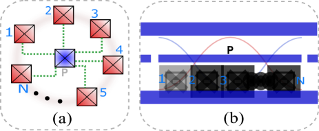
Figure 1: (Color online) Schematic representations of a repeated interaction schemes also known as generalized micromaser setups. (a) A central probe qubit (blue central box) interacts simultaneously with $N$-qubits (red surrounding boxes) acting as a non-thermal bath. (b) A single-electromagnetic field mode (blue thin rectangle) interacting collectively with a similar $N$-qubit cluster. These setups resemble the ones used in the field of circuit-QED, where boxes represent superconducting qubits and long rectangles are 1D transmission line resonators. However, setups based on cavity-QED architecture where an atomic cluster beam traverse a 3D electromagnetic cavity will also work.                                      

II Models of quantum-thermalizing machines

Throughout this section we present some properties of the thermalization dynamics associated with two different types of quantum probes embedded in non-thermal baths and subject to diverse dissipative and decohering processes. In the spirit of the references Liao et al. (2010); Scarani et al. (2002), we call our scheme as quantum-thermalizing machines, in which a central system relax to a thermal equilibrium state upon repeatedly interacting with a series of reservoir particles. Similar results have also obtained by the authors in Ref. Manatuly et al. (2019) in the absence of a thermal photon bath and decoherence. These properties shall be the basis and motivation for further study of the power spectrum associated with the probe in Sec. III and the respective characterization of them by means of spectroscopic measurements.

II.1 Single qubit probe for an non-thermal bath of $N$-qubit clusters

First, let us consider our central system as a single-qubit, with self-Hamiltonian $H_{q}\!=\!\hbar\omega_{q}\sigma_{z}/2$ of frequency $\omega_{q}$, embedded in a thermal photon bath and also interacting collectively during a time “$\tau$” at a rate $p$ with an environment made of $N$ identical qubits [see Fig. 1(a)] that we will call it the cluster $H_{\rm cl}\!=\!\sum_{j}\hbar\omega_{q}\sigma_{z}^{j}/2$, through a dipolar interaction $H_{\rm dip}$​=​$\sum_{j}\hbar g(\sigma_{+}^{j}\sigma_{-}$+$\sigma_{-}^{j}\sigma_{+})$. Here, $g$ is the interaction strength, $\sigma_{z}^{j}$ and $\sigma_{\pm}^{j}$ are the usual Pauli $z$ and ladder operators of the $j=1,2,..N$-th qubit, respectively with $[\sigma_{z}^{i},\sigma_{\pm}^{j}]\!=\!\pm 2\sigma_{\pm}^{i}\delta_{ij}$ and $[\sigma_{+}^{i},\sigma_{-}^{j}]\!=\!\sigma_{z}^{i}\delta_{ij}$. Without ambiguity, operators without superscript $j$ will refer to the central qubit system. Following the approach adopted for the micromaser theory Filipowicz et al. (1986), we will assume that before each interaction the state of the $N$-qubit cluster has to be reset to its initial state $\rho_{\rm cl}$. Under this assumption, it is possible to derive a Markovian master equation for the single-qubit density matrix $\rho_{q}$. Thereby, tracing out the degrees of freedom of the cluster and the thermal bath, in the interaction picture associated with the self Hamiltonian of the central qubit, and up to second order in $g\tau$ we get (see Appendix A for a detailed derivation):

$$\dot{\rho}_{q}=r_{d}\mathcal{L}[\sigma_{-}]\rho_{q}+r_{e}\mathcal{L}[\sigma_{+}]\rho_{q}+{\gamma_{\phi}}\mathcal{L}[\sigma_{z}/4]\rho_{q},$$ (1)

where $\mathcal{L}[o]\rho_{q}\equiv 2o\rho_{q}o^{\dagger}-o^{\dagger}o\rho_{q}-\rho_{q}o^{\dagger}o$ is the usual Lindblad super-operator. $r_{e}=[\mu_{q}\langle J_{+}J_{-}\rangle+\gamma\bar{n}_{\rm en}]/2$ and $r_{d}=[\mu_{q}\langle J_{-}J_{+}\rangle+\gamma(\bar{n}_{\rm en}+1)]/2$ are the excitation (heating) and de-excitation (cooling) rates, respectively, with $\mu_{q}=p(g\tau)^{2}$ is the effective coupling rate and $\bar{n}_{\rm en}=(\exp[\hbar\omega_{q}/(k_{B}T_{\rm en})]-1)^{-1}$ is the average photon number of a possibly unavoidable background thermal environment at temperature $T_{\rm en}$ that it is in contact with the central qubit system. $J_{\pm}=\sum_{j}\sigma_{\pm}^{j}$ and $J_{z}=\sum_{j}\sigma_{z}^{j}/2$ are the collective spin operators Ban (1993). It is known that dissipation of energy and dephasing have a dramatic impact on the performance of quantum thermal and non-thermal machines. For instance, making use of dissipation in the photon field and pure atomic dephasing the quantum-classical transition of a photon-Carnot engine was evidenced in Quan et al. (2006). Here, those decoherence processes are incorporate, phenomenologically in Eq. (1), through the qubit spontaneous emission (SE) coefficient $\gamma$ and a nonradiative dephasing rate $\gamma_{\phi}$.

Coherences of $\rho_{\text{cl}}$ that contribute to the average value $\langle J_{-}J_{+}\rangle={\rm Tr}\{\rho_{\rm cl}J_{-}J_{+}\}$ and its complex conjugate were identified as the HECs of the $N$-qubit cluster Manatuly et al. (2019); Çakmak et al. (2017); Dağ et al. (2016) which, in turn, act as an environment with an apparent temperature to the central qubit system. Therefore, along this work, we will be interested in determining $\langle J_{\pm}J_{\mp}\rangle$ and their influence on the quantum evolution of the central system.

Equation (1) has the following solution for its density matrix elements Breuer et al. (2002):

$$\rho_{eg}(t) =\rho_{eg}(0)\exp\left[-\left(r_{d}+r_{e}+\gamma_{\phi}\right)t\right],$$ (2a)

$$\rho_{ee}(t) =\frac{[r_{d}\rho_{ee}(0)-r_{e}\rho_{gg}(0)]e^{-2t\left(r_{d}+r_{e}\right)}+r_{e}}{r_{d}+r_{e}},$$ (2b)

$\rho_{ge}(t)=\rho_{eg}(t)^{*}$ and $\rho_{gg}(t)=1-\rho_{ee}(t)$. We have used the notation $\rho_{eg}=\langle e|\rho_{q}|g\rangle$, $\rho_{ee}=\langle e|\rho_{q}|e\rangle$, $\rho_{gg}=\langle g|\rho_{q}|g\rangle$ and $\rho_{ge}=\langle g|\rho_{q}|e\rangle$, where $|g\rangle$ ($|e\rangle$) is the ground (excited) qubit state.

Defining the internal energy of the system as $E_{q}={\rm Tr}\{\rho_{q}H_{q}\}$, the heat flow from a non-thermal bath to the qubit probe is given by $\dot{Q}_{q}=\dot{E}_{q}={\rm Tr}\{\dot{\rho}_{q}H_{q}\}$. Using Eq. (1) it is easy to show that $\dot{Q}_{q}=2\hbar\omega_{q}\big{[}r_{e}\rho_{gg}(t)-r_{d}\rho_{ee}(t)\big{]}$, which can be rewritten in the following form

$$\dot{Q}_{q}=2\hbar\omega_{q}r_{d}\rho_{gg}\big{[}\exp(-\hbar\omega_{q}/k_{B}T_{B})-\exp(-\hbar\omega_{q}/k_{B}T_{q})\big{]},$$ (3)

where $k_{B}$ is the Boltzmann constant, $T_{q}$ and $T_{B}$ are the apparent temperatures of the qubit probe and the non-thermal bath respectively. These are defined as Latune et al. (2019)

$$T_{q}=\frac{\hbar\omega_{q}}{k_{B}}\Big{[}\ln\left(\frac{\rho_{gg}(t)}{\rho_{ee}(t)}\right)\Big{]}^{-1},\quad T_{B}=\frac{\hbar\omega_{q}}{k_{B}}\Big{[}\ln\Big{(}\frac{r_{d}}{r_{e}}\Big{)}\Big{]}^{-1}.$$ (4)

One can also see that $T_{q}$ and $T_{B}$ can be viewed as temperatures due to the fact that they determine the sign of the heat current, i.e. $\dot{Q}_{q}$ is positive if $T_{q}\geq T_{B}$. Notice that $T_{q}$ ($T_{B}$) is, in principle, a time-dependent (time-independent) parameter that depends on the state of the probe (bath), which can be thermal or non-thermal. In fact, if we switch-off the repeated interaction with the $N$-qubit cluster, $\mu_{q}=0$, the apparent temperature $T_{B}$ is equal to the temperature of the background thermal environment $T_{\rm en}$. In the steady state $\rho_{q}^{st}$ is a statistical mixture of its excited and ground states with probabilities $\rho_{ee}^{st}=\rho_{ee}(\infty)=r_{e}/(r_{d}+r_{e})$ and $\rho_{gg}^{st}=\rho_{gg}(\infty)=r_{d}/(r_{d}+r_{e})$ respectively. Moreover, $\rho_{gg}^{st}/\rho_{ee}^{st}=r_{d}/r_{e}$, therefore, at the steady state the qubit probe thermalise at the apparent temperature of the non-thermal bath. Hence, the qubit temperature can be controlled by the ratio between the cooling and heating rates. $T_{q}$ can also be obtained only by looking for the population of the qubit excited steady state since $T_{q}=(\hbar\omega_{q}/k_{B})[\ln(\rho_{ee}^{st-1}-1)]^{-1}$. Note that the apparent temperature of the qubit probe can have negative values at the steady state, i.e. it is possible to invert the populations of the probe, if $r_{e}>r_{d}$. This condition translates into the expectation values in the following way $\langle J_{+}J_{-}\rangle-\langle J_{-}J_{+}\rangle>\gamma/\mu_{q}$ and is only satisfiable if we have an inverted population in the bath states. Eventhough HECs have no role in determining this condition since they contribute to both expectation values with the same amount, they can be used as a knob to enhance the negative apparent temperature through their dependence on the apparent temperature $r_{d}/r_{e}$, as presented in Eq. (4). Significance of this result is that even a set of weakly inverted qubits, slightly above the effective infinite temperature, can be used as a fully inverted system, with the aid of sufficient quantum coherence.

From Eqs. (2a) and (2b), we see that $\gamma_{\phi}$ only affects the off-diagonal density matrix elements, which implies that dephasing does not change either $T_{q}$ or the qubit thermalization time $t_{q}\equiv[2(r_{d}+r_{e})]^{-1}$. The latter can be rewritten as

$$t_{q}=\frac{1}{\gamma(2\bar{n}_{\rm en}+1)+2\mu_{q}(\langle J^{2}\rangle-\langle J_{z}^{2}\rangle)},$$ (5)

where $J^{2}=J_{z}^{2}+(J_{+}J_{-}+J_{-}J_{+})/2$ is the Casimir operator of $\mathfrak{su}(2)$ Ban (1993).

II.2 Single cavity probe for an non-thermal bath of $N$-qubit clusters

Now we replace the single-qubit central system from the previous example by a single electromagnetic field mode $H_{c}=\hbar\omega_{c}a^{\dagger}a$ of frequency $\omega_{c}$ inside a leaky cavity. The resonant collective interaction (of strength $\lambda$) between the field and the $N$-qubit coherent clusters, is governed by the Tavis-Cummings (TC) Hamiltonian $H_{\text{TC}}=\lambda(J_{+}a+J_{-}a^{\dagger})$ Tavis and Cummings (1968). Here, $a$ ($a^{\dagger}$) is the usual annihilation (creation) bosonic field operator that satisfy $[a,a^{\dagger}]=1$. This kind of collective interaction has been realized experimentally with $N=3$ Fink et al. (2009) (and $N=6$ Yang et al. (2018)) fully controllable superconducting qubits embedded in a transmission line resonator, where the coupling strengths between the qubits and the resonator were virtually identical. A schematic representation of the TC model is sketched in Fig. 1(b). Under the standard assumptions of the micromaser theory Filipowicz et al. (1986); Scully and Zubairy (1997); Temnov (2005) and within the aforementioned conditions, the following Markovian master equation for the electromagnetic field density matrix $\rho_{c}$ (in a rotating frame at the cavity frequency) can be derived Dağ et al. (2016); Strasberg et al. (2017) (see Appendix A):

$$\dot{\rho}_{c}=\mathcal{R}_{d}\mathcal{L}[a]\rho_{c}+\mathcal{R}_{e}\mathcal{L}[a^{\dagger}]\rho_{c}+\kappa_{\phi}\mathcal{L}[a^{\dagger}a]\rho_{c},$$ (6)

Once again, $\mathcal{R}_{d}$=$[\mu_{c}\langle J_{-}J_{+}\rangle+\kappa(\bar{n}_{\rm en}+1)]/2$ and $\mathcal{R}_{e}$=$[\mu_{c}\langle J_{+}J_{-}\rangle+\kappa\bar{n}_{\rm en}]/2$ represent the cooling and heating rates respectively. $\kappa$ ($\kappa_{\phi}$) is the cavity field decay (dephasing) rate and $\bar{n}_{\text{en}}$ now depends on the $\omega_{c}$ instead of $\omega_{q}$. Like in the previous case $\mu_{c}=p(\lambda\tau)^{2}$ is the effective coupling rate. To elucidate how the HECs intervene in the cavity field evolution, we first calculate the corresponding equations of motion for the photon number $a^{\dagger}a$ and field $a$ operators, these are given by $\langle\dot{a^{\dagger}a}\rangle_{t}=-2(\mathcal{R}_{d}-\mathcal{R}_{e})\langle a^{\dagger}a\rangle_{t}+2\mathcal{R}_{e}$ and $\langle\dot{a}\rangle_{t}=-(\mathcal{R}_{d}-\mathcal{R}_{e}+\kappa_{\phi})\langle a\rangle_{t}$. The notation $\langle\mathcal{O}\rangle_{t}={\rm Tr}\{\rho_{c}\mathcal{O}(t)\}$ was used. Taking the initial conditions $\langle a^{\dagger}a\rangle_{0}$ and $\langle a\rangle_{0}$ their solutions are: $\langle a^{\dagger}a\rangle_{t}=n_{st}+(\langle a^{\dagger}a\rangle_{0}-n_{st})\exp[-2(\mathcal{R}_{d}-\mathcal{R}_{e})t]$ and $\langle a\rangle_{t}=\langle a\rangle_{0}\exp[-(\mathcal{R}_{d}-\mathcal{R}_{e}+\kappa_{\phi})t]$, where $n_{st}=\mathcal{R}_{e}(\mathcal{R}_{d}-\mathcal{R}_{e})^{-1}$ is the steady state photon number. Substituting the values of the excitation and de-excitation rates yields $n_{st}$=$({\kappa\bar{n}_{\rm en}+\mu_{c}\langle J_{+}J_{-}\rangle})$/ $({\kappa-2\mu_{c}\langle J_{z}\rangle})$. The heat flow from a non-thermal bath to the field mode is $\dot{Q}_{c}={\rm Tr}\{\dot{\rho}_{c}H_{c}\}$. Using Eq. (6) this reduces to $\dot{Q}_{c}=2\hbar\omega_{c}\big{(}\mathcal{R}_{e}\langle aa^{\dagger}\rangle_{t}-\mathcal{R}_{d}\langle a^{\dagger}a\rangle_{t}\big{)}$. Rewriting this expression in the form of Eq. (3), we can obtain the apparent temperature of the field mode given by $T_{c}=(\hbar\omega_{c}/k_{B})[\ln\big{(}\langle a^{\dagger}a\rangle_{t}^{-1}+1\big{)}]^{-1}$. As expected, at the steady state, the field probe thermalise at the apparent temperature of the non-thermal bath, i.e., $T_{B}=(\hbar\omega_{c}/k_{B})\ln(\mathcal{R}_{d}/\mathcal{R}_{e})^{-1}$. On the other hand, thermalization time of the field mode is given by $t_{c}\equiv[2(\mathcal{R}_{d}-\mathcal{R}_{e})]^{-1}$, which can be rewritten in terms of the total population inversion $\langle J_{z}\rangle$ as:

$$t_{c}=\frac{1}{\kappa-2\mu_{c}\langle J_{z}\rangle}.$$ (7)

The interaction of the central system with the $N$-qubit coherent cluster can modify its natural (or fabricated) parameters. For instance, if $\kappa_{\phi}=0$, the coherence time of field mode is equal to $2t_{c}$, thus, from Eq. (7) it is clear that $2t_{c}$ can be enhanced just by having, for example, a large number of environmental qubits in their excited state, this could improve the performance of a thermal machine using the field mode as the probe. Such a situation is especially useful when changing the quality factor of a cavity (or transmission line resonator) is difficult due to manufacturing limitations.

Lastly, we would like to comment on the possibility of negative temperatures in the present case. Such a situation only occurs when $\mathcal{R}_{d}<\mathcal{R}_{e}$, however this condition implies that the thermalization time $t_{c}$ can be infinite or even negative. Moreover, the steady-state photon number $n_{st}=\mathcal{R}_{e}(\mathcal{R}_{d}-\mathcal{R}_{e})^{-1}$ also beomes ill-defined. These problems have their roots in the fact that it is not possible for a quantum harmonic oscillator to attain negative temperatures, since its energy spectrum is not bounded from above.

II.3 Bath size effects on the probe thermalization

So far, we can point out some important things regarding thermalization of the single-qubit system and the single-field mode. Despite the fact that $T_{q}$ and $T_{c}$ look different, they are defined as the logarithm of the ratio between their respective heating and cooling rates. Consequently, both temperatures have the same dependency on $\langle J_{\pm}J_{\mp}\rangle$. This implies that the only difference between both temperatures should be attributed to the corresponding parameters that characterize each physical system. However, there must be some situations, of practical purposes, in which it would be more advantageous to work with a cavity field mode (resonator) instead of a single-qubit as the main central system or vice versa. As an example, let’s consider the initial state of $N$-qubit cluster to be a Dicke state $\rho_{\text{cl}}=|k,N\rangle\langle k,N|$. This is a non-thermal state prepared by non-thermal means where $k$ is the number of excitations in the cluster and $\langle J_{+}J_{-}\rangle=k(N-k+1)$, $\langle J_{-}J_{+}\rangle=(k+1)(N-k)$ and $\langle J_{\pm}\rangle=\langle J_{\pm}^{2}\rangle=0$ Klimov and Chumakov (2009). If one considers a Dicke state that is close to the central block, i.e. setting $k=N/2-1$, it is possible to see from the above expressions that $T_{q}$ and $T_{c}$ grow with $N^{2}$, see Ref. Manatuly et al. (2019) for a detailed derivation. This superlinear scaling is fundamentally based upon symmetries of Dicke-type states. An easy interpretation could be their relation to possible ways of selecting pairs of states among N degenerate ones, which scales as $N^{2}$. However, the corresponding thermalization times (using the Dicke states and $k=N/2-1$) are quite different; $t_{q}$ is inversely proportional to $N^{2}$ Manatuly et al. (2019) and $t_{c}$ will be independent of the number of environmental qubits. Hence, if there is a difference between the thermalization time of a bosonic and fermionic probes, this should be relevant for the design of future quantum thermal and non-thermal machines. For instance, any shortening in $t_{q}$ or $t_{c}$ could be used to boost the performance of a quantum heat engine operating at a finite time Kosloff (2013). Therefore, it is necessary to know how to check this behavior experimentally, in Sec. III we will address this question from the spectroscopic point of view.

II.4 Case study: $N\!=\!2$ qubit cluster

The results obtained in the previous section are quite general. In order to clearly demonstrate these results, which shows a transparent link between the HECs and these quantum thermalization effects, we now choose a specific size for the coherent cluster, $N=2$, with the following initial state (written in the standard two-qubit basis $[ee,eg,ge,gg]$)

$$\rho_{\text{cl}}({\phi,\zeta})=\begin{pmatrix}0&0&0&0\\ 0&\sin^{2}\phi&\zeta\sin\phi\cos\phi&0&\\ 0&\zeta^{*}\sin\phi\cos\phi&\cos^{2}\phi&0\\ 0&0&0&0\end{pmatrix},$$ (8)

where $\zeta$ is a kind of purity parameter such that $|\zeta|\leq 1$ and $\phi\in[-\pi/4,\pi/4]$. For $\zeta$=$0$ ($\zeta=1$) the Eq. (8) reduce to a statistical mixture (Bell-like state). This state will help us to make the connection between the HECs and the properties of the power spectrum of the probe system in the next section, Sec. III. Accordingly, $\rho_{\text{cl}}({\phi,\zeta})$ gives the following result for the expectation values

$$\langle J_{\pm}J_{\mp}\rangle=1+2{\color[rgb]{0,0,0}{\rm Re}(\zeta)}\sin\phi\cos\phi,$$ (9)

and $\langle J_{\pm}\rangle\!=\!\langle J_{\pm}^{2}\rangle\!=\!0$. Without loss of generality, we will assume $\zeta$ to be a non-negative real number. We identify the off-diagonal terms $\zeta\sin\phi\cos\phi$ of $\rho_{\text{cl}}({\phi,\zeta})$ as the so called HECs since they contribute to the heating and cooling rates through Eq. (9). First, we proceed to examine their action on the probe temperature. From the discussion in Sec.s II.1 and II.2, we know that the thermalization temperatures of both qubit ($T_{q}$) and cavity ($T_{c}$) probe are the same. Therefore, we decided to exemplify the HEC dependence of final temperature by working with a cavity probe. Using Eq. (8), we find $\langle J_{z}\rangle=0$ and the steady state photon number reads as $n_{st}=\bar{n}_{\text{en}}+({\mu_{c}}/{\kappa})(1+\zeta\sin 2\phi)$. Thus, any change in $n_{st}$ due to $\zeta$ or $\phi$ will be reflected directly in $T_{c}$. This can be seen in Fig. 2, where we show how the ratio of the final temperature of the cavity to the thermal environment temperature, $T_{c}/T_{\rm en}$, and HECs, change as a function of $\phi$ for different values of $\zeta$ and relative interaction strength $\mu_{c}/\kappa$. In fact, Fig. 2 demonstrates how $T_{c}$ differs, as expected Dağ et al. (2016), when the interaction with the $N$-qubit coherent cluster is on as compared to the case where only thermal bath and incoherent clusters are present (dotted lines). In addition, depending on the sign of coherences of $\rho_{\rm cl}(\phi,\zeta)$ it is possible to heat (cool) the probe above (below) the temperature of the thermal bath with maximum attained when $\phi=\pi/4$ ($-\pi/4$) for a given value of $\zeta$.

In contrast to final temperatures, thermalization times are distinct when again $\rho_{\rm cl}(\phi,\zeta)$ is considered as the non-thermal bath. Specifically, Eq. (7) reduces to $t_{c}^{-1}=\kappa$ and Eq. (5) to $t_{q}^{-1}=\gamma(1+2\bar{n}_{\text{en}})+2\mu_{q}(1+\zeta\sin 2\phi)$, due to $\langle J^{2}\rangle-\langle J_{z}^{2}\rangle=1+\zeta\sin 2\phi$ for the latter case.

A comment on the possibility of negative temperatures is in order. The previously mentioned condition for negative apparent temperatures, $r_{e}>r_{d}$ takes the form $2\mu_{q}(\rho_{\uparrow\uparrow}-\rho_{\downarrow\downarrow})>\gamma$ in the case of two-qubit clusters, where $\rho_{\uparrow\uparrow}$ and $\rho_{\downarrow\downarrow}$ are both excited and ground state populations of qubits, respectively. From this inequality we can conclude that in order to achieve a population inversion of the probe, one needs to have a higher population in the excited states of the cluster than it has in the ground state and this difference needs to be large enough to overcome the effect of the thermal bath characterized by the spontaneous emission rate $\gamma$. Clearly, the specific cluster state we consider in Eq. (8) does not satisfy this condition therefore is unable to cause a population inversion, but it is possible to achieve negative probe temperatures with different initial cluster states. Naturally, for larger clusters, the above condition will be modified, however, the conclusion that we need higher populations in which the majority of the cluster is in excited state, still stands.

Before moving on to the next section, we would like make a small comment on the correlation and coherence properties of considered coherent cluster state. The entanglement content of Eq. (8), as quantified by the concurrence Wootters (1998), can be found as $\mathcal{C}=2\zeta|\sin\phi\cos\phi|$. In the present case, the entanglement of the cluster turns out to be equal to the $l_{1}$-norm of coherence Baumgratz et al. (2014), which is defined as the sum of absolute values of all off-diagonal elements of the state. Therefore, it is possible to conclude that these quantities actually have a direct effect in the final temperatures of the probes. Although broad temperature control in cavities by combustion of two-atom entanglement has already been predicted in Dağ et al. (2019); in this work, we have presented an example of those results for the case in which the quantum probe has a $\mathfrak{su}(2)$ symmetry. We would like to emphasize once again that the coincidence of entanglement and $l_{1}$-norm only applies to the presented example. In general, such a relation may not hold true. Moreover, we have showed that these different cases yield completely different thermalization times for the same amount of coherences in the non-thermal environment.

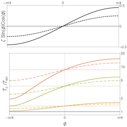
Figure 2: (Color online) Above: HEC of the state (8) as a function of $\phi$ for purity parameter $\zeta=\{0.9,0.5,0\}$ (solid, dashed, dotted). Below: ratio between cavity field temperature $T_{c}$ and the temperature of its local environment at $T_{\text{en}}$. Relative interaction strength $\mu_{c}/\kappa$ =$\{0,0.1,1,3\}$ (blue, orange, green, red). Average thermal photon number is $\bar{n}_{\text{en}}=0.1$, which could correspond to $T_{\text{en}}\sim$ mK ($\sim 298$ K) at microwave (optical) frequencies.                                                      

III Spectral measurements

Up to this point, we have verified that changes in the parameters controlling the HECs or in the size of the cluster have a direct impact on the temperature and thermalization time of the corresponding probe. Now, we present a way to experimentally test such predictions. In this section, we will address such an inquiry using the power spectrum of the probe.

Stationary power spectrum

The stationary (Wiener-Khintchine) power spectrum Wiener (1930); Khintchine (1934) associated with the single-qubit probe, is defined as (Carmichael, 1993; Castro-Beltrán et al., 2016):

$$S_{q}(\omega)=\frac{1}{\pi}{\rm Re}\int_{0}^{\infty}d\tau e^{i\omega\tau}\langle\sigma_{+}(0)\sigma_{-}(\tau)\rangle,$$ (10)

where $\langle\sigma_{+}(0)\sigma_{-}(\tau)\rangle\!=\!\lim_{t\rightarrow\infty}\langle\sigma_{+}(t)\sigma_{-}(t+\tau)\rangle$ is the first order dipole-field auto-correlation function. In the steady state of the system at hand, it can be calculated as (see Appendix B): $\langle\sigma_{+}(0)\sigma_{-}(\tau)\rangle\!=\!\rho_{ee}^{st}\exp[-(i\omega_{q}+\gamma_{\phi}+(2t_{q})^{-1})\tau]$. Using this result, we can perform the integral in Eq. (10) and obtain the stationary power spectrum of the qubit as follows

$$S_{q}(\omega)=\frac{\rho_{ee}^{st}}{\pi}\frac{\frac{1}{2}\Gamma_{q}}{\big{(}\omega-\omega_{q}\big{)}^{2}+\big{(}\frac{1}{2}\Gamma_{q}\big{)}^{2}},$$ (11)

which is a Lorentzian peak of full width at half maximum (FWHM) given by $\Gamma_{q}=2\gamma_{\phi}+t_{q}^{-1}$. Further, we can use Eq. (5) to replace the thermalization time and obtain

$$\Gamma_{q}=2\gamma_{\phi}+\gamma(2\bar{n}_{\rm en}+1)+2\mu_{q}(\langle J^{2}\rangle-\langle J_{z}^{2}\rangle).$$ (12)

$S_{q}(\omega)$ has a maximum at $\omega_{q}$ given by $2\rho_{ee}^{st}/(\Gamma_{q}\pi)$. The intensity can be calculated as the integral over all frequencies $I_{q}\equiv\int_{-\infty}^{\infty}S_{q}(\omega)d\omega=\rho_{ee}^{st}$. It is important to note that, since it is equal to the excited state population, any value of the intensity that is greater than $1/2$ indicates that the probe temperature has attained negative values.

On the other hand, the power spectrum of the single-field mode is defined as

$$S_{c}(\omega)=\frac{1}{\pi}{\rm Re}\int_{0}^{\infty}d\tau e^{i\omega\tau}\langle a^{\dagger}(0)a(\tau)\rangle,$$ (13)

and if we repeat the same procedure as we did for the qubit case, it is possible to find the power spectrum as

$$S_{c}(\omega)=\frac{n_{st}}{\pi}\frac{\frac{1}{2}\Gamma_{c}}{\big{(}\omega-\omega_{c}\big{)}^{2}+\big{(}\frac{1}{2}\Gamma_{c}\big{)}^{2}},$$ (14)

with its maximum and spectral bandwidth being $S_{c}(\omega_{c})=2n_{st}/(\Gamma_{c}\pi)$ and $\Gamma_{c}=2\kappa_{\phi}+t_{c}^{-1}$, respectively. Again, similar to the qubit case, we can substitute the thermalization time of the cavity from Eq. (7) to obtain

$$\Gamma_{c}=2\kappa_{\phi}+\kappa-2\mu_{c}\langle J_{z}\rangle,$$ (15)

resulting in a cavity intensity of $I_{c}\equiv\int_{-\infty}^{\infty}S_{c}(\omega)d\omega=n_{st}$. We observe that in both cases the spectral bandwidth depends explicitly on the corresponding thermalization times. Hence, by measuring the FWHM of these spectral signals, it is possible to infer how fast or slow is the thermalization process. Moreover, measuring their intensity (signal integration) one can obtain the apparent temperature that has been reached by the quantum probe.

If we rewrite the ratio $r_{d}/r_{e}$ ($\mathcal{R}_{d}/\mathcal{R}_{e}$) and the sum (difference) $r_{d}+r_{e}$ ($\mathcal{R}_{d}-\mathcal{R}_{e}$) in terms of $I_{q}$ ($I_{c}$) and $\Gamma_{q}$ ($\Gamma_{c}$) respectively, we can arrange simple and general expressions for the average values we are interested in:

$$\langle J_{+}J_{-}\rangle =(\Gamma_{\text{p}}-2\gamma^{\phi}_{\text{p}})({I}_{\text{p}})\mu_{\text{p}}^{-1}-\frac{\gamma_{\text{p}}}{\mu_{\text{p}}}\bar{n}_{\rm en},$$ (16a)

$$\langle J_{-}J_{+}\rangle =(\Gamma_{\text{p}}-2\gamma_{\text{p}}^{\phi})(1\pm{I}_{\text{p}})\mu_{\text{p}}^{-1}-\frac{\gamma_{\text{p}}}{\mu_{\text{p}}}(1+\bar{n}_{\rm en}),$$ (16b)

where the subscript “p” specify the type of the probe, i.e., $q$ or $c$. In the same manner, decay rate $\gamma_{\text{p}}$ ($\gamma_{\text{p}}^{\phi}$) must be replaced by $\gamma$ or $\kappa$ ($\gamma_{\phi}$ or $\kappa_{\phi}$). The change of sign in Eq. (16a) comes from considering the single-qubit instead of the cavity mode as the central system. Eqs. (16) are useful because they enable, together with some previous knowledge of the bath state like Eq. (9), to establish a link between spectroscopic parameters, $\Gamma_{\text{p}}$ and $I_{\text{p}}$ and HECs, therefore provide the information on whether or not HECs are present in the environment that our probe system is interacting. As the collective spin correlators carry information on the multipartite coherences and entanglement among the environment qubits, our results could allow for spectroscopic quantum thermometry of quantum correlations in a non-thermal environment that can be associated with an apparent temperature. In the following subsection, we will elaborate on these results.

Heat exange coherences in the power spectrum

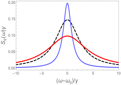
Figure 3: (Color online) Power spectrum of the single-qubit probe [see Eq. (11)] when the initial state of the environmental cluster is the Eq. (8). Black dashed line is for $\zeta=0$ (mix state). Solid lines are for $\zeta=0.9$ (state with HECs) and $\phi=\{-\pi/4,\pi/4\}$ (blue, red) represent, respectively, the coldest and hottest effective qubit temperature for this value of $\zeta$. We set $\mu_{q}=2\gamma$, $\gamma_{\phi}=0.15\gamma$ and $\bar{n}_{\rm en}=0.1$. The spectral bandwidth and the amplitude have a strong dependency on $\zeta$ and $\phi$.                                                                  

Now we use the spectra of Eqs. (11) and (14) to show how it is possible to differentiate between states of the $N$-qubit cluster having HECs from those who are a statistical mixture. For clarity we consider again the state described by Eq. (8) as an example, from Eq. (12) follows

$$\Gamma_{q}=2\gamma_{\phi}+\gamma(2\bar{n}_{\text{en}}+1)+2\mu_{q}(1+\zeta\sin 2\phi).$$ (17)

The inclusion of HECs in Eq. (8) will (depending on the sign of $\sin 2\phi$) increase or decrease the spectral bandwidth by an amount $\Delta\Gamma_{q}\equiv\Gamma_{q}-\Gamma_{q}^{\prime}=2\zeta\mu_{q}\sin 2\phi$, where $\Gamma_{q}^{\prime}$ is the FWHM of the mix state $\rho_{\rm cl}(\phi,0)$. The increase (decrease) is maximum when $\zeta=1$ and $\phi=\pi/4$ ($-\pi/4$). For $\phi=-\pi/4$ the bandwidth can even be equal to the natural (or fabricated) spectral linewidth of the qubit as long as $\gamma_{\phi}$ and $\bar{n}_{\rm en}$ are negligible. This behavior is shown in Fig. 3 where amplitude variations also can be observed. For the field mode case we cannot apply previous spectral bandwidth analysis when using Eq. (8) because $\langle J_{z}\rangle=0$ and $\Gamma_{c}=2\kappa_{\phi}+\kappa$ remains as if there had not been an interaction with the $N$-qubit cluster. However, signatures of HECs in $S_{c}(\omega)$ still can be found, these are encoded in the field intensity given by $I_{c}=\bar{n}_{\rm en}+(\mu_{c}/\kappa)(1+\zeta\sin 2\phi)$. Note that in both cases, HECs affect the same spectral parameters that the temperature of the thermal environment affects. This is in line with our claims that HECs only contribute to the heat flow between the interacting quantum probe and non-thermal environment but cannot be transferred as coherence. All in all, it is nice to see this verification in experimentally accesible spectroscopic parameters.

On the other hand, if the cluster is initially in the Dicke state $|k,N\rangle$ with $k=N/2-1$, then the bandwidth of the single-qubit central system depends quadratically on $N$:

$$\Gamma_{\text{Dicke}}=2\gamma_{\phi}+\gamma(2\bar{n}_{\rm en}+1)+\mu_{q}(N+N^{2}/2-2).$$ (18)

Thus, in this case, given a set of values $\{\gamma_{\phi},\gamma,\bar{n}_{\rm en}\}$ there should be a critical number of qubits in the cluster in order to be more significant than contributions of the dissipation and/or dephasing rate. In other words, the control of the spectral bandwidth is imposed by changes of the cluster size.

These results indicate that, with some previous information of the bath state like Eq. (9), we are capable of discriminating between a quantum non-thermal machine operating with a bath containing HECs, from a thermal machine in which its environment is in a mixed state. Even more, we can know if the associated probe temperature is increasing or decreasing together with its rate, just by looking at the spectral properties of it. In fact, presented approach is quite similar to the one put forward in Razavian et al. (2019), in which the authors suggest to assess the temperature of an environment by looking at the dephasing dynamics of a single, probe qubit that is in contact with that environment. In other words, even though the type of the environment and the interaction with the probe qubit is quite different in the model we consider as compared to Razavian et al. (2019), the power spectrum of the probe can be used in the same spirit, that is, to estimate the apparent temperature of its environment. However, in this work, the environment that the probe qubit is in contact with do not need to be a thermal one, it can also be a non-thermal, coherent one that dictates an apparent temperature to the probe, through HECs.

Experimental measurements of previous results will be limited by the resolution of the power spectrum Clerk et al. (2010); Tsang et al. (2011) and hence errors in the FWHM and in the intensity would propagate to the errors in coherence and in the apparent temperature respectively. As the errors in power spectrum measurements may arise from technical/systematic errors as well, we ask, more fundamentally, general bounds on estimating the apparent temperature and the HECs of the non-thermal bath by conventional quantum thermometry Stace (2010); Pasquale and Stace (2018); Mehboudi et al. (2019) and estimation theory Jing et al. (2014).

To determine the ultimate limit for which the apparent temperature $T_{p}$ of our quantum probes (qubit or cavity) can be estimated, we need to resort to the quantum Cramér-Rao bound which reads as Mehboudi et al. (2019) $\Delta T_{p}\geq 1/\sqrt{\nu\mathcal{F}(\rho_{p})}$, where $\nu$ is the number of independent measurements and $\mathcal{F}(\rho_{p})$ is the quantum Fisher information (QFI) of the state $\rho_{p}$, the latter depends on the parameter $T_{p}$ that we want to estimate. When the state of the probe is a thermal state the QFI can be written in terms of the variance of the probe Hamiltonian as Correa et al. (2015) $\mathcal{F}(\rho_{p})=(\Delta H_{p})^{2}/(k_{B}^{2}T_{p}^{4})$. Precisely, the steady state solutions of both Eq. (1) and Eq. (6) are thermal states $\rho_{p}^{st}=\exp(-H_{p}/k_{B}T_{p})Z^{-1}$ with $Z$ being the corresponding partition function. Following Ref. Campbell et al. (2018), QFI of the qubit probe and the field probe (harmonic oscillator), at the steady state, are given by $\mathcal{F}(\rho_{q}^{st})=\big{(}{\hbar\omega_{q}}/{2k_{B}T_{q}^{2}}\big{)}^{2}{\rm sech}^{2}\big{(}{\hbar\omega_{q}}/{2k_{B}T_{q}}\big{)}$ and $\mathcal{F}(\rho_{c}^{st})=\big{(}{\hbar\omega_{c}}/{2k_{B}T_{c}^{2}}\big{)}^{2}{\rm csch}^{2}\big{(}{\hbar\omega_{c}}/{2k_{B}T_{c}}\big{)}$ respectively. We present the behaviors of these quantities in Fig. 4.

It is possible to conclude that, for a fixed energy gap of the probe, both probes estimate a specific apparent temperature with a higher precision than other temperatures. That specific value of the apparent temperature corresponding to the maximum of the QFI is linearly related with the energy level splitting of the probe, this is $2k_{B}T_{p}^{\rm max}=\alpha_{p}\hbar\omega_{p}$, where $\alpha_{p}$ satisfies the transcendental equations Campbell et al. (2018): $2\alpha_{q}=\tanh(\alpha_{q}^{-1})$ for the qubit probe and $2\alpha_{c}=\coth(\alpha_{c}^{-1})$ for the cavity probe. These two transcendental equations have an approximate solution $\alpha_{p}\approx 0.5$ ($\alpha_{q}=0.484$ and $\alpha_{c}=0.522$ exactly) that can be inferred, roughly, from their behaviour in Fig. 4. Thus, the apparent temperature which can be estimated with the maximum precision (the minimum uncertainty $\Delta T_{p}$) is $T_{p}^{\rm max}\sim\hbar\omega_{p}/4k_{B}$.

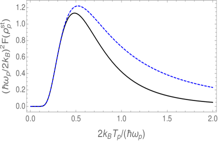
Figure 4: Quantum Fisher information of each quantum probe. Solid-black (blue-dashed) line is for the qubit (cavity) probe.                                                                 

In the present scheme, since the apparent temperature is inherently dependent on the value of HECs in the bath, it is also possible to extend the usage of the above information and determine how precisely one can identify the amount of HECs in the bath state. However, to obtain the uncertainty of the HECs from the uncertainty on the apparent temperature, a proper error propagation treatment should be done. Instead, we reproduce the parameter estimation framework of Mehboudi et al. (2019) and Jing et al. (2014) but focusing directly on $\zeta$ (the purity or amplitude parameter in the HECs of the state (8)) rather than the apparent temperature. Since $T_{p}=T_{p}(\zeta)$, the probabilities $p_{n}\equiv\langle\epsilon_{n}|\rho_{p}^{st}|\epsilon_{n}\rangle$ which depend on $T_{p}$ will also depend on $\zeta$, i.e., $p_{n}=p_{n}(T_{p}(\zeta))$, here $|\epsilon_{n}\rangle$ is an eigenstate of $H_{p}$. Following very closely Mehboudi et al. (2019); Jing et al. (2014) and making use of the chain rule $\partial p_{n}/\partial\zeta=(\partial p_{n}/\partial T_{p})(\partial T_{p}/\partial\zeta)$, it is possible to get a compact and simple form of the QFI associated with the estimation of $\zeta$, in terms of the QFI for thermal states of the probe times the rate of change of the apparent temperature with respecto to $\zeta$:

$$\mathcal{F}(\rho_{\zeta})=\mathcal{F}(\rho_{p}^{st})(\partial T_{p}/\partial\zeta)^{2}.$$ (19)

Due to the general form of the above expression, it can be used to estimate any other parameter that is linked with the apparent temperature, such as the phase of the HECs for instance. Using the expression of the apparent temperature for the qubit probe the Eq. (19) can be written, in a more explicit form, in terms of the heating and cooling rates

$$\mathcal{F}(\rho_{\zeta})=\frac{r_{e}}{r_{d}}\left[\left(\frac{r_{e}}{r_{e}+r_{d}}\right)\frac{\partial}{\partial\zeta}\left(\frac{r_{d}}{r_{e}}\right)\right]^{2}.$$ (20)

Therefore, the uncertainty in the estimation of $\zeta$ will be bounded by $\Delta\zeta\geq 1/\sqrt{\nu\mathcal{F}(\rho_{\zeta})}$. One can take a step further and give an explicit expression for the $\mathcal{F}(\rho_{\zeta})$ for the state given in Eq. (8) as follows

$$\mathcal{F}(\rho_{\zeta})=\frac{(\mu_{q}/\gamma)^{2}\sin^{2}(2\phi)}{z(1+z)(1+2z)^{2}},$$ (21)

where $z=\bar{n}_{\rm en}+(\mu_{q}/\gamma)(1+\zeta\sin 2\phi)$.

IV Displacement coherences in the power spectrum

We now want to shift our attention from HECs to the different class of coherences in $\rho_{\rm cl}$ and analyze their effect on the power spectrum of the single qubit probe. In particular, we present how it is possible to shape the spectrum using the so called displacement coherences (DCs) Manatuly et al. (2019), which are the matrix elements of $\rho_{\rm cl}$ that contribute to the expectation values $\langle J_{\pm}\rangle$ Dağ et al. (2016); Çakmak et al. (2017). Under the assumptions outlined in Sec. II.1, we can obtain an equation that rules the evolution of the single qubit probe assuming that only DCs are present in the coherent atomic cluster. Up to second order in $g\texttt{t}$ the equation describing the dynamics reads as (see Appendix A for details):

$$\dot{\rho}_{q}=-i[H_{\rm eff},\rho_{q}],$$ (22)

where

$$H_{\rm eff}=\tilde{\mu}\langle J_{+}\rangle\sigma_{-}+\tilde{\mu}\langle J_{-}\rangle\sigma_{+}$$ (23)

is the effective Hamiltonian. Note that $H_{\rm eff}$ emulates the semi-classical radiation-matter interaction between a two-level atomic system and a classical electric field. It is possible to identify an effective Rabi frequency given by $\Omega_{\rm eff}=2\tilde{\mu}|\langle J_{\pm}\rangle|$ with $\tilde{\mu}=pg\texttt{t}$. In order to clearly and explicitly present the action of DCs on the spectrum of the qubit probe, we set $\gamma=\gamma_{\phi}=\bar{n}_{\rm en}=0$, $\langle J_{\pm}^{2}\rangle=\langle J_{\pm}J_{\mp}\rangle=0$, and keep only $\langle J_{\pm}\rangle\neq 0$ which guarantees that atomic bath clusters contain only DCs.

Since Eq. (22) describes unitary evolution of the system, it does not present a steady-state solution and thus we cannot make use of the quantum-regression formula to compute the dipole-field autocorrelation function. Therefore, it is not possible to calculate the idealized stationary power spectrum definition presented in Eq. (10). Instead, we will use the physical spectrum introduced by Eberly and Wódkiewicz (EW) Eberly and Wódkiewicz (1977). In general, this spectrum definiton can be applied to non-stationary light sources. For the single qubit probe it is defined as:

$$S(\omega,t,\Gamma_{\rm f})=2\Gamma_{\rm f} \int_{0}^{t}dt_{1}\int_{0}^{t}dt_{2}e^{-(\Gamma_{\rm f}-i\omega)(t-t_{1})}$$

$$\times e^{-(\Gamma_{\rm f}+i\omega)(t-t_{2})}\langle\sigma_{+}(t_{1})\sigma_{-}(t_{2})\rangle,$$ (24)

where $\omega$ and $\Gamma_{\rm f}$ are the central frequency and band half-width of a Fabry-Pérot cavity acting as a filter, respectively, and we assume its central line matches the qubit frequency $\omega_{q}$. The EW-spectrum is more realistic, it reduces to the previously introduced definition by Wiener-Khintchine for the stationary state, $t\rightarrow\infty$, and in the limit of infinite resolution, $\Gamma_{\rm f}\rightarrow 0$ Eberly and Wódkiewicz (1977). If the qubit probe is initially in its ground state the dipole-field auto-correlation function is easily obtained [see Eq. (B)], and we can use it to express Eq. (IV) in following way

$$S(\omega,t,\Gamma_{\rm f})= \frac{\Gamma}{2}e^{-2\Gamma_{\rm f}t}\Big{\{}\Big{|}\int_{0}^{t}d\tau e^{(\Gamma_{\rm f}-i\omega)\tau}\sin(\Omega_{\rm eff}\tau)\Big{|}^{2}$$

$$+ \Big{|}\int_{0}^{t}d\tau e^{(\Gamma_{\rm f}-i\omega)\tau}\big{[}1-\cos(\Omega_{\rm eff}\tau)\big{]}\Big{|}^{2}\Big{\}}.$$ (25)

Analytical solution for the integrals of Eq. (IV) is possible, however, the entire expression of the full time-dependent spectrum is too cumbersome to show here. Instead, a good approximate time-independent expression can be obtained in the long-time limit ($t\gg 1$) Román-Ancheyta et al. (2018), where after a few Rabi oscillations the spectrum has stabilized to three nearby Lorentzians:

$$S(\omega,\Gamma_{\rm f})= \frac{\frac{1}{4}\Gamma_{\rm f}}{\Gamma_{\rm f}^{2}+[(\omega-\omega_{q})+\Omega_{\rm eff}]^{2}}+\frac{\frac{1}{2}\Gamma_{\rm f}}{\Gamma_{\rm f}^{2}+(\omega-\omega_{q})^{2}}$$

$$+\frac{\frac{1}{4}\Gamma_{\rm f}}{\Gamma_{\rm f}^{2}+[(\omega-\omega_{q})-\Omega_{\rm eff}]^{2}}.$$ (26)

A Mollow-like structure Mollow (1969) can be inferred from above expression and its explicit behavior is shown in Fig. 5, where the satellite peaks are located at $\omega=\omega_{q}\pm\Omega_{\rm eff}$. Recall that $\Omega_{\rm eff}$ is directly proportional to $\langle J_{\pm}\rangle$, therefore the magnitude of the DCs defines if the single qubit probe is in the weak, moderate or strong (where the sidebands emerge) driven regime. If we add energy losses into our system, we will be simulating the physical process of resonance fluorescence (RF) with an exact Mollow spectrum as a final result Mollow (1969). Such a setting can be created within the framework of the model we present in this work.

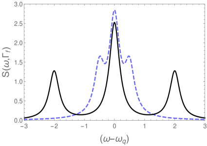
Figure 5: Spectrum the the single qubit probe (IV) when displacement coherences of the $N$-qubit cluster are taken into account. The displacement coherences, $\langle J_{\pm}\rangle$, define the location of the sidebands in this Molow-like spectrum. We have set the effective Rabi frequency $\Omega_{\rm eff}\equiv 2\tilde{\mu}|\langle J_{\pm}\rangle|$ equals to 2 (black solid line) and 1/2 (blue dashed line). $\Gamma_{\rm f}=0.2$.          

A motivation to study the Mollow spectrum of RF in the suggested configuration, is due to the fact that this has became in a figure of merit for the coherent manipulation of semiconductors quantum dots Muller et al. (2007) and superconducting qubits Astafiev et al. (2010). We also think that suggested setups are more practical as compared to cavity-QED configurations, in particular, they can be implemented in compact solid-state architectures, where no laser light and/or three-dimensional electromagnetic cavities are need. However, depending on the experimental implementation, unless we prepare the DCs with a well-define phase reference they will cancel out, on average, after each sequential cluster-probe interaction Latune et al. (2019). These operational difficulties can be mitigated by reducing the number of qubits involved in the cluster. Actually, we only need just one qubit with DCs in order to perform the quantum simulation of resonance fluorescence, however, the corresponding Rabi frequency that one can obtain in such configuration will be small one and maybe hard to distinguish from the central peak. Similarly, choosing a cluster with a minimum size of two-qubits, and assuming that all different types of coherences are present in the non-thermal bath, i.e. $\langle J_{\pm}\rangle$, $\langle J_{\pm}^{2}\rangle$ and $\langle J_{\pm}J_{\mp}\rangle$ are different from zero, then we could perform the quantum simulation of RF from a single two-level system in an artificial squeezed vacuum by a repeated interaction scheme. This scheme generates an effective Markovian master equation (A) identical to that of a driven two-level atom in a squeezed vacuum in free space, without the necessity to use sources of true squeezed light. As the scheme consists of only qubit-qubit interactions it can provide arbitrarily strong squeezing Dağ et al. (2016). Therefore, this is a viable alternative to control polarization decay and spectral response of a single qubit probe. Notice that we do not have to wait for the steady state solution driven by a large number of repeated interactions or collisions. Equation (IV) is valid, in general, for non-stationary sources of light. This means that with just a few number of collisions between the quantum probe and the small coherent clusters, which means a short evolution, the time-dependent spectrum could be, in principle, measured. Actually, in Román-Ancheyta et al. (2018) one of us proved that after just a few Rabi oscillations, a well-define Mollow-like spectrum can be obtained using Eq. (IV).

In addition to spectrum engineering and longevity of quantum coherence, these results can be significant for spectral characterization of unknown quantum resources for their quantum information and energy resource values as well. From the quantum thermodynamic point of view, the emergence of a Mollow-like triplet in the spectroscopy of the corresponding qubit probe should be considered as a strong signature of the system acting as a thermo-mechanical engine, such that the interaction with the non-thermal bath result in both heat and work to be imparted to the probe Dağ et al. (2016).

V Experimental relevance

In this section, we would like to elaborate on the experimental side of our motivation to use the power spectrum to determine the apparent temperature of the quantum probe and, ultimately, the apparent temperature of the non-thermal bath.

As we have discussed in Sec.s II.1 and II.2, the apparent temperature of the probe can be determined by the excited state population and the mean number of photons at the steady state, respectively. Extracting this information from the power spectra of the probes are in fact possible by looking at the integral of the spectra over all frequencies, i.e. their intensities, as shown in Sec. III. With this knowledge at hand, there are two relevant experimental works performing the so called fluorescence thermometry of thermal baths using a single quantum dot Haupt et al. (2014) and nitrogen-vacancy (NV) centres in diamond nanocrystals (nanodiamonds) Kucsko et al. (2013). In both cases the fluorescence of the quantum thermometer is converted to population measurements, which is in line with the discussion we made above. Apart from the fact that we study quantum thermometry of non-thermal baths, one of the main differences between Ref.s Haupt et al. (2014); Kucsko et al. (2013) and our work is that we are considering only spinless quantum probes. For example, in Haupt et al. (2014) the ultra-cold temperature of the quantum dot is extracted by combining, the Fermi-Dirac distribution and the relative amplitudes of the absorption resonance for the high-energy and low-energy optical transitions (see Eq. (1) of Haupt et al. (2014)). Moreover, in quite contrast with our work, the precise value of the transition frequency between the ground state and the two-degenerate excited states of the NV-centres, has a temperature dependence due to thermally induced lattice strains. Therefore, the operational principle of this quantum thermometer relies on the accurate measurement of such transition frequency, which can be done with high spatial nanometer resolution Kucsko et al. (2013). In our work, the corresponding transition frequencies of the quantum probes do not depend on the temperature.

Regarding the issue of which technique could be used experimentally to determine the probe power spectrum, we would like to emphasize that our results are general and depending on the specific experimental implementation of the setup, the power spectrum should be measured in the appropriate context. For instance, if our scheme is implemented in a circuit-QED architecture, one should record the resonator transmission spectrum using a continuous-wave measurement at low drive Blais et al. (2004), where the transmission frequencies are spectrally resolved in a heterodyne detection scheme Fink et al. (2008). Actually, in the linear response limit the drive term can be neglected from the coherent dynamics Fink et al. (2010), which is really useful for the numerical calculation of the transmission spectrum. On the other hand, if our scheme is implemented in a cavity-QED setup, the fluorescence spectrum of the quantum probe could be measured using, for example, the standard balance homodyne detection schemes Castro-Beltrán et al. (2016). In this technique the phase of the unknown signal is measured by mixing it with a strong local oscillator (LO) in a beam splitter, where the LO is a field with a well-define amplitude and phase. Using a spectrum analyzer, the output intensity from each beam splitter ports are subtracted electronically and the desired signal is obtained as a result, which is proportional to the amplitude of the quantum field Gerry and Knight (2004).

Another field of research that experimental assessment of the apparent temperature of quantum systems is highly relevant are quantum Hall systems. The topological order of some fractional quantum Hall states are better characterized by the thermal Hall conductance, which is a topological invariant and therefore has quantized values Banerjee et al. (2017, 2018); Ma and Feldman (2019). It is possible to distinguish between Abelian and non-Abelian states of matter by identifying if the thermal Hall conductance is quantized to integer and non-integer values, respectively. The latter case opens up the possibility of using these systems for braiding of non-Abelian particles which is beneficial for topological quantum computing. However, precise determination of thermal Hall conductance requires precise information on the temperature of the state. We hope that the scheme presented in the present work can contribute along these lines.

VI Conclusions

We have studied the thermalization dynamics of two different types of quantum probes that are in contact with a thermal and non-thermal, coherent bath. We have modeled our quantum probes as a single-qubit and a single-mode cavity field, and showed the non-trivial effects of the coherences contained in the non-thermal bath (HECs) on the thermalization temperature and time of these model systems. We have proposed a strategy to measure these effects by investigating the power spectrum of the probes in both cases, and proved that the spectral bandwidth and intensity are explicitly dependent on HECs. Therefore, the suggested method is capable of identifying the apparent temperature of a non-thermal bath with HECs, as well as the temperature of a thermal bath, in spectroscopic experiments. We think that these results also contribute to the field of quantum thermometry which aims to estimate the temperature of an environment using a quantum probe. The presented spectroscopic method is not only capable of assessing the temperature of a thermal bath, but also points a direction on how to identify the apparent temperature (positive and negative) that a quantum probe sees when in contact with an non-thermal environment with only thermalizing coherences. Through such an apparent temperature, quantum thermometry of multipartite coherences and correlations could be possible for non-thermal environments. Another application of this method is the implementation of quantum simulation of resonance fluorescence using different types of coherences in the non-thermal bath. On top of being an significant result per se, observation of such an effect can again serve as a tool for characterizing an unknown environment via a single-qubit probe. Even though the presented repeated interaction scheme may present some practical challenges at the implementation stage, for example the preparation or re-initialization of the coherent cluster, we hope that the results presented in this work can further induce investigations on non-thermal baths through spectral measurements of a probe system.

Appendix A Generalized micromaser like equation

We make the derivation, following closely Ref. Liao et al. (2010), of the micromaser master like equation used in Eqs. (1) and (6) of the main text. We start by considering a “multipulse” type interaction between a central system $S$ and a bath system $B$ that is described by the linear coupling Hamiltonian $H_{I}=\epsilon(B^{\dagger}s+Bs^{\dagger})$, where $s,s^{\dagger}$ ($B,B^{\dagger}$) are the annihilation and creation, central (bath) system operators respectively; $\epsilon$ is the coupling coefficient. The corresponding evolution operator is $U(\tau)=\exp(-iH_{I}\tau)$. Before each interaction at time $t_{j}$, it is assumed that the state of the bath system $B$ is reset to its initial value which does not have any correlation with $S$, so the total state is $\rho(t_{j})=\rho_{\text{\tiny S}}(t_{j})\otimes\rho_{\text{\tiny B}}(0)$. This assumption seems arbitrary, but actually, it is a typical physical situation in one-atom masers Filipowicz et al. (1986) for which, individual and independent Rydberg atoms pass one by one through a high-finesse electromagnetic cavity Meschede et al. (1985); Rempe et al. (1987, 1990). After each interaction of duration $\tau$, the central system density matrix is $\rho_{\text{\tiny S}}(t_{j}+\tau)=\text{Tr}_{\text{\tiny B}}\{U(\tau)\rho(t_{j})U^{\dagger}(\tau)\}$. If we introduce a rate $p$ of a Poisson process to portray this interaction, then in a time interval $(t+\delta t)$ the probability of interaction will be $p\delta t$. As a consequence the state of the central system $S$ can be written during this time interval as the sum of the two possible outcomes $\rho_{\text{\tiny S}}(t+\delta t)=p\delta t\text{Tr}_{\text{\tiny B}}{\{}U(\tau)\rho(t)U^{\dagger}(\tau){\}}+(1-p\delta t)\rho_{\text{\tiny S}}(t)$, where $1-p\delta t$ is the probability of having a non interaction event. If we divided the above equation by $\delta t$ and take the limit when it goes to zero, we obtain the following differential equation for the central system density matrix

$$\dot{\rho}_{\text{\tiny S}}(t)=p\big{[}{\rm Tr}_{\text{\tiny B}}\{U(\tau)\rho_{\text{\tiny S}}(t)\otimes\rho_{\text{\tiny B}}(0)U^{\dagger}(\tau)\}-\rho_{\text{\tiny S}}(t)\big{]},$$ (27)

where we have used the derivative definition: $\text{d}\rho_{\text{\tiny S}}(t)/\text{d}t\equiv\lim_{\delta t\rightarrow 0}\left(\rho_{\text{\tiny S}}(t+\delta t)-\rho_{\text{\tiny S}}(t)\right)/\delta t$. By now (27) is valid for any coupling strength and interaction time, however, in micromaser setups the product $\epsilon\tau$ is normally small Liao et al. (2010). We proceed to approximate the evolution operator up second order in $\epsilon\tau$ as: $U(\tau)\sim 1-U_{1}(\tau)-U_{2}(\tau)$, where

$$U_{1}(\tau) =i\epsilon\tau(B^{\dagger}s+Bs^{\dagger}),$$ (28)

$$U_{2}(\tau) ={(\epsilon\tau)}^{2}(B^{\dagger}s+Bs^{\dagger})^{2}/2.$$ (29)

Inserting (28), (29) in (27), it yields

$$\dot{\rho}_{\text{\tiny S}}(t)=p {\rm Tr}_{\text{\tiny B}}\big{\{}U_{1}(\tau)\rho(t)U_{1}^{\dagger}(\tau)-U_{1}(\tau)\rho(t)$$

$$-\rho(t)U_{1}^{\dagger}(\tau)-U_{2}(\tau)\rho(t)-\rho(t)U_{2}^{\dagger}(\tau)\big{\}},$$ (30)

where we have kept only terms up second order in $\epsilon\tau$ neglecting $U_{1}(\tau)\rho(t)U_{2}^{\dagger}(\tau)\propto(\epsilon\tau)^{3}$, $U_{2}(\tau)\rho(t)U_{2}^{\dagger}(\tau)\propto(\epsilon\tau)^{4}$ and their complex conjugates. Hereafter we denote $\rho_{\text{\tiny S}}(t)$ as $\rho_{\text{\tiny S}}$. Tracing out of the bath degrees of freedom in (A) we obtain the following micromaser master like equation

$$\dot{\rho}_{\text{\tiny S}}=-i [H_{\rm eff},\rho_{\text{\tiny S}}]+\frac{\mu}{2}\langle BB^{\dagger}\rangle\mathcal{L}[s]\rho_{\text{\tiny S}}+\frac{\mu}{2}\langle B^{\dagger}B\rangle\mathcal{L}[s^{\dagger}]\rho_{\text{\tiny S}}$$

$$+ \frac{\mu}{2}\langle B^{2}\rangle\mathcal{L}_{\text{{\tiny S}q}}[s^{\dagger}]\rho_{\text{\tiny S}}+\frac{\mu}{2}\langle B^{\dagger 2}\rangle\mathcal{L}_{\text{{\tiny S}q}}[s]\rho_{\text{\tiny S}},$$ (31)

where $\mu=p(\epsilon\tau)^{2}$ and $H_{\rm eff}=p\epsilon\tau(\langle B^{\dagger}\rangle s+\langle B\rangle s^{\dagger})$. The average values are taken with respect to the initial bath state, i.e., $\langle\mathcal{O}\rangle={\rm Tr}\{\rho_{\text{\tiny B}}(0)\mathcal{O}\}$. The Lindblad superoperators are defined as: $\mathcal{L}[o]\rho_{\text{\tiny S}}\equiv 2o\rho_{\text{\tiny S}}{o^{\dagger}}-{o^{\dagger}}{o}\rho_{\text{\tiny S}}-\rho_{\text{\tiny S}}{o^{\dagger}}{o}$ and $\mathcal{L}_{\text{{\tiny S}q}}[{o}]\rho_{\text{\tiny S}}\equiv 2{o}\rho_{\text{\tiny S}}{o}-{o}^{2}\rho_{\text{\tiny S}}-\rho_{\text{\tiny S}}{o}^{2}$. During the derivation of (A) it was not necessary to specify if system $S$ and/or $B$ were from a bosonic or fermionic nature. Moreover, no restrictions have been made regarding their composition, $S$ and $B$ can represent either individual quantum systems or several non-interacting ones. As long as their interaction Hamiltonian can be written in the form of $H_{I}$ together with the previous assumptions, (A) will be valid.

It was assumed that between each interaction the central system $S$ evolves unitarily. However, it is possible that $S$ could experience energy losses and/or decoherence during the evolution due to the unavoidable interaction with its surrounding. In such a case, it easy to prove (see Ref. Liao et al. (2010)), within the approach of the theory of open quantum systems Carmichael (1993), that the only modification to (A) is to add another series of Lindbladians, $\propto\mathcal{L}_{j}[\mathcal{O}_{j}]\rho_{\text{\tiny S}}$, for each $j$ dissipation and/or dephasing process.

Equation (A) reduces to Eq. (1) [Eq. (6)] choosing $H_{I}$ as $H_{\text{dip}}$ ($H_{\text{TC}}$). In such case bath system $B$ would be the non interacting $N$-qubit coherent cluster and we replace $B$ by $J_{-}$. Central system $S$ will be the single-qubit (single cavity field mode) so that $s\rightarrow\sigma$ ($a$) and $\mu\rightarrow\mu_{q}$ ($\mu_{c}$). Additionally, we demand that $\rho_{\text{\tiny B}}(0)$ satisfy $\langle B\rangle=\langle B^{2}\rangle=0$ while $\langle B^{\dagger}B\rangle$ and $\langle BB^{\dagger}\rangle$ should be different from zero. On the other hand, if we allow only $\langle B\rangle$ and $\langle B^{\dagger}\rangle$ to survive, just the unitary part of (A) will remain, this is the condition to derive Eq. (22).

Eq. (A) is quite general and it is applicable to several micromaser based models Dağ et al. (2016); Çakmak et al. (2017); Dağ et al. (2019) including superradiant systems Hardal and Müstecaplıoğlu (2015) and entangled qubit environments Daryanoosh et al. (2018). Also it works for the case of generalized quantum “phaseonium fuels” Türkpençe and Müstecaplıoğlu (2016), where the bath system consists of a $N+1$ level atom with $N$ degenerate coherent ground states Türkpençe and Román-Ancheyta (2019). Unlike those previous works, (A) allows to get, more easily, analytical results.

Appendix B Autocorrelation functions

In the stationary case we know that $\langle\sigma_{+}(0)\sigma_{-}(\tau)\rangle$= $\lim_{t\rightarrow\infty}\langle\sigma_{+}(t)\sigma_{-}(t+\tau)\rangle$ is the first order dipole-field (${E}^{(+)}\propto\sigma_{-}$) autocorrelation function in the steady state. The quantum regression formula (QRF) allows us to obtain such two-time correlation from the single-time function $\langle\sigma_{-}(t)\rangle$ Carmichael (1993). Identifying that $\langle\sigma_{-}(t)\rangle=\rho_{eg}(t)$ and $\langle\sigma_{+}(t)\sigma_{-}(t)\rangle=\rho_{ee}(t)$, the use of the QRF in Eq. (2a) gives $\langle\sigma_{+}(t)\sigma_{-}(t$+$\tau)\rangle=\rho_{ee}(t)\exp[-(2\gamma_{\phi}+(2t_{q})^{-1})\tau]$; which in the steady state limit and in the Schrödinger picture yields

$$\langle\sigma_{+}(0)\sigma_{-}(\tau)\rangle=\rho_{ee}^{st}\exp[-(i\omega_{q}+2\gamma_{\phi}+(2t_{q})^{-1})\tau].$$ (32)

For the time-dependent case, the solution for the density matrix is $\rho_{q}(t)=U_{q}(t)\rho_{q}(0)U_{q}^{\dagger}(t)$, where $U_{q}(t)=\cos(t\Omega_{\rm eff}/2)-i\sigma_{x}\sin(t\Omega_{\rm eff}/2)$  Juárez-Amaro et al. (2015). Using $U_{q}(t)$ the dipole-field autocorrelation function for the qubit, starting in its ground state $\rho_{q}(0)=|g\rangle\langle g|$, is

$$\langle g|\sigma_{+}(t_{1})\sigma_{-}(t_{2})|g\rangle= \sin^{2}\big{(}t_{1}\Omega_{\rm eff}/2\big{)}\sin^{2}\big{(}t_{2}\Omega_{\rm eff}/2\big{)}$$

$$+ \sin\big{(}t_{1}\Omega_{\rm eff}\big{)}\sin\big{(}t_{2}\Omega_{\rm eff}\big{)}/4,$$ (33)

which we use in the integral of Eq. (IV) to obtain Eq. (IV).

References

- Vinjanampathy and Anders (2016) Sai Vinjanampathy and Janet Anders, “Quantum thermodynamics,” Contemporary Physics 57, 545–579 (2016).
- Goold et al. (2016) John Goold, Marcus Huber, Arnau Riera, Lídia del Rio, and Paul Skrzypczyk, “The role of quantum information in thermodynamics—a topical review,” Journal of Physics A: Mathematical and Theoretical 49, 143001 (2016).
- Alicki and Kosloff (2018) Robert Alicki and Ronnie Kosloff, “Introduction to quantum thermodynamics: History and prospects,” in Thermodynamics in the Quantum Regime: Fundamental Aspects and New Directions, edited by Felix Binder, Luis A. Correa, Christian Gogolin, Janet Anders, and Gerardo Adesso (Springer International Publishing, Cham, 2018) pp. 1–33.
- Deffner and Campbell (2019) Sebastian Deffner and Steve Campbell, Quantum Thermodynamics (Morgan & Claypool Publishers, 2019).
- Merali (2017) Zeeya Merali, “The new thermodynamics: how quantum physics is bending the rules,” Nature 551, 20–22 (2017).
- Scully (2002) Marlan O. Scully, “Extracting work from a single heat bath via vanishing quantum coherence ii: Microscopic model,” AIP Conference Proceedings 643, 83–91 (2002).
- Scully et al. (2003) Marlan O. Scully, M. Suhail Zubairy, Girish S. Agarwal, and Herbert Walther, “Extracting work from a single heat bath via vanishing quantum coherence,” Science 299, 862–864 (2003).
- Dağ et al. (2019) Ceren B. Dağ, Wolfgang Niedenzu, Fatih Ozaydin, Özgür E. Müstecaplıoğlu, and Gershon Kurizki, “Temperature control in dissipative cavities by entangled dimers,” The Journal of Physical Chemistry C 123, 4035–4043 (2019).
- Manatuly et al. (2019) Angsar Manatuly, Wolfgang Niedenzu, Ricardo Román-Ancheyta, Barış Çakmak, Özgür E. Müstecaplıoğlu, and Gershon Kurizki, “Collectively enhanced thermalization via multiqubit collisions,” Phys. Rev. E 99, 042145 (2019).
- Hardal and Müstecaplıoğlu (2015) Ali ÜC Hardal and Özgür E Müstecaplıoğlu, “Superradiant quantum heat engine,” Sci. Rep. 5, 12953 (2015).
- Türkpençe and Müstecaplıoğlu (2016) Deniz Türkpençe and Özgür E. Müstecaplıoğlu, “Quantum fuel with multilevel atomic coherence for ultrahigh specific work in a photonic carnot engine,” Phys. Rev. E 93, 012145 (2016).
- Quan et al. (2006) H. T. Quan, P. Zhang, and C. P. Sun, “Quantum-classical transition of photon-carnot engine induced by quantum decoherence,” Phys. Rev. E 73, 036122 (2006).
- Liao et al. (2010) Jie-Qiao Liao, H. Dong, and C. P. Sun, “Single-particle machine for quantum thermalization,” Phys. Rev. A 81, 052121 (2010).
- Dağ et al. (2016) Ceren B. Dağ, Wolfgang Niedenzu, Özgür E. Müstecaplıoğlu, and Gershon Kurizki, “Multiatom quantum coherences in micromasers as fuel for thermal and nonthermal machines,” Entropy 18, 244 (2016).
- Çakmak et al. (2017) B. Çakmak, A. Manatuly, and Ö. E. Müstecaplıoğlu, “Thermal production, protection, and heat exchange of quantum coherences,” Phys. Rev. A 96, 032117 (2017).
- Roßnagel et al. (2014) J. Roßnagel, O. Abah, F. Schmidt-Kaler, K. Singer, and E. Lutz, “Nanoscale heat engine beyond the carnot limit,” Phys. Rev. Lett. 112, 030602 (2014).
- Niedenzu et al. (2016) Wolfgang Niedenzu, David Gelbwaser-Klimovsky, Abraham G Kofman, and Gershon Kurizki, “On the operation of machines powered by quantum non-thermal baths,” New Journal of Physics 18, 083012 (2016).
- Niedenzu et al. (2018) Wolfgang Niedenzu, Victor Mukherjee, Arnab Ghosh, Abraham G. Kofman, and Gershon Kurizki, “Quantum engine efficiency bound beyond the second law of thermodynamics,” Nature Communications 9 (2018).
- Latune et al. (2019) C L Latune, I Sinayskiy, and F Petruccione, “Apparent temperature: demystifying the relation between quantum coherence, correlations, and heat flows,” Quantum Science and Technology 4, 025005 (2019).
- Alicki and Gelbwaser-Klimovsky (2015) Robert Alicki and David Gelbwaser-Klimovsky, “Non-equilibrium quantum heat machines,” New Journal of Physics 17, 115012 (2015).
- Alicki (2014) Robert Alicki, “Comment on “Nanoscale Heat Engine Beyond the Carnot Limit”,” arXiv e-prints , arXiv:1401.7865 (2014), arXiv:1401.7865 [quant-ph] .
- Pasquale and Stace (2018) Antonella De Pasquale and Thomas M. Stace, “Quantum thermometry,” in Thermodynamics in the Quantum Regime, edited by F. Binder, L. A. Correa, C. Gogolin, J. Anders, and G. Adesso (Springer, Berlin, 2018).
- Stace (2010) Thomas M. Stace, “Quantum limits of thermometry,” Phys. Rev. A 82, 011611 (2010).
- Pasquale et al. (2016) Antonella De Pasquale, Davide Rossini, Rosario Fazio, and Vittorio Giovannetti, “Local quantum thermal susceptibility,” Nature Communications 7 (2016).
- De Palma et al. (2017) Giacomo De Palma, Antonella De Pasquale, and Vittorio Giovannetti, “Universal locality of quantum thermal susceptibility,” Phys. Rev. A 95, 052115 (2017).
- De Pasquale et al. (2017) Antonella De Pasquale, Kazuya Yuasa, and Vittorio Giovannetti, “Estimating temperature via sequential measurements,” Phys. Rev. A 96, 012316 (2017).
- Mehboudi et al. (2019) Mohammad Mehboudi, Anna Sanpera, and Luis A Correa, “Thermometry in the quantum regime: recent theoretical progress,” Journal of Physics A: Mathematical and Theoretical 52, 303001 (2019).
- Razavian et al. (2019) Sholeh Razavian, Claudia Benedetti, Matteo Bina, Yahya Akbari-Kourbolagh, and Matteo G. A. Paris, “Quantum thermometry by single-qubit dephasing,” The European Physical Journal Plus 134, 284 (2019).
- Campbell et al. (2017) Steve Campbell, Mohammad Mehboudi, Gabriele De Chiara, and Mauro Paternostro, “Global and local thermometry schemes in coupled quantum systems,” New Journal of Physics 19, 103003 (2017).
- Campbell et al. (2018) Steve Campbell, Marco G Genoni, and Sebastian Deffner, “Precision thermometry and the quantum speed limit,” Quantum Science and Technology 3, 025002 (2018).
- Correa et al. (2015) Luis A. Correa, Mohammad Mehboudi, Gerardo Adesso, and Anna Sanpera, “Individual quantum probes for optimal thermometry,” Phys. Rev. Lett. 114, 220405 (2015).
- Hofer et al. (2017) Patrick P. Hofer, Jonatan Bohr Brask, Martí Perarnau-Llobet, and Nicolas Brunner, “Quantum thermal machine as a thermometer,” Phys. Rev. Lett. 119, 090603 (2017).
- Scarani et al. (2002) Valerio Scarani, Mário Ziman, Peter Štelmachovič, Nicolas Gisin, and Vladimír Bužek, “Thermalizing quantum machines: Dissipation and entanglement,” Phys. Rev. Lett. 88, 097905 (2002).
- Filipowicz et al. (1986) P. Filipowicz, J. Javanainen, and P. Meystre, “Theory of a microscopic maser,” Phys. Rev. A 34, 3077–3087 (1986).
- Ban (1993) Masashi Ban, “Decomposition formulas for su(1, 1) and su(2) lie algebras and their applications in quantum optics,” J. Opt. Soc. Am. B 10, 1347–1359 (1993).
- Breuer et al. (2002) Heinz-Peter Breuer, Francesco Petruccione, et al., The theory of open quantum systems (Oxford University Press on Demand, 2002).
- Tavis and Cummings (1968) Michael Tavis and Frederick W. Cummings, “Exact solution for an -molecule—radiation-field hamiltonian,” Phys. Rev. 170, 379–384 (1968).
- Fink et al. (2009) J. M. Fink, R. Bianchetti, M. Baur, M. Göppl, L. Steffen, S. Filipp, P. J. Leek, A. Blais, and A. Wallraff, “Dressed collective qubit states and the tavis-cummings model in circuit qed,” Phys. Rev. Lett. 103, 083601 (2009).
- Yang et al. (2018) Ping Yang, Jan David Brehm, Juha Leppakangas, Lingzhen Guo, Michael Marthaler, Isabella Bovanter, Alexander Stehli, Tim Woltz, Alexey V. Ustinov, and Matrin Weides, “Probing the tavis-cummings level splitting with intermediate-scale superconducting circuits,” arXiv:1810.00652 (2018).
- Scully and Zubairy (1997) Marlan O. Scully and M. Suhail Zubairy, Quantum Optics (Cambridge University Press, 1997).
- Temnov (2005) Vasily V. Temnov, “Superradiance and subradiance in the overdamped many-atom micromaser,” Phys. Rev. A 71, 053818 (2005).
- Strasberg et al. (2017) Philipp Strasberg, Gernot Schaller, Tobias Brandes, and Massimiliano Esposito, “Quantum and information thermodynamics: A unifying framework based on repeated interactions,” Phys. Rev. X 7, 021003 (2017).
- Klimov and Chumakov (2009) Andrei B Klimov and Sergei M Chumakov, A group-theoretical approach to quantum optics (John Wiley & Sons, 2009).
- Kosloff (2013) Ronnie Kosloff, “Quantum thermodynamics: A dynamical viewpoint,” Entropy 15, 2100–2128 (2013).
- Wootters (1998) William K. Wootters, “Entanglement of formation of an arbitrary state of two qubits,” Phys. Rev. Lett. 80, 2245–2248 (1998).
- Baumgratz et al. (2014) T. Baumgratz, M. Cramer, and M. B. Plenio, “Quantifying coherence,” Phys. Rev. Lett. 113, 140401 (2014).
- Wiener (1930) Norbert Wiener, “Generalized harmonic analysis,” Acta Math. 55, 117–258 (1930).
- Khintchine (1934) Alexander Khintchine, “Korrelationstheorie der stationären stochastischen prozesse,” Mathematische Annalen 109, 604–615 (1934).
- Carmichael (1993) Howard Carmichael, An open systems approach to quantum optics, Vol. 18 (Springer Science & Business Media, 1993) p. 41.
- Castro-Beltrán et al. (2016) Héctor M. Castro-Beltrán, Ricardo Román-Ancheyta, and Luis Gutiérrez, “Phase-dependent fluctuations of intermittent resonance fluorescence,” Phys. Rev. A 93, 033801 (2016).
- Clerk et al. (2010) A. A. Clerk, M. H. Devoret, S. M. Girvin, Florian Marquardt, and R. J. Schoelkopf, “Introduction to quantum noise, measurement, and amplification,” Rev. Mod. Phys. 82, 1155–1208 (2010).
- Tsang et al. (2011) Mankei Tsang, Howard M. Wiseman, and Carlton M. Caves, “Fundamental quantum limit to waveform estimation,” Phys. Rev. Lett. 106, 090401 (2011).
- Jing et al. (2014) Xiao-Xing Jing, Jing Liu, Wei Zhong, and Xiao-Guang Wang, “Quantum fisher information of entangled coherent states in a lossy mach—zehnder interferometer,” Communications in Theoretical Physics 61, 115–120 (2014).
- Eberly and Wódkiewicz (1977) J. H. Eberly and K. Wódkiewicz, “The time-dependent physical spectrum of light,” J. Opt. Soc. Am. 67, 1252–1261 (1977).
- Román-Ancheyta et al. (2018) R. Román-Ancheyta, O. de los Santos-Sánchez, L. Horvath, and H. M. Castro-Beltrán, “Time-dependent spectra of a three-level atom in the presence of electron shelving,” Phys. Rev. A 98, 013820 (2018).
- Mollow (1969) B. R. Mollow, “Power spectrum of light scattered by two-level systems,” Phys. Rev. 188, 1969–1975 (1969).
- Muller et al. (2007) A. Muller, E. B. Flagg, P. Bianucci, X. Y. Wang, D. G. Deppe, W. Ma, J. Zhang, G. J. Salamo, M. Xiao, and C. K. Shih, “Resonance fluorescence from a coherently driven semiconductor quantum dot in a cavity,” Phys. Rev. Lett. 99, 187402 (2007).
- Astafiev et al. (2010) O. Astafiev, A. M. Zagoskin, A. A. Abdumalikov, Yu. A. Pashkin, T. Yamamoto, K. Inomata, Y. Nakamura, and J. S. Tsai, “Resonance fluorescence of a single artificial atom,” Science 327, 840–843 (2010).
- Haupt et al. (2014) Florian Haupt, Atac Imamoglu, and Martin Kroner, “Single quantum dot as an optical thermometer for millikelvin temperatures,” Phys. Rev. Applied 2, 024001 (2014).
- Kucsko et al. (2013) G. Kucsko, P. C. Maurer, N. Y. Yao, M. Kubo, H. J. Noh, P. K. Lo, H. Park, and M. D. Lukin, “Nanometre-scale thermometry in a living cell,” Nature 500 (2013), 10.1038/nature12373.
- Blais et al. (2004) Alexandre Blais, Ren-Shou Huang, Andreas Wallraff, S. M. Girvin, and R. J. Schoelkopf, “Cavity quantum electrodynamics for superconducting electrical circuits: An architecture for quantum computation,” Phys. Rev. A 69, 062320 (2004).
- Fink et al. (2008) J. M. Fink, M. Göppl, M. Baur, R. Bianchetti, P. J. Leek, A. Blais, and A. Wallraff, “Climbing the jaynes–cummings ladder and observing its nonlinearity in a cavity qed system,” Nature 454 (2008), 10.1038/nature07112.
- Fink et al. (2010) J. M. Fink, L. Steffen, P. Studer, Lev S. Bishop, M. Baur, R. Bianchetti, D. Bozyigit, C. Lang, S. Filipp, P. J. Leek, and A. Wallraff, “Quantum-to-classical transition in cavity quantum electrodynamics,” Phys. Rev. Lett. 105, 163601 (2010).
- Gerry and Knight (2004) Christopher Gerry and Peter Knight, Introductory Quantum Optics (Cambridge University Press, 2004).
- Banerjee et al. (2017) Mitali Banerjee, Moty Heiblum, Amir Rosenblatt, Yuval Oreg, Dima E. Feldman, Ady Stern, and Vladimir Umansky, “Observed quantization of anyonic heat flow,” Nature 545, 75–79 (2017).
- Banerjee et al. (2018) Mitali Banerjee, Moty Heiblum, Vladimir Umansky, Dima E. Feldman, Yuval Oreg, and Ady Stern, “Observation of half-integer thermal hall conductance,” Nature 559, 205–210 (2018).
- Ma and Feldman (2019) Ken K. W. Ma and D. E. Feldman, “Partial equilibration of integer and fractional edge channels in the thermal quantum hall effect,” Phys. Rev. B 99, 085309 (2019).
- Meschede et al. (1985) D. Meschede, H. Walther, and G. Müller, “One-atom maser,” Phys. Rev. Lett. 54, 551–554 (1985).
- Rempe et al. (1987) Gerhard Rempe, Herbert Walther, and Norbert Klein, “Observation of quantum collapse and revival in a one-atom maser,” Phys. Rev. Lett. 58, 353–356 (1987).
- Rempe et al. (1990) G. Rempe, F. Schmidt-Kaler, and H. Walther, “Observation of sub-poissonian photon statistics in a micromaser,” Phys. Rev. Lett. 64, 2783–2786 (1990).
- Daryanoosh et al. (2018) Shakib Daryanoosh, Ben Q. Baragiola, Thomas Guff, and Alexei Gilchrist, “Quantum master equations for entangled qubit environments,” Phys. Rev. A 98, 062104 (2018).
- Türkpençe and Román-Ancheyta (2019) Deniz Türkpençe and Ricardo Román-Ancheyta, “Tailoring the thermalization time of a cavity field using distinct atomic reservoirs,” J. Opt. Soc. Am. B 36, 1252–1259 (2019).
- Juárez-Amaro et al. (2015) R Juárez-Amaro, Arturo Zuñiga-Segundo, and HM Moya-Cessa, “Several ways to solve the jaynes-cummings model,” Appl. Math. Inf. Sci. 9, 299 (2015).