Prototype-based classifiers in the presence of concept drift: A modelling framework

Abstract

We present a modelling framework for the investigation of prototype-based classifiers in non-stationary environments. Specifically, we study Learning Vector Quantization (LVQ) systems trained from a stream of high-dimensional, clustered data. We consider standard winner-takes-all updates known as LVQ1. Statistical properties of the input data change on the time scale defined by the training process. We apply analytical methods borrowed from statistical physics which have been used earlier for the exact description of learning in stationary environments. The suggested framework facilitates the computation of learning curves in the presence of virtual and real concept drift. Here we focus on time-dependent class bias in the training data. First results demonstrate that, while basic LVQ algorithms are suitable for the training in non-stationary environments, weight decay as an explicit mechanism of forgetting does not improve the performance under the considered drift processes.

1 Introduction

The topic of learning under concept drift is currently attracting increasing interest in the machine learning community. Terms like lifelong learning or continual learning have been coined in this context [1].

In the standard set-up, machine learning processes [2] are conveniently separated into two stages: In the so-called training phase, a hypothesis or model of the data is inferred from a given set of example data. Thereafter, this hypothesis can be applied to novel data in the working phase, e.g. for the purpose of classification or regression. Implicitly, the training data is assumed to represent the target task faithfully also after completing the training phase: Statistical properties of the data and the task itself should not change in the working phase.

Frequently, however, the separation of training and working phase appears artificial or unrealistic, for instance in human or other biological learning processes [3]. Similarly, in technical contexts, training data is often available in the form of non-stationary data streams, e.g. [1, 4, 5, 6, 7]. Two major types of non-stationary environments have been discussed in the literature: In virtual drifts, statistical properties of the available training data are time-dependent, while the actual target task remains unchanged. Scenarios in which the target itself, e.g. the classification or regression scheme, changes in time are referred to as real drift processes. Frequently both effects coincide, further complicating the detection and handling of the drift.

In general, the presence of drift requires the forgetting of older information while the system is adapted to recent example data. The design of efficient forgetful training schemes demands a thorough theoretical understanding of the relevant phenomena. To this end, the development of suitable modelling frameworks is instrumental. Overviews of earlier work and recent developments in the context of non-stationary learning environments can be found in e.g. [1, 4, 5, 6, 7].

Here, we study a basic model of learning in a non-stationary environment. In the proposed framework we can address both virtual and real drift processes. An example study of the latter has been presented in [8], recently, where the specific case of random displacements of cluster centers in a bi-modal input distribution was considered. Here, however, the focus is on the study of localized, but explicitly time-dependent densities of high-dimensional inputs in a stream of training examples. More specifically, we consider Learning Vector Quantization (LVQ) as a prototype-based framework for classification [9, 10, 11]. LVQ systems are most frequently trained in an online setting by presenting a sequence of single examples for iterative adaptation [10, 11, 12]. Hence, LVQ should constitute a natural tool for incremental learning in non-stationary environments [4].

Methods developed in statistical physics facilitate the mathematical description of the training dynamics in terms of typical learning curves. The statistical mechanics of on-line learning has helped to gain insights into the typical behavior of various learning systems, see e.g. [13, 14, 15] and references therein.

Clustered densities of data, similar to the one considered here, have been studied in the modelling of unsupervised learning and supervised perceptron training, see e.g. [16, 17, 18]. In particular, online LVQ in stationary situations was analysed in [12]. Simple models of concept drift have been studied before within the statistical physics theory of the perceptron: Time-varying linearly separable classification rules were considered in [19, 20].

We focus on the question whether LVQ learning schemes are able to cope with drift in characteristic model situations and whether extensions like weight decay can further improve the performance of LVQ in such settings.

2 Models and Methods

First, we introduce Learning Vector Quantization for classification tasks with emphasis on the basic LVQ1 scheme. We propose a model density of data, which was previously investigated in the mathematical analysis of LVQ training in stationary environments. Finally, we extend the approach to the presence of concept drift and consider weight decay as an explicit mechanism of forgetting.

2.1 Learning Vector Quantization

The family of LVQ algorithms is widely used for practical classification problems [10, 11]. The popularity of LVQ is due to a number of attractive features: It is quite easy to implement, very flexible and intuitive. Multi-class problems can be handled in a natural way by introducing at least one prototype per class. The actual classification scheme is most frequently based on Euclidean metrics or other simple measures, which quantify the distance of data (inputs, feature vectors) from the class-specific prototypes obtained from the training data. Moreover, in contrast to many other methods, LVQ facilitates direct interpretation since the prototypes are defined in the same space as the data [10, 11].

2.1.1 Nearest Prototype Classifier

We restrict the analysis to the simple case of only one prototype per class in binary classification problems. Hence we consider two prototypes $\vec{w}_{S}\in I\!\!R^{N}$ with the subscript $S=\pm 1$ (or $\pm$ for short) indicating the represented class of data. The system parameterizes a Nearest Prototype Classification (NPC) scheme in terms of a distance measure $d(\vec{w},\vec{\xi}):$ Any given input $\vec{\xi}\in I\!\!R^{N}$ is assigned to the class label $S=\pm 1$ of the closest prototype. A variety of distance measures have been used in LVQ, enhancing the flexibility of the approach even further [11, 10]. Here, we restrict the analysis to the - arguably - simplest choice: the (squared) Euclidean measure $d(\vec{w},\vec{\xi})=(\vec{w}-\vec{\xi})^{2}.$

2.1.2 The LVQ1 algorithm

A sequence of single example data $\{\vec{\xi}^{\,\mu},\sigma^{\mu}\}$ is presented to the LVQ system in the on-line training process [9, 12]: At a given time step $\mu\,=\,1,2,\ldots,$ the feature vector $\vec{\xi}^{\,\mu}$ is presented together with the class label $\sigma^{\mu}=\pm 1$.

Incremental LVQ updates are of the quite general form (see [12])

$$\vec{w}_{S}^{\mu}=\vec{w}_{S}^{\mu-1}+\Delta\vec{w}_{S}^{\mu}\mbox{~{}with~{}}\Delta\vec{w}_{S}^{\mu}=\frac{\eta}{N}f_{S}\left[d_{+,-}^{\mu},\sigma^{\mu},\ldots\right]\left(\vec{\xi}^{\mu}-\vec{w}_{S}^{\mu-1}\right),$$ (1)

where the vector $\vec{w}_{S}^{\mu}$ denotes the prototype after presentation of $\mu$ examples and the constant learning rate $\eta$ is scaled with the input dimension $N$. The actual algorithm is defined through the so-called modulation function $f_{S}[\ldots]$, which typically depends on the labels of the data and prototypes and on the relevant distances of the input from the prototype vectors.

Taking over the NPC concept, the LVQ1 training algorithm [9] modifies only the the so-called winner, i.e. the prototype closest to the current training input. The LVQ1 update for two competing prototypes corresponds to Eq. (1) with

$$f_{S}[d_{+}^{\mu},d_{-}^{\mu},\sigma^{\mu}]=\Theta\left(d_{-S}^{\mu}-d_{+S}^{\mu}\right)S\sigma^{\mu}\mbox{~{}~{}where~{}}\Theta(x)=1\mbox{~{}if~{}}x>0\mbox{~{}and~{}}0\mbox{~{}else.}$$ (2)

The prefactor $S\,\sigma^{\mu}=\pm 1$ specifies the direction of the update: the winner is moved towards the presented feature vector if it carries the same class label, while its distance from the data point is further increased if the labels disagree.

2.2 The dynamics of LVQ

Statistical physics based methods have been used very successfully in the analysis of various learning systems [14, 15]. The methodology is complementary to other frameworks of computational learning theory and aims at the description of typical learning dynamics in simplifying model scenarios. Frequently, the approach is based on the assumption that a sequence of statistically independent, randomly generated $N$-dimensional input vectors is presented to the learning system. Further simplifications and the consideration of the thermodynamic limit $N\to\infty$ facilitate the mathematical representation of the learning dynamics by ordinary differential equations (ODE) and the computation of learning curves.

Here, we extend earlier investigations of LVQ training in the framework of a simplifying model situation [12]: High-dimensional training samples are generated independently according to a mixture of two overlapping Gaussian clusters. The input vectors are labelled according to their cluster membership and presented to the LVQ1 system, sequentially. Similar models have been investigated in the context of other learning scenarios, see for instance [16, 17, 18].

2.2.1 The Data

We consider random input vectors $\vec{\xi}\in I\!\!R^{N}$ which are generated independently according to a bi-modal distribution of the form [12]

$$P(\vec{\xi})=\sum_{\sigma=\pm 1}\!p_{\sigma}\,P(\vec{\xi}\!\mid\!\!\sigma)\mbox{~{}with~{}}P(\vec{\xi}\!\mid\!\sigma)=\frac{1}{(2\pi v_{\sigma})^{\frac{N}{2}}}\,\exp\left[-\frac{1}{2\,v_{\sigma}}\left(\vec{\xi}-\lambda\vec{B}_{\sigma}\right)^{2}\right].$$ (3)

The class-conditional densities $P(\vec{\xi}\mid\sigma\!=\!\pm 1)$ represent isotropic, spherical clusters with variances $\,v_{\sigma}$ and means given by $\lambda\,\vec{B}_{\sigma}$. Prior weights of these Gaussian clusters are denoted by $p_{\sigma}$ with $p_{+}+p_{-}=1$. For simplicity, we assume that the vectors $\vec{B}_{\sigma}$ are normalized, $\vec{B}_{+}^{\,2}=\vec{B}_{-}^{\,2}=1$, and orthogonal with $\vec{B}_{+}\cdot\vec{B}_{-}=0$. The target classification for each input is given by its class-membership $\sigma=\pm 1$. The problem is not linearly separable since the clusters overlap.

Conditional averages over $P(\vec{\xi}\!\mid\!\sigma)$ will be denoted as $\left\langle\cdots\right\rangle_{\sigma}$, while mean values of the form $\langle\cdots\rangle=\sum_{\sigma=\pm 1}\,p_{\sigma}\,\left\langle\cdots\right\rangle_{\sigma}$ are defined for the full density (3). In a particular cluster $\sigma$, input components $\xi_{j}$ are statistically independent and display the variance $v_{\sigma}$. We will use, e.g., the following (conditional) averages:

$$\left\langle\xi_{j}\right\rangle_{\sigma}=\lambda(\vec{B}_{\sigma})_{j},\mbox{~{}~{}}\langle\vec{\xi}^{2}\rangle_{\sigma}=v_{\sigma}N+\lambda^{2},\mbox{~{}~{}}\langle\vec{\xi}^{\,2}\rangle=\left(p_{+}v_{+}\!+\!p_{-}v_{-}\right)N+\lambda^{2}.$$ (4)

2.2.2 Mathematical analysis

We briefly recapitulate the theory of on-line learning as it has been applied to LVQ in stationary environments and refer to [12] for details.

The thermodynamic limit $N\to\infty$ is instrumental in the following. As one of the simplifying consequences we can neglect the terms $\lambda^{2}$ in Eq. (4). Moreover, the limit $N\to\infty$ facilitates the following key steps which, eventually, yield an exact mathematical description of the training dynamics in terms of ODE:

(I) Order parameters: The large number of adaptive prototype components can be characterized in terms of only very few quantities. The definition of these order parameters follows directly from the mathematical structure of the model:

$$R_{S\sigma}^{\mu}=\vec{w}_{S}^{\mu}\,\cdot\vec{B}_{\sigma}\quad\mbox{and~{}}Q_{ST}^{\mu}=\vec{w}^{\mu}_{S}\cdot\vec{w}_{T}^{\mu}\mbox{~{}~{}~{}for all~{}}\sigma,S,T\in\{-1,+1\}.$$ (5)

The index $\mu$ represents the number of examples that have been presented to the system. Obviously, $Q_{+\!+}^{\mu},Q_{-\!-}^{\mu}$ and $Q_{+\!-}^{\mu}=Q_{-\!+}^{\mu}$ relate to the norms and overlaps of prototypes, the $R_{S\sigma}^{\mu}$ specify projections onto the cluster vectors $\{\vec{B}_{+},\vec{B}_{-}\}$.
(II) Recursion relations: For the above introduced order parameters, recursion relations can be derived directly from the learning algorithm (1):

$$N^{-1}\left(R_{S\sigma}^{\mu}-R_{S\sigma}^{\mu-1}\right)=\eta\,f_{S}\left(\vec{B}_{\sigma}\cdot\vec{\xi}^{\mu}-R^{\mu-1}_{S\sigma}\right)\mbox{~{}~{}and~{}}N^{-1}\left({Q_{ST}^{\mu}-Q_{ST}^{\mu-1}}\right)=\ldots$$

$$\ldots\eta\left[f_{S}\left(\vec{w}^{\mu-1}_{T}\!\cdot\!\vec{\xi}^{\mu}\!-\!Q^{\mu-1}_{ST}\right)+f_{T}\left(\vec{w}^{\mu-1}_{S}\!\cdot\!\vec{\xi}^{\mu}\!-\!Q^{\mu-1}_{ST}\right)\right]+\eta^{2}f_{S}f_{T}(\vec{\xi}^{\mu})^{2}/N.$$ (6)

The modulation function is denoted as $f_{\pm}$ here, omitting its arguments. Terms of order ${O}(1/N)$ have been discarded; note that $(\vec{\xi}^{\mu})^{2}={O}(N)$ according to (4).

(III) Averages over the data: Applying the central limit theorem (CLT) we can perform the average over the random sequence of independent examples. The current input $\vec{\xi}^{\mu}$ enters the r.h.s. of Eq. (6) only through its length and

$$h_{S}^{\mu}\,=\vec{w}_{S}^{\mu-1}\cdot\vec{\xi}^{\mu}\mbox{~{}~{}and~{}~{}}b_{\sigma}^{\mu}\,=\vec{B}_{\sigma}\cdot\vec{\xi}^{\mu}.$$ (7)

Since the scalar products correspond to sums of many independent random quantities, the CLT applies and the projections in Eq. (7) are correlated Gaussian quantities for large $N$. Hence, their joint density is fully specified by the moments

$$\left\langle h^{\mu}_{S}\right\rangle_{\sigma}=\lambda R_{S\sigma}^{\mu-1},\quad\left\langle b^{\mu}_{\tau}\right\rangle_{\sigma}=\lambda\delta_{S\tau},\quad\left\langle h^{\mu}_{S}h^{\mu}_{T}\right\rangle_{\sigma}-\left\langle h^{\mu}_{S}\right\rangle_{\sigma}\left\langle h^{\mu}_{T}\right\rangle_{\sigma}=v_{\sigma}\,Q^{\mu-1}_{ST}$$

$$\left\langle h^{\mu}_{S}b^{\mu}_{\tau}\right\rangle_{\sigma}-\left\langle h^{\mu}_{S}\right\rangle_{\sigma}\left\langle b^{\mu}_{\tau}\right\rangle_{\sigma}=v_{\sigma}\,R^{\mu-1}_{S\tau},\quad\left\langle b^{\mu}_{\rho}b^{\mu}_{\tau}\right\rangle_{\sigma}-\left\langle b^{\mu}_{\rho}\right\rangle_{\sigma}\left\langle b^{\mu}_{\tau}\right\rangle_{\sigma}=v_{\sigma}\,\delta_{\rho\tau}$$ (8)

where $\delta_{\ldots}$ is the Kronecker-Delta. The joint density is therefore fully specified by the order parameters of the previous time step and by the model parameters $\lambda,p_{\pm},v_{\pm}$. This enables us to perform an average of the recursions (6) over the latest example in terms of elementary Gaussian integrations. Moreover, the result is obtained in in closed form in $\{R_{S\sigma}^{\mu-1},Q_{ST}^{\mu-1}\}$, see [12] for details.

(IV) Self-averaging properties of the order parameters allow us to restrict the description to their mean values, see [21] for a mathematical discussion in the specific context of on-line learning. Random flucutations vanish as $N\to\infty$ and, as a consequence, Eq. (6) correspond to the deterministic dynamics of means.

(V) Continuous time limit and learning curves: For large $N$, we can interpret the ratios on the left hand sides of Eq. (6) as derivatives with respect to the continuous learning time $\alpha\,={\,\mu\,}/{N}.$ This corresponds to the natural expectation that the number of examples required for successful training should be proportional to the number of degrees of freedom in the system. The set of coupled ODE obtained from Eq. (6) is of the generic form (see [12] for details)

$$\left[{dR_{S\tau}}\big{/}{d\alpha}\right]\, = \eta\,\left(\left\langle b_{\tau}f_{S}\right\rangle-R_{S\tau}\left\langle f_{S}\right\rangle\right)$$ (9)

$$\left[{dQ_{ST}}\big{/}{d\alpha}\right] = \eta\,\left(\left\langle h_{S}f_{T}+h_{T}f_{S}\right\rangle-Q_{ST}\left\langle f_{S}+f_{T}\right\rangle\right)+\eta^{2}\,{\textstyle\sum_{\sigma=\pm 1}v_{\sigma}p_{\sigma}}\left\langle f_{S}f_{T}\right\rangle_{\sigma}.$$

The (numerical) integration yields the temporal evolution of order parameters in the course of training. We consider prototypes initialized as independent random vectors of squared norm $\hat{Q}$ with no prior knowledge of the cluster structure:

$$Q_{++}(0)=Q_{--}(0)=\hat{Q},\mbox{}Q_{+-}(0)=0\mbox{~{}and~{}}R_{S\sigma}(0)=0\mbox{~{}for~{}}S,\sigma=\pm 1.$$ (10)

The success of training is quantified in terms of the generalization error, i.e. the probability for misclassifying novel, random data. Under the assumption that the density (3) represents the actual target classification, we can work out the class-specific errors for data from cluster $\sigma=1$ or $\sigma=-1$:

$$\qquad\epsilon\,=\,p_{+}\,\epsilon^{+}\,+\,p_{-}\,\epsilon^{-}\mbox{~{}~{}~{}~{}with~{}~{}~{}}\epsilon^{\sigma}\,=\,\left\langle\Theta\left(d_{+\sigma}-d_{-\sigma}\right)\right\rangle_{\sigma}.$$ (11)

For the full derivation of the conditional averages as functions of order parameters we refer to [12]. Exploiting self-averaging properties (IV) again, we obtain the learning curve $\epsilon(\alpha)$, i.e. the performance after presenting $(\alpha\,N)$ examples.

2.2.3 Weight decay

Next, we extend the LVQ1 update by a so-called weight decay term as an element of explicit forgetting. To this end, we consider the multiplication of all prototype components by a factor $(1-\gamma/N)$ before the generic learning step (1):

$$\vec{w}_{S}^{\mu}\,=\,\left(1-{\gamma}\big{/}{N}\right)\,\vec{w}_{S}^{\mu-1}\,+\Delta\vec{w}_{S}^{\mu}.$$ (12)

Since the multiplications with $\left(1-\gamma/N\right)$ accumulate in the course of training, weight decay results in an increased influence of the most recent training data as compared to earlier examples. Similar modifications of perceptron training in the presence of drift were discussed in [19, 20].

Other motivations for the introduction of weight decay in machine learning range from the modelling of forgetful memories in attractor neural networks [22, 23] to regularization in order to reduce over-fitting [2]. As an example for the latter, weight decay in layered neural networks was analysed in [24].

The modified ODE for LVQ1 training with weight decay, cf. Eq. (12), are obtained in a straightforward manner and read

$$\left[{dR_{S\tau}}\big{/}{d\alpha}\right]_{\gamma}=\!\left[{dR_{S\tau}}\big{/}{d\alpha}\right]-\gamma R_{S\tau}\mbox{;~{}~{}}\left[{dQ_{ST}}\big{/}{d\alpha}\right]_{\gamma}=\!\left[{dQ_{ST}}\big{/}{d\alpha}\right]-2\,\gamma\,Q_{ST}$$ (13)

with the terms $[\ldots]$ on the r.h.s. formally given by Eq. (9) for $\gamma=0$.

2.3 LVQ dynamics under concept drift

The analysis summarized in the previous section concerns learning in stationary environments with densities and targets of the form (3). Here, we discuss the effect of including concept drift within our modelling framework.

2.3.1 Real drift of the cluster centers

In the presented framework, a real drift can be modelled by processes that displace the cluster centers in $N$-dim. feature space while the training follows the stream of data. As a specific example, in [8] the authors study the effects of a random diffusion of time-dependent vectors $\vec{B}_{\pm}(\mu)$. The results show that simple LVQ1 is capable of tracking randomly drifting concept to a non-trivial extent.

2.3.2 Time dependent input densities

Strictly speaking, virtual drifts affect only the statistical properties of observed example data, while the actual target classification remains the same. In our modelling framework, we can readily consider time-dependent parameters of the density (3), e.g. $\lambda(\alpha)$ and $v_{\sigma}(\alpha)$ by inserting them in Eq. (9).

  

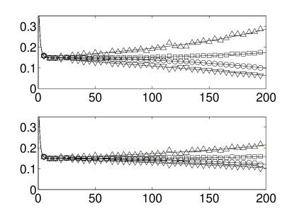
Figure 1: LVQ1 in the presence of concept drift. Solid lines correspond to the integration of ODE with initialization as in Eq. (10). Cluster variances are $v_{+}\!=\!v_{-}\!=\!0.4$ and $\lambda=1$ in the density (3). Upper graphs correspond to LVQ1 without weight decay, lower graphs display results for $\gamma=0.05$ in (12). In addition, Monte Carlo results for $N=100$ are shown: class-wise errors $\epsilon^{\pm}(\alpha)$ are displayed as upward (downward) triangles, respectively; squares mark the reference error $\epsilon_{ref}(\alpha)$ (14); circles correspond to $\epsilon_{track}(\alpha)$ (15). Left panel: drift with linearly increasing $p_{+}(\alpha)$ given by $\alpha_{o}\!=\!20$, $\alpha_{end}\!=\!200$, $p_{max}\!=\!0.8$ in (16). Right panel: sudden change of class weights according to to Eq. (17) with $\alpha_{o}=100$ and $p_{max}=0.75$. Only the $\alpha$-range close to $\alpha_{o}$ is shown.

Here, we will focus on non-stationary prior weights $p_{+}(\alpha)=1-p_{-}(\alpha)$ for the generation of example data. In this case, a varying fraction of examples represents each of the classes in the stream of training data. Non-stationary class bias complicates the training significantly and can lead to inferior performance in practical situations [25].

(A) Drift in the training data only

Here we assume that the target classification is defined by a fixed reference density of data. As a simple example we consider equal priors $p_{+}=p_{-}=1/2$ in a symmetric reference density (3) with $v_{+}=v_{-}$. On the contrary, the characterstics of the observed training data is assumed to be time-dependent. In particular, we study the effect of time-dependent $p_{\sigma}(\alpha)$ and weight decay.

Given the order parameters of the learning systems in the course of training, the corresponding reference generalization error

$$\epsilon_{ref}(\alpha)=\left(\epsilon^{+}+\epsilon^{-}\right)/2$$ (14)

is obtained by setting $p_{+}=p_{-}=1/2$ in Eq. (11), but inserting $R_{S\tau}(\alpha)$ and $Q_{ST}(\alpha)$ as obtained from the integration of the ODE (9) or (13) with time dependent $p_{+}(\alpha)=1-p_{-}(\alpha)$ in the training data.

(B) Drift in training and test data

In the second interpretation we assume that the time-dependence of $p_{\sigma}(\alpha)$ affects both the training and test data in the same way. Hence, the change of the statistical properties of the data is inevitably accompanied by a modification of the target classification: For instance, the Bayes optimal classifier and its best linear approximation will depend explicitly on the current priors $p_{\sigma}(\alpha)$ [12].

The learning system is supposed to track the drifting concept and we denote the corresponding generalization error, cf. Eq. (11), by

$$\epsilon_{track}=p_{+}(\alpha)\epsilon^{+}+p_{-}(\alpha)\epsilon^{-}.$$ (15)

In terms of modelling the training dynamics, both scenarios, (A) and (B), require the same straightforward modification of the ODE system: the explicit introduction of $\alpha$-dependent quantities $p_{\sigma}(\alpha)$ in Eq. (9). However, the obtained temporal evolution translates into the reference error $\epsilon_{ref}(\alpha)$ for the case of drift in the training data (A), and into $\epsilon_{track}(\alpha)$ in interpretation (B).

3 Results and Discussion

Here we present and discuss first results obtained by integrating the systems of ODE for LVQ1 with and without weight decay under different time-dependent drifts. For comparison, averaged learning curves as obtained by means of Monte Carlo simulations are also shown. All results are for constant learning rate $\eta=1$ and the LVQ systems were initilized according to Eq. (10).

We study three example scenarios for the time-dependence $p_{+}(\alpha)=1\!-p_{-}(\alpha)$:

Linear increase of the bias
We consider a time-dependent bias of the form $p_{+}(\alpha)=1/2\mbox{~{}for~{}~{}}\alpha<\alpha_{o}$ and

$$p_{+}(\alpha)=1/2+\frac{(p_{max}\!-\!1/2)\,(\alpha-\alpha_{o})}{(\alpha_{end}-\alpha_{o})}\mbox{~{}for~{}~{}}\alpha\geq\alpha_{o}.$$ (16)

where the maximum class weight $p_{+}=p_{max}$ is reached at learning time $\alpha_{end}$. Fig. 1 (left panel) shows the learning curves as obtained by numerical integration of the ODE together with Monte Carlo simulation results for $(N=100)$-dimensional inputs and prototype vectors. As an example we set the parameters to $\alpha_{o}=25,p_{max}=0.8,\alpha_{end}=200$. The learning curves are displayed for LVQ1 without weight decay (upper) and with $\gamma=0.05$ (lower panel). Simulations show excellent agreement with the ODE results.

The system adapts to the increasing imbalance of the training data, as reflected by a decrease (increase) of the class-wise error for the over-represented (under-represented) class, respectively. The weighted over-all error $\epsilon_{track}$ also decreases, i.e. the presence of class bias facilitates smaller total generalization error, see [12]. The performance with respect to unbiased reference data detoriorates slightly, i.e. $\epsilon_{g}$ grows with increasing class bias as the training data represents the target less faithfully.

The influence of the class bias and its time-dependence is reduced significantly in the presence of weight decay with $\gamma>0$, cf. Fig. 1 (lower panel). Weight decay restricts the norm of the prototypes, i.e. the possible offset of the decision boundary from the origin. Consequently, the tracking error slightly increases, while $\epsilon_{ref}$ with respect to the reference density is decreased compared to the setting without weight decay, respectively.

Sudden change of the class bias 
Here we consider an instantaneous switch from high bias $p_{max}>1/2$ to low bias:

$$p_{+}(\alpha)=p_{max}\mbox{~{}for~{}~{}}\alpha<\alpha_{o}\mbox{~{}~{}and~{}~{}}p_{+}(\alpha)=1-p_{max}\mbox{~{}for~{}~{}}\alpha\geq\alpha_{o}.$$ (17)

We consider $p_{max}=0.75$ as an example, the corresponding results from the integration of ODE and Monte Carlo simulations are shown in Fig. 1 (right panel) for training without weight decay (upper) and for $\gamma=0$ (lower panel).

  

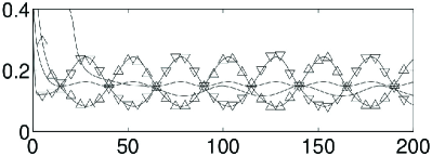
Figure 2: LVQ1 in the presence of oscillating class weights according to Eq. (18) with parameters $T=50$ and $p_{max}=0.8$, without weight decay $\gamma=0$ (left) and for $\gamma=0.05$ (right). For clarity, Monte Carlo results are only shown for the class-conditional errors $\epsilon^{+}$ (upward) and $\epsilon^{-}$ (downward triangles). All other settings as in Fig.  1.

We observe similar effects as for the slow, linear time-dependence: The system reacts rapidly with respect to the class-wise errors and the tracking error $\epsilon_{track}$ maintains a relatively low value. Also, the reference error $\epsilon_{ref}$ displays robustness with respect to the sudden change of $p_{+}$. Weight decay, as can be seen in the lower right panel of Fig.1 reduces the over-all sensitivity to the bias and its change: Class-wise errors are more balanced and the weighted $\epsilon_{track}$ slightly increases compared to the setting with $\gamma=0$.

The weight decay does not seem to have a notable effect on the promptness of the system’s adaptation to the changing bias. While it significantly regularizes the system, the expected effect of forgetting previous information in favor of the most recent examples cannot be observed.

Periodic time dependence  
As a third scenario we consider an oscillatory modulation of the class weights in training:

$$p_{+}(\alpha)=1/2+(p_{max}-1/2)\,\cos\left[2\pi\,{\alpha}\big{/}{T}\right]$$ (18)

with periodicity $T$ on $\alpha$-scale and maximum amplitude $p_{max}<1$.

Example results are shown in Fig. 2 for $T=50$ and $p_{max}=0.8$. Monte Carlo results for $N=100$ are only displayed for the class-wise errors show excellent agreement with the numerical integration of the ODE for training without weight decay (left panel) and for $\gamma=0.05$ (right panel). The observations confirm our findings for slow and sudden changes of $p_{+}$: In the main, weight decay limits the reaction of the system to the presence of a bias and its time-dependence.

4 Summary and Outlook

In summary, we have presented a mathematical framework in which to study the influence of concept drift on prototype-based classifiers systematically. In all specific drift scenarios considered here, we observe that simple LVQ1 can track the time-varying class bias to a non-trivial extent: In the interpretation of the results in terms of real drift, the class-conditional performance and the tracking error $\epsilon_{track}(\alpha)$ clearly reflect the time-dependence of the prior weights.

In general, the reference error $\epsilon_{ref}(\alpha)$ with respect to class-balanced test data, displays only little deterioration due to the drift in the training data.

The main effect of introducing weight decay is a reduced overall sensitivity to bias in the training data: Figs. 1-3 display a decreased difference between the class-wise errors $\epsilon^{+}$ and $\epsilon^{-}$ for $\gamma>0$. Naïvely, one might have expected an improved tracking of the drift due to the imposed forgetting, resulting in, for instance, a more rapid reaction to the sudden change of bias in Eq.  (17). However, such an improvement cannot be confirmed. Our findings are in contrast to a recent study [8], in which we observe increased performance by weight decay for a different drift scenario, i.e. the randomized displacement of cluster centers.

The precise influence of weight decay clearly depends on the geometry and relative position of the clusters. Its dominant effect, however, is the regularization of the LVQ system by reducing the norms $Q_{++}$ and $Q_{--}$ of the prototype vectors. Consequently, the NPC classifier is less flexible to reflect class bias which would require significant offset of the prototypes and decision boundary from the origin. This mildens the influence of the bias (and its time-dependence) and results in a more robust behavior of the employed error measures.

Alternative mechanisms of forgetting should be considered which do not limit the flexibility of the LVQ classifier, yet facilitate forgetting of older information. As one example strategy we intend to investigate the accumulation of additive noise in the training process. We will also explore the parameter space of the model density and in greater depth and study the influence of the learning rate systematically.

4.0.1 Acknowledgement

The authors would like to thank A. Ghosh, A. Witoelar and G.-J. de Vries for useful discussions of earlier projects on LVQ training in stationary environments.

References

- [1] I. Zliobaite, M. Pechenizkiy, and J. Gama. An overview of concept drift applications. In Big Data Analysis: New Algorithms for a New Society. Springer, 2016.
- [2] T. Hastie, R. Tibshirani, and J. Friedman. The Elements of Statistical Learning: Data Mining, Inference, and Prediction. Springer, 2001.
- [3] K. Amunts et al., editor. Brain-Inspired Computing, Second International Workshop BrainComp 2015, volume 10087 of LNCS. Springer, 2014.
- [4] V. Losing, B. Hammer, and H. Wersing. Incremental on-line learning: A review and of state of the art algorithms. Neurocomputing, 275:1261–1274, 2017.
- [5] G. Ditzler, M. Roveri, C. Alippi, and R. Polikar. Learning in nonstationary environment: a survey. Comput. Intell. Mag., 10(4):12–25, 2015.
- [6] J. Joshi and P. Kulkarni. Incremental learning: areas and methods - a survey. Int. J. Data Mining Knowl. Manag. Process., 2(5):43–51, 2012.
- [7] R. Ade and P. Desmukh. Methods for incremental learning - a survey. Int. J. Data Mining Knowl. Manag. Process., 3(4):119–125, 2013.
- [8] M. Straat, F. Abadi, C. Göpfert, B. Hammer, and M. Biehl. Statistical mechanics of on-line learning under concept drift. Entropy, 20(10), 2018. Art. No. 775.
- [9] T. Kohonen. Self-Organizing Maps, volume 30 of Springer Series in Information Sciences. Springer, 2001. (2nd edition).
- [10] D. Nova and P.A. Estevez. A review of Learning Vector Quantization classifiers. Neural Comput. Appl., 25(3-4):511–524, 2014.
- [11] M. Biehl, B. Hammer, and T. Villmann. Prototype-based models in machine learning. Wiley Interdisciplinary Reviews: Cognitive Science, 7(2):92–111, 2016.
- [12] M. Biehl, A. Ghosh, and B. Hammer. Dynamics and generalization ability of LVQ algorithms. J. Machine Learning Res., 8:323–360, 2007.
- [13] D. Saad, editor. On-line learning in neural networks. Cambridge Univ. Press, 1999.
- [14] A. Engel and C. van den Broeck. The Statistical Mechanics of Learning. Cambridge University Press, 2001.
- [15] T.L.H. Watkin, A. Rau, and M. Biehl. The statistical mechanics of learning a rule. Rev. Mod. Phys., 65(2):499–556, 1993.
- [16] M. Biehl, A. Freking, and G. Reents. Dynamics of on-line competitive learning. Europhys. Lett., 38:73–78, 1997.
- [17] N. Barkai, H.S. Seung, and H. Sompolinsky. Scaling laws in learning of classification tasks. Phys. Rev. Lett., 70(20):L97–L103, 1993.
- [18] C. Marangi, M. Biehl, and S. A. Solla. Supervised learning from clustered input examples. Europhys.Lett., 30:117–122, 1995.
- [19] M. Biehl and H. Schwarze. Learning drifting concepts with neural networks. J. Phys. A: Math. and Gen., 26:2651–2665, 1993.
- [20] R. Vicente and N. Caticha. Statistical mechanics of on-line learning of drifting concepts: A variational approach. Machine Learning, 32(2):179–201, 1998.
- [21] G. Reents and R. Urbanczik. Self-averaging and on-line learning. Phys. Rev. Lett., 80(24):5445–5448, 1998.
- [22] M. Mezard, J.P. Nadal, and G. Toulouse. Solvable models of working memories. J. de Phys. (Paris), 47(9):1457–1462, 1986.
- [23] J.L. van Hemmen, G. Keller, and R. Kühn. Forgetful memories. Europhysics Letters, 5(7):663–668, 1987.
- [24] D. Saad and S.A. Solla. Learning with noise and regularizers in multilayer neural networks. In Neural Inf. Proc. Syst. (NIPS 9), pages 260–66. MIT Press, 1997.
- [25] Shuo Wang, Leandro L. Minku, and Xin Yao. A systematic study of online class imbalance learning with concept drift. CoRR, abs/1703.06683, 2017.