Vegetation pattern formation in a sinuous free-scale landscape

Abstract

The original Hardenberg’s model of biomass patterns in arid and semi-arid regions is revisited to extend it to more general -non flat- regions. It is proposed a technique to study these more generalized (non-flat) regions using both a conservation criterion and a explicit spatial dependant function $\nu(x)$. In this paper a study of dynamical stability around sistem’s fixed points made. Under the idea of predictibility via air images a fitted relationship among dynamical variables at stable fixed points is stablished. Also, is presented a discrete version of the model, in the form of Cellular Automata thechniques, that allows to neglect the spatial scale and reproduces realistic stable spatial patterns.

Keywords: Ecosystems, Biomass patterns, Reaction-Diffusion, Dessertic regions

1 Introduction

The structure and dynamics of ecosystems are extremely complex. The interactions among the multiple species and its interactions with their landscape, climate conditions and human behaviour are quite complex. There exists a lot of ways in which these interactions can be present, in particular in the animal-vegetation interactions case, where they can change the behavior and population of both vegetation and animal species. In recent ecology studies [Boyer et al., 2006] has been shown that the inhomegeneities in food resources modifies the foraging walk dynamics of herbivore species. This inhomegeneities can be modeled in a spatial sense or in terms of their importance or size as food resources.
Not only the walking dynamics but the social behavior of animal population could be modified, as the Ramos-Fernández et. al. [Ramos-Fernández et al., 2006] model suggests. The subgroups formation in hervibore mammals create a social network which structure depends on the conjugation of animal’s memory and the food patches size distribution. Furthermore, animal and vegetation species can be thinked as “ecosystem’s engineers”, i. e., key species that modulate the introducction, permanence or extintion of another ones in the ecosystem [Gilad et al., 2004].

In the case of ground vegetation, these interactions could be the responsibles of the wide variety of propagation, stablishment and survive strategies. For example, vegetation propagation can be done via seed dispersion, by hervibores or by wind, and by asexual reproduction, in which a new individual is conected to the parental plant. The latter is important in low humidity regions because the conection with the parental plant provides the new one a certain independence of landscape characteristics, such as surface watter or soil nutrient availability. Also, recent work of Thompson [Thompson et al., 2008] shows that seed dispersal mechanism changes the spatial configuration of vegetation, destabilizing the regular patterns observed in diffusion-based models. In the other hand, propagation via seeds gives the vegetation another way to survive, as the seeds can be lattent, in some cases, for long time periods between seed dispersal and germination, and, furthermore, the seeds can survive low watter or fire regimes. In the latter case, there are seeds that survives high temperatures regimes, around $90^{\circ}C$, as observed in Bombax tomentosum, Bowdicha major, Brosimum gaudichaudii and other species. Indeed, another seed species seem to be favoured by this situation, for example M. pubescens and B. major [Garca-Núñez and Azócar, 2004].

As above, interactions between vegetation and soil features are diverse. As an example, it is observed that the flower and fruit generation in some species are sinchronized with dry season in savhannas, wich is an evidence of deep watter resources available for some species. Also, soil nutrients distribution could be an important feature in the species spatial configuration, as in savhannas where is observed a grassland continous matrix ocasionally interrupted by low density tree patches.

Also, vegetation dynamics can modulate their landscape and the pressence or absence of animal populations. Vegetation is traditionaly used for soil recovering, as it prevents erosion via its roots, for soil structure improvement, as it provides physical support and organic matter addition, and acelerates nutrient fixation process.

Another interesting feature of vegetation dynamics is the pattern formation process which is supposed to be the result of cooperation and competition mechanisms between vegetation patches in a limited resources landscape [von Hardenberg et al., 2001], relationships between bacteria and vegetation species [Gilad et al., 2004] and stochastic phenomena [Shnerb et al., 2003]. The Figure below, shows some vegetation patterns observed in arid and semiarid lands.

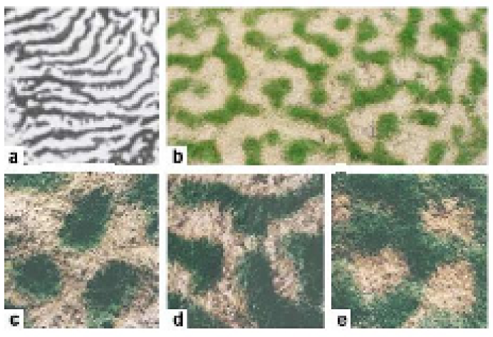
Figure 1: Original image taken of Hardenberg’s paper [von Hardenberg et al., 2001]. The scales in the size of biomass patterns are quite different: from centimeters (for patterns $c$, $d$ and $e$) to tens of meters (patterns $a$ and $b$)

.

As sketched above, these interactions, and several another, are extremely complicated to model, but it is important to account them in the search for more complete and accurate descriptions of ecosystems dynamics. It is necessary to consider both animal species in mutual interactions and the vegetal species vinculated with the animal behavior. Mineral resources, weather, humedity, chemical and physical properties of soil and different type of relations between species are topics of importance in this theme. However, a model that consider all the interactions mentioned above will be quite complicated.

On the other hand, there exists simplified models and reports that enables the comprehension of some interesting and important aspects of this system. These models are developed using different techniques, such as Partial Differential Equations (PDE), Reaction-Diffusion Systems (RDS), Cellular Automata (CA), etc. For example, the work cited at Solé’s book [Solé and Manrubia,] consists of a simple CA model to describe the observed behavior in some american and japanesse rainforest regions, called Shigamare effect. These regions presents a kind of propagating “wave front” of dead trees over the entire forest. In Solé’s model, each cell of the CA represents, via its value, a tree of some size (or age). The temporal evolution of the tree size depends on the average size of its neighborhood and on the wind direction. These assumptions are the responsibles of the dynamic patterns obtained with this model shown in Figure 2.

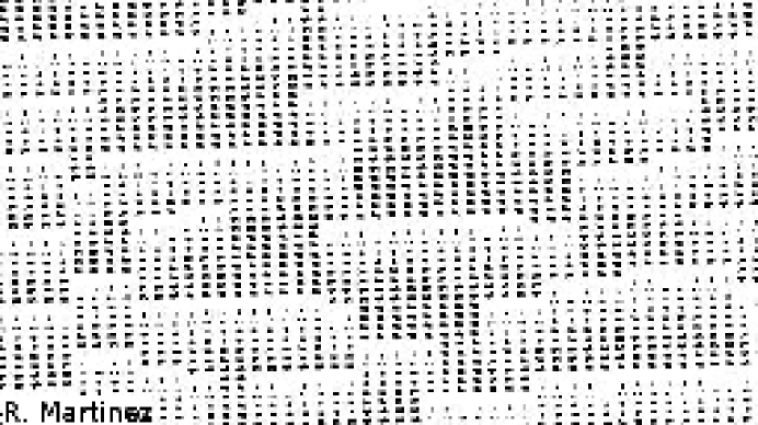
Figure 2: Shigamare dynamic patterns of propagating wave front. Dead trees are represented by darkest cells.

Another approach to vegetation dynamics was made by Manor and Shnerb for the vegetation patterns observed in arid and semi-arid regions near Jerusalem and Nigeria [Manor and Shnerb, 2008]. This model consists on two diferential equations, one for biomass and another for soil water density which are modeled as discrete local variables as values in a finite lattice of lenght $L$. They consider a positive feedback mechanism related with two process of vegetation mortality: below a threshold size the new vegetation shrubs wont survive and natural death. Both mechanisms are stochastic and obey two kinds of probabilities which depends on the distance between shrubs and the threshold size. The results of this model are presented in terms of stable vegetation patterns and Lévy-like patches size distributions as shown in Figure 3.

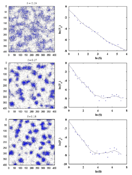
Figure 3: Spatial vegetation patterns and patches size distributions obtained vía Shnerb’s model. Note that in the second and third distributions the Lévy-like regime is lost.

.

The aim of this work is, in one hand, to make a detailed analysis of Hardenberg’s model related with its fixed points, stability around them and to study statistical distributions of biomass densities. The other part of this study is related with the possibility that, under random initial conditions in a uniform grid, this model can generate the biomass patterns in a non-flat region.

In section 2 the stability analysis of the Hardenberg’s model is done, showing that, close to the non obvious fixed point, the system is asymptotically stable and the biomass density tends to a value that depends on the $p$ parameter. Also, here is proposed a discrete version of the original model that conduces to the neglecting posibility of the spatial scale and two ways to generalize the vegetation patterns in a non-flat region. Section $3$ is devoted to the results obtained in terms of vegetation patterns formation and the biomass density dristributions. Finally, a discussion over the results is in Section 4.

2 Hardenberg’s model

The original model of Hardenberg [von Hardenberg et al., 2001] consists of a pair of dynamical equations that involves terms related with diffusion for both green biomass (plants) density $n$ and soil humidity $w$. The coupled equations are

$$\frac{\partial n}{\partial t}=\frac{\gamma w}{1+\sigma w}n-n^{2}-\mu n+\nabla^{2}n$$ (1)

and

$$\frac{\partial w}{\partial t}=p-(1-\rho n)w-nw^{2}+\delta\nabla^{2}(w-\alpha n)+v\frac{\partial(w-\beta n)}{\partial x}$$ (2)

The first term in Eq. (LABEL:h1) accounts for the biomass growth rate with the present local biomass and a coefficient that accounts for a limited influence of the pressence of humidity. The second term is vinculated with finitude of resources, as in logistic model of populations growth [Strogatz, 1994]. Quantity $-\mu n$ represents dead of vegetation, due both to herbivores and natural mortality. In second equation, $p$ is a source term for the humidity, as an annual rain average. Second and third terms are related to watter loss due evaporation, which is reduced in the presence of vegetation by the factor $(1-\rho n)$, and due to watter uptake by the vegetation’s roots. In both equations, the spatial terms, $\nabla^{2}n$ and $\delta\nabla^{2}(w-\alpha n)$, models the diffusion of biomass and humidity in space, with the latter reduced by the prescence of biomass. In the last term in Eq. (2.2), $v$ is the watter runoff velocity towards direction $x$, where a hill slope is assumed, and the partial derivate models the humidity diffusion in this direction.

With these assumptions, Hardenberg’s model show a good aproximation to real vegetation patterns (Figure 1) as can be seen in Figure 4.

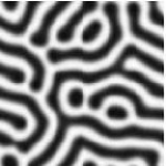
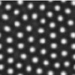
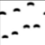
Figure 4: Vegetation patterns resulting from Hardenberg’s model. Note the linear behaviour of banded patterns. Reprinted figures with permission from: J. von Hardenberg, E. Meron, M. Shachak and Y. Zarmi. Physical Review Letters 87, 198101-1, 2001. Copyright(2001) by the American Physical Society. http://prl.aps.org/abstract/PRL/v87/i19/e198101

2.1 Stability analysis

In order to know the possible correlations between local biomass density, humidity and the control parameter $p$ -that defines the model dynamic behavior- in this section we made a linear stability analysis [Strogatz, 1994], which enable us to find all the system’s fixed points in terms of $p$.

If we define

$$F_{n}(n,w)=\frac{\gamma w}{1+\sigma w}n-n^{2}-\mu n$$

and

$$F_{w}(n,w)=p-(1-\rho n)w-nw^{2},$$

fixed points $(n^{\star},w^{\star})$ of the system

$$\frac{\partial n}{\partial t}=F_{n}(n,w) \frac{\partial w}{\partial t}=F_{w}(n,w)$$ ;

are obtained for each value of $p$ solving $F_{n}(n^{\star},w^{\star})=F_{w}(n^{\star},w^{\star})=0$. So, with the aim of determining the stability of Hardenberg’s model, we evaluate the aproximate numerical values of the fixed points for a series of values of $p$ parameter, some of them shown in Table 1.

$p$	0.20	0.30	0.40	0.50	0.60	0.70	0.80	0.90
$n^{\star}$	0.05654	0.17379	0.26110	0.32059	0.36225	0.39308	0.41704	0.43639
$w^{\star}$	0.21566	0.37306	0.53477	0.67871	0.80276	0.91093	1.00703	1.09387

Table 1: Fixed Points obtained numerically for some values of $p$. The other parameters are  $\delta=100,\alpha=3,\beta=3,\sigma=1.6,\gamma=1.6,\mu=0.2,\rho=1.5$ in all the calculations.

In making the linear stability analysis we define $u_{n}=n-n^{\star}$ and $u_{w}=w-w^{\star}$, whose numeric values are small, and construct the jacobian matrix associated with the dynamical system. Then, the original model in a small region around fixed points can be wroten as:

$$\left(\begin{array}[]{l}\frac{\partial u_{n}}{\partial t}\\ \\ \frac{\partial u_{w}}{\partial t}\end{array}\right)=\left(\begin{array}[]{ll}\left.\frac{\partial F_{n}}{\partial n}\right|_{P^{\star}}&\left.\frac{\partial F_{n}}{\partial w}\right|_{P^{\star}}\\ &\\ \left.\frac{\partial F_{w}}{\partial n}\right|_{P^{\star}}&\left.\frac{\partial F_{w}}{\partial w}\right|_{P^{\star}}\end{array}\right)\left(\begin{array}[]{l}u_{n}\\ \\ u_{w}\end{array}\right).$$

It is found that all eigenvalues of the Jacobian matrix are negative and, then, all fixed points are attractor points: the model is stable near of these points.

In correspondence, neglecting the explicit spatial terms in the original equations (1) and (2), a rasoneable set of initial conditions is selected with the aim of verify that the $[0,1]\times[0,1]$ region of phase space is contained in an attraction basin [Strogatz, 1994] and to evaluate the dynamical evolution of the variables. Some fixed points are presented in Figure 5 with small white circles and the particular ones, associated with each $p$ value, as an out-of-axis big black dot.

Figure 5: All the initial conditions for $n$ and $w$ in the phase space for $p=0.1,0.2,\ldots,0.6$ leads the system toward its fixed points. Square symbols represents initial conditions. Filled black dots are the fixed points for a particular $p$ and white circles shows a sequence of fixed points for $p=0.1,\ldots,0.8$. For each $p$ value the obvious fixed point $(0,p)$ is on the left of image, except in a) where $n^{\star}<0$. All the images above were performed for 300,000 discrete time steps. Arrows in a) show the flow direction.

It is clear, from Figure 5 a), that very small values in the $p$ parameter has no sense in the dynamics of $n$ and $w$. The fixed poin for $p=0.1$, for example, corresponds to a negative value of the biomass density $n$, and appears at the left of the $(0,p)$ fixed point.

The shown sequence of fixed points (small white circles in Figure 5) appears to be a functional relationship between the $w$ and $n$ variables that could be used to determine humidity density from biomass density values. In Figure 6 is shown an exponential curve fitted over the fixed points which represents the functional relationship between biomass and humidity fixed points

.

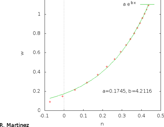
Figure 6: Fitted fixed points in phase space of Hardenberg’s model for diferent $p$ values.

2.2 Discretization

Note that the nonlinear character of equations (1) and (2) implies the numeric solution of the first order temporal part by means oIn a similar grid than Figure 11 using the smoothing function $\nu(x)$ in Eq. (8). The pictures above were rotated $180^{\circ}$ to show the correspondence with those in Figure 12f an appropiate numeric approximation, using some general numeric algorithm such as Euler or Runge-Kutta methods.

In the spatial case, the discretización via finite differences of the diffusion (laplacian) operator implies that the neighboring cells to each one modifies the local state of last. If the grid has a size $h$, or the cells $h^{2}$, in the lattice then, for a continuous $C^{2}$ class function, must be true:

$$\nabla^{2}u(x,y,t) \simeq \frac{1}{h^{2}}[u(x+h,y,t)+u(x-h,y,t)+$$

$$+u(x,y+h,t)+u(x,y-h,t)-4u(x,y,t)].$$ (3)

In order to observe how the model’s dynamics can develop the desired spatial patterns, it is important that these patterns can be obtained from a local random initial state. However, in doing so, the function $u$ does not longer belong to $C^{2}$ class functions, and the algorithm stability disappears. So that, in order to stablish random values at $t=0$, we redefine the discrete Laplace’s operator as:

$$\nabla^{2}u_{i,j}^{t}=u^{t}_{i,j+1}+u^{t}_{i,j-1}+u^{t}_{i+1,j}+u^{t}_{i-1,j}-4u^{t}_{i,j},$$ (4)

where the symbol $u_{i,j}^{t}$ represents the value, at time $t$, of cell $(i,j)$ of the generic variable $u$. This approximation is justified numerically, as sketched above, and also because the scales of the biomass patterns are quite different (see Figure 1): by defining $h=1$, the scale in the model is arbitrary and the discrete laplacian measures the influence of neighbor cells on the actual one. This idea is similar to those used in CA techniques in modeling several systems dynamics An important question about this redefinition of the discrete laplacian term is if the assumptions made avobe affect the performance of the model’s emergent spatial patterns. The answer is in the negative sense, as can be seen in Figures 8, 9 and 10.

Thus, Eq. (1) and (2) can be rewriten in their discrete version both temporal, using Euler’s method,  and spatial as:

$$n^{t+1}_{i,j}=\left(\frac{\gamma w^{t}_{i,j}}{1+\sigma w^{t}_{i,j}}n^{t}_{i,j}-{n^{t}_{i,j}}^{2}-\mu n^{t}_{i,j}+\nabla^{2}n^{t}\right)\Delta t+n^{t}_{i,j}$$ (5)

$$w^{t+1}_{i,j}=\left(p-(1-\rho n)w^{t}_{i,j}-n{w^{t}_{i,j}}^{2}+\delta\nabla^{2}(w^{t}-\alpha n^{t})+v\frac{\partial(w^{t}-\beta n^{t})}{\partial x}\right)\Delta t+w^{t}_{i,j}.$$

where

$$\nabla^{2}n^{t}=n^{t}_{i,j+1}+n^{t}_{i,j-1}+n^{t}_{i+1,j}+n^{t}_{i-1,j}-4n^{t}_{i,j}$$

,

$$\nabla^{2}(w^{t}-\alpha n^{t})=w^{t}_{i,j+1}+w^{t}_{i,j-1}+w^{t}_{i+1,j}+w^{t}_{i-1,j}-4w^{t}_{i,j}-\alpha\nabla^{2}n^{t}$$ (6)

and

$$\frac{\partial(w^{t}-\beta n^{t})}{\partial x}=\frac{w^{t}_{i+1,j}+w^{t}_{i-1,j}-\beta(n^{t}_{i+1,j}+n^{t}_{i-1,j})}{2}$$ (7)

2.3 Non flat regions

In the search of a more complete model of arid and sem-arid ecosystems, a simplification of non flat regions, where there is no constant slope, is introduced because vegetation patterns disappear in Hardenberg’s model when two different slope areas are used as the region where vegetation dynamics takes place.

As a first attempt, a pair of joined plane regions, one of them with no null slope, are considered, opposite of what was done in Hardenberg’s model where diferent slope regions are treated separately, as can be seen in Figure 4. This assumption is justified by field reports as in [Gessler et al., 2000], so that any small or more or less regular region can be mapped by means of this two-region model. It is necessary to stablish adecuate boundary conditions in order to avoid the introduction of unphysical elements, and must reflect the natural dynamics of watter diffusion, as limitting resource.

First of all, as a lattice of size $L\times L$ is used, the joint point within both regions is taken at a position $L/2$ over direction $x$, so the parameter $\nu$ is non zero for $x\leq L/2$ and equal to zero after this limit, for all the cells in the grid. In the extreme left, where hill begins, and in the extreme right, where the flat region ends, null and null flux border conditions are considered respectively, both for biomass and watter densities. In the direction $y$, where no slope effects are considered, periodicall border conditions are taken.

In the joint region the border conditions can not be arbitrarily selected. The watter runnoff ends in a zero slope region increasing the humidity available for biomass growth there and, then, it begins to spread. Thus, in order to take account for this humidity increase, the average of watter runoff term in its discret form (7), taken over each cell of the sloping region, is added to the correspondent first cell of the grid with zero slope. This average takes the form:

$$<w_{x}>=\frac{v}{L}\sum_{j=1}^{\frac{L}{2}}[w_{k,i+1,j}-w_{k,i-1,j}-\alpha(n_{k,i+1,j}-n_{k,i-1,j})],$$

Whith this construction, several runs were performed in order to reproduce spatial veggetation patterns in both regions, and the results can be observed in Figure 12. The patterns shows certain similarity with those in real pictures and in the original results of Hardenberg’s model (Figures 1 and 4). Although these “hybrid” patterns are a good aproximation to the real ones, they are still quite regular and its shape can be improved using the idea of a non constant difussion coefficient, as was done in some texture synthesis works [Witkin and Kass, 1991, Sanderson et al., 2006], applied to water runoff term in Eq. (2).

In the last term of Eq. (2), the one associated with the partial derivative, the constant factor $\nu$ is now considered as an explicit spatial dependant function wich takes the form:

$$\nu(x)=\frac{1}{2}\nu\left[\tanh\left(\frac{20x}{l}-10\right)+1\right]$$ (8)

where parameter $\nu$ is taken as in Eq. (2) and $l$ is the number of unitary cells in lattice lenght $L$. As $\nu$ represents the watter runnoff velocity in a slope, this new function represents a region where slope is slightly increased from $0$ to a maximum value $\nu(x)=\nu$ as the position in the direction $x$ is increased. In doing so, it is clear that the joint conditions, explained above, are now unnecessary.

In this aproach, zero flux border conditions are considered for the left and right extremes over $x$ direction and periodical border conditions over direction $y$. The resulting patterns are shown in Figure 13, and can be observed a significant improvement in the similarity with real patterns (Figure 1).

3 Results

In order to know the possible correlations between local biomass density, humidity and the control parameter $p$ -that defines the model dynamic behavior- in this section vegetation density distributions for some fixed values of $p$ and the spatial patterns obtained in a non flat region with both aproaches explained in Section 2.3 are shown.

Consistence in a possible predictibility criterion implies that the temporal evolution of the variables leads them toward its fixed point values. Statistical distribution of biomass density, evaluated on all cells of the lattice for some $p$ values, are shown in Figure 7 and its observed that its behavior depends on the $p$ parameter value.

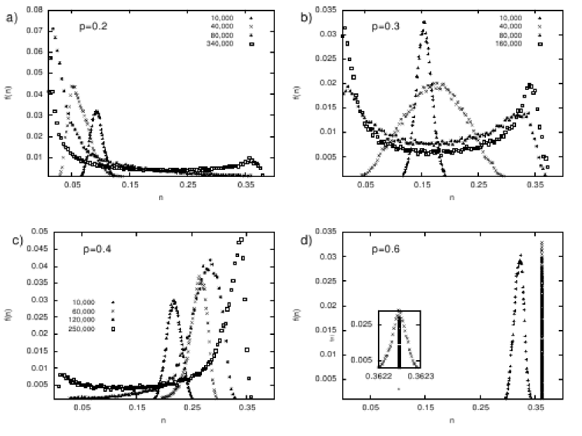
Figure 7: Evolution and stable statistical distributions of biomass density for some characteristic values of $p$. The fixed points for each $p$ value are: a) $n^{\star}=$ 0.05654; b) $n^{\star}=$0.17379; c) $n^{\star}=$0.26110 and d) $n^{\star}=$0.36225. Observe that biomass density distributions begins around fixed points values in all cases (marked with $+$), and that there exists a stable characteristic value for biomass density above $n=0.35$.

The stable statistical distribution curve of biomass density (with small square points in all images of Figure 7) changes, when $p$ does, from predominant high values for small $n$ (see Figure 7a) with a small protuberance near of $n\simeq 0.36$ (for $p=0.2)$, in passing by predominant small and high $n\simeq 0.36$ values of density (Figure 7b), toward a delta distribution for high values of $p$ (Figures 7c and 7d). In all cases, statistical distributions begins at values near to its respective fixed point and, as can be seen in the inset in Figure 7d, only one tends to this value. In the other cases (7a, 7b and 7c) the distribution moves away from the fixed point.

Figures 8, 9, 10 and 11 shows the stable emergent patterns of biomass spatial distribution. This patterns are in accordance with the real ones (Figure 1), and with those obtained by Hardenberg (Figure 4), which shows that a discrete version like that proposed in Section 2.2, where the evolution local of the variable $n$ depends on its neighbor values, is a good aproximation in order to qualitatively represent vegetation pattern formation process. In fact, models with evolution rules based in neighbor cell values, such as the CA models [Smith, 1994] and the above mentioned model of Shnerb [Manor and Shnerb, 2008], has shown acceptable results in modeling various dynamical systems [Solé and Manrubia,, Iwasa et al., 1991, Bascompté and Solé, 2005].

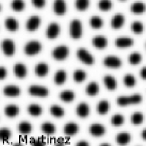
Figure 8: Hardenberg’s patterns of biomass: spots for $p=0.2$. Here the cells with very low values if density dominates the space.

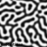
Figure 9: Evolution of biomass patterns toward a labyrinth for  $p\text{}=0.3$, the sites of low density are spacially distributed in analog to high density cells. This fact corresponds to a pair of stable maximum values in density distribution (see Fig. 7 b).

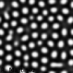
Figure 10: Evolution of Hardenberg’s biomass: holes for $p=0.4$, where high values of density dominates over low density regions.

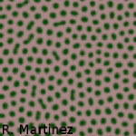
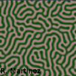
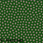
Figure 11: Patterns obtained from a $512\times 512$ grid with $\nu=0$.

Vegetation patterns obtained vía “joint” conditions and the smoothing function $\nu(x)$ are presented in Figures 12 and 13, respectively. Observe that in mixed patterns in the former (Figure 12) the association between banded patterns and those observed inThis null slope regions is near to the middle of the lattice, and, in both figures, this association is made via an unfinished banded pattern merged with those in zero slope region. Note that, while those presented in Figure 12 are in a certain way “regular” and de band is almost straight, patterns in Figure 13 are closer to real vegetation patterns.

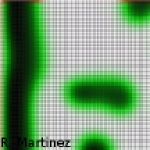
Figure 12: Left to right, p=0.2, 0.3, 0.4, same values of $p$ that in figures 8, 9 y 10. The patterns are combination of patterns: patterns of inclined surface (left in all grids)  joined with patterns of horizontal plane (right side on all grids).

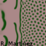
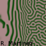
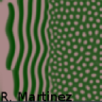
Figure 13: In a similar grid than Figure 11 using the smoothing function $\nu(x)$ in Eq. (8). The pictures above were rotated $180^{\circ}$ to show the correspondence with those in Figure 12

4 Discussion

The behaviour of biomass density patterns and the associated statistical distribution must be sufficient as criterion to determine biomass density from images and, eventually, they could be used in determination of zones in dessertification risk. Very small values of $n$ must correspond to null plants regions as can viewed from Figure 7a. Surprisingly, although the dynamical behaviour tends to the fixed points (phase portraits in Figure 5) biomass density distributions moves away from fixed point value, except for large $p$ values (Figure 7d). This is so because spatial patterns appear when a stationary stable state in absence of diffusion -in other words a fixed point- becomes unstable under diffusion, which is surprising because usually when a substance begins to spread, concentration gradients of it decreases in time, which leads to the disappearance of spatial configurations [Turing, 1952, Barrio, 2010]. In this cases, diffusion mechanism is responsible of pattern formation and of the behaviour observed in the statistical distibutions 7a, 7b and 7c.

Also, note that in Figure 7 no Lévy-like regime emerges in the statistical distributions of biomass density, although in Figure 7a, which corresponds to low $p$ values, a sort of broken Lévi-like regime, at high values of biomass density, is shown as was seen in the last image in Figure 3 for the patch size distribution of the model at [Manor and Shnerb, 2008].

Note that the pattern formation process continues even when the discretization criterion, and its consequent loss of scale, is applied to difussion term in Eqs. (1) and (2) as was explained in section 2.2. This simplification, chosed due to the need of obtain the spatial patterns from a randomized initial condition and due to the diferent scales of vegetation spatial patterns, shows a more realistic representation of spatial configurations presented as an emergent behaviour of vegetation in arid and semi-arid areas, as can be seen in Figure 1.

Furthermore, the “joint” conditions and spatial explicit dependance of watter runoff velocity $\nu$, in Eq. 2, proposed in Section 2.3, allows the creation of patterns that mix spatial shapes observed in nature (Figures 1 and 4), which can not be done with Hardenberg’s model alone, as the patterns disappear. Also, this construction brokes the linear behaviour of banded patterns obtained using Hardenberg’s model alone (Figure 4) making them closer to the real ones. Thus, the variable slope of the landscape could be another posible explanation to the irregularity of natural patterns (Figure 1) along with seed dispersal process, as was stablished in [Thompson et al., 2008].

Nevertheless, more general models can involve cooperation-competition events between different vegetal species doing modifications in the parameters $\rho$, associated with the external morphology of the plant in terms of shadow capacity, $\alpha$ with the absorption capacity -that diminishes the local diffusion of humidity- and $\beta$ that can be related with both the local absorption capacity and with a physical barrier that dumps the water flux. Also, the resulting patterns, and its associated vegetation density, could be used as food resource maps where foragers movement takes place, in a similar way as in [Boyer et al., 2006].

References

- [Barrio, 2010] Barrio, R. A. (2010). Aplicaciones del Modelo BVAM a Sistemas Complejos. Revista Digital Universitaria, 11(6).
- [Bascompté and Solé, 2005] Bascompté, J. and Solé, R. (2005). Margalef y el espacio o por qué los ecosistemas no bailan sobre la punta de una aguja. Ecosistemas, XIV(001).
- [Boyer et al., 2006] Boyer, D., Ramos-Fernández, G., Miramontes, O., Mateos, J. L., Cocho, G., Larralde, H., Ramos, H., and Rojas, J. F. (2006). Scale-free foraging by primates emerges from their interaction with a complex environment. Proceedings of the Royal Society B.
- [Garca-Núñez and Azócar, 2004] Garca-Núñez, C. and Azócar, A. (2004). Ecologa de la regeneración de árboles de la sabana. Ecotrópicos, 17(1-2).
- [Gessler et al., 2000] Gessler, P. E., Chadwick, O. A., Chamran, F., Althouse, L., and Holmes, K. (2000). Modeling Soil-Landscape and Ecosystem Properties Using Terrain Atributes. Soil Sci. Soc. Am. J., 64:2046–2056.
- [Gilad et al., 2004] Gilad, E., von Hardenberg, J., Provenzale, A., Shachack, M., and Meron, E. (2004). Ecosystem engineers: From pattern formation to habitat creation. Physical Review Letters, 93(9):098105.
- [Iwasa et al., 1991] Iwasa, Y., Sato, K., and Nakashima, S. (1991). Dynamic modeling of wave regeneration (Shigamare) in subalpine forests. J. Theor. Biol., 152.
- [Manor and Shnerb, 2008] Manor, A. and Shnerb, N. M. (2008). Facilitation, competition and vegetation patchiness: From scale free distribution to patterns. Journal of Theoretical Biology, 253:838–842.
- [Ramos-Fernández et al., 2006] Ramos-Fernández, G., Boyer, D., and Gómez, V. P. (2006). A complex social structure with fission-fusion properties can emerge from a simple foraging model. Behav. Ecol. Sociobiol., 60:536–549.
- [Sanderson et al., 2006] Sanderson, A. R., Kirby, R. M., Johnson, C. R., and Yang, L. (2006). Advanced Reaction-Diffusion Model for Texture Synthesis. Journal of Graphics, GPU and Game Tools, 11(3):47–71.
- [Shnerb et al., 2003] Shnerb, N. M., Sarah, P., Lavee, H., and Solomon, S. (2003). Reactive glass and vegetation patterns. Physical Review Letters, 90(3):038101.
- [Smith, 1994] Smith, M. A. (1994). Cellular Automata Methods in Mathematical Physics. PhD thesis, Massachusetts Institute of Technology.
- [Solé and Manrubia, ] Solé, R. V. and Manrubia, S. C. Orden y caos en sistemas complejos. Edicions UPC.
- [Strogatz, 1994] Strogatz, S. H. (1994). Nonlinear Dynamics and Chaos. Westview Press.
- [Thompson et al., 2008] Thompson, S., Katul, G., and McMahon, S. M. (2008). Role of biomass spread in vegetation pattern formation within arid ecosystems. Water Resources Research, 44.
- [Turing, 1952] Turing, A. M. (1952). A Chemical Basis of Morphogenesis. Phil. Trans. R. Soc. Lond., 37.
- [von Hardenberg et al., 2001] von Hardenberg, J., Meron, E., Shachack, M., and Zarmi, Y. (2001). Diversity of vegetation patterns and desertification. Physical Review Letters, 87(19).
- [Witkin and Kass, 1991] Witkin, A. and Kass, M. (1991). Reaction-Diffusion Textures. Computer Graphics, 25(4):299–308.