Bag of Tricks and A Strong Baseline for Deep Person Re-identification
Abstract
This paper explores a simple and efficient baseline for person re-identification (ReID). Person re-identification (ReID) with deep neural networks has made progress and achieved high performance in recent years. However, many state-of-the-arts methods design complex network structure and concatenate multi-branch features. In the literature, some effective training tricks are briefly appeared in several papers or source codes. This paper will collect and evaluate these effective training tricks in person ReID. By combining these tricks together, the model achieves 94.5% rank-1 and 85.9% mAP on Market1501 with only using global features. Our codes and models are available at https://github.com/michuanhaohao/reid-strong-baseline
1 Introduction
Person re-identification (ReID) with deep neural networks has made progress and achieved high performance in recent years. However, many state-of-the-arts methods design complex network structure and concatenate multi-branch features. In the literature, some effective training tricks or refinements are briefly appeared in several papers or source codes. This paper will collect and evaluate such effective training tricks in person ReID. With involved in all training tricks, ResNet50 reaches 94.5% rank-1 accuracy and 85.9% mAP on Market1501 [24]. It is worth mentioning that it achieves such surprising performance with global features of the model.
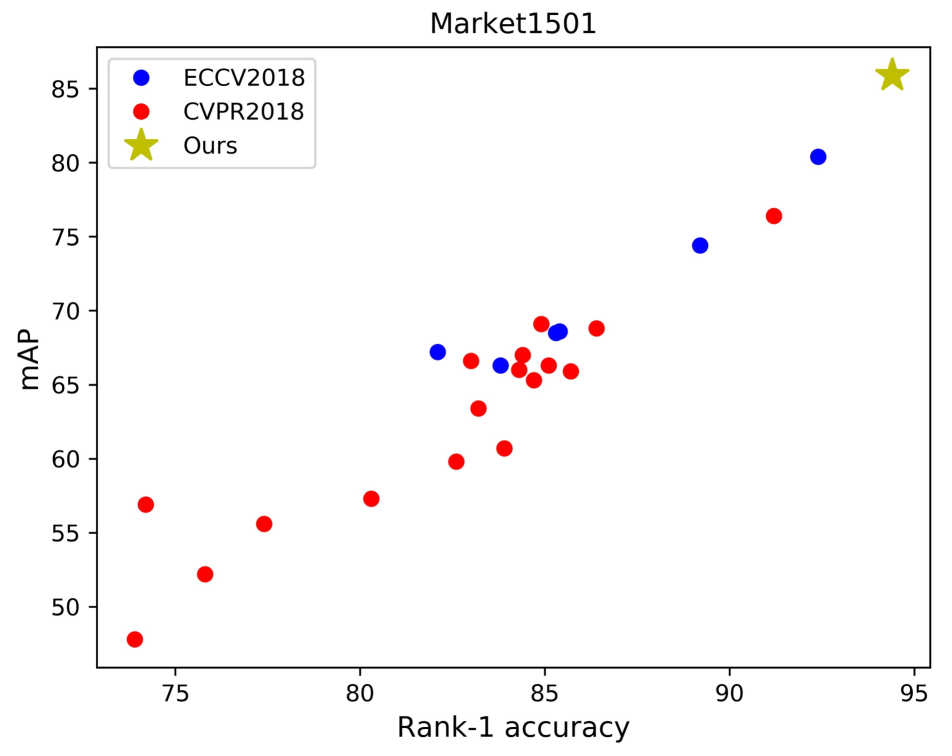
For comparison, we surveyed articles published at ECCV2018 and CVPR2018 of the past year. As shown in Fig. 1, most of previous works were expanded on poor baselines. On Market1501, only two baselines in 23 baselines surpassed 90% rank-1 accuracy. The rank-1 accuracies of four baselines even lower than 80%. On DukeMTMC-reID, all baselines did not surpass 80% rank-1 accuracy or 65% mAP. We think a strong baseline is very important to promote the development of research. Therefore, we modified the standard baseline with some training tricks to acquire a strong baseline. The code of our strong baseline has been open sourced.
In addition, we also found that some works were unfairly compared with other state-of-the-arts methods. Specifically, the improvements were mainly from training tricks rather than methods themselves. But the training tricks were understated in the paper so that readers ignored them. It would make the effectiveness of the method exaggerated. We suggest that reviewers need to take into account these tricks when commenting academic papers.
Apart from aforementioned reasons, another consideration is that the industry prefers to simple and effective models rather than concatenating lots of local features in the inference stage. In pursuit of high accuracy, researchers in the academic always combine several local features or utilize the semantic information from pose estimation or segmentation models. Such methods bring too much extra consumption. Large features also greatly reduce the speed of retrieval process. Thus, we hope to use some tricks to improve the ability of the ReID model and only use global features to achieve high performance. The purposes of this paper are summarized as follow:
-
•
We surveyed many works published on top conferences and found most of them were expanded on poor baselines.
-
•
For the academia, we hope to provide a strong baseline for researchers to achieve higher accuracies in person ReID.
-
•
For the community, we hope to give reviewers some references that what tricks will affect the performance of the ReID model. We suggest that when comparing the performance of the different methods, reviewers need to take these tricks into account.
-
•
For the industry, we hope to provide some effective tricks to acquire better models without too much extra consumption.
Fortunately, a lot of effective training tricks have been present in some papers or open-sourced projects. We collect many tricks and evaluate each of them on ReID datasets. After a lot of experiments, we choose six tricks to introduce in this paper. Some of them were designed or modified by us. We add these tricks into a widely used baseline to get our modified baseline, which achieves 94.5% rank-1 and 85.9% mAP on Market1501. Moreover, we found different works choose different image sizes and numbers of batch size, as a supplement, we also explore their impacts on model performance. In summary, the contributions of this paper are concluded as follow:
-
•
We collect some effective training tricks for person ReID. Among them, we design a new neck structure named as BNNeck. In addition, we evaluate the improvements from each trick on two widely used datasets.
-
•
We provide a strong ReID baseline, which achieves 94.5% and 85.9% mAP on Market1501. It is worth mentioned that the results are obtained with global features provided by ResNet50 backbone. To our best knowledge, it is the best performance acquired by global features in person ReID.
-
•
As a supplement, we evaluate the influences of the image size and the number of batch size on the performance of ReID models.
2 Standard Baseline
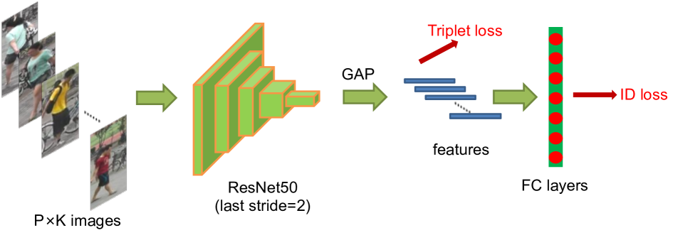
We follow a widely used open-source222https://github.com/Cysu/open-reid as our standard baseline. The backbone of the standard baseline is ResNet50 [5]. During the training stage, the pipeline includes following steps:
-
1.
We initialize the ResNet50 with pre-trained parameters on ImageNet and change the dimension of the fully connected layer to . denotes the number of identities in the training dataset.
-
2.
We randomly sample identities and images of per person to constitute a training batch. Finally the batch size equals to . In this paper, we set and .
-
3.
We resize each image into pixels and pad the resized image 10 pixels with zero values. Then randomly crop it into a rectangular image.
-
4.
Each image is flipped horizontally with 0.5 probability.
-
5.
Each image is decoded into 32-bit floating point raw pixel values in . Then we normalize RGB channels by subtracting 0.485, 0.456, 0.406 and dividing by 0.229, 0.224, 0.225, respectively.
-
6.
The model outputs ReID features and ID prediction logits .
-
7.
ReID features is used to calculate triplet loss [6]. ID prediction logits is used to calculated cross entropy loss. The margin of triplet loss is set to be 0.3.
-
8.
Adam method is adopted to optimize the model. The initial learning rate is set to be 0.00035 and is decreased by 0.1 at the 40th epoch and 70th epoch respectively. Totally there are 120 training epochs.
3 Training Tricks
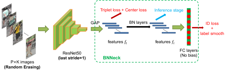
This section will introduce some effective training tricks in person ReID. Most of such tricks can be expanded on the standard baseline without changing the model architecture. The Fig. 2 (b) shows training strategies and the model architecture appeared in this section.
3.1 Warmup Learning Rate
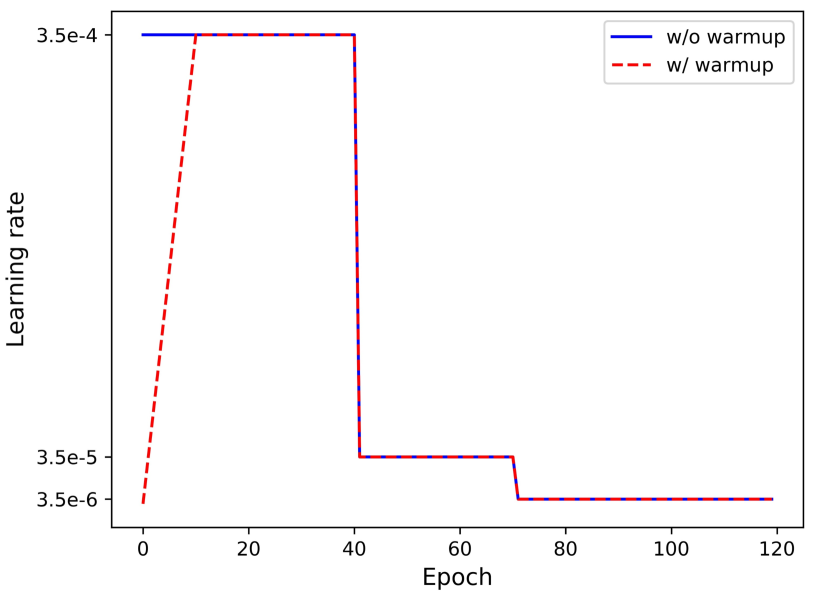
Learning rate has a great impact for the performance of a ReID model. Standard baseline is initially trained with a large and constant learning rate. In [2], a warmup strategy is applied to bootstrap the network for better performance. In practice, As shown in Fig. 3, we spent 10 epochs linearly increasing the learning rate from to . Then, the learning rate is decayed to and at 40th epoch and 70th epoch respectively. The learning rate at epoch is compute as;
| (1) |
3.2 Random Erasing Augmentation
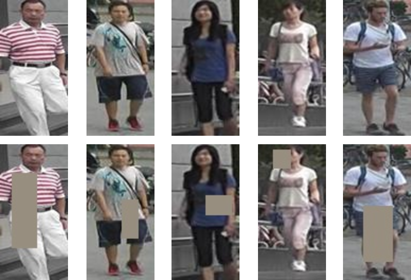
In person ReID, persons in the images are sometimes occluded by other objects. To address the occlusion problem and improve the generalization ability of ReID models, Zhong et al. [27] proposed a new data augmentation approach named as Random Erasing Augmentation (REA). In practice, for an image in a mini-batch, the probability of it undergoing Random Erasing is , and the probability of it being kept unchanged is . Then, REA randomly selects a rectangle region with size in image , and erases its pixels with random values. Assuming the area of image and region are and respectively, we denote as the area ratio of erasing rectangle region. In addition, the aspect ratio of region is randomly initialized between and . To determine a unique region, REA randomly initializes a point . If and , we set the region, , as the selected rectangle region. Otherwise we repeat the above process until an appropriate is selected. With the selected erasing region , each pixel in is assigned to the mean value of image , respectively.
In this study, we set hyper-parameters to , respectively. Some examples are shown in Fig. 4.
3.3 Label Smoothing
ID Embedding (IDE) [25] network is a basic baseline in person ReID. The last layer of IDE, which outputs the ID prediction logits of images, is a fully-connected layer with a hidden size being equal to numbers of persons . Given an image, we denote as truth ID label and as ID prediction logits of class . The cross entropy loss is computed as:
| (2) |
Because the category of the classification is determined by the person ID, we call such loss function as ID loss in this paper.
Nevertheless, person ReID can be regard as one-shot learning task because person IDs of the testing set have not appeared in the training set. So it is pretty important to prevent the ReID model from overfitting training IDs. Label smoothing (LS) proposed in [17] is a widely used method to prevent overfitting for a classification task. It changes the construction of to:
| (3) |
where is a small constant to encourage the model to be less confident on the training set. In this study, is set to be . When the training set is not very large, LS can significantly improve the performance of the model.
3.4 Last Stride
Higher spatial resolution always enriches the granularity of feature. In [16], Sun et al. removed the last spatial down-sampling operation in the backbone network to increase the size of the feature map. For convenience, we denote the last spatial down-sampling operation in the backbone network as last stride. The last stride of ResNet50 is set to be 2. When fed into a image of size, the backbone of ResNet50 outputs a feature map with the spatial size of . If change last stride from 2 to 1, we can get a feature map with higher spatial size (). This manipulation only increases very light computation cost and does not involve extra training parameters. However, higher spatial resolution brings significant improvement.
3.5 BNNeck
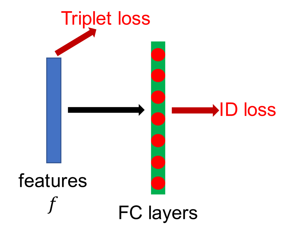
Most of works combined ID loss and triplet loss together to train ReID models. As shown in Fig. 5(a), in the standard baseline, ID loss and triplet loss constrain the same feature . However, the targets of these two losses are inconsistent in the embedding space.
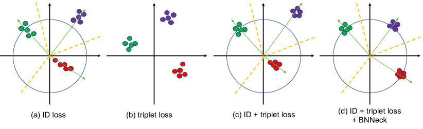
As shown in Fig. 6(a), ID loss constructs several hyperplanes to separate the embedding space into different sub-spaces. The features of each class are distributed in different subspaces. In this case, cosine distance is more suitable than Euclidean distance for the model optimized by ID loss in the inference stage. On the other hand, as shown in 6(b), triplet loss enhances the intra-class compactness and inter-class separability in the Euclidean space. Because triplet loss can not provide globally optimal constraint, inter-class distance sometimes is smaller than intra-class distance. A widely used method is to combine ID loss and triplet loss to train the model together. This approach let the model learn more discriminative features. Nevertheless, for image pairs in the embedding space, ID loss mainly optimizes the cosine distances while triplet loss focuses on the Euclidean distances. If we use these two losses to simultaneously optimize a feature vector, their goals may be inconsistent. In the training process, a possible phenomenon is that one loss is reduced, while the other loss is oscillating or even increased.
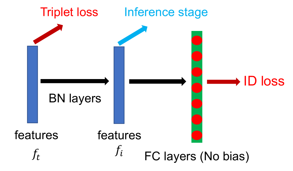
To overcome the aforementioned problem, we design a structure named as BNNeck shown in Fig. 5(b). BNNeck only adds a batch normalization (BN) layer after features (and before classifier FC layers). The feature before the BN layer is denoted as . We let pass through a BN layer to acquire the normalized feature . In the training stage, and are used to compute triplet loss and ID loss, respectively. Normalization balances each dimension of . The features are gaussianly distributed near the surface of the hypersphere. This distribution makes the ID loss easier to converge. In addition, BNNeck reduces the constraint of the ID loss on . Less constraint from ID loss leads to triplet loss easier to converge at the same time. Thirdly, normalization keeps the compact distribution of features that belong to one same person.
Because the hypersphere is almost symmetric about the origin of the coordinate axis, another trick of BNNeck is removing the bias of classifier FC layer. It constrains the classification hyperplanes to pass through the origin of the coordinate axis. We initialize the FC layer with Kaiming initialization proposed in [4].
In the inference stage, we choose to do the person ReID task. Cosine distance metric can achieve better performance than Euclidean distance metric. Experimental results in Table. 1 show that BNNeck can improve performance of the ReID model by a large margin.
3.6 Center Loss
Triplet loss is computed as:
| (4) |
where and are feature distances of positive pair and negative pair. is the margin of triplet loss, and equals to . In this paper, is set to . However, triplet loss only considers the difference between and and ignores the absolute values of them. For instance, when , the triplet loss is . For another case, when , the triplet loss also is . Triplet loss is determined by two person IDs sampled randomly. It is difficult to ensure that in the whole training dataset.
Center loss [20], which simultaneously learns a center for deep features of each class and penalizes the distances between the deep features and their corresponding class centers, makes up for the drawbacks of the triplet loss. The center loss function is formulated as:
| (5) |
where is the label of the th image in a mini-batch. denotes the th class center of deep features. is the number of batch size. The formulation effectively characterizes the intra-class variations. Minimizing center loss increases intra-class compactness. Our model totally includes three losses as follow:
| (6) |
is the balanced weight of center loss. In our experiments, is set to be .
4 Experimental Results
In this section, we will evaluate our models on Market1501 and DukeMTMC-reID [11] datasets. The Rank-1 accuracy and mean Average Precision (mAP) are reported as evaluation metrics. We add tricks on the standard baseline successively and do not change any training settings. The results of ablation studies present the performance boost from each trick. In order to prevent being misled by overfitting, we also show the results of cross-domain experiments.
4.1 Influences of Each Trick (Same domain)
| Market1501 | DukeMTMC | |||
|---|---|---|---|---|
| Model | r = 1 | mAP | r = 1 | mAP |
| Baseline-S | 87.7 | 74.0 | 79.7 | 63.7 |
| +warmup | 88.7 | 75.2 | 80.6 | 65.1 |
| +REA | 91.3 | 79.3 | 81.5 | 68.3 |
| +LS | 91.4 | 80.3 | 82.4 | 69.3 |
| +stride=1 | 92.0 | 81.7 | 82.6 | 70.6 |
| +BNNeck | 94.1 | 85.7 | 86.2 | 75.9 |
| +center loss | 94.5 | 85.9 | 86.4 | 76.4 |
The standard baseline introduced in section 2 achieves 87.7% and 79.7% rank-1 accuracies on Market1501 and DukeMTMC-reID, respectively. The performance of standard baseline is similar with most of baselines reported in other papers. Then, we add warmup strategy, random erasing augmentation, label smoothing, stride change, BNNeck and center loss to the model training process, one by one. Our designed BNNeck boosts more performance than other tricks, especially on DukeMTMC-reID. Finally, these tricks make baseline acquire 94.5% rank-1 accuracy and 85.9% mAP on Market1501. On DukeMTMC-reID, it reaches 86.4% rank-1 accuracy and 76.4% mAP. In other works, these training tricks boost the performance of the standard baseline by more than 10% mAP. In addition, to get such improvement, we only involve an extra BN layer and do not increase training time.
4.2 Analysis of BNNeck
| Market1501 | DukeMTMC | ||||
|---|---|---|---|---|---|
| Feature | Metric | r = 1 | mAP | r = 1 | mAP |
| (w/o BNNeck) | Euclidean | 92.0 | 81.7 | 82.6 | 70.6 |
| Euclidean | 94.2 | 85.5 | 85.7 | 74.4 | |
| Cosine | 94.2 | 85.7 | 85.5 | 74.6 | |
| Euclidean | 93.8 | 83.7 | 86.6 | 73.0 | |
| Cosine | 94.1 | 85.7 | 86.2 | 75.9 | |
In this section, we evaluate the performance of two different features ( and ) with Euclidean distance metric and cosine distance metric. All models are trained without center loss in Table. 2. We observe that cosine distance metric performs better than Euclidean distance metric for . Because ID loss directly constrains the features followed the BN layer, can be separated by several hyperplanes clearly. The cosine distance can measure the angle between two feature vectors, so cosine distance metric is more suitable than Euclidean distance metric for . However, is close to triplet loss and is constrained by ID loss at the same time. Two kinds of metrics achieve similar performance for .
In overall, BNNeck significantly improve the performance of ReID models. We choose with cosine distance metric to do the retrieval in the inference stage.
4.3 Influences of Each Trick (Cross domain)
| MD | DM | |||
|---|---|---|---|---|
| Model | r = 1 | mAP | r = 1 | mAP |
| Baseline | 24.4 | 12.9 | 34.2 | 14.5 |
| +warmup | 26.3 | 14.1 | 39.7 | 17.4 |
| +REA | 21.5 | 10.2 | 32.5 | 13.5 |
| +LS | 23.2 | 11.3 | 36.5 | 14.9 |
| +stride=1 | 23.1 | 11.8 | 37.1 | 15.4 |
| +BNNeck | 26.7 | 15.2 | 47.7 | 21.6 |
| +center loss | 27.5 | 15.0 | 47.4 | 21.4 |
| -REA | 41.4 | 25.7 | 54.3 | 25.5 |
To further explore effectiveness, we also present the results of cross-domain experiments in Table. 3. In overview, three tricks including warmup strategy, label smoothing and BNNeck significantly boost the cross-domain performance of ReID models. Stride change and center loss seem to have no big impact on the performance. However, REA does harm to models in cross-domain ReID task. In particularly, when our modified baseline is trained without REA, it achieves 41.4% and 54.3% rank-1 accuracies on Market1501 and DukeMTMC-reID datasets, respectively. Its performance surpass the ones of the standard baseline by a large margin. We infer that REA masking the regions of training images lets the model learn more knowledge in the training domain. It causes the model to perform worse in the testing domain.
4.4 Comparison of State-of-the-Arts
| Market1501 | DukeMTMC | |||||
|---|---|---|---|---|---|---|
| Type | Method | r = 1 | mAP | r = 1 | mAP | |
| Pose-guided | GLAD[19] | 4 | 89.9 | 73.9 | - | - |
| PIE [23] | 3 | 87.7 | 69.0 | 79.8 | 62.0 | |
| PSE [13] | 3 | 78.7 | 56.0 | - | - | |
| Mask-guided | SPReID [7] | 5 | 92.5 | 81.3 | 84.4 | 71.0 |
| MaskReID [9] | 3 | 90.0 | 75.3 | 78.8 | 61.9 | |
| Stripe-based | AlignedReID [21] | 1 | 90.6 | 77.7 | 81.2 | 67.4 |
| SCPNet [3] | 1 | 91.2 | 75.2 | 80.3 | 62.6 | |
| PCB [16] | 6 | 93.8 | 81.6 | 83.3 | 69.2 | |
| Pyramid[22] | 1 | 92.8 | 82.1 | - | - | |
| Pyramid[22] | 21 | 95.7 | 88.2 | 89.0 | 79.0 | |
| BFE[1] | 2 | 94.5 | 85.0 | 88.7 | 75.8 | |
| Attention-based | Mancs [18] | 1 | 93.1 | 82.3 | 84.9 | 71.8 |
| DuATM [14] | 1 | 91.4 | 76.6 | 81.2 | 62.3 | |
| HA-CNN [8] | 4 | 91.2 | 75.7 | 80.5 | 63.8 | |
| GAN-based | Camstyle [28] | 1 | 88.1 | 68.7 | 75.3 | 53.5 |
| PN-GAN [10] | 9 | 89.4 | 72.6 | 73.6 | 53.2 | |
| Global feature | IDE [25] | 1 | 79.5 | 59.9 | - | - |
| SVDNet [15] | 1 | 82.3 | 62.1 | 76.7 | 56.8 | |
| TriNet[6] | 1 | 84.9 | 69.1 | - | - | |
| AWTL[12] | 1 | 89.5 | 75.7 | 79.8 | 63.4 | |
| Ours | 1 | 94.5 | 85.9 | 86.4 | 76.4 | |
| Ours(RK) | 1 | 95.4 | 94.2 | 90.3 | 89.1 | |
We compare out strong baseline with state-of-the-arts methods in Table. 4. All methods have been divided into different types. Pyramid[22] achieves surprising performance on two datasets. However, it concatenates 21 local features of different scale. If only utilizing the global feature, it obtains 92.8% rank-1 accuracy and 82.1% mAP on Market1501. Ours strong baseline can reach 94.5% rank-1 accuracy and 85.9% mAP on Market1501. BFE[1] obtains similar performance with our strong baseline. But it combines features of two branches. Throughout all methods that only use global features, our strong baseline beats AWTL[12] by more than 10% mAP on both Market1501 and DukeMTMC-reID. With -reciprocal re-ranking method to boost the performance, our method reaches 94.1% mAP and 89.1% mAP on Market1501 and DukeMTMC-reID, respectively. To our best knowledge, our baseline achieves best performance in the case of only using global features.
5 Supplementary Experiments
We observed that some previous works were done with different the numbers of batch size or image sizes. In this section, as a supplementary we explore the affects of them on model performance.
5.1 Influences of the Number of Batch Size
| Batch Size | Market1501 | DukeMTMC | ||
|---|---|---|---|---|
| r = 1 | mAP | r = 1 | mAP | |
| 92.6 | 79.2 | 84.4 | 68.1 | |
| 92.9 | 80.0 | 84.7 | 69.4 | |
| 93.5 | 81.6 | 85.1 | 70.7 | |
| 93.9 | 82.0 | 85.8 | 71.5 | |
| 93.8 | 83.1 | 86.8 | 72.1 | |
| 93.8 | 83.7 | 86.6 | 73.0 | |
| 94.0 | 82.8 | 85.1 | 69.9 | |
| 93.1 | 81.6 | 86.7 | 72.1 | |
| 94.5 | 84.1 | 86.0 | 71.4 | |
| 93.2 | 82.8 | 86.5 | 73.1 | |
The mini-batch of triplet loss includes images. and denote the number of different persons and the number of different images per person, respectively. A mini-batch can only contain up to 128 images in one GPU, so that we can not do the experiments with or . We removed center loss to clearly find the relation between triplet loss and batch size. The results are present in Table. 5. However, there are not specific conclusions to show the effect of on performance. A slight trend we observed is that larger batch size is beneficial for the model performance. We infer that large helps to mine hard positive pairs while large helps to mining hard negative pairs.
5.2 Influences of Image Size
| Market1501 | DukeMTMC | |||
|---|---|---|---|---|
| Image Size | r = 1 | mAP | r = 1 | mAP |
| 93.8 | 83.7 | 86.6 | 73.0 | |
| 94.2 | 83.3 | 86.1 | 72.2 | |
| 94.0 | 82.7 | 86.4 | 73.2 | |
| 93.8 | 83.1 | 87.1 | 72.9 | |
We trained models without center loss and set . As shown in Table. 6, four models achieve similar performances on both datasets. In our opinion, the image size is not a pretty importance factor for the performance of ReID models.
6 Conclusions and Outlooks
In this paper, we collect some effective training tricks and design a strong baseline for person ReID. To demonstrate the influences of each trick on the performance of ReID models, we do a lot of experiments on both same-domain and cross-domain ReID tasks. Finally, only using global features, our strong baseline achieve 94.5% rank-1 accuracy and 85.9% mAP on Market1501. We hope that this work can promote the ReID research in academia and industry.
However, the purpose of our work is not to improve performance roughly. Compared with face recognition, person ReID still has a long way to explore. We think some training tricks can speed up the exploration and there are many effective tricks not discovered. We welcome researchers to share some other effective tricks with us. We will evaluate them based on this work.
In the future, we will continue to design more experiments to analyze the principles of these trciks. For example, when we replace the BNNeck with L2 normalization, what does the performance of this network become? In addition, whether can some state-of-the-arts methods such as PCB, MGN and AlignedReID, etc. be expanded on our strong baseline? More visualization also is helpful for others to understand this work.
7 Acknowledge
This work is supported by the National Natural Science Foundation of China (No. 61633019) and the Science Foundation of Chinese Aerospace Industry (JCKY2018204B053).
References
- [1] Zuozhuo Dai, Mingqiang Chen, Siyu Zhu, and Ping Tan. Batch feature erasing for person re-identification and beyond. arXiv preprint arXiv:1811.07130, 2018.
- [2] Xing Fan, Wei Jiang, Hao Luo, and Mengjuan Fei. Spherereid: Deep hypersphere manifold embedding for person re-identification. Journal of Visual Communication and Image Representation, 2019.
- [3] Xing Fan, Hao Luo, Xuan Zhang, Lingxiao He, Chi Zhang, and Wei Jiang. Scpnet: Spatial-channel parallelism network for joint holistic and partial person re-identification. arXiv preprint arXiv:1810.06996, 2018.
- [4] Kaiming He, Xiangyu Zhang, Shaoqing Ren, and Jian Sun. Delving deep into rectifiers: Surpassing human-level performance on imagenet classification. In Proceedings of the IEEE international conference on computer vision, pages 1026–1034, 2015.
- [5] Kaiming He, Xiangyu Zhang, Shaoqing Ren, and Jian Sun. Deep residual learning for image recognition. In Proceedings of the IEEE conference on computer vision and pattern recognition, pages 770–778, 2016.
- [6] Alexander Hermans, Lucas Beyer, and Bastian Leibe. In defense of the triplet loss for person re-identification. arXiv preprint arXiv:1703.07737, 2017.
- [7] Mahdi M Kalayeh, Emrah Basaran, Muhittin Gökmen, Mustafa E Kamasak, and Mubarak Shah. Human semantic parsing for person re-identification. In Proceedings of the IEEE Conference on Computer Vision and Pattern Recognition, pages 1062–1071, 2018.
- [8] Wei Li, Xiatian Zhu, and Shaogang Gong. Harmonious attention network for person re-identification. In Proceedings of the IEEE Conference on Computer Vision and Pattern Recognition, pages 2285–2294, 2018.
- [9] Lei Qi, Jing Huo, Lei Wang, Yinghuan Shi, and Yang Gao. Maskreid: A mask based deep ranking neural network for person re-identification. arXiv preprint arXiv:1804.03864, 2018.
- [10] Xuelin Qian, Yanwei Fu, Tao Xiang, Wenxuan Wang, Jie Qiu, Yang Wu, Yu-Gang Jiang, and Xiangyang Xue. Pose-normalized image generation for person re-identification. In Proceedings of the European Conference on Computer Vision (ECCV), pages 650–667, 2018.
- [11] Ergys Ristani, Francesco Solera, Roger Zou, Rita Cucchiara, and Carlo Tomasi. Performance measures and a data set for multi-target, multi-camera tracking. In European Conference on Computer Vision workshop on Benchmarking Multi-Target Tracking, 2016.
- [12] Ergys Ristani and Carlo Tomasi. Features for multi-target multi-camera tracking and re-identification. In Proceedings of the IEEE Conference on Computer Vision and Pattern Recognition, pages 6036–6046, 2018.
- [13] M. Saquib Sarfraz, Arne Schumann, Andreas Eberle, and Rainer Stiefelhagen. A pose-sensitive embedding for person re-identification with expanded cross neighborhood re-ranking. In The IEEE Conference on Computer Vision and Pattern Recognition (CVPR), June 2018.
- [14] Jianlou Si, Honggang Zhang, Chun-Guang Li, Jason Kuen, Xiangfei Kong, Alex C Kot, and Gang Wang. Dual attention matching network for context-aware feature sequence based person re-identification. In Proceedings of the IEEE Conference on Computer Vision and Pattern Recognition, pages 5363–5372, 2018.
- [15] Yifan Sun, Liang Zheng, Weijian Deng, and Shengjin Wang. Svdnet for pedestrian retrieval. In Proceedings of the IEEE International Conference on Computer Vision, pages 3800–3808, 2017.
- [16] Yifan Sun, Liang Zheng, Yi Yang, Qi Tian, and Shengjin Wang. Beyond part models: Person retrieval with refined part pooling (and a strong convolutional baseline). In Proceedings of the European Conference on Computer Vision (ECCV), pages 480–496, 2018.
- [17] Christian Szegedy, Vincent Vanhoucke, Sergey Ioffe, Jon Shlens, and Zbigniew Wojna. Rethinking the inception architecture for computer vision. In Proceedings of the IEEE conference on computer vision and pattern recognition, pages 2818–2826, 2016.
- [18] Cheng Wang, Qian Zhang, Chang Huang, Wenyu Liu, and Xinggang Wang. Mancs: A multi-task attentional network with curriculum sampling for person re-identification. In Proceedings of the European Conference on Computer Vision (ECCV), pages 365–381, 2018.
- [19] Longhui Wei, Shiliang Zhang, Hantao Yao, Wen Gao, and Qi Tian. Glad: Global-local-alignment descriptor for pedestrian retrieval. In Proceedings of the 25th ACM international conference on Multimedia, pages 420–428. ACM, 2017.
- [20] Yandong Wen, Kaipeng Zhang, Zhifeng Li, and Yu Qiao. A discriminative feature learning approach for deep face recognition. In European conference on computer vision, pages 499–515. Springer, 2016.
- [21] Xuan Zhang, Hao Luo, Xing Fan, Weilai Xiang, Yixiao Sun, Qiqi Xiao, Wei Jiang, Chi Zhang, and Jian Sun. Alignedreid: Surpassing human-level performance in person re-identification. arXiv preprint arXiv:1711.08184, 2017.
- [22] Feng Zheng, Xing Sun, Xinyang Jiang, Xiaowei Guo, Zongqiao Yu, and Feiyue Huang. A coarse-to-fine pyramidal model for person re-identification via multi-loss dynamic training. arXiv preprint arXiv:1810.12193, 2018.
- [23] Liang Zheng, Yujia Huang, Huchuan Lu, and Yi Yang. Pose invariant embedding for deep person re-identification. arXiv preprint arXiv:1701.07732, 2017.
- [24] Liang Zheng, Liyue Shen, Lu Tian, Shengjin Wang, Jingdong Wang, and Qi Tian. Scalable person re-identification: A benchmark. In Computer Vision, IEEE International Conference, 2015.
- [25] Zhedong Zheng, Liang Zheng, and Yi Yang. A discriminatively learned cnn embedding for person reidentification. ACM Transactions on Multimedia Computing, Communications, and Applications (TOMM), 14(1):13, 2018.
- [26] Zhun Zhong, Liang Zheng, Donglin Cao, and Shaozi Li. Re-ranking person re-identification with k-reciprocal encoding. In Proceedings of the IEEE Conference on Computer Vision and Pattern Recognition, pages 1318–1327, 2017.
- [27] Zhun Zhong, Liang Zheng, Guoliang Kang, Shaozi Li, and Yi Yang. Random erasing data augmentation. arXiv preprint arXiv:1708.04896, 2017.
- [28] Zhun Zhong, Liang Zheng, Zhedong Zheng, Shaozi Li, and Yi Yang. Camstyle: A novel data augmentation method for person re-identification. IEEE Transactions on Image Processing, 28(3):1176–1190, 2019.