Sensing Kondo correlations in a suspended carbon nanotube mechanical resonator with spin-orbit coupling

Abstract

We study electron mechanical coupling in a suspended carbon nanotube (CNT) quantum dot device. Electron spin couples to the flexural vibration mode due to spin-orbit coupling in the electron tunneling processes. In the weak coupling limit, i.e. electron-vibration coupling is much smaller than electron energy scale, the damping and resonant frequency shift of the CNT resonator can be obtained by calculating the dynamical spin susceptibility. We find that strong spin-flip scattering processes in Kondo regime significantly affect the mechanical motion of the carbon nanotube: Kondo effect induces strong damping and frequency shift of the CNT resonator.

I Introduction and short summary

Carbon nanotubes (CNTs) have been considered as an ideal platform for quantum dot (QD) devices Tans et al. (1997); Kouwenhoven and et al. (1997), which show Coulomb blockade oscillations, Luttinger liquid behavior Bockrath et al. (1999), Kondo effects Nygard et al. (2000); Jarillo-Herrero et al. (2005), and phase transitions Mebrahtu et al. (2012); Wang et al. (2010). CNTs is also emerging as a promising material for high-quality quantum nanomechanical applications Sapmaz et al. (2003); Sazonova et al. (2004); Garcia-Sanchez et al. (2007); Huttel et al. (2009); Lassagne et al. (2009); Steele et al. (2009); Moser et al. (2013, 2014a) due to their low mass and high stiffnesses, and thus is useful in quantum sensing Ares et al. (2016); Khosla et al. (2018); Degen et al. (2017), and in quantum information processing Pályi et al. (2012); Ohm et al. (2012); Rips and Hartmann (2013); Li et al. (2016). The strong coupling between mechanical vibrations and the electronic degree of freedom was achieved in high quality suspended CNT QD resonators Lassagne et al. (2009); Steele et al. (2009), when single electron tunnelings through the CNT QD are turned on. This electron-vibration coupling provides an opportunity to study the electron correlations and quantum noise through the measurement of the vibration of CNT resonator, and provides a way to achieve the electron-induced cooling of the resonator. Indeed, strong damping, frequency shift, and their nonlinearity effects of the CNT resonator are observed Lassagne et al. (2009); Steele et al. (2009).

In those observations, the electron-vibration coupling is induced by gate capacitance dependence of the resonator displacement, which only results in the coupling between the electron density and the vibrations. Therefore, Kondo effects, caused by spin-flip scatterings due to strong effective spin exchange coupling in low temperature Hewson (1997), seem to be irrelevant when considering mechanical effects. However, a recent theoretical proposal Rudner and Rashba (2011) shows that the coupling between the flexural vibration mode and the electron spin can be achieved in CNT, because the spin-orbit coupling in CNT Ando (2000); Huertas-Hernando et al. (2006); Kuemmeth et al. (2008); Steele et al. (2013) tends to align the spin with the tangent direction of CNT. Most interestingly, Kondo effects become relevant due to such spin-vibration coupling ($\Delta_{SO}$): Strong spin-flip scattering processes in Kondo regime might significantly affect the CNT vibrations. Therefore, CNT resonator may also provide a way to ”sensing” those quantum many body correlations.

In this work, we study a suspended CNT QD coupled to source-drain leads in the Kondo regime. Both the electron density-vibration coupling due to gate capacitance change and the spin-vibration coupling due to spin-orbit coupling are considered. When those couplings are much smaller than an electron energy scale (Kondo temperature), a perturbation treatment shows that the damping $\gamma$ and resonant frequency ($\omega_{0}$) shift of the CNT resonator due to electron (both density and spin) vibration coupling can be directly connected to the dynamical charge and spin susceptibilities. In the experimental realizable regime $\omega_{0}\sim T_{K}^{SU(2)}\ll\Delta_{KK^{\prime}}\ll\Delta_{SO}$ ($\Delta_{KK^{\prime}}$ is intervalley scattering), those dynamical susceptibilities can be obtained from non-crossing approximation Coleman (1984); Bickers et al. (1987); Brunner and Langreth (1997); Hewson (1997). We show that the strong spin-flip scatterings in Kondo regime induce strong damping and frequency shift of the CNT resonator. Those effects can be detected by using a finite frequency noise measurement Moser et al. (2013).

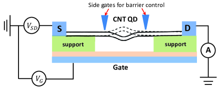
Figure 1: (color online) Schematics of the experimetal setup: a suspended doubly-clamped semiconducting CNT QD is connected by source and drain leads. Back gate is used to control the energy level of the QD, and the two side gates are for tunneling barrier control.

II Model and Hamiltonian

We consider a suspended doubly-clamped semiconducting CNT QD shown in Fig. 1. Due to the twofold real spin and twofold isospin symmetries, all the eigenenergies of the CNT quantum dot becomes fourfold degenerate Liang et al. (2002); Buitelaar et al. (2002). For each eigen-energy, the eigenstates can be written as $|\tau\,s\rangle=|\tau\rangle\otimes|s\rangle$, where $|\tau\rangle=|\frac{1}{2}\rangle,\,|-\frac{1}{2}\rangle$ represents the isospin and $|s\rangle=|\frac{1}{2}\rangle,\,|-\frac{1}{2}\rangle$ represents the real spin. The CNT also includes a spin-orbit coupling term and an intervalley scattering term, and the Hamiltonian is as follows

$$H_{{\rm CNT}}=H_{0}+\frac{\Delta_{SO}}{2}\tau_{3}(\textbf{s}\cdot\hat{\textbf{t}})+\Delta_{KK^{\prime}}\tau_{1}$$ (1)

where $H_{0}|\tau\,s\rangle=E_{0}|\tau\,s\rangle$, $\Delta_{SO}$ and $\Delta_{KK^{\prime}}$ are the spin-orbit coupling and the intervalley scattering, respectively. $\hat{\textbf{t}}=(t_{x},t_{y},t_{z})$ is the local tangent vector along the CNT axis, and we assume the CNT is along the $z$-direction without deformation. For the vibration, we focus on the lowest flexural mode, which can be described by a harmonic oscillator Ando (2000); Huertas-Hernando et al. (2006)

$$H_{\rm vib}=\frac{p^{2}}{2M}+\frac{1}{2}M\omega_{0}^{2}q^{2},$$ (2)

with CNT mass $M$, resonant frequency $\omega_{0}$, and the displacement $q$.

The flexural vibration of CNT QD couples to the electronic degree of freedom through two mechanisms: 1) the influence to the tangent vector which results in spin-vibration coupling Rudner and Rashba (2011); 2) the influence to the gate capacitance which induces the density-vibration coupling Sapmaz et al. (2003); Lassagne et al. (2009); Steele et al. (2009). For the first case, the flexural vibration (along $x$-direction) changes the tangent vector $\hat{\textbf{t}}$; and the vector becomes coordinate dependent $\hat{\textbf{t}}(z)=(\partial_{z}q/(\sqrt{1+(\partial_{z}q)^{2}}),0,1/(\sqrt{1+(\partial_{z}q)^{2}}))$. Up to second order of the small quantity $\partial_{z}q$, one has

$$\hat{\textbf{t}}(z)\backsimeq(1-(\partial_{z}q)^{2}/2)\hat{\textbf{z}}+\partial_{z}q\hat{\textbf{x}}.$$ (3)

The derivative of the displacement can be obtained: $\langle\partial_{z}q\rangle\sim\int_{-L/2}^{L/2}dz\,\rho(z)(df(z)/dz)$, where $\rho(z)$ is the electron density, $f(z)$ is the dimensionless wave function form, and $L$ is the length of the CNT. For symmetric quantum dot, the integral vanishes for even vibration mode. This cancellation can be avoided by introducing an asymmetric potential, considering odd vibration mode, or confining the electron only in part of the suspended CNTPályi et al. (2012). We choose last choice Pályi et al. (2012) for simplicity’s sake and obtain $\langle\partial_{z}q\rangle\backsimeq q/L$ and $\langle(\partial_{z}q)^{2}\rangle\backsimeq q^{2}/L^{2}$ (a constant pre-factor $\sim 1$ is dropped), the similar result can be obtained for other two choices. The nonlinear term in $\hat{\textbf{t}}(z)$ can be neglected since $q\ll L$. For the second case, the gate capacitance becomes a function of the displacement $q$: $C_{g}(q)=C_{g}^{0}+\partial_{q}C_{g}^{0}q+\partial_{q}^{2}C_{g}^{0}q^{2}/2+\cdots$ Sapmaz et al. (2003); Lassagne et al. (2009); Steele et al. (2009). Since $(\partial_{q}C_{g}^{0}q)/(\partial_{q}^{2}C_{g}^{0}q^{2}/2)\sim h/q\gg 1$ ( $h$ is the distance between CNT and the gate), the second and higher order terms can be neglected. We use a capacitor model to describe the electron-electron interaction, and in the presence of the vibration, we have

$$H_{\rm INT}=E_{c}(N-N_{g}^{0})^{2}-E_{c}\frac{2V_{g}}{e}\partial_{q}C_{g}^{0}Nq$$ (4)

where $E_{c}=e^{2}/(2C_{\sum})$ is the Coulomb charging energy with total capacitance $C_{\sum}=C_{L}+C_{R}+C_{g}$, $N$ is the electron number operator in QD, and $N_{g}=V_{g}C_{g}^{0}/2$ denotes the background charge with gate voltage $V_{g}$. For $T,V_{\rm SD}\ll\Delta<E_{c}$ ($T$, $V_{\rm SD}$, and $\Delta$ are temperature, source-drain voltage, and level spacing of QD), only a single energy level ($d$) near the Fermi level is relevant. The Hamiltonian of the CNT QD can be written as

$$H_{D} = E_{c}(N-N_{g}^{0})^{2}+\frac{p^{2}}{2M}+\frac{1}{2}M\omega_{0}^{2}q^{2}+\frac{\Delta_{SO}}{2}\tau_{3}s_{z}$$ (5)

$$+\Delta_{KK^{\prime}}\tau_{1}+\lambda_{D}N\,q+\lambda_{SO}\tau_{3}s_{x}\,q$$

where $N=\sum_{\sigma=\{s,\tau\}}d_{\sigma}^{\dagger}d_{\sigma}$, $\lambda_{SO}=\Delta_{SO}/L$, and $\lambda_{D}=-E_{c}2V_{g}\partial_{q}C_{g}^{0}/e$. The operator $d_{\sigma}$ annihilates a spin $\sigma$ electron in the CNT QD.

The CNT QD is coupled to two CNT leads, and the Hamiltonian for the whole system shown in Fig. 1 is

$$H = \sum_{\alpha=L/R}\sum_{k}\sum_{\sigma=\{s,\tau\}}\epsilon_{k,\sigma}c_{\alpha k,\sigma}^{\dagger}c_{\alpha k,\sigma}+H_{D}$$ (6)

$$\quad+\sum_{\alpha}\sum_{k}\sum_{\sigma=\{s,\tau\}}V_{\alpha k}\left(c_{\alpha k\sigma}^{\dagger}d_{\sigma}+h.c.\right)$$

where $c_{\alpha k,\sigma}$ annihilates an electron with momentum $k$ in the $\alpha$ lead with spin $\sigma$. $V_{\alpha k}$ describes the tunneling strength between CNT QD and the $\alpha$ lead, and can be controlled by two side gate shown in Fig. 1.

III Perturbation treatment for weak electron-vibration coupling

We want to study how the electron dynamics affect the physics of the resonator. For weak electron-vibration coupling ($\lambda_{SO},\lambda_{D}\ll\Gamma_{e}$), we treat $\lambda_{SO}$ and $\lambda_{D}$ as small parameter. Here, $\Gamma_{e}$ indicates the electron energy scale in the system, i.e. Kondo temperature in the Kondo regime, hybridization $\Gamma=\pi\rho_{0}|V_{L}|^{2}+\pi\rho_{0}|V_{R}|^{2}$ ($\rho_{0}$ is the electron density of state in the leads) in the mixed valence regime (i.e. the energy level of the dot $\epsilon_{d}$ is closed to the fermi level $|\epsilon_{d}|\ll\Gamma$).

The electron vibration coupling can be written in a general form $H_{\rm e-v}=h^{(1)}q$, where the linear coupling $h^{(1)}=\lambda_{D}N+\lambda_{SO}\tau_{3}s_{x}$ in our problem. For small coupling, the linear response theory results in

$$h^{(1)}(t)=h_{0}^{(1)}(t)-\int_{-\infty}^{\infty}\alpha_{h}^{(1)}(t^{\prime})q(t-t^{\prime})dt^{\prime}$$ (7)

where $\alpha_{h}^{(1)}(t-t^{\prime})=i\theta(t-t^{\prime})\langle[h^{(1)}(t),\;h^{(1)}(t^{\prime})]\rangle_{0}$ and $\langle\cdots\rangle_{0}$ indicates the average for system without electron-vibration coupling. By solving the Heisenberg equation of motion, we can obtain the equation describing the dynamics of the resonator in the linear response limit Dykman and Krivoglaz (1984)

$$\ddot{q}+2\gamma\dot{q}+\omega_{0}^{2}q=\frac{F}{M}\cos(\omega_{F}t)-\frac{h^{(1)}(t)}{M}$$ (8)

where we include a periodic driving force $F$ with frequency $\omega_{F}$, and a bare damping $\gamma=\omega_{0}/Q_{0}$ with quality factor $Q_{0}$. In the limit $\gamma,\,|\omega_{F}-\omega_{0}|\,\ll\omega_{0}$, one can analyze the problem in a rotating frame using the following transformation Dykman and Krivoglaz (1984)

$$q(t) = u(t)\,e^{i\omega_{F}t}+u^{*}(t)\,e^{-i\omega_{F}t}$$

$$\dot{q}(t) = i\omega_{F}\left(u(t)\,e^{i\omega_{F}t}-u^{*}(t)\,e^{-i\omega_{F}t}\right)$$ (9)

Combining Eq. (7), (8) and  (9), and then neglect the fast oscillating terms (like $e^{\pm i\omega_{F}t}$, $e^{\pm 2i\omega_{F}t}$, $\cdots$), the equation of motion for the resonator becomes Dykman and Krivoglaz (1984)

$$\dot{u}=-i\Big{[}\omega_{F}-\omega_{0}+\frac{{\rm Re}\Big{(}\alpha_{h}^{(1)}(\omega_{F})\Big{)}}{2M\omega_{F}}\Big{]}u$$ (10)

$$-\Big{[}\gamma+\frac{{\rm Im}\Big{(}\alpha_{h}^{(1)}(\omega_{F})\Big{)}}{2M\omega_{F}}\Big{]}u-i\frac{F}{4M\omega_{F}}+i\frac{h_{0}^{(1)}(t)}{2M\omega_{F}}e^{-i\omega_{F}t}.$$

One then obtain the damping ($\omega_{F}\approx\omega_{0}$) due to electron vibration coupling

$$\gamma^{e-v} =\gamma^{s-v}+\gamma^{d-v}=\frac{{\rm Im}\left[\alpha_{h}^{(1)}(\omega_{0})\right]}{2M\omega_{0}}$$

$$=\frac{\lambda_{SO}^{2}{\rm Im}[\chi_{\tau_{3}s_{x}}(\omega_{0})]}{2M\omega_{0}}+\frac{\lambda_{D}^{2}{\rm Im}\left[\chi_{N}(\omega_{0})\right]}{2M\omega_{0}},$$

where $\chi_{\tau_{3}s_{x}}(\omega)$ and $\chi_{N}(\omega)$ represent the dynamical spin susceptibility and density susceptibility respectively, which are the Fourier transforms of the functions $\chi_{\tau_{3}s_{x}}(t)=i\theta(t)\langle[\tau_{3}s_{x}(t),\tau_{3}s_{x}(0)]\rangle_{0}$ and $\chi_{N}(t)=i\langle[N(t),\;N(0)]\rangle_{0}$. We choose $\hbar=k_{B}=1$ throughout the paper. The frequency shift due to electron resonator interaction is

$$\Delta\omega^{s-v}=\frac{{\rm Re}\left[\alpha_{h}^{(1)}(\omega_{0})\right]}{2M\omega_{0}},$$ (12)

corresponding to the real part of the sum of the dynamical spin susceptibility and density susceptibility. The last term in Eq. (III) describes the noise.

In equilibrium, those susceptibilities are directly related to the spin and change fluctuations via fluctuation dissipation theorem. The fluctuations show different behaviors in different regimes. In the mixed valence regime ($|\epsilon_{d}|\ll\Gamma$), large charge and spin fluctuations Brunner and Langreth (1997); Lassagne et al. (2009); Steele et al. (2009) (i.e. electrons hop onto and off the CNT QD) induce large damping and frequency shift of the CNT resonator. The damping and frequency shift effects become weaker as temperature decreases. If energy level $\epsilon_{d}$ lays in the middle of conductance valley, electron tunnelings are blockaded. In low $T$ limit, this middle valley regime can be classified into two cases: 1) The total spin of QD is a singlet, 2) the total spin is a non-singlet. For the first case, no spin exchange coupling can be generated in low energy; and thus the fluctuations will be suppressed in low $T$ (with very small leftover due to quantum mechanical co-tunneling processes). For the second case, spin exchange coupling is generated in low $T$ and results in Kondo effects Hewson (1997) when $T<T_{K}$ ($T_{K}$ is called Kondo temperature). Kondo effects induce large spin fluctuations; and therefore, we expect large damping and frequency shift effects of the resonator in the regime $T\sim T_{K}$, and the effects become stronger as decreasing $T$. Although the charge fluctuations show an enhancement due to Kondo resonance, their value are much smaller than that of spin fluctuations Brunner and Langreth (1997). For $\lambda_{SO}\sim\lambda_{D}$, we can neglect the charge fluctuation part (i.e. the second term in Eq. (III)). We now focus on the spin fluctuation part in the Kondo regime in the rest of the paper.

IV Kondo regime

We want to calculate the the dynamical spin susceptibility $\chi_{\tau_{3}s_{x}}(\omega)$ of the system shown in Eq. (6) for $\lambda_{SO}=0$ and $\lambda_{D}=0$. For $\Delta_{SO}=0$ and $\Delta_{KK^{\prime}}=0$, this model shows $SU(4)$ Kondo effects Choi et al. (2005); Jarillo-Herrero et al. (2005) if the energy level is neither empty nor fully occupied (filled by 4 electrons). The large S-O interaction splits the four-fold degenerate spin states: $(1\uparrow,1\downarrow,2\uparrow,2\downarrow)$. Two lower energy states $(1\downarrow,2\uparrow)$ form a two-fold degenerate subspace, and two other states form another two-fold subspace as shown in Fig. 2 (a). For single occupied case, the system shows $SU(2)$ Kondo physics with two isospin states $(1\downarrow,2\uparrow)$ Galpin et al. (2010). For doubly occupied case, there is no Kondo effect. We have similar effects for triple occupied and fully occupied cases. If all the parameters ($E_{c}$, $\epsilon_{d}$, and $\Gamma$) are the same, we have $T_{K}^{SU(2)}\ll T_{K}^{SU(4)}$ Choi et al. (2005). The intervalley scatterings only generate the transitions $1\downarrow\leftrightarrow 2\downarrow$ or $2\uparrow\leftrightarrow 1\uparrow$, and thus do not affect the $SU(2)$ Kondo physics if $\Delta_{KK^{\prime}}\ll\Delta_{SO}$ (typical experimental value: $\Delta_{SO}=370\mu eV$ and $\Delta_{KK^{\prime}}=32.5\mu eV$ Kuemmeth et al. (2008)).

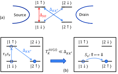
Figure 2: (color online) (a) Energy splitting due to spin orbit coupling. The blue cross arrows indicate the intervalley scatterings. (b) In the limit $T_{K}^{SU(2)}\ll\Delta_{KK^{\prime}}$, the operator $\tau_{3}s_{z}$ is equivalent to the operator $S_{x}$ in the lower subspace in the low energy. The coupling becomes $\frac{\lambda_{SO}q\,\Delta_{KK^{\prime}}}{\Delta_{SO}}=\lambda_{KK^{\prime}}q$.

We are interested in an experimentally realizable regime: $\lambda_{SO}q_{\rm amp}\ll\omega_{0}\sim T_{K}^{SU(2)}\ll T_{K}^{SU(4)}<\Delta_{KK^{\prime}}<\Delta_{SO}$, where $q_{\rm amp}$ is the amplitude of the vibration. If the system is in the middle of the single occupied valley, two isospin states $(1\downarrow,2\uparrow)=(\Downarrow,\Uparrow)$ along with the leads form a $SU(2)$ Kondo state. The Kondo effect enhances the spin-flip $\Downarrow\leftrightarrow\Uparrow$ scattering processes between two isospin states, and their time scale (between two adjacent spin-flip events) corresponds to $\tau_{{\rm SF}}\sim 1/T_{K}^{SU(2)}$. In the spin susceptibility, when the operator $\tau_{3}s_{x}$ is applied on the impurity state, the impurity state will immediately go to the higher energy subspace: from $1\downarrow$ to $1\uparrow$ (or from $2\downarrow$ to $2\uparrow$). The system will finally relax to the lower energy subspace through two possible scattering mechanism: 1) spin (real spin or isospin) exchange processes via dot-leads hopping, 2) intervalley scattering. The leading relaxation processes are the intervalley scatterings (time scale comparison: $1/\Delta_{KK^{\prime}}<1/T_{K}^{SU(4)}$). In addition, this relaxation time is much smaller than spin-flip time scale, i.e. $1/\Delta_{KK^{\prime}}\ll 1/T_{K}^{SU(2)}$. So, if we only consider the low energy physics $\omega\sim T_{K}^{SU(2)}$, the operator $\tau_{3}s_{x}$ along with the fast relaxation process just behave as the $S_{x}$ operator in the isospin subspace $(\Downarrow,\Uparrow)$ as demonstrated in Fig. (2) (b), and the vibration-spin coupling becomes $\frac{\lambda_{SO}\Delta_{KK^{\prime}}}{\Delta_{SO}}S_{x}q=\lambda_{KK^{\prime}}S_{x}q$ with $\lambda_{KK^{\prime}}=\Delta_{KK^{\prime}}/L$. In the low energy, the system will exhibit the $SU(2)$ rotation symmetry. When considering the low energy response $\omega\sim T_{K}^{SU(2)}$, we can safely neglect the $SU(2)$ symmetry breaking terms, and the spin $x$ response function are exactly the same as the spin $z$ response function. Therefore, our task is reduced to the standard problem: Calculating the response functions

$$\gamma^{s-v}=\frac{\lambda_{KK^{\prime}}^{2}{\rm Im}\left[\chi_{S_{z}}(\omega_{0})\right]}{2M\omega_{0}},\;\,\Delta\omega^{s-v}=\frac{\lambda_{KK^{\prime}}^{2}{\rm Re}\left[\chi_{S_{z}}(\omega_{0})\right]}{2M\omega_{0}}$$ (13)

for a two-fold degenerate Anderson model

$$H = \sum_{\alpha,k}\sum_{\sigma}\epsilon_{k,\sigma}c_{\alpha k,\sigma}^{\dagger}c_{\alpha k,\sigma}+\sum_{\sigma}\epsilon_{d}d_{\sigma}^{\dagger}d_{\sigma}+Ud_{\Uparrow}^{\dagger}d_{\Uparrow}d_{\Downarrow}^{\dagger}d_{\Downarrow}$$ (14)

$$+\sum_{\alpha k\sigma}V_{\alpha k}\left(c_{\alpha k\sigma}^{\dagger}d_{\sigma}+h.c.\right)\;.$$

where $\sigma=\{\Downarrow,\Uparrow\}$, $U=2E_{c}$, and $S_{z}=(d_{\Uparrow}^{\dagger}d_{\Uparrow}-d_{\Downarrow}^{\dagger}d_{\Downarrow})/2$.

V Damping and frequency shift due to Kondo correlation

We will calculate the damping and frequency shift of the CNT resonator due to electron-vibration coupling induced in the Kondo regime, i.e. Eq. (13) for Hamiltonian in Eq. (14). Although the exact result might be obtained from numerical techniques, e.g. numerical renormalization group, real-time quantum Monte Carlo techniques, analytic treatments are extremely non-trivial. Since spin-flip process can occur through the virtual processes involving either the empty state or the doubly occupied state, essential physics of the Kondo effect will not be significantly affected if one remove the doubly occupied state from the Hilbert space. To study the Kondo physics, one then can use the standard simplification, i.e. study an infinite-U (interaction) Anderson model. This model can be solved by using a standard non-crossing approximation (NCA) Coleman (1984); Bickers et al. (1987); Hewson (1997), which is exact for large degeneracy limit. But it can capture the essential physics for energy above a pathology scale $\sim 10^{-1}-10^{-2}T_{K}$ Bickers (1987); Hewson (1997) even for our $2$-fold degenerate case.

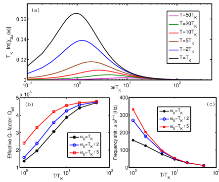
Figure 3: (color online) (a) The imaginary part of the dynamical spin susceptibility as a function of the frequency $\omega$ for $D=5.0$, $\Gamma=\Gamma_{L}+\Gamma_{R}=0.5$, and $\epsilon_{d}=-1.5$. From bottom to top: $T=50T_{K},\,\cdots,\,T_{K}$. (b) The effective quality factor, (c) the frequency shift of the CNT resonator. The parameters are shown in the text.

The Green function of problem can be obtained by solving a set of coupled integral equations iteratively Coleman (1984); Bickers et al. (1987); Hewson (1997) (also refer to Apendix app for more details about the calculation of dynamical spin susceptibility in Kondo regime). Fig. 3 (a) shows the imaginary part of the dynamical spin susceptibility $T_{K}\rm{Im}[\chi_{S_{z}}(\omega)]$ as a function of the frequency $\omega/T_{K}$ for different temperatures. We choose the parameters: electron lead band width $D=5.0$, $\Gamma=\Gamma_{L}+\Gamma_{R}=0.5$, and $\epsilon_{d}=-1.5$ such that the Kondo temperature $T_{K}\approx 0.01$ (this is obtained from the width of the impurity spectrum function). As expected Coleman (1984); Bickers et al. (1987); Brunner and Langreth (1997); Hewson (1997), a peak maximum appears in the susceptibility spectrum; and it is shifted to lower frequency and approaches $\omega=T_{K}$ as $T$ is lowered. The real part of the susceptibility spectrum is related to its imaginary part through Kramers-Kronig relation. We then calculate the effective quality factor $Q_{\rm eff}$, which is given as

$$\frac{\omega_{0}}{Q_{\rm eff}}=\frac{\omega_{0}}{Q_{0}}+\gamma_{s-v},$$ (15)

and the frequency shift $\Delta\omega_{s-v}$. We choose the following experimental realizable parameters Poot and van der Zant (2012); Moser et al. (2014b); Jespersen et al. (2011): bare quality factor $Q_{0}=4.8\times 10^{6}$, suspended CNT length and mass $L=1.8\mu m$ and $M=4.4\times 10^{-21}kg$, resonant frequency $\omega_{0}=2\pi f_{0}=2\pi\times 55.6MHz$, $\Delta_{KK^{\prime}}=200\mu eV$ (note that the intervalley scattering comes from disorder and their value fluctuates from device to device, Jespersen, et al. reported the value as large as $450\mu eV$.), and Kondo temperature $T_{K}=T_{K}^{SU(2)}=\omega_{0}$, $2\omega_{0}$, and $5\omega_{0}$. The effective electron-vibration coupling is estimated in their zero-point motion state $\lambda_{SO}q_{0}=\Delta_{SO}/(L\sqrt{2M\omega_{0}})\backsimeq 0.0028\omega_{0}\ll\omega_{0}$, which is small enough to justify the perturbation method. The effective quality factor and the frequency shift of the CNT resonator are shown in Fig. 3 (b) and (c). It is clear that as the $T$ is lowered and approaches the Kondo regime $T\sim T_{K}$, the strong spin-flip scatterings between CNT QD resonator and their leads, along with the spin-orbit interaction, induce a large damping effect and thus decrease the effective quality factor dramatically. The effective resonant frequency of the resonator is also affected by Kondo effect: The frequency shift increases as $T$ decreases.

The authors grateful to Y.Liu, A. Levchenko, M.I. Dykman and H.U.Baranger for valuable discussions. The authors acknowledge support from Thousand-Young-Talent program of China, and the startup grant from State Key Laboratory of Low-Dimensional Quantum Physics and Tsinghua University.

Appendix A Dynamical spin susceptibility

In this appendix, we will calculate the Kondo induced damping and frequency shift, i.e. Eq. (13) for the Hamiltonian shown in Eq. (14). Since spin-flip process can occur through both the virtual process involving the empty state and the virtual process involving the doubly occupied state, essential physics of the Kondo effect will not be significantly affected if one remove the doubly occupied state from the Hilbert space. To study the Kondo physics, one then can use the standard simplification, i.e. study an infinite-U (interaction) Anderson model instead of the finite-U Anderson model shown in Eq. (14). The Hamiltonian for N-fold degenerate model can be written as

$$H = \sum_{m=1}^{N}\sum_{\alpha k}\epsilon_{\alpha k}c_{\alpha km}^{\dagger}c_{\alpha km}+\epsilon_{d}\sum_{m=1}^{N}\hat{N}_{m}$$ (16)

$$+\sum_{\alpha k}\sum_{m}V_{\alpha k}\left(c_{\alpha km}^{\dagger}F_{m}+h.c.\right),$$

where $\hat{N}_{0}=|0\rangle\langle 0|$, $\hat{N}_{m}=|m\rangle\langle m|$, and $F_{m}=|0\rangle\langle m|$ ($\langle 0|$ represents the empty state and $\langle m|$ represents the occupied state). This model can be solved using a standard non-crossing approximation (NCA) Coleman (1984); Bickers et al. (1987); Hewson (1997) which neglect all the crossing diagram. This method is justified for large N limit, but still can capture the essential physics for energy above a pathology scale $\sim 10^{-1}-10^{-2}T_{K}$ Bickers (1987); Hewson (1997) even for $N=2$. The NCA method gives coupled integral equations Coleman (1984); Bickers et al. (1987); Hewson (1997) for the empty state propagator $G_{0}$ and occupied state propagator $G_{m}$

$$G_{0}(\omega) = \frac{1}{\omega-\Sigma_{0}(\omega)}$$ (17)

$$G_{m}(\omega) = \frac{1}{\omega-\epsilon_{d}-\Sigma_{m}(\omega)}$$ (18)

$$\Sigma_{0}(\omega) = \frac{N\Gamma}{\pi}\int_{-D}^{D}\frac{f(\omega)}{\omega+\epsilon-\epsilon_{d}-\Sigma_{m}(\omega+\epsilon)}d\epsilon$$ (19)

$$\Sigma_{m}(\omega) = \frac{\Gamma}{\pi}\int_{-D}^{D}\frac{1-f(\omega)}{\omega-\epsilon-\Sigma_{m}(\omega-\epsilon)}d\epsilon$$ (20)

Here $\Gamma=\Gamma_{L}+\Gamma_{R}$ ($\Gamma_{\alpha}=\pi|V_{\alpha}|^{2}\rho$) and $D$ is the half band width of the system. The coupled integral equation can be simply solved using iteration method. The empty-state spectrum and the occupied state spectrum are

$$\rho_{0}(\omega) = -\frac{1}{\pi}{\rm Im}G_{0}^{R}(\omega)$$ (21)

$$\rho_{m}(\omega) = -\frac{1}{\pi}{\rm Im}G_{m}^{R}(\omega)$$ (22)

Then, the physical observables, e.g. full impurity spectral function and the dynamical spin susceptibility can be obtained

$$A_{d}(\omega) = \frac{1}{Z_{f}}(1+e^{-\beta\omega})\int_{-\infty}^{\infty}d\epsilon\;e^{-\beta\epsilon}\rho_{0}(\epsilon)\rho_{m}(\epsilon+\omega)$$

$${\rm Im}\left[\chi_{S_{z}}(\omega)\right] = \frac{N\,j(j+1)}{3}\frac{\pi}{Z_{f}}\int_{-\infty}^{\infty}d\epsilon\;e^{-\beta\epsilon}\rho_{m}(\epsilon)$$ (23)

$$\times\left[\rho_{m}(\epsilon+\omega)-\rho_{m}(\epsilon-\omega)\right]$$

where $j=(N-1)/2$ and

$$Z_{f}=\int_{-\infty}^{\infty}d\epsilon\;e^{-\beta\epsilon}\left[\rho_{0}(\epsilon)+\sum_{m}\rho_{m}(\epsilon)\right].$$ (24)

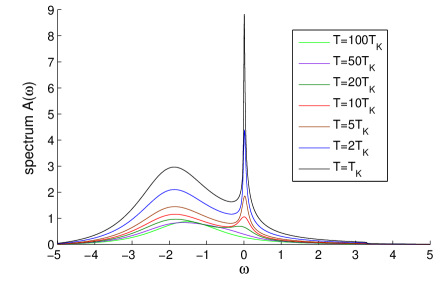
Figure 4: The impurity spectral function for different temperature.

For our problem, the degeneracy is $N=2$. We did a calculation for $D=5.0$, $\Gamma=0.5$, and $\epsilon_{d}=-1.5$, so that the Kondo temperature is $T_{K}\sim 0.01$ (this can be directly obtained from the width of the Kondo resonance of the impurity spectrum $A_{d}(\omega)$). We test the impurity spectral function for different temperature shown in Fig. 4, we can see that the narrow Kondo resonance around $\omega=0$ is developed for low temperature. We then obtain the dynamical spin susceptibility numerically as shown in Fig.3 of the main text.

References

- Tans et al. (1997) S. J. Tans, M. H. Devoret, H. Dai, A. Thess, R. E. Smalley, L. J. Geerligs, and C. Dekker, Nature 386, 474 (1997).
- Kouwenhoven and et al. (1997) L. P. Kouwenhoven and et al., in Mesoscopic Electron Transport s, edited by L. P. Kouwenhoven, G. Schon, and S. L. L. (Kluwer Academic Publishing, Dordrecht, 1997), p. 105.
- Bockrath et al. (1999) M. Bockrath, D. H. Cobden, J. Lu, A. G. Rinzler, R. E. Smalley, L. Balents, and P. L. McEuen, Nature 397, 598 EP (1999).
- Nygard et al. (2000) J. Nygard, D. H. Cobden, and P. E. Lindelof, Nature 408, 342 (2000).
- Jarillo-Herrero et al. (2005) P. Jarillo-Herrero, J. Kong, H. S. J. van der Zant, C. Dekker, L. P. Kouwenhoven, and S. De Franceschi, Nature 434, 484 (2005).
- Mebrahtu et al. (2012) H. T. Mebrahtu, I. V. Borzenets, D. E. Liu, H. Zheng, Y. V. Bomze, A. I. Smirnov, H. Baranger, and G. Finkelstein, Nature 488, 61 (2012).
- Wang et al. (2010) Z. Wang, J. Wei, P. Morse, J. G. Dash, O. E. Vilches, and D. H. Cobden, Science 327, 552 (2010), ISSN 0036-8075.
- Sapmaz et al. (2003) S. Sapmaz, Y. M. Blanter, L. Gurevich, and H. S. J. van der Zant, Phys. Rev. B 67, 235414 (2003).
- Sazonova et al. (2004) V. Sazonova, Y. Yaish, H. Ustunel, D. Roundy, T. A. Arias, and P. L. McEuen, Nature 431, 284 (2004).
- Garcia-Sanchez et al. (2007) D. Garcia-Sanchez, A. San Paulo, M. J. Esplandiu, F. Perez-Murano, L. Forró, A. Aguasca, and A. Bachtold, Phys. Rev. Lett. 99, 085501 (2007).
- Huttel et al. (2009) A. K. Huttel, G. A. Steele, B. Witkamp, M. Poot, L. P. Kouwenhoven, and H. S. J. van der Zant, Nano Letters 9, 2547 (2009).
- Lassagne et al. (2009) B. Lassagne, Y. Tarakanov, J. Kinaret, D. Garcia-Sanchez, and A. Bachtold, Science 325, 1107 (2009).
- Steele et al. (2009) G. A. Steele, A. K. H?tel, B. Witkamp, M. Poot, H. B. Meerwaldt, L. P. Kouwenhoven, and H. S. J. van der Zant, Science 325, 1103 (2009).
- Moser et al. (2013) J. Moser, J. Guttinger, A. Eichler, M. J. Esplandiu, D. E. Liu, M. I. Dykman, and A. Bachtold, Nature Nanotechnology 8, 493 (2013).
- Moser et al. (2014a) J. Moser, A. Eichler, J. Güttinger, M. I. Dykman, and A. Bachtold, Nature Nanotechnology 9, 1007 EP (2014a).
- Ares et al. (2016) N. Ares, T. Pei, A. Mavalankar, M. Mergenthaler, J. H. Warner, G. A. D. Briggs, and E. A. Laird, Phys. Rev. Lett. 117, 170801 (2016).
- Khosla et al. (2018) K. E. Khosla, M. R. Vanner, N. Ares, and E. A. Laird, Phys. Rev. X 8, 021052 (2018).
- Degen et al. (2017) C. L. Degen, F. Reinhard, and P. Cappellaro, Rev. Mod. Phys. 89, 035002 (2017).
- Pályi et al. (2012) A. Pályi, P. R. Struck, M. Rudner, K. Flensberg, and G. Burkard, Phys. Rev. Lett. 108, 206811 (2012).
- Ohm et al. (2012) C. Ohm, C. Stampfer, J. Splettstoesser, and M. R. Wegewijs, Applied Physics Letters 100, 143103 (pages 4) (2012).
- Rips and Hartmann (2013) S. Rips and M. J. Hartmann, Phys. Rev. Lett. 110, 120503 (2013).
- Li et al. (2016) P.-B. Li, Z.-L. Xiang, P. Rabl, and F. Nori, Phys. Rev. Lett. 117, 015502 (2016).
- Hewson (1997) A. Hewson, The Kondo problem to heavy fermions (Cambridge Univ. Press, 1997).
- Rudner and Rashba (2011) M. S. Rudner and E. I. Rashba, Phys. Rev. B 83, 073406 (2011).
- Ando (2000) T. Ando, Journal of the Physical Society of Japan 69, 1757 (2000).
- Huertas-Hernando et al. (2006) D. Huertas-Hernando, F. Guinea, and A. Brataas, Phys. Rev. B 74, 155426 (2006).
- Kuemmeth et al. (2008) F. Kuemmeth, S. Ilani, D. C. Ralph, and P. L. McEuen, Nature 452, 448 (2008).
- Steele et al. (2013) G. A. Steele, F. Pei, E. A. Laird, J. M. Jol, H. B. Meerwaldt, and L. P. Kouwenhoven, Nature Communications 4, 1573 (2013).
- Coleman (1984) P. Coleman, Phys. Rev. B 29, 3035 (1984).
- Bickers et al. (1987) N. E. Bickers, D. L. Cox, and J. W. Wilkins, Phys. Rev. B 36, 2036 (1987).
- Brunner and Langreth (1997) T. Brunner and D. C. Langreth, Phys. Rev. B 55, 2578 (1997).
- Liang et al. (2002) W. Liang, M. Bockrath, and H. Park, Phys. Rev. Lett. 88, 126801 (2002).
- Buitelaar et al. (2002) M. R. Buitelaar, A. Bachtold, T. Nussbaumer, M. Iqbal, and C. Schönenberger, Phys. Rev. Lett. 88, 156801 (2002).
- Dykman and Krivoglaz (1984) M. I. Dykman and M. A. Krivoglaz, in Sov. Phys. Reviews, edited by I. M. Khalatnikov (Harwood Academic, New York, 1984), pp. 265-441.
- Choi et al. (2005) M.-S. Choi, R. López, and R. Aguado, Phys. Rev. Lett. 95, 067204 (2005).
- Galpin et al. (2010) M. R. Galpin, F. W. Jayatilaka, D. E. Logan, and F. B. Anders, Phys. Rev. B 81, 075437 (2010).
- Bickers (1987) N. E. Bickers, Rev. Mod. Phys. 59, 845 (1987).
- Poot and van der Zant (2012) M. Poot and H. S. van der Zant, Physics Reports 511, 273 (2012).
- Moser et al. (2014b) J. Moser, A. Eichler, J. Guttinger, M. I. Dykman, and A. Bachtold, Nature Nanotechnology 9, 1007 (2014b).
- Jespersen et al. (2011) T. S. Jespersen, K. Grove-Rasmussen, J. Paaske, K. Muraki, T. Fujisawa, J. Nygard, and K. Flensberg, Nature Physics 7, 348 (2011).