Cross-correlation of Polarbear CMB Polarization Lensing with High-$z$ Sub-mm Herschel-ATLAS Galaxies

Abstract

We report a 4.8$\sigma$ measurement of the cross-correlation signal between the cosmic microwave background (CMB) lensing convergence reconstructed from measurements of the CMB polarization made by the Polarbear experiment and the infrared-selected galaxies of the Herschel-ATLAS survey. This is the first measurement of its kind. We infer a best-fit galaxy bias of $b=5.76\pm 1.25$, corresponding to a host halo mass of $\log_{10}(M_{h}/M_{\odot})=13.5^{+0.2}_{-0.3}$ at an effective redshift of $z\sim 2$ from the cross-correlation power spectrum. Residual uncertainties in the redshift distribution of the sub-mm galaxies are subdominant with respect to the statistical precision. We perform a suite of systematic tests, finding that instrumental and astrophysical contaminations are small compared to the statistical error. This cross-correlation measurement only relies on CMB polarization information that, differently from CMB temperature maps, is less contaminated by galactic and extragalactic foregrounds, providing a clearer view of the projected matter distribution. This result demonstrates the feasibility and robustness of this approach for future high-sensitivity CMB polarization experiments.

1 Introduction

The pattern of the cosmic microwave background (CMB) anisotropies not only provides a snapshot of the primordial universe at $z\approx 1100$, but also encodes a wealth of information about its evolution after recombination (e.g., Aghanim et al., 2008). In particular, the trajectory of CMB photons while traveling between the last-scattering surface and us can be deflected by the intervening matter distribution, an effect known as weak gravitational lensing (Lewis & Challinor, 2006). These deflections, typically of a few arcminutes, introduce correlations between modes of the CMB anisotropies that can be exploited to reconstruct the projected gravitational potential (CMB lensing potential $\phi$) in the whole observable universe (Hu & Okamoto, 2002; Hirata & Seljak, 2003). The sensitivity of the lensing signature to both the geometry and the growth of structures of the universe makes it suitable to break the geometrical degeneracy affecting the primary CMB (Stompor & Efstathiou, 1999) and to investigate the neutrino and dark sector.

Since its first detection about a decade ago (Smith et al., 2007; Kuo et al., 2007; Hirata et al., 2008), CMB lensing science has rapidly progressed and several collaborations have reported highly significant measurements of the CMB lensing power spectrum, including the ACT (Das et al., 2014; Sherwin et al., 2017, temperature and polarization), BICEP/Keck (BICEP2/Keck Array Collaboration, 2016, polarization-only), Planck (Planck Collaboration, 2014a, 2016a, 2018b, temperature and polarization), Polarbear (POLARBEAR Collaboration, 2014b, polarization-only), and SPT (Story et al., 2015; Omori et al., 2017, temperature and polarization) collaborations.

Given that CMB lensing probes the projected matter distribution along the line-of-sight up to very high redshifts, it is highly correlated with other tracers of large-scale structure (LSS) such as galaxies. Several groups have detected the cross-correlation signal between CMB lensing and galaxies selected in different wavelengths. Cosmological and astrophysical applications of the CMB lensing-galaxy clustering cross-correlations include the study of the galaxy bias evolution (e.g., Sherwin et al., 2012; Bleem et al., 2012; DiPompeo et al., 2014; Bianchini et al., 2015; Allison et al., 2015; Bianchini et al., 2016), the measurement of the growth of structure (e.g., Giannantonio et al., 2016; Pullen et al., 2016; Bianchini & Reichardt, 2018; Peacock & Bilicki, 2018; Omori et al., 2018), the calibration of cosmic shear measurements (Baxter et al., 2016), and the investigation of primordial non-Gaussianities (Giannantonio & Percival, 2014). Moreover, cross-correlations are becoming a standard probe to be included in the general cosmological parameters estimation framework (e.g., Abbott et al., 2018). The advantage of a cross-correlation analysis is twofold. First, cross-correlation allows one to separate the CMB lensing signal to a specific range of redshifts (the redshifts of the galaxy sample). Second, cross-correlations are less prone to systematic effects as most systematics will be uncorrelated between different experiments and wavelengths.

In this paper, we measure the cross-correlation between CMB lensing convergence maps $\kappa=-\frac{1}{2}\nabla^{2}\phi$ reconstructed by the Polarbear experiment and the clustering of bright sub-millimetre (sub-mm) galaxies detected by the Herschel satellite. Sub-mm galaxies are thought to undergo an intense phase of star-formation in a dust-rich environment, where ultraviolet light emitted by newly born stars is absorbed by the dust and subsequently re-emitted in the far-infrared (e.g., Smail et al., 1997; Blain et al., 2002). The brightest sub-mm galaxies can reach luminosities of about $10^{13}L_{\odot}$, with corresponding star-formation rates up to $\sim 1000\,M_{\odot}/$year.

A peculiarity of the spectral energy distribution (SED) of sub-mm galaxies is that there is a strongly negative $K$-correction at mm and sub-mm wavelengths, meaning that the observed sub-mm flux of such galaxies is nearly independent of redshift from $1\lesssim z\lesssim 8$ (for a recent review of dusty star-forming galaxies see Casey et al., 2014). Sub-mm galaxy samples are weighted towards high redshifts ($1\lesssim z\lesssim 3$), which is the redshift range where a given matter fluctuation will lead to the largest CMB lensing signal. Thus sub-mm galaxies are perfect candidates for CMB lensing-galaxy density cross-correlation studies.

The Cosmic Infrared Background (CIB) is thought to comprise the emission of unresolved infrared galaxies. It is then natural to expect a high degree of correlation with CMB lensing (Song et al., 2003). Recent studies have investigated the cross-correlation between CMB lensing and maps of the diffuse CIB (e.g. Holder et al., 2013; Planck Collaboration, 2014b; POLARBEAR Collaboration, 2014a; van Engelen et al., 2015; Planck Collaboration, 2018b), finding correlation coefficients up to 80% at about 500 $\mu$m.

Our analysis clearly shares some similarities with these studies because Herschel galaxies constitute part of the CIB, even though, despite having been extensively studied in recent years, the exact redshift distribution of contributions to the CIB is still debated (e.g., Casey et al., 2014, and references therein). CIB only provides an integrated measurement and thus, unlike the catalog-based approach adopted in this work, prevent any accurate redshift tomography of the cross-correlation signal to study the properties of sub-mm galaxies.

In the past, Bianchini et al. (2015, 2016) cross-correlated similar sub-mm Herschel catalogs with the 2013 and 2015 Planck CMB lensing maps, reporting a rejection of the no-correlation hypothesis between the two fields at the $\approx 20\sigma$ level. While Planck CMB lensing reconstruction is mostly dominated by the CMB temperature information, and hence more contaminated by galactic and extragalactic foregrounds, Polarbear CMB lensing convergence maps only rely on polarization data. This represents the first study of this kind and was made possible thanks to the depth of the Polarbear observations. With this sensitivity and Polarbear resolution, probes of cross-correlation signal at smaller scales have become accessible.

Polarbear map depth sensitivity is comparable to upcoming ground-based CMB experiments which will cover a much larger fraction of the sky. This work thus serves as a proof of concept that reliable cross-correlation measurements can indeed be achieved without CMB temperature information, providing a more robust measurement against galactic and extragalactic foregrounds (e.g. Smith et al., 2009; Challinor et al., 2018).

The outline of this paper is as follows: in Sec. 2 we introduce the datasets used in this analysis and in Sec. 3 we briefly review the theoretical background of CMB lensing-galaxy cross-correlation. The analysis methods are described in Sec. 4, while results are presented in Sec. 5. Finally, we draw our conclusions in Sec. 6.

Throughout the paper, unless otherwise stated, we assume a flat $\Lambda$CDM cosmological model described by the best-fit parameters from Planck 2018 TTTEEE + lowE + lensing chains provided by Planck Collaboration (2018a).

2 Data and Simulations

This work cross-correlates CMB lensing maps from the Polarbear experiment and a galaxy overdensity field from Herschel-ATLAS. In this section, we describe both datasets, as well as the simulations used to construct the employed statistical estimators and error bar estimation.

2.1 Polarbear Convergence Map

The Polarbear experiment consists of an array of 1274 polarization-sensitive transition-edge sensors observing in a spectral band centered at 148 GHz installed on the 2.5 m primary aperture Huan Tran Telescope at the James Ax Observatory in Chile (Arnold et al., 2012; Kermish et al., 2012). The lensing convergence map used in this work has been reconstructed using the $Q$ and $U$ Stokes parameters maps of the first two observing seasons, from May 2012 to June 2013 and from October 2013 to April 2014 (POLARBEAR Collaboration, 2017) (hereafter PB17). Among the three fields observed during this period, we used those overlapping with the Herschel-ATLAS survey, which are centered at (RA,Dec) = (23^h12^m14^s, -32^∘48’) and (11^h53^m0^s,-0^∘30’), and will be referred to as RA23 and RA12, respectively, in the following. Each field encompasses a sky area of roughly 10 deg² with polarization noise levels of 5 and 6 $\mu$K-arcmin.

The lensing reconstruction procedure adopted the quadratic estimator algorithm by Hu & Okamoto (2002). For each field, we construct an apodized mask from the smoothed inverse-variance weights of the Polarbear map after masking out the pixels that are within 3 arcmin of radio sources contained in the ATCA catalog (we find five and four sources in RA12 and RA23 respectively). The input of the lensing quadratic estimator is a set of optimally filtered $E$ and $B$ harmonic coefficients. Similar to Story et al. (2015); Planck Collaboration (2018b), we Wiener-filter the input $Q$ and $U$ maps to down-weight noise-dominated modes, as well as to deconvolve for the transfer function, beam, pixelation, and masking effects. Assuming that the data maps are composed by the sum of a sky signal, a sky noise, and pixel domain noise, we perform an inverse-variance filtering and output the $E/B$ multipoles. Note that only $E/B$ harmonic modes between $500\leq\ell\leq 2700$ are retained before being passed to the quadratic estimator. For each patch, we reconstruct the CMB lensing convergence $\kappa$ using the $EE$ and $EB$ estimators as

$$\hat{\kappa}^{XY}(\mathbf{L})=A_{L}^{XY}\int\frac{d^{2}\boldsymbol{\ell}}{(2\pi)^{2}}w^{XY}_{\boldsymbol{\ell},\mathbf{L}}\bar{X}(\boldsymbol{\ell})\bar{Y}(\mathbf{L}-\boldsymbol{\ell}),$$ (1)

where $\bar{X}$ and $\bar{Y}$ are either the filtered $E$- or $B$-modes, $\boldsymbol{\ell}$ and $\mathbf{L}$ are the wavevectors in the two-dimensional Fourier space, $A_{L}^{XY}$ is a function that normalizes the estimate, and $w^{XY}_{\boldsymbol{\ell},\mathbf{L}}$ denotes the lensing weight functions (see Hu & Okamoto (2002) for the exact expressions). More details about the reconstruction of CMB lensing with Polarbear can be found in POLARBEAR Collaboration (2019).

2.2 Lensing Convergence Maps Simulations

Simulated reconstructed convergence maps are used to normalize the quadratic lensing estimator as well as to estimate a mean-field map $\langle\hat{\kappa}\rangle$ that is subtracted from the reconstructed Polarbear lensing map. This mean-field map takes into account the statistical anisotropy induced by masking and inhomogeneous noise that introduces a spurious statistical anisotropy that affects the quadratic estimator. We produce a single simulated lensing convergence map by generating a Gaussian realization of an unlensed CMB field that we remap in the pixel domain according to a deflection field computed with the Born approximation (Fabbian & Stompor, 2013; Lewis, 2005). The deflection field is computed as the gradient of a Gaussian realization of the CMB lensing potential that includes the non-linear corrections to its variance predicted using the Halofit prescription (Smith et al., 2003; Takahashi et al., 2012). Realistic noise is added to the simulated signal time-ordered-data (TOD) that is created by scanning the noiseless lensed CMB map. The TODs are then mapped using the PB17 pipeline A mapmaking algorithm and later processed through the lensing estimation pipeline. The pipeline A mapmaking algorithm is based on the MASTER method (Hivon et al., 2002) and we refer the reader to PB17 for further details. The simulation procedure neglects the non-Gaussianity of the matter distribution induced by non-linear gravitational collapse and post-Born effects that could bias lensing estimators (Pratten & Lewis, 2016; Böhm et al., 2016; Beck et al., 2018; Böhm et al., 2018) as these effects are negligible at Polarbear sensitivities. The lensing convergence simulations are also used for the band powers covariance estimation on the final cross-power spectrum measurement as discussed in Sec. 4.

2.3 Galaxy Overdensities Map

We used publicly available data from the Herschel Astrophysical Terahertz Large Area Survey (H-ATLAS, Eales et al., 2010). H-ATLAS is an open-time key program on the Herschel Space Observatory (Pilbratt et al., 2010) that has surveyed about 600 deg² of the sky in five bands between 100 and 500 $\mu$m with two cameras, the Photodetector Array Camera and Spectrometer (PACS, Poglitsch et al., 2010) and the Spectral and Photometric Imaging Receiver (SPIRE, Griffin et al., 2010). Two of the survey’s five fields overlap with the Polarbear survey – the South Galactic Pole (SGP) and GAMA 12 (G12) fields. The H-ATLAS mapmaking is described by Valiante et al. (2016); Smith et al. (2017), while the source extraction, catalogue generation, and optical identification can be found in Bourne et al. (2016); Maddox et al. (2018).

With its 3.5 m primary mirror (the largest one currently in space), Herschel represented a huge leap forward in the field of sub-mm/far-IR astronomy since all of its predecessors were severely limited by poor angular resolution, a restricted wavelength observational range, and observations were only available over small patches of the sky. By operating at a diffraction limited resolution over $100\ \mu\text{m}\lesssim\lambda\lesssim 500\ \mu\text{m}$, thus covering most of the dust emission of typical galactic spectral energy distribution (SED), Herschel has been able to pierce the distant universe, increasing the number of known sub-mm sources from hundreds to hundreds of thousands. As can be seen in Fig. 1, the sub-mm galaxies detected by H-ATLAS span a wide range of redshifts, from the local universe (Eales et al., 2018) up to a redshift of about 6 (Zavala et al., 2018), and can be broadly split in two main populations. The low-$z$ ($z\lesssim 1$) population is mostly composed of normal late-type and star-burst galaxies with low to moderate star formation rates (SFRs) (Dunne et al., 2011; Guo et al., 2011; Amvrosiadis et al., 2018) while the high-$z$ galaxies tend to have high SFRs (higher than few hundreds $M_{\odot}$yr^-1) and are much more strongly clustered (Maddox et al., 2010; Xia et al., 2012; Amvrosiadis et al., 2018). The properties of the high-$z$ population suggest that these sources are the progenitors of local massive elliptical galaxies (Lapi et al., 2011; Amvrosiadis et al., 2018).

Following Bianchini et al. (2015, 2016), we select the galaxy sample used in this work from the full-sky H-ATLAS catalog adopting selection criteria to isolate the best high-$z$ ($z\gtrsim 1$) tracers of the large-scale structures that contribute to the CMB lensing signal:

1. flux density at 250 $\mu$m larger than $S_{250\rm\mu m}>35$ mJy;

2. $\geq 3\sigma$ detection at 350 $\mu$m; and

3. photometric redshift greater than $z_{\rm ph}\geq 1.5$, as discussed below.

These left a total of 94,825 sources of the H-ATLAS sample, of which 15,611 fall within the Polarbear survey region (6,080 in the RA12 field and 9,531 in RA23). Finally, we create pixelized maps of the galaxy overdensity as

$$\hat{\delta}_{g}(\hat{\mathbf{n}})=\frac{n(\hat{\mathbf{n}})-\bar{n}}{\bar{n}},$$ (2)

where $n$ is the number counts in a $2^{\prime}$ x $2^{\prime}$ pixel, $\bar{n}$ is the mean number counts over the RA12 and RA23 footprints separately, and $\hat{\mathbf{n}}$ is the unit vector pointing along the line-of-sight. The overlapping and usable sky area between H-ATLAS and Polarbear amounts to approximately 10 deg².

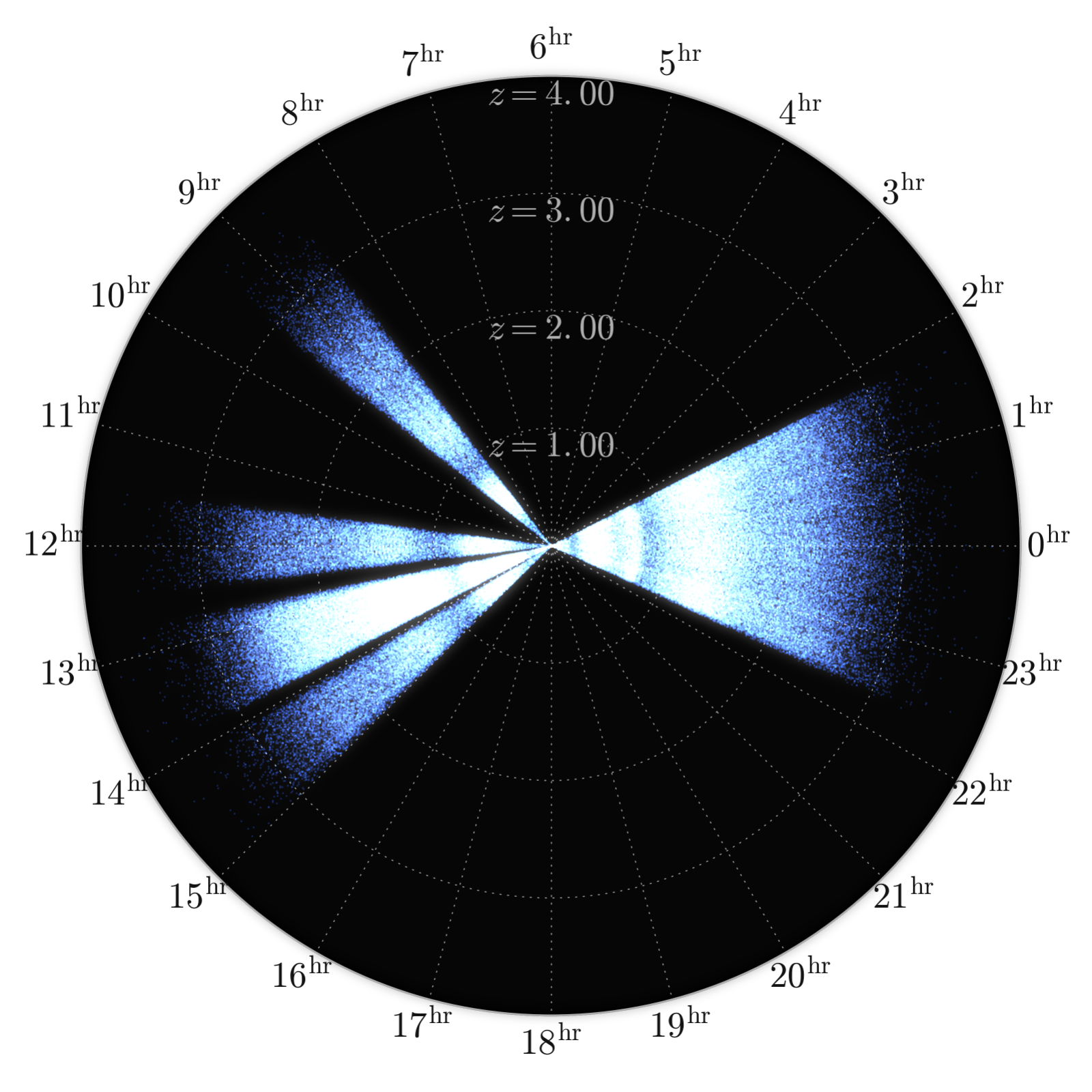
Figure 1: The radial and angular distribution of sub-mm galaxies in all of the five Herschel-ATLAS patches. Note that photometric redshifts have been used to place sources along the redshift axis.

2.4 Galaxy Redshift distribution

The knowledge of the galaxies’ redshifts, along with their uncertainties, plays a fundamental role. One one hand, it enables to construct pixelized maps of the projected galaxy distribution in the respective redshift bins. On the other hand, it allows to predict the theoretical cross-power spectrum that is ultimately compared to the measured one and through that, carry out the cosmological and astrophysical inference.

Following Bianchini et al. (2015, 2016), we estimate the photometric redshift of each source by $\chi^{2}$-fitting the observed Herschel photometric points to a typical high-$z$ SED. Our baseline SED choice is that of SMM J2135-0102, ”The Cosmic Eyelash” at $z=2.3$ (Ivison et al., 2010; Swinbank et al., 2010), that has been shown by Lapi et al. (2011) and González-Nuevo et al. (2012) to be a good template for $z\gtrsim 1$, with a median value of $\Delta z/(1+z)\equiv(z_{\rm ph}-z_{\rm spec})/(1+z_{\rm spec})=-0.002$ and a normalized scatter of $\sigma_{\Delta z/(1+z)}=0.115$. The redshift-dust temperature degeneracy affecting the SED fitting becomes worse at lower redshifts, thus we restrict the analysis to $z_{\rm ph}\geq 1.5$. The robustness of the analysis results with respect to the choice of the assumed SED is tested in Sec. 5.4.

Following Budavari et al. (2003), we model the redshift distribution $p(z|\mathcal{W})$ of galaxies selected by our window function $\mathcal{W}(z_{\rm ph})$ as:

$$p(z|\mathcal{W})=p(z)\int dz_{\rm ph}\mathcal{W}(z_{\rm ph})p(z_{\rm ph}|z),$$ (3)

where $p(z)$ is the fiducial redshift distribution, $\mathcal{W}(z_{\rm ph})$ is 1 for $z_{\rm ph}$ in a selected photo-$z$ interval and 0 otherwise. $p(z_{\rm ph}|z)$ is the probability that a galaxy with a true redshift $z$ has a photometric redshift $z_{\rm ph}$ and is parameterized as a Gaussian distribution with zero mean and scatter $(1+z)\sigma_{\Delta z/(1+z)}$. The resulting redshift distribution is shown in Fig. 2. We normalize $p(z|\mathcal{W})$ to unity and finally calculate the redshift distribution $dN/dz$ as $\frac{dN}{dz}=\left(\int dz^{\prime}p(z^{\prime}|\mathcal{W})\right)^{-1}p(z|\mathcal{W})$. We do not account for the effect of catastrophic redshifts failures in the modelling. In fact, when comparing the photo-$z$ estimated with the SMM or Pearson et al. (2013) template (see Sec. 5.4 for a robustness check using another SED template) to a subset of sources with known spectroscopic redshift, outliers (defined as those objects for which $|\Delta z/(1+z_{\rm spec})|>0.3)$ are much less than 10%, as it can be seen in e.g. Fig. 5 of Ivison et al. (2016). In particular, outliers become more important at redshifts well below $z<0.5$ (see Fig. 6 of Pearson et al. (2013)), but in our analysis we considered only objects with estimated photo-$z$ larger than $z\geq 1.5$ to mitigate this effect as much as possible.

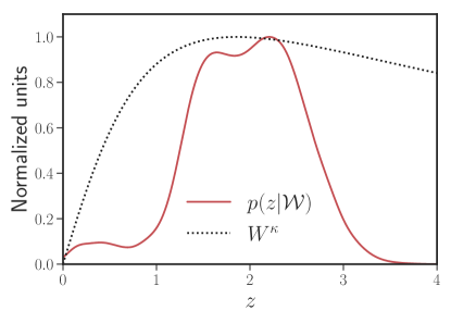
Figure 2: Redshift distribution (solid red line) of the sub-mm sources used in this work allows to probe the peak of the lensing kernel (dotted black line). The CMB lensing kernel $W^{\kappa}$ reflects the relative size of the CMB lensing signal for a fixed mass object at different redshifts; the maximum signal is observed for objects around $1.5\lesssim z\lesssim 2$.

2.5 Galaxy Overdensity Simulations

To generate realizations of the galaxy field comprising of signal and noise with statistical properties that match those of the data, we follow the approach in Smith et al. (2007). We start by generating a simulated galaxy counts map, where the value at each pixel $p$ is spatially modulated by a Gaussian field $g$ generated from the fiducial galaxy auto-spectrum $C_{L}^{gg}$. For each pixel, this is accomplished by drawing a number from a Poissonian distribution with mean $\lambda(p)=\bar{n}(1+g(p))$, where $\bar{n}$ is defined in Sec. 2.3. Finally, we convert the galaxy counts map to overdensity as done for the real galaxies.

3 Theory

The observed CMB lensing and galaxy overdensity fields trace the same underlying matter fluctuations in different and complementary ways. Galaxies are biased signposts of the same dark matter haloes that are lensing the CMB photons. Whereas lensing probes the integrated matter distribution along the line-of sight, galaxy surveys provide a biased sparse sampling of the dark matter field. Both the projected CMB lensing convergence $\kappa(\hat{\mathbf{n}})$ and galaxy overdensity $\delta_{g}(\hat{\mathbf{n}})$ fields along a given line-of-sight $\hat{\mathbf{n}}$ can be expressed as a weighted integral of the 3D dark matter density contrast $\delta$,

$$X(\hat{\mathbf{n}})=\int_{0}^{z_{*}}dz\,W^{X}(z)\delta(\chi(z)\hat{\mathbf{n}},z).$$ (4)

Here $X=\{\kappa,\delta_{g}\}$ and the two fields’ response to the underlying matter distribution is encoded by the kernels $W^{X}(z)$, while $\chi(z)$ denotes the comoving distance to redshift $z$. In the case of CMB lensing convergence, the kernel is given by

$$W^{\kappa}(z)=\frac{3\Omega_{m}}{2c}\frac{H_{0}^{2}}{H(z)}(1+z)\chi(z)\frac{\chi_{*}-\chi(z)}{\chi_{*}},$$ (5)

where $H(z)$ is the Hubble factor at redshift $z$ and $\chi_{*}$ is the comoving distance to the last scattering surface. $\Omega_{m}$ and $H_{0}$ are the present-day values of matter density and Hubble parameter, respectively.

The galaxy overdensity kernel can be written as the sum of two terms, one describing the intrinsic clustering of the sources and one quantifying the so-called magnification bias effect, the apparent clustering of the sources due to the lensing by foreground matter clumps (Turner, 1980; Moessner et al., 1998):

$$W^{\delta_{g}}(z) =b(z)\frac{dN}{dz}+\mu(z),$$ (6)

$$\mu(z) =\frac{3\Omega_{\rm m}}{2c}\frac{H_{0}^{2}}{H(z)}(1+z)\chi(z)$$ (7)

$$\times\int_{z}^{z_{*}}dz^{\prime}\,\left(1-\frac{\chi(z)}{\chi(z^{\prime})}\right)(\alpha(z^{\prime})-1)\frac{dN}{dz^{\prime}}.$$ (8)

In the above equation, we have assumed a linear, local, and deterministic galaxy bias $b(z)$ to relate the galaxy overdensity $\delta_{g}$ to the matter overdensity $\delta$ (Fry & Gaztanaga, 1993), while $dN/dz$ denotes the unit-normalized redshift distribution of the galaxy sample (we use the red solid curve in Fig. 2). Note that the magnification bias term is independent on the galaxy bias parameter but depends, in the weak lensing limit, on the slope $\alpha(z)$ of the integrated galaxy number counts above the flux density limit $S_{\rm min}$ of the survey

$$N(>S_{\rm min})\propto S^{-\alpha}.$$ (9)

For the high-$z$ galaxies selected in this work, Gonzalez-Nuevo et al. (2014); Bianchini et al. (2015) have shown that the magnification bias is substantial. The reason is that the source counts are steep. In fact, the slope of the integrated number counts at the flux limit, as measured from the data at 250 $\mu$m where the main selection is operated, is $\alpha\simeq 3$.

Given that we are interested in sub-degree and degree angular scales ($\ell\gg 10$), we can safely adopt the so-called Limber approximation (Limber, 1953) and evaluate the theoretical cross-power spectrum at a given angular multipole $\ell$ as:

$$C_{\ell}^{\kappa g}=\int_{0}^{z_{*}}\frac{dz}{c}\frac{H(z)}{\chi^{2}(z)}W^{\kappa}(z)W^{\delta_{g}}(z)P_{\rm NL}\left(k=\frac{\ell+\tfrac{1}{2}}{\chi(z)},z\right).$$ (10)

We compute the non-linear matter power spectrum $P_{\rm NL}(k,z)$ using the CAMB code (Lewis et al., 2000) with the Halofit prescription of Takahashi et al. (2012). As can be seen from Eq. 10, the cross-power spectrum $C_{\ell}^{\kappa g}$ is sensitive to the parameter combination $b(z)\sigma_{8}^{2}(z)$, where $\sigma_{8}(z)$ measures the amplitude of the (linear) power spectrum on the scale of 8 $h^{-1}$ Mpc at redshift $z$.

Under the assumption that both the CMB lensing potential and the galaxy overdensity fields behave as Gaussian random fields, we can forecast the expected signal-to-noise ($S/N$). For the survey specifications discussed above, and an assumed galaxy bias $b=3$ (Bianchini et al., 2015; Amvrosiadis et al., 2018), we forecast an overall $S/N$ for $100\leq L\leq 1500$ of 3.4. This is somewhat smaller than the observed value presented in Sec. 5. As we shall see, the reason is that the inferred galaxy bias value is larger than the one assumed for this S/N forecast.

4 Methods

4.1 Power Spectrum Estimation

We measure the cross-correlation signal between CMB lensing and the spatial galaxy distribution in the Fourier domain. As a first step, we perform a real-space convolution between both the CMB lensing $\hat{\kappa}$ and $\hat{\delta}_{g}$ data maps and a tapering function, in order to minimize the noise leakage from large scale to small scales (e.g., Das et al., 2009). Even though the convolution is performed in real-space, we use simulations to evaluate the corresponding transfer function $F_{L}$ that allows us to deconvolve the final cross-power spectrum measurement for its effect following Hivon et al. (2002). The shape of the filter function in the Fourier domain is shown in Fig. 3.

Figure 3: Harmonic counterpart of the real-space filter that we apply to the CMB lensing and galaxy density maps.

After multiplying the convolved maps by the mask, we calculate the Fourier transforms of the observed fields $\hat{\kappa}(\boldsymbol{\ell})$ and $\hat{\delta}_{g}(\boldsymbol{\ell})$, and estimate the 1D cross-power spectrum of the windowed maps in the flat-sky approximation as

$$\hat{C}_{L}^{\kappa g}=f_{\rm sky}^{-1}\left\langle\Re\left[\hat{\kappa}(\boldsymbol{\ell})\hat{\delta}_{g}^{*}(\boldsymbol{\ell})\right]\right\rangle_{\boldsymbol{\ell}\in L},$$ (11)

where $\Re$ denotes the real part of a complex quantity, the average is over all the pixels in the Fourier plane $\boldsymbol{\ell}=(\ell_{x},\ell_{y})$ that fall within the bandpower associated to $L$, and the “ $\hat{}$ ” indicates quantities measured from the data. We account for the effect of masking by rescaling the observed power for $f_{\rm sky}$, the effective area calculated as the mean of the squared mask. Similar to our previous analysis of POLARBEAR Collaboration (2014a), the cross-power spectrum is reconstructed in five multipole bins between $100\leq L\leq 1500$, probing physical scales between 55 Mpc and 4 Mpc at an effective redshift of $\langle z\rangle\sim 2$. We generate 500 correlated CMB lensing and galaxies overdensity simulations that include both the sky signal and noise to check that the power spectrum estimator correctly recovers the input theory within the measured errors without introducing any spurious correlations.

After extracting the power spectra for each lensing quadratic estimator $\alpha=\{EE,EB\}$ and field $f=${RA12,RA23}, we co-add the individual $\hat{C}_{L}^{\kappa g,\alpha,f}$ in a single estimate as

$$\hat{C}_{L}^{\kappa g}=\frac{\sum_{\alpha,f}w_{L}^{\alpha,f}\hat{C}_{L}^{\kappa g,\alpha,f}}{\sum_{\alpha,f}w_{L}^{\alpha,f}},$$ (12)

where the weights $w_{L}^{\alpha,f}$ for the bandpowers of each field and estimator are given by the inverse of the variance of the bandpowers, i.e. the diagonal component of the covariance matrices.

The covariance matrices $\mathbb{C}_{LL^{\prime}}$ are estimated in a Monte Carlo (MC) approach by cross-correlating the observed H-ATLAS density maps with 500 simulated Polarbear lensing convergence maps. We have checked that cross-correlating the true Polarbear CMB lensing convergence maps with simulated galaxy density maps with statistical properties that match that of the data yields comparable error bars.

4.2 Null Tests

We adopt a blind analysis strategy to mitigate observer bias and increase the robustness of our results. Before unblinding the cross-power spectrum, we thus perform a suite of 15 null tests to test for the presence of systematic effects summarized in Table 1. Within this suite, we define two sub-suites: the Polarbear suite and the Analysis suite.

4.2.1 Polarbear Suite

The Polarbear suite definition follows PB17 and consists of 12 different data splits sensitive to multiple sources of instrumental systematic contamination, such as contaminations due to the atmosphere or the telescope sidelobes pickup, systematic effects in the telescope beam or detector response, and vibrations due to the telescope motion. From the two halves of each Polarbear suite data splits we reconstruct two CMB convergence maps and then take the difference between them before computing the null cross-power spectrum with the galaxy density.

4.2.2 Analysis Suite

The Analysis suite consists of a test aimed at assessing the consistency of the source catalog (galaxy catalog null test), and two other tests targeting the robustness of the analysis pipeline, namely the swap-field and the curl null test. In the galaxy catalog null test, we compute the difference of two galaxy overdensity maps of two random halves of the H-ATLAS catalog and correlate it with the Polarbear convergence maps. In the swap-field test, we cross-correlate the Polarbear maps with non-overlapping Herschel galaxy density maps, e.g. Polarbear RA23 with Herschel RA12. Finally, for the curl null test, we reconstruct the curl component of the CMB lensing field (which is expected to be zero at linear order (Fabbian et al., 2018) and without systematic artifacts) and cross-correlate it with the Herschel map on the same sky region.

Table 1: Summary of the null tests performed in this work.

Null test suite	Null test type
Polarbear	Dataset first half vs second half
	First season vs second season
	Focal plane pixel type
	High vs low elevation observations
	Rising vs setting
	High gain vs low gain
	Good vs bad weather
	Moon distance
	Sun distance
	Sun above vs below the horizon
	Left vs right side of the focal plane
	Left vs right-going subscans
Analysis	Galaxy catalog
	Curl mode
	Swap-field

4.2.3 Null Test Statistics

For each null spectrum band power $L$, we calculate the statistic $\chi^{\rm null}_{L}\equiv\hat{C}_{L}^{\rm null}/\sigma_{L}$, where $\sigma_{L}$ is a MC-based estimate of the standard deviation of the null spectra. In our null test framework, we use both $\chi^{\rm null}_{L}$ and $(\chi^{\rm null}_{L})^{2}$ as the former is sensitive to systematic biases while the latter is mostly sensitive to outliers. From these two quantities, we compute four statistics for the minimum-variance cross-power spectrum to test for systematic contamination affecting a particular test or bin: i) average $\chi_{\rm null}$ over all tests and bins; ii) most extreme $\chi^{2}_{\rm null}$ by bin when summing over all null tests; iii) most extreme $\chi^{2}_{\rm null}$ by null test when summing over all bins; iv) total $\chi^{2}_{\rm null}$, summed over all tests and bins. For each of these statistics, we calculate the probability-to-exceed (PTE) by comparing the statistic value found for real data with values found in MC simulations. Additionally, we compute a Kolmogorov-Smirnov (KS) test by comparing the distribution of the $\chi^{2}_{\rm null}$ by test and by bin PTEs to an uniform distribution. In order to consider the null tests passed, we require that the two PTEs of the KS tests and the worst PTEs of the four statistics discussed above are larger than 5% for both the Polarbear and Analysis suites individually and combined. As can be seen in Tab. 2, these requirements are all met. Therefore, we find that systematic effects are well below the statistical detection level.

Table 2: Null test suites summary statistics.

Null test suite	Worst PTE	KS by bin	KS by test
All tests	28%	62%	85%
Polarbear	28%	67%	92%
Analysis	55%	97%	92%

5 Results

5.1 Cross-power Spectrum

The final cross-power spectrum between the Polarbear CMB lensing convergence maps and the H-ATLAS galaxy overdensity is shown in Fig. 4. As mentioned in Sec. 4.1, we calculate the error bars on the band powers by cross-correlating 500 realizations of the CMB lensing field as reconstructed by the Polarbear pipeline with the real H-ATLAS maps. By doing so, the two maps are uncorrelated, which turns out to be a well-founded assumption since $(C_{L}^{\kappa\kappa}+N_{L}^{\kappa\kappa})(C_{L}^{gg}+N_{L}^{gg})\gg(C_{L}^{\kappa g})^{2}$ over the relevant scales. More quantitatively, adopting our fiducial cross-correlation model, we have checked that neglecting the cross-power spectrum term leads to an underestimation of the uncertainties of about 14% for the first bin and less than 5% for the second bandpower. We also note that the covariance matrix is dominated by the diagonal elements, with a neighbouring bins correlation of at most $\approx 15\%$. A statistically significant cross-power is detected. We define the null-hypothesis as the absence of correlation between the CMB lensing and the galaxy fields, i.e. $C_{L}^{\kappa g}=0$. Then, the chi-square value under this null-hypothesis can be evaluated as $\chi^{2}_{\rm null}=\sum_{LL^{\prime}}\hat{C}_{L}^{\kappa g}\mathbb{C}^{-1}_{LL^{\prime}}\hat{C}_{L^{\prime}}^{\kappa g}\simeq 26.1$.

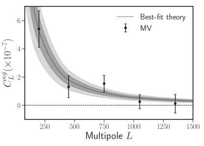
Figure 4: Final cross-power spectrum between Polarbear CMB lensing and the H-ATLAS galaxy overdensity in RA12 and RA23 patches (black circles). The dotted black line represents the best-fit theoretical model (corresponding to a galaxy bias of $b=5.76\pm 1.25$), while the dark and light grey shaded regions indicate the 1 and $2\sigma$ uncertainties respectively.

5.2 Constraints

As we have seen in Sec. 3, the theoretical cross-power spectrum $C_{L}^{\kappa g}$ depends on cosmology, for example through the $\Omega_{m}H_{0}^{2}\sigma_{8}$ combination and astrophysical parameters, such as the galaxy bias $b$. Here, we fix the underlying cosmology and fit for the linear galaxy bias. For reference, the assumed values of matter density, Hubble constant (in km s^-1Mpc^-1), and $\sigma_{8}$ are $\{\Omega_{\rm m},H_{0},\sigma_{8}\}=\{0.3153,67.36,0.8111\}$. The large number of effective independent modes in each band power allows us to assume a Gaussian likelihood as $-2\ln\mathcal{L}(\hat{C}_{L}^{\kappa g}|b)\propto\chi^{2}$, where $\chi^{2}=\sum_{LL^{\prime}}\left[\hat{C}_{L}^{\kappa g}-C_{L}^{\kappa g}(b)\right]\mathbb{C}_{LL^{\prime}}^{-1}\left[\hat{C}_{L^{\prime}}^{\kappa g}-C_{L^{\prime}}^{\kappa g}(b)\right]$. The posterior space is then sampled through a Markov chain Monte Carlo (MCMC) method implemented in the publicly available emcee code (Foreman-Mackey et al., 2013). The resulting best-fit galaxy bias is $b=5.76\pm 1.25$ with a corresponding $\chi^{2}_{\rm bf}\simeq 2.5$ for $\nu=5-1=4$ degrees-of-freedom, or a PTE of about 64%. The significance is computed as the square-root of the difference between the null-line chi-squared value ($b=0$) and the best-fit theory line, $S/N=\sqrt{\chi^{2}_{\rm null}-\chi^{2}_{\rm bf}}\simeq 4.8$.

To give a sense of how an assumption of different cosmological parameters propagates into the inferred constraints on the galaxy bias, we perturb $\sigma_{8}$ by $\pm 3\%$. The corresponding galaxy biases are found to be $b=6.22\pm 1.26$ and $b=5.49\pm 1.12$ (negative and positive perturbations respectively). The differences with respect to the baseline galaxy bias constraint are well within the statistical uncertainty.

The modelling of the magnification bias, encoded by the parameter $\alpha$, also affects the inferred galaxy bias value. To quantify its impact, we have obtained constraints on the galaxy bias assuming two different fiducial values of $\alpha$, namely an unrealistic case where there is no magnification bias ($\alpha=1$) and $\alpha=5$. The respective constraints are $b=9.25^{+1.93}_{-2.04}$ and $b=4.27\pm 0.94$. As expected, by boosting the expected $C_{\ell}^{\kappa g}$, a larger value of $\alpha$ corresponds to a lower galaxy bias.

The galaxy bias constraint can be translated into an estimate of the effective mass $M_{h}$ of the dark matter haloes inhabited by the H-ATLAS galaxies. We assume the bias model provided by Tinker et al. (2010) and relate the scale-independent galaxy bias to the peak height of the linear density field $\nu=\delta_{c}/\sigma(M)$, where $\delta_{c}=1.686$ is the critical threshold for spherical collapse and $\sigma(M)$ is the root mean square density fluctuation for a mass $M$. We infer that, at an effective redshift of $\langle z\rangle\sim 2$, these sub-mm galaxies are hosted by haloes of characteristic mass of $\log_{10}(M_{h}/M_{\odot})=13.5^{+0.2}_{-0.3}$.

From the observational point of view, several authors have studied the clustering properties of galaxies selected at both short (250-500 $\mu$m) and long (850-1200 $\mu$m) sub-mm wavelengths. Numerical simulations have shown that the expected characteristic mass of haloes inhabited by sub-mm sources at $z\sim 2$ is $M_{h}\sim 10^{13}M_{\odot}$ (e.g. Davé et al., 2010; McAlpine et al., 2019). However, a direct comparison between the mass estimates found in different studies is complicated by a number of selection effects that affect the galaxies samples being analyzed. As a result, the inferred halo mass range spans about 1 dex (e.g., Casey et al., 2014; Cowley et al., 2016; Wilkinson et al., 2017). Nonetheless, we attempt to place our measurement in the broader context of similar analyses.

The first thing to notice is that the galaxy bias inferred, or the corresponding effective halo mass, seems to fall in the higher end of the mass spectrum found by previous studies, although the uncertainties are relatively large. For example, Cooray et al. (2010) measured the angular correlation function of Herschel galaxies at $z\sim 2$ with $S_{250\mu m}>30$ mJy and inferred a bias of $2.9\pm 0.4$, corresponding to effective halo masses of $(5\pm 4)\times 10^{12}M_{\odot}$. For sub-mm galaxies between $1\lesssim z\lesssim 3$ detected at 870 $\mu$m with LABOCA, Hickox et al. (2012) have derived a corresponding dark matter halo mass of $\log_{10}(M_{h}/[M_{\odot}h^{-1}])=12.8^{+0.3}_{-0.5}$, consistent with measurements for optically selected quasi-stellar objects. Similarly, clustering measurements of the bright sub-mm galaxies detected by SCUBA-2 at 850 $\mu$m by Wilkinson et al. (2017) suggest that these objects occupy high-mass dark matter halos ($M_{h}>10^{13}M_{\odot}$) at redshifts $z>2.5$. More recently, Amvrosiadis et al. (2018) have measured the angular correlation function of the sub-mm H-ATLAS galaxies with flux densities $S_{250\mu m}>$30 mJy within the NGP and GAMA fields, finding that they typically reside in dark matter haloes of mass $\log_{10}(M_{h}/[M_{\odot}h^{-1}])=13.2\pm 0.1$ across the redshift range $1<z<5$.

Finally, we note that similar information can be extracted from the clustering of CIB fluctuations with the caveat that, differently from catalog-based analysis, diffuse CIB includes emission from unresolved galaxies with fainter far-IR luminosities (hence less massive). For example, Viero et al. (2009) analyzed the CIB anisotropies measured at 250 $\mu$m by BLAST and inferred a bias of $3.8\pm 0.6$ or an effective mass of $\log_{10}(M_{h}/M_{\odot})=12.9\pm 0.3$, while from the angular power spectrum analysis of the CIB fluctuations from Planck, Herschel, SPT and ACT, Xia et al. (2012) found an effective halo mass $\log_{10}(M_{h}/M_{\odot})\sim 12.7$ (no errors given) for sub-mm galaxies at $z\sim 2$.

To further test the consistency of our results, we follow Bianchini et al. (2015); Giannantonio et al. (2016); Omori et al. (2018) and introduce an overall multiplicative bias $A$ that scales the cross-correlation as $\hat{C}_{L}^{\kappa g}=AC_{L}^{\kappa g}(b)$. We can interpret $A$ as the lensing amplitude, and a value of $A$ different from unity can be ascribed to the presence of systematics, to improper modelling of the signal, to a mismatch in the assumed underlying cosmology, and possibly to new physics. Of course there will be a degeneracy between the amplitude $A$ and the galaxy bias, since the cross-power spectrum probes a combination of $bA$. In fact, the aforementioned studies combine the cross-correlation and the galaxy clustering measurements, that scales as $b^{2}$ albeit at the price of being more prone to systematics, to break such degeneracies. Nonetheless, we adopt the same MCMC approach outlined above and infer a constraint on $bA=5.69\pm 1.30$. In light of the above discussion on the bias constraints from literature, one would expect a $bA$ value around 3 $\sim$ 4. This value is approximately 1.5 $\sim 2\sigma$ lower than we measured.

When examining the cross-spectrum of the two fields separately, we find that the high value is coming from the RA12 field. A plausible explanation for the high value of the bias is that the lensing signal in this small ($\sim$ 5 $\deg^{2}$) field has scattered high due to sample variance. The Polarbear lensing map is sample variance limited in the first two multipole bins, which drive the amplitude constraint. A precise estimate of the significance of the observed scatter in the RA12 cross-spectrum is not straightforward to quantify without, for example, the knowledge of the exact galaxy bias value. Given that the power excess is driven by the first band power around $L\sim 200$, we have performed the following check in order to understand whether the scatter is anomalous or not. We have extracted the CMB lensing-galaxy density cross-spectrum $C_{L}^{\kappa g}$ between a set of correlated (Gaussian) lensing and galaxy realizations and measured the ratio between the first band power value and the statistical uncertainties, $C_{L}^{\kappa g}/\Delta C_{L}^{\kappa g}$. We found that, in about 4% of the simulations, the first band power lies more 4$\sigma$ (the value found in data) away from the null line. We then conclude that, although large, this fluctuation does not seem to be anomalous. Finally, we note that an excess of power is also observed in RA12 in cross-correlation with galaxy lensing from the Hyper Suprime-Cam (Namikawa et al., 2019) even though with larger error bars. We also stress that this pipeline used a completely independent lensing reconstruction pipeline.

5.3 Comparison with Planck

Our result can be directly compared to the one of Bianchini et al. (2016). In that paper, the authors correlated the same H-ATLAS sources catalog adopted here with the publicly available all-sky CMB lensing convergence map from Planck (Planck Collaboration, 2016a). Specifically, the authors exploited the full overlap between the H-ATLAS survey and the Planck footprint to reconstruct the cross-power spectrum $C_{L}^{\kappa g}$ between $100\leq L\leq 800$.

As it can be seen in Fig. 5, the amplitude and shape of cross-spectrum is similar to the one measured with Polarbear maps over the range of scales where the visual comparison can be performed. It is also interesting to note that, despite the sky coverage being almost 30 times smaller than that of the Planck $\times$ H-ATLAS analysis, we still detect a signal only $\sim 4$ times less significant thanks to the high sensitivity of the Polarbear CMB lensing convergence maps.

The linear galaxy bias inferred by fitting the Planck $\times$ H-ATLAS cross-power spectrum $\hat{C}_{L}^{\kappa g}$ to the theoretical model is $b=3.43\pm 0.51$, roughly $2\sigma$ away from the central value found in our analysis. This corresponds to an effective host halo mass of about $\log_{10}(M_{h}/M_{\odot})=12.9^{+0.2}_{-0.2}$. When including the amplitude $A$, the MCMC analysis reveals a constraint of $bA=3.40\pm 0.51$.

We also stress that our measurement fundamentally differs from the one based on Planck data. While Polarbear lensing convergence maps have been obtained from polarization data only, where the strength of both thermal Sunyaev-Zel’dovich (tSZ) and CIB emissions is greatly reduced because they both are essentially unpolarized, the Planck CMB lensing map is dominated by the information provided by CMB temperature (even though the released map is a minimum variance one and includes also polarization data). In principle, residuals of extragalactic foreground emission such as tSZ effect in galaxy clusters or the CIB emission could contaminate the Planck CMB lensing map. Because these emissions are correlated between themselves and with the distribution of the LSS (Planck Collaboration, 2016b), they could affect the amplitude of the cross-correlation as positive biases. In particular, the H-ATLAS galaxies have fluxes well below the Planck detection limits and contribute, at least partially, to any residual CIB emission present in the Planck maps. However, semi-analytic estimates indicate that possible induced biases on the temperature reconstruction should not be large at Planck sensitivity level (Osborne et al., 2014; van Engelen et al., 2014) and systematic checks performed by the Planck team found no evidence for such contamination (Planck Collaboration, 2018b). Given the differences that characterize the Polarbear and Planck lensing reconstructions, and since the recovered cross-power spectra shown in Fig. 5 are in good agreement, it is unlikely that foregrounds represent a major source of contamination in our results.

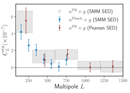
Figure 5: Our baseline measurement of the CMB lensing-galaxy cross-power spectrum over a sky fraction $f_{\rm sky}\approx 3\times 10^{-4}$ (using the SMM template, shown as grey boxes) is in agreement with the $C_{L}^{\kappa g}$ found adopting a different SED template (Pearson et al. (2013) SED, red circles) and with the one based on Planck CMB lensing data over $f_{\rm sky}\approx 0.01$ (band powers from Bianchini et al. (2016), blue squares).

5.4 Effect of the SED Template

Another aspect worth investigating is the effect of the fiducial SED template on the recovered cross-power spectrum. Since the SED plays a crucial role when inferring the photo-$z$s from H-ATLAS photometry, it is important to test the robustness of the results against variations in the assumed SED. To this end, we start from the same galaxy catalog introduced in Sec. 2.3 and estimate the redshift of each source by fitting the SED template from Pearson et al. (2013). This template consists in a two-temperature modified blackbody synthesized from the Herschel PACS and SPIRE flux densities of 40 bright H-ATLAS sources with known spectroscopic redshift (25 of these sources lie at $0.5<z<1$ and have optical spec-$z$s while the remaining 15 sources at $z>1$ have CO spec-$z$s). The uncertainty in the template is $\Delta z/(1+z)\equiv(z_{\rm ph}-z_{\rm spec})/(1+z_{\rm spec})=0.03$ with an r.m.s. of $\sigma_{\Delta z/(1+z)}=0.26$. Using the new redshifts, we find that 5,022 and 7,772 galaxies fall within the RA12 and RA23 patches respectively. We re-run the full analysis pipeline with the galaxy overdensity maps constructed from this catalog and extract the cross-power spectrum shown in Fig. 5 as red circles. As can be seen, in this case too we detect a statistically significant signal, rejecting the null hypothesis with a significance of about $\sqrt{\Delta\chi^{2}}\simeq 4.3$, as opposed to 4.8 in the SMM J2135-0102 case. From a visual inspection, the cross-spectrum appears consistent with what found in the baseline case, with all the shifts well within the $1\sigma$ uncertainties. Band powers errors appear to be slightly larger because of the reduced number of galaxies at $z\geq 1.5$, hence a larger shot-noise. A possible explanation is that the inclusion of sources with optical spec-$z$ at $z<1$ in the calibration of the Pearson et al. (2013) template resulted in a redder SED than the average for those sub-mm sources with CO spec-$z$s, which translates into a slight bias towards low-$z$. The galaxy bias analysis reveals a constraint of $b=5.38\pm 1.40$ when using the Pearson et al. (2013) SED as opposed to $b=5.76\pm 1.25$ for our baseline case, meaning that the systematic shift $\Delta b\approx 0.39$ is smaller than the statistical uncertainties.

5.5 H-ATLAS Galaxies Auto-spectrum

An informative check to perform is recovering the H-ATLAS galaxies auto-power spectrum in the two fields overlapping with Polarbear. Performing a thorough analysis of the galaxy auto-power spectrum would require an extensive validation of the measurement that is beyond the scope of the present work, here we naively recover the galaxy auto-spectrum in the RA12 and RA23 fields. An auto-power spectrum analysis of the H-ATLAS galaxies selected with similar criteria as the ones adopted here can be found in Bianchini et al. (2016). Instead of debiasing the raw galaxy auto-spectra for the shot-noise, we rely on a jackknifing approach. We first randomly split the galaxy catalog in two and create two galaxy overdensity maps, $\delta_{g}^{(1)}$ and $\delta_{g}^{(2)}$. From these, we form a pair of half-sum and half-difference maps, $\delta_{g}^{\pm}=(\delta_{g}^{(1)}\pm\delta_{g}^{(2)})/2$. The former map will contain both signal and noise, while the latter will be noise-only. Then we extract their auto-power spectra and evaluate the total galaxy auto-power spectrum as the difference of the half-sum and half-difference overdensity map, $\hat{C}_{\ell}^{gg}=\hat{C}^{+}_{\ell}-\hat{C}^{-}_{\ell}$. The resulting galaxy auto-spectra in RA12 and RA23 are shown as the red and blue points in Fig. 6. The error bars in the galaxy auto-power spectrum shown in the plot are estimated in the Gaussian approximation using the measured auto-spectra. For comparison, we also include the auto-power spectrum (over the full H-ATLAS fields that cover about 600 deg²) presented in Bianchini et al. (2016). Even though the uncertainties on the individual RA12 and RA23 fields are large, the power observed in RA23 seems comparable to the full H-ATLAS one, while an excess of clustering seems to be present in RA12.

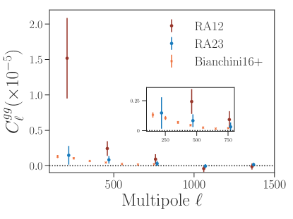
Figure 6: A comparison between the H-ATLAS galaxies auto-power spectrum in the RA12 and RA23 fields (red and blue circles respectively), and the band powers obtained from the full 600 deg² of the H-ATLAS survey by Bianchini et al. (2016) (blue squares).

6 Conclusions

In this paper, we have measured the cross-correlation signal between the CMB lensing convergence maps reconstructed from Polarbear polarization maps and the spatial distribution of the high-$z$ sub-mm galaxies detected by the Herschel satellite. Despite the small size of the overlapping patches, the depth of Polarbear maps together with the redshift extent of the H-ATLAS sources optimally matched to the CMB lensing kernel, have enabled the detection of the cross-power spectrum at a significance of 4.8 $\sigma$. This measurement probes large-scale structure at an effective redshift $z\sim 2$.

The cross-correlation power depends on the product $bA$, with a preferred value of $bA=5.69\pm 1.30$. While this is approximately 2 $\sigma$ above the expected value of $3\sim 4$, we hesitate to interpret this as a tension given the limited statistical evidence. The high value is plausibly explained by lensing sample variance over the $\sim$10 $\deg^{2}$ of sky.

We use the galaxy bias information to infer the effective mass of the haloes hosting the H-ATLAS sub-mm sources at a redshift of $z\sim 2$, finding $\log_{10}(M_{h}/M_{\odot})=13.5^{+0.2}_{-0.3}$. This value falls at the high end of the mass spectrum found by previous studies (e.g. Amvrosiadis et al., 2018).

A suite of null tests has been performed to demonstrate that the instrumental systematics are below the statistical detection level. In particular, we stress that lensing reconstructions based on CMB polarization maps, like the one presented in this paper, are less contaminated by galactic and extragalactic foregrounds, providing a clearer view of the projected matter distribution along the line-of-sight. Furthermore, the robustness of the results is corroborated by the good agreement between our cross-correlation power measurement and the one based on Planck CMB lensing (Bianchini et al., 2016).

Cross-correlations between CMB lensing and LSS tracers, and multi-pronged approaches in general, are becoming a standard tool in cosmological analysis. In the upcoming years, with the advent of new generation experiments such as the Simons Array (Suzuki et al., 2016) and the Simons Observatory (The Simons Observatory Collaboration, 2019) that will have similar depths over much larger areas of the sky, the full potential of cross-correlation measurements will be unleashed and provide deeper insights on cosmological issues, such as the nature of dark matter, dark energy, and neutrinos, as well as on galaxy formation and evolution.

References

- Abbott et al. (2018) Abbott, T. M. C., Abdalla, F. B., Alarcon, A., et al. 2018, arXiv e-prints, arXiv:1810.02322
- Aghanim et al. (2008) Aghanim, N., Majumdar, S., & Silk, J. 2008, Reports on Progress in Physics, 71, 066902
- Allison et al. (2015) Allison, R., Lindsay, S. N., Sherwin, B. D., et al. 2015, Monthly Notices of the Royal Astronomical Society, 451, 849
- Amvrosiadis et al. (2018) Amvrosiadis, A., Valiante, E., Gonzalez-Nuevo, J., et al. 2018, MNRAS, 2881
- Arnold et al. (2012) Arnold, K., Ade, P. A. R., Anthony, A. E., et al. 2012, in Society of Photo-Optical Instrumentation Engineers (SPIE) Conference Series, Vol. 8452, Millimeter, Submillimeter, and Far-Infrared Detectors and Instrumentation for Astronomy VI, 84521D
- Baxter et al. (2016) Baxter, E. J., Clampitt, J., Giannantonio, T., et al. 2016, eprint arXiv, 1602, arXiv:1602.07384
- Beck et al. (2018) Beck, D., Fabbian, G., & Errard, J. 2018, Phys. Rev. D, 98, 043512
- Bianchini & Reichardt (2018) Bianchini, F., & Reichardt, C. L. 2018, Astrophys. J., 862, 81
- Bianchini et al. (2015) Bianchini, F., Bielewicz, P., Lapi, A., et al. 2015, ApJ, 802, 64
- Bianchini et al. (2016) Bianchini, F., et al. 2016, Astrophys. J., 825, 24
- BICEP2/Keck Array Collaboration (2016) BICEP2/Keck Array Collaboration. 2016, ApJ, 833, 228
- Blain et al. (2002) Blain, A. W., Smail, I., Ivison, R. J., Kneib, J. P., & Frayer, D. T. 2002, Phys. Rep., 369, 111
- Bleem et al. (2012) Bleem, L. E., van Engelen, A., Holder, G. P., et al. 2012, The Astrophysical Journal, 753, L9
- Böhm et al. (2016) Böhm, V., Schmittfull, M., & Sherwin, B. D. 2016, Phys. Rev. D, 94, 043519
- Böhm et al. (2018) Böhm, V., Sherwin, B. D., Liu, J., et al. 2018, Phys. Rev., D98, 123510
- Bourne et al. (2016) Bourne, N., Dunne, L., Maddox, S. J., et al. 2016, MNRAS, 462, 1714
- Budavari et al. (2003) Budavari, T., Connolly, A. J., Szalay, A. S., et al. 2003, The Astrophysical Journal, 595, 59
- Casey et al. (2014) Casey, C. M., Narayanan, D., & Cooray, A. 2014, Phys. Rep., 541, 45
- Challinor et al. (2018) Challinor, A., et al. 2018, JCAP, 1804, 018
- Cooray et al. (2010) Cooray, A., Amblard, A., Wang, L., et al. 2010, A&A, 518, L22
- Cowley et al. (2016) Cowley, W. I., Lacey, C. G., Baugh, C. M., & Cole, S. 2016, MNRAS, 461, 1621
- Das et al. (2009) Das, S., Hajian, A., & Spergel, D. N. 2009, Phys. Rev. D, 79, 083008
- Das et al. (2014) Das, S., Louis, T., Nolta, M. R., et al. 2014, Journal of Cosmology and Astro-Particle Physics, 2014, 014
- Davé et al. (2010) Davé, R., Finlator, K., Oppenheimer, B. D., et al. 2010, MNRAS, 404, 1355
- DiPompeo et al. (2014) DiPompeo, M. A., Myers, A. D., Hickox, R. C., et al. 2014, Monthly Notices of the Royal Astronomical Society, 446, 3492
- Dunne et al. (2011) Dunne, L., Gomez, H. L., da Cunha, E., et al. 2011, Monthly Notices of the Royal Astronomical Society, 417, 1510
- Eales et al. (2010) Eales, S., Dunne, L., Clements, D., et al. 2010, Publications of the Astronomical Society of the Pacific, 122, 499
- Eales et al. (2018) Eales, S., Smith, D., Bourne, N., et al. 2018, MNRAS, 473, 3507
- Fabbian et al. (2018) Fabbian, G., Calabrese, M., & Carbone, C. 2018, Journal of Cosmology and Astro-Particle Physics, 2018, 050
- Fabbian & Stompor (2013) Fabbian, G., & Stompor, R. 2013, A&A, 556, A109
- Foreman-Mackey et al. (2013) Foreman-Mackey, D., Hogg, D. W., Lang, D., & Goodman, J. 2013, PASP, 125, 306
- Fry & Gaztanaga (1993) Fry, J. N., & Gaztanaga, E. 1993, ApJ, 413, 447
- Giannantonio & Percival (2014) Giannantonio, T., & Percival, W. J. 2014, Monthly Notices of the Royal Astronomical Society: Letters, 441, L16
- Giannantonio et al. (2016) Giannantonio, T., Fosalba, P., Cawthon, R., et al. 2016, MNRAS, 456, 3213
- González-Nuevo et al. (2012) González-Nuevo, J., Lapi, A., Fleuren, S., et al. 2012, The Astrophysical Journal, 749, 65
- Gonzalez-Nuevo et al. (2014) Gonzalez-Nuevo, J., Lapi, A., Negrello, M., et al. 2014, Monthly Notices of the Royal Astronomical Society, 442, 2680
- Griffin et al. (2010) Griffin, M. J., Abergel, A., Abreu, A., et al. 2010, Astronomy and Astrophysics, 518, L3
- Guo et al. (2011) Guo, Q., Cole, S., Lacey, C. G., et al. 2011, Monthly Notices of the Royal Astronomical Society, 412, 2277
- Hickox et al. (2012) Hickox, R. C., Wardlow, J. L., Smail, I., et al. 2012, MNRAS, 421, 284
- Hirata et al. (2008) Hirata, C. M., Ho, S., Padmanabhan, N., Seljak, U., & Bahcall, N. A. 2008, Physical Review D - Particles, Fields, Gravitation and Cosmology, 78, arXiv:0801.0644
- Hirata & Seljak (2003) Hirata, C. M., & Seljak, U. 2003, Physical Review D, 67, arXiv:0209489
- Hivon et al. (2002) Hivon, E., Górski, K. M., Netterfield, C. B., et al. 2002, ApJ, 567, 2
- Holder et al. (2013) Holder, G. P., Viero, M. P., Zahn, O., et al. 2013, The Astrophysical Journal, 771, L16
- Hu & Okamoto (2002) Hu, W., & Okamoto, T. 2002, ApJ, 574, 566
- Hunter (2007) Hunter, J. D. 2007, Computing In Science & Engineering, 9, 90
- Ivison et al. (2010) Ivison, R. J., Swinbank, A. M., Swinyard, B., et al. 2010, Astronomy and Astrophysics, 518, L35
- Ivison et al. (2016) Ivison, R. J., Lewis, A. J. R., Weiss, A., et al. 2016, The Astrophysical Journal, 832, 78
- Jones et al. (2001–) Jones, E., Oliphant, T., Peterson, P., et al. 2001–, SciPy: Open source scientific tools for Python, , , [Online; accessed ¡today¿]
- Kermish et al. (2012) Kermish, Z. D., Ade, P., Anthony, A., et al. 2012, in Society of Photo-Optical Instrumentation Engineers (SPIE) Conference Series, Vol. 8452, Millimeter, Submillimeter, and Far-Infrared Detectors and Instrumentation for Astronomy VI, 84521C
- Kuo et al. (2007) Kuo, C. L., Ade, P. A. R., Bock, J. J., et al. 2007, ApJ, 664, 687
- Lapi et al. (2011) Lapi, A., González-Nuevo, J., Fan, L., et al. 2011, The Astrophysical Journal, 742, 24
- Lewis (2005) Lewis, A. 2005, Phys. Rev. D, 71, 083008
- Lewis & Challinor (2006) Lewis, A., & Challinor, A. 2006, Weak gravitational lensing of the CMB, , , arXiv:0601594
- Lewis et al. (2000) Lewis, A., Challinor, A., & Lasenby, A. 2000, ApJ, 538, 473
- Limber (1953) Limber, D. N. 1953, ApJ, 117, 134
- Maddox et al. (2010) Maddox, S. J., Dunne, L., Rigby, E., et al. 2010, Astronomy and Astrophysics, 518, L11
- Maddox et al. (2018) Maddox, S. J., Valiante, E., Cigan, P., et al. 2018, ApJS, 236, 30
- McAlpine et al. (2019) McAlpine, S., Smail, I., Bower, R. G., et al. 2019, arXiv e-prints, arXiv:1901.05467
- Moessner et al. (1998) Moessner, R., Jain, B., & Villumsen, J. V. 1998, MNRAS, 294, 291
- Namikawa et al. (2019) Namikawa, T., Chinone, Y., Miyatake, H., et al. 2019, arXiv e-prints, arXiv:1904.02116
- Omori et al. (2017) Omori, Y., Chown, R., Simard, G., et al. 2017, ApJ, 849, 124
- Omori et al. (2018) Omori, Y., et al. 2018, arXiv:1810.02342
- Osborne et al. (2014) Osborne, S. J., Hanson, D., & Doré, O. 2014, J. Cosmology Astropart. Phys, 2014, 024
- Peacock & Bilicki (2018) Peacock, J. A., & Bilicki, M. 2018, Mon. Not. Roy. Astron. Soc., 481, 1133
- Pearson et al. (2013) Pearson, E. A., Eales, S., Dunne, L., et al. 2013, Monthly Notices of the Royal Astronomical Society, 435, 2753
- Pérez & Granger (2007) Pérez, F., & Granger, B. E. 2007, Computing in Science and Engineering, 9, 21
- Pilbratt et al. (2010) Pilbratt, G. L., Riedinger, J. R., Passvogel, T., et al. 2010, Astronomy and Astrophysics, 518, L1
- Planck Collaboration (2014a) Planck Collaboration. 2014a, A&A, 571, A17
- Planck Collaboration (2014b) —. 2014b, A&A, 571, A18
- Planck Collaboration (2016a) —. 2016a, A&A, 10
- Planck Collaboration (2016b) —. 2016b, A&A, 594, A23
- Planck Collaboration (2018a) —. 2018a, arXiv e-prints, arXiv:1807.06209
- Planck Collaboration (2018b) —. 2018b, arXiv e-prints, arXiv:1807.06210
- Poglitsch et al. (2010) Poglitsch, A., Waelkens, C., Geis, N., et al. 2010, Astronomy and Astrophysics, 518, L2
- POLARBEAR Collaboration (2014a) POLARBEAR Collaboration. 2014a, Phys. Rev. Lett., 112, 131302
- POLARBEAR Collaboration (2014b) —. 2014b, Phys. Rev. Lett., 113, 021301
- POLARBEAR Collaboration (2017) —. 2017, ApJ, 848, 121
- POLARBEAR Collaboration (2019) —. 2019, in prep
- Pratten & Lewis (2016) Pratten, G., & Lewis, A. 2016, Journal of Cosmology and Astro-Particle Physics, 2016, 047
- Pullen et al. (2016) Pullen, A. R., Alam, S., He, S., & Ho, S. 2016, MNRAS, 460, 4098
- Sherwin et al. (2012) Sherwin, B. D., Das, S., Hajian, A., et al. 2012, Physical Review D - Particles, Fields, Gravitation and Cosmology, 86, 1
- Sherwin et al. (2017) Sherwin, B. D., van Engelen, A., Sehgal, N., et al. 2017, Phys. Rev. D, 95, 123529
- Smail et al. (1997) Smail, I., Ivison, R. J., & Blain, A. W. 1997, ApJ, 490, L5
- Smith et al. (2007) Smith, K. M., Zahn, O., & Doré, O. 2007, Physical Review D, 76, 043510
- Smith et al. (2009) Smith, K. M., et al. 2009, AIP Conf. Proc., 1141, 121
- Smith et al. (2017) Smith, M. W. L., Ibar, E., Maddox, S. J., et al. 2017, ApJS, 233, 26
- Smith et al. (2003) Smith, R. E., Peacock, J. A., Jenkins, A., et al. 2003, MNRAS, 341, 1311
- Song et al. (2003) Song, Y.-S., Cooray, A., Knox, L., & Zaldarriaga, M. 2003, The Astrophysical Journal, 590, 664
- Stompor & Efstathiou (1999) Stompor, R., & Efstathiou, G. 1999, Monthly Notices of the Royal Astronomical Society, 302, 735
- Story et al. (2015) Story, K. T., Hanson, D., Ade, P. A. R., et al. 2015, ApJ, 810, 50
- Suzuki et al. (2016) Suzuki, A., Ade, P., Akiba, Y., et al. 2016, Journal of Low Temperature Physics, 184, 805
- Swinbank et al. (2010) Swinbank, A. M., Smail, I., Longmore, S., et al. 2010, Nature, 464, 733
- Takahashi et al. (2012) Takahashi, R., Sato, M., Nishimichi, T., Taruya, A., & Oguri, M. 2012, ApJ, 761, 152
- The Simons Observatory Collaboration (2019) The Simons Observatory Collaboration. 2019, Journal of Cosmology and Astro-Particle Physics, 2019, 056
- Tinker et al. (2010) Tinker, J. L., Robertson, B. E., Kravtsov, A. V., et al. 2010, ApJ, 724, 878
- Turner (1980) Turner, E. L. 1980, ApJ, 242, L135
- Valiante et al. (2016) Valiante, E., Smith, M. W. L., Eales, S., et al. 2016, MNRAS, 462, 3146
- van Engelen et al. (2014) van Engelen, A., Bhattacharya, S., Sehgal, N., et al. 2014, ApJ, 786, 13
- van Engelen et al. (2015) van Engelen, A., Sherwin, B. D., Sehgal, N., et al. 2015, The Astrophysical Journal, 808, 7
- Viero et al. (2009) Viero, M. P., Ade, P. A. R., Bock, J. J., et al. 2009, ApJ, 707, 1766
- Wilkinson et al. (2017) Wilkinson, A., et al. 2017, MNRAS, 464, 1380
- Xia et al. (2012) Xia, J. Q., Negrello, M., Lapi, A., et al. 2012, Monthly Notices of the Royal Astronomical Society, 422, 1324
- Zavala et al. (2018) Zavala, J. A., Montaña, A., Hughes, D. H., et al. 2018, Nature Astronomy, 2, 56