Control-Lyapunov and Control-Barrier Functions based Quadratic Program for Spatio-temporal Specifications
Abstract
This paper presents a method for control synthesis under spatio-temporal constraints. First, we consider the problem of reaching a set in a user-defined or prescribed time . We define a new class of control Lyapunov functions, called prescribed-time control Lyapunov functions (PT CLF), and present sufficient conditions on the existence of a controller for this problem in terms of PT CLF. Then, we formulate a quadratic program (QP) to compute a control input that satisfies these sufficient conditions. Next, we consider control synthesis under spatio-temporal objectives given as: the closed-loop trajectories remain in a given set at all times; and, remain in a specific set during the time interval for ; and, reach the set on or before . We show that such spatio-temporal specifications can be translated into temporal logic formulas. We present sufficient conditions on the existence of a control input in terms of PT CLF and control barrier functions. Then, we present a QP to compute the control input efficiently, and show its feasibility under the assumptions of existence of a PT CLF. To the best of authors’ knowledge, this is the first paper proposing a QP based method for the aforementioned problem of satisfying spatio-temporal specifications for nonlinear control-affine dynamics with input constraints. We also discuss the limitations of the proposed methods and directions of future work to overcome these limitations. We present numerical examples to corroborate our proposed methods.
I Introduction
Driving the state of a dynamical system to a given desired set is an important problem, particularly in the fields of robot motion planning and safety-critical control. Various approaches have been developed in past to accomplish this task. Model predictive control (MPC)-based methods [1, 2], rapidly-exploring random tree (RRT) based methods [3, 4, 5], and combinations of them [3] have been studied extensively in the literature. In addition, Lyapunov-based methods, such as vector fields [6, 7] and control Lyapunov functions (CLF) [8, 9, 10] are also popular, in part because these methods are inherently amenable to Lyapunov-based analysis. Control design for systems with input and state constraints is not a trivial task, as these constraints impose limitations on several aspects of the control synthesis. For example, spatial constraints requiring the system trajectories to be in some safe set at all times are common in safety-critical applications. Furthermore, temporal constraints pertaining to convergence within a prescribed time appear in time-critical applications where completion of a task is required within a given time interval. Spatio-temporal specifications impose spatial as well as temporal or time constraints on the system trajectories.
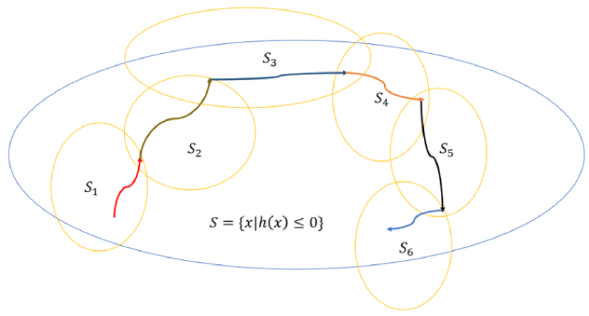
From practical point of view, considering safety constraints, e.g., avoiding collisions in multi-robot systems, avoiding static and dynamic obstacles, and in general, avoiding the unsafe regions in the state space, is crucial. One of the most common methods of incorporating such spatial constraints on the system states is based on control barrier functions (CBF) [11]. Barrier functions are used for the synthesis of safe controllers [11, 12] and barrier certificates are used as a verification tool to guarantee that the closed-loop trajectories remain safe at all times. The authors in [13] present sufficient conditions in terms of existence of a barrier certificate for forward-invariance of a given set, and propose a sum-of-squares formulation to find a Barrier certificate. In order to guarantee safety and convergence, a combination of CLFs and CBFs is used for control design [11, 14, 15]. In the CLF-CBF based controller, convergence is guaranteed due to the CLF and safety is guaranteed due to CBF. [16] utilizes Lyapunov-like barrier functions to guarantee asymptotic tracking of a time-varying output trajectory, while the system output always remains inside a given set. The authors in [11, 14] present conditions using zeroing barrier functions so that the set defined as , where is a user-defined smooth function, is forward invariant.
More recently, quadratic program (QP) based approaches have gained popularity for control synthesis; with this approach, the CLF and CBF conditions are formulated as inequalities that are linear in the control input [8, 9, 11, 17]. These methods are suitable for real-time implementation as QPs can be solved very efficiently. The authors in [11] combine the control performance objectives and safety objectives, represented using CLF and CBF, respectively, via a single QP. Authors in [18] use CBF to encode signal-temporal logic (STL) based specifications and formulate a QP to compute the control input (see [18] for details on STL-based specifications for robot motion planning). The aforementioned work [6, 7], [10]-[17] concerns with designing control laws so that the reachability objectives, such as reaching a desired location or a desired goal set, are achieved as time goes to infinity, i.e., asymptotically.
In contrast to asymptotic stability (AS), which pertains to convergence as time goes to infinity, finite-time stability (FTS) is a concept that guarantees convergence of solutions in finite time. In the seminal work [19], the authors introduce the necessary and sufficient conditions in terms of Lyapunov functions under which continuous, autonomous systems exhibit FTS. The authors in [8] formulate a QP to ensure finite-time convergence of the closed-loop trajectories to a set with input constraints. Fixed-time stability (FxTS) [20] is a stronger notion than FTS, where the time of convergence does not depend upon the initial conditions. More recently, the authors in [21] used the notion or prescribed-time or user-defined time stability, where the time of convergence can be chosen by the user a priori.
In most of the aforementioned work, only one safety and one convergence objectives are considered. In this paper, we consider a multi-task problem of designing a control input. The considered objectives are of the following form: (i) the system trajectories should stay in a given set at all times, (ii) the system trajectories should stay in a set in the time-interval for , where is a user-defined time sequence, (iii) the trajectories should reach the set before time instant , and (iv) the control input should satisfy control constraints at all times. We show that such spatio-temporal specifications can be translated into a STL formula. In [18], the authors consider the problem of generating controller to satisfy STL specifications under the assumption that the system dynamics are equivalent to a single-integrator dynamics. To the best of authors’ knowledge, this is the first paper proposing a QP based method for the aforementioned problem of satisfying spatio-temporal specifications without making any assumptions on the system dynamics. We first study the problem of reaching a given set in a user-defined time for a general class of control-affine systems with input constraints. We extend the proposed formulation to guarantee that once the trajectories reach the desired set , they stay in the set for all future times. We define the new notion of prescribed-time CLF (PT CLF), and use it to solve the problem of reaching a given goal set within a given prescribed time . Then, we present sufficient conditions in terms PT CLF and CBF to guarantee that the given spatio-temporal specifications are met. Finally, we present a QP-based optimization problem that can compute a control input for the same, and show its feasibility under some mild conditions. In contrast to earlier work [8, 9, 11, 18], our proposed framework is able to accommodate spatio-temporal, i.e., both state and time, constraints in the presence of control input constraints. Furthermore, in contrast to the results in [8, 22], where under the traditional notion of FTS, as defined in [19], the convergence time depends upon the initial conditions, the closed-loop system trajectories resulting from our controller reach the given set in a prescribed time that can be chosen arbitrarily and independently of the initial conditions.
The rest of the paper is organized as follows: In Section II, we present the notations used in the paper and background material on various notions of finite-time stability. In Section III, we study the problem of reaching a set in a prescribed time and staying there for all future times. In Section IV, we consider the general multi-task problem for spatio-temporal specifications and formulate a QP to find the control input. We show three numerical examples in Section V to corroborate our theoretical results. We discuss the limitations of the proposed methods and propose a direction to relax the assumptions used in deriving the main results and summarize our thoughts on future work in Section VI. Finally, we present the conclusions in Section VII.
II Mathematical Preliminaries
II-A Notation
denotes the set of reals and denotes the set of non-negative reals. The boundary of a closed set is denoted by and its interior by . The Lie derivative of a function along a vector field is denoted as . We use to denote the -norm of the vector and simply use to denote the Euclidean norm.
II-B Preliminaries
Consider the system:
| (1) |
where and is continuous with . As defined in [19], the origin is said to be an FTS equilibrium of (1) if it is Lyapunov stable and finite-time convergent, i.e., for all , where is some open neighborhood of the origin, , where , depends upon the initial condition . The authors in [20] presented the following result for FxTS, where the time of convergence does not depend upon the initial condition.
Theorem 1 ([20]).
If the settling-time can be chosen a priori by the user, then the origin is called as user-defined or prescribed-time stable [21].
III Prescribed-time Set Reachability
In this section, we consider the problem of reaching a set in a user-defined or prescribed time , where is a user-defined function. Consider the system
| (4) |
where is the state-vector, , are system vector fields, and is the control input. The problem statement can be formally written as:
Problem 1.
Design a control input , so that the closed-loop trajectories of (4) reach the set in a prescribed time , where is a user-defined continuously differentiable function, and are user-defined matrices.
Input constraints of the form are very commonly considered in the literature [11]. Now, we present sufficient conditions for existence of a control input that solves Problem 1. First, we define a new class of CLF with prescribed-time convergence guarantees:
Definition 1.
PT CLF-: A continuously differentiable function is called PT CLF- for (4) with parameters , if it is positive definite with respect to the set , i.e., for all , for all , and the following holds:
| (5) |
for all , where , and . satisfy
| (6) |
where is the prescribed time.
Definition 1 provides a CLF that guarantees convergence of the solutions to the origin within prescribed time . Note that the traditional notions of CLF [8] and exponential CLF [23] are special cases of Definition 1, with , and , , respectively. Based on this definition, we can readily state the following result.
Theorem 2.
If there exist constants , and , satisfying
| (7) |
such that is PT CLF- with parameters , then there exists , such that the closed-loop trajectories of (4) reach the set within prescribed time for all initial conditions .
Proof.
Choose the candidate Lyapunov function for . From the definition of set , we know that implies , which implies is positive definite with respect to the set . Now, since (5) holds for all for some , we have that
Hence, using Theorem 1, we obtain that for all , where . This implies that the closed-loop trajectories reach the set within prescribed time . ∎
Theorem 2 deals with reaching the set before time . Next, we present a result that guarantees that the closed-loop trajectories reach the set within a prescribed time and stay there for all future times using (12).
Corollary 1.
Proof.
Note that once the trajectories of (4) reach the set , we have . From (1), we obtain that for , . Hence, is non-increasing on the boundary of the set , and hence, the set is forward invariant under the control input satisfying (1). So, the closed-loop trajectories stay in the set once they reach the set . ∎
As pointed out in [8], QPs can be solved very efficiently and can be used for real-time implementation. So, we present a QP-based formulation to compute the control input that satisfies the conditions of Corollary 1.
Theorem 3.
Proof.
First, note that the optimization variables in (9) are and . The objective of the optimization problem (9) is quadratic in and the constraints are linear in the optimization variables. Hence, (9) is a QP. Now, first constraints of (9) is equivalent to (1). Constraints (9c)-(9d) make sure that are positive and the time constraint (7) is satisfied:
The last constraint in (9) implies that . Hence, the solution to (9) satisfies (7) and (1). ∎
IV Control Synthesis for STL specifications
IV-A Problem formulation
In this section, we consider a general problem of designing control input for (4) such that the closed-loop trajectories satisfy spatio-temporal specifications defined as follows. Let be the function defining the set for such that for all . Let be such that . Let be the set of intervals such that for some , for all . Assume that the functions are continuously differentiable. We consider the following problem.
Problem 2.
Assume . Design a control input , so that the closed-loop trajectories satisfy the following for all
| (10a) | ||||
| (10b) | ||||
Note that (10b) inherently requires that for , i.e., the trajectories should reach the set on or before , while staying in the set for all times . Problem 2 can be readily translated into temporal logic formulas for the form of specifications that are encountered, for instance, in mission planning problems. The STL specifications, given by formula include the following semantics (see [18] for more details):
-
•
;
-
•
;
-
•
;
-
•
;
-
•
such that ,
where if and if . So, Problem 2 can be written in the STL semantics as follows.
Problem 3.
Design control input so that the closed-loop trajectories satisfy
| (11) |
where if , and false otherwise.
Remark 1.
If the STL-based specifications satisfy certain assumptions, then these specifications can be posed as an instance of Problem 2. For illustration, consider Example 2 from [18]. The STL specification , where and , means that the closed loop trajectories should reach the set on or before sec, remain in the set for and reach the set on or before . Since , we can use the problem set of Problem 2 to address these specifications. In Section V, we present an example on how to address problems that do not satisfy the setup of Problem 2, i.e., if the functions or are non-smooth or , e.g., the case study in [24].
IV-B Main results
In this work, we use the conditions of zeroing CBF (ZCBF) to ensure safety or forward invariance of the safe set . The ZCBF is defined by the authors in [11] as following.
Definition 2.
A continuously differentiable function is called as ZCBF for (4) for set if for , for , and there exists a continuous, increasing function , with , such that
| (12) |
for all .
One special case of (12) is
| (13) |
for some . In [11, Remark 6], the authors mention that is is a ZCBF if (13) holds with . We note that this restriction is not needed for guaranteeing safety. We present sufficient conditions in terms of PT CLF-ZCBF like inequalities for existence of control input that solves Problem (2).
Theorem 4.
If there exist parameters , and for such that
| (14) |
and a control input such that the following holds
| (15a) | |||
| (15b) | |||
| (15c) | |||
for , for each , then, under the effect of control input , the closed-loop trajectories satisfy (10).
Proof.
Since , we have that . Note that (15a) is independent of , i.e., it is needed that (15a) holds for all . If the control input satisfies (15a), then the set is forward invariant (Corollary 1). Similarly, using (15b), we conclude that for , the set is forward-invariant. Finally, for , from (15c), we obtain . Using Theorem 2, we obtain that the closed-loop trajectories satisfy for , where . Hence, we obtain that , which implies that the closed-loop trajectories reach the set on or before . Also, once trajectories reach the set , we have that , i.e., the set is forward invariant. Hence, the closed-loop trajectories reach the set on or before and stay in the set till . So, at , we have .
Note that inequalities (15a) and (15b) are ZCBF conditions that render the set and forward-invariant, while (15c) is the PT CLF condition that guarantees fixed-time convergence to set , as well forward invariance of the set once trajectories reach the set .
Remark 2.
Lastly, we formulate a QP based optimization problem in order to find the parameters for each and the control input so that (14) and (15) are satisfied. Consider the optimization problem
| (16a) | ||||
| (16b) | ||||
| (16c) | ||||
| (16d) | ||||
| (16e) | ||||
| (16f) | ||||
| (16g) | ||||
where and . Let the solution to (16) is denoted as for , for . We can now state the main result of the paper.
Theorem 5.
Proof.
First, note that the optimization variables in (16) are and . The constraints are linear in these variables, while the objective function is quadratic in . Hence, the optimization problem (16) is a QP. It is easy to show that the problem (16) is feasible if is a PT CLF- with respect to satisfying (14). To see why this is true, note that there exists satisfying (16d)-(16e), since is a PT CLF-. With this , one can choose satisfying (16b)-(16c), respectively, and satisfying (16f)-(16g), respectively. Hence, there exists a solution to the QP (16). Note that the initial four constraint are equivalent to the three inequalities in (15). Next, (16f)-(16g) imply that , so, (14) is also satisfied. Hence, with the last two constraints in (9), all the conditions of Theorem 4 are satisfied. Hence, the input defined as (17) satisfies (15). ∎
V Simulations
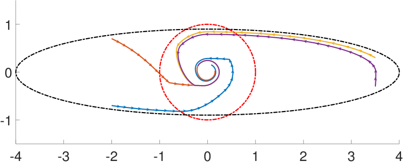
We present three numerical examples to demonstrate the efficacy of the proposed methods. In the first scenario, we consider the example of reaching a set in a prescribed time , and stay there for all future times, while also remaining in a at all times. Mathematically, the closed-loop trajectories are required to satisfy , with . The system dynamics are considered as
where the state-vector is and the control input is . Note that the open-loop trajectories for these dynamics diverge to infinity, i.e., the origin is unstable for the open-loop system. We choose and and sec. Figure 2 shows the closed-loop trajectories for four different initial conditions. The trajectories reach the set in prescribed time and stay there at all the future times, while remaining in the set at all times.
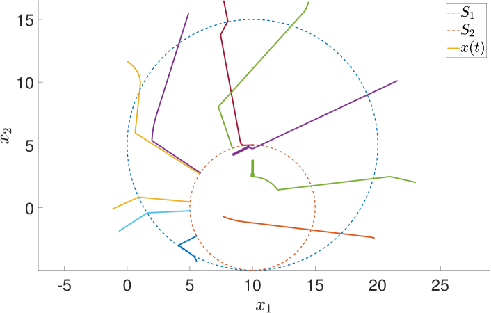
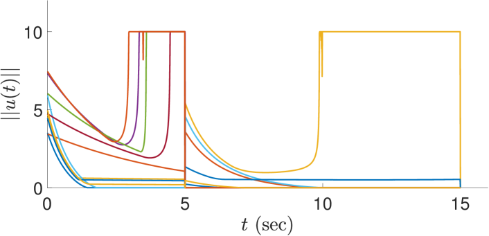
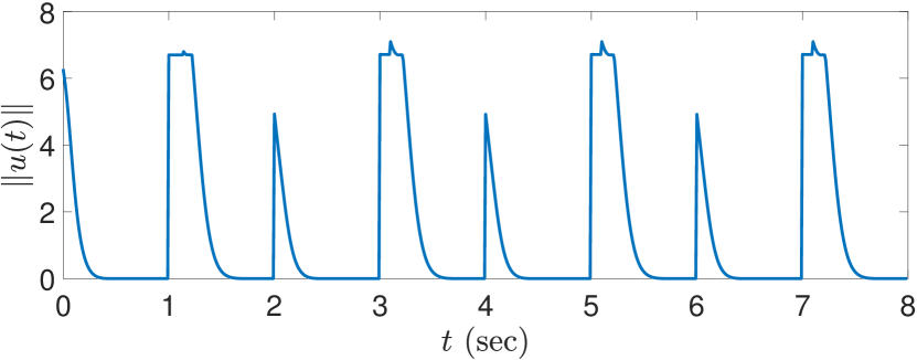
In second scenario, we take Example 2 from [18] and use our proposed method to satisfy the STL specifications , where and , with and . The robot dynamics are modeled as where . We use as the control input constraints. In order to translate the input constraint in the form of (16e), we define and , so that . Figure 3 shows the closed-loop trajectories for various initial conditions outside the set . It can be seen that the trajectories reach the set and stay in at all future times, and then reach set . Figure 4 shows the norm of the control input with time. As can be seen from the figure, the control input jumps at sec, when the system trajectories reach the set .
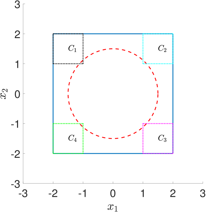
In the third scenario, we present a method of constructing sets for applications such as robot motion planning, where the conditions of Theorem 4 are not met. The closed-loop trajectories, starting from , are required to satisfy the following spatio-temporal specifications, which is explained in details below (see Figure 5):
-
•
for all , i.e., the closed-loop trajectories should stay inside the solid-blue square and outside the red-dotted circle at all times;
-
•
Before a given , ;
-
•
Before a given , ;
-
•
Before a given , ;
-
•
Before a given , .
This problem is an extended version of the case study considered in [24]. Note that the sets are not overlapping with each other, and the corresponding functions are not continuously differentiable. Now, in order to be able to use QP-based formulation (16), we need to find the sets such that .
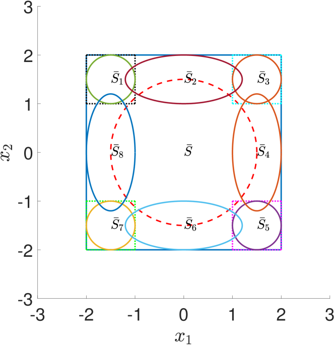
The set and sets are defined as follows (see Figure 6):
-
•
;
-
•
;
-
•
;
-
•
;
-
•
;
-
•
;
-
•
;
-
•
;
where and . The problem can be re-formulated to design a control input such that for ,
-
•
For a given , ;
-
•
For a given , ;
-
•
For a given , ;
-
•
For a given , ;
-
•
For a given , ;
-
•
For a given , ;
-
•
For a given , ;
-
•
For a given , ,
which can be written as an STL formula as in (V).
| (18) |
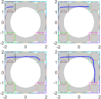
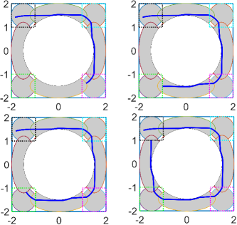
We can now use the formulation (16) to compute the control input. We use as the input constraints and use the same approach as in scenario 2, to translate these constraints in the form of (16e). The time constraints are chosen as for and for . We choose , so that and . Figures 8-8 illustrate the closed-loop position trajectories of the robot for one initial condition; it is evident that the robot position always remains in the safe set , while visiting the sets and sequentially.Figure 9 illustrates the control input trajectories and verifies that the control input constraint is satisfied at all times.
VI Direction for future work
Note that Theorem 2, Corollary 1 and Theorem 4 are restrictive because of the following two reasons. First, it is needed that the functions and are CLF/CBF for the system (4), otherwise the respective inequalities used in the aforementioned results do not hold. Second, these results also need that the functions and are continuously differentiable. Although, this is a very common assumption in the literature (see [8, 11] and other similar work), this limits the choice of sets and that can be considered in the setup of Theorem 2 or Theorem 4. One approach is to use non-smooth analysis (e.g., [25]) to formulate the constraints of (16), so that the sets characterized by non-differentiable can also be incorporated. Another plausible approach is to look for the CLF and the control input simultaneously. We propose sufficient conditions to characterize the CLF and the control input for Problem 1.
Proposition 1.
If there exist continuously differentiable function and constants , and satisfying such that the following holds for
| (19a) | ||||
| (19b) | ||||
where , then the closed-loop trajectories of (4) reach the set within prescribed time for all initial conditions.
Proof.
We illustrate, via a simple example, how Proposition 1 can be used for the case when is non-smooth. Consider the case when the set in Problem 1 is defined as , i.e., using the 1-norm of , so that is a square. Using the fact that , as , one can choose , for large positive integer and look for , along with , and so that conditions of Proposition 1 hold. A similar set of sufficient conditions can be derived for Theorem 4, which would allow a larger class of problems to be solved. It is part of our future investigations to study methods to solve for and , simultaneously, in an efficient way. In future, we would also like to study properties of the system dynamics and the functions , so that the resulting closed-loop trajectories are smooth.
VII Conclusions
In this paper, we considered the problem of trajectory planning under spatio-temporal, and control input constraints. We defined a new class of CLF, called PT CLF, to guarantee that the closed loop trajectories reach a given set within the prescribed time. We formulated a QP to find a control input that guarantees prescribed time convergence. Then, we considered a general problem of control synthesis under multiple spatiotemporal objectives. We first presented sufficient conditions for the existence of a control input in terms of PT CLF and CBF. Then, we presented a QP based formulation to efficiently compute the control input that guarantees safety and prescribed time convergence in the presence of control input constraints.
References
- [1] M. Saska, Z. Kasl, and L. Přeucil, “Motion planning and control of formations of micro aerial vehicles,” IFAC Proceedings Volumes, vol. 47, no. 3, pp. 1228–1233, 2014.
- [2] A. Grancharova, E. I. Grøtli, D.-T. Ho, and T. A. Johansen, “Uavs trajectory planning by distributed mpc under radio communication path loss constraints,” Journal of Intelligent & Robotic Systems, vol. 79, no. 1, pp. 115–134, 2015.
- [3] M. Svenstrup, T. Bak, and H. J. Andersen, “Trajectory planning for robots in dynamic human environments,” in 2010 IEEE/RSJ International Conference on Intelligent Robots and Systems. IEEE, 2010, pp. 4293–4298.
- [4] L. Palmieri, S. Koenig, and K. O. Arras, “Rrt-based nonholonomic motion planning using any-angle path biasing,” in 2016 IEEE International Conference on Robotics and Automation (ICRA). IEEE, 2016, pp. 2775–2781.
- [5] O. Salzman and D. Halperin, “Asymptotically near-optimal rrt for fast, high-quality motion planning,” IEEE Transactions on Robotics, vol. 32, no. 3, pp. 473–483, 2016.
- [6] B. Kovács, G. Szayer, F. Tajti, M. Burdelis, and P. Korondi, “A novel potential field method for path planning of mobile robots by adapting animal motion attributes,” Robotics and Autonomous Systems, vol. 82, pp. 24–34, 2016.
- [7] D. Han and D. Panagou, “Robust multi-task formation control via parametric lyapunov-like barrier functions,” IEEE Transactions on Automatic Control, 2019.
- [8] A. Li, L. Wang, P. Pierpaoli, and M. Egerstedt, “Formally correct composition of coordinated behaviors using control barrier certificates,” in 2018 IEEE/RSJ International Conference on Intelligent Robots and Systems. IEEE, 2018, pp. 3723–3729.
- [9] M. Srinivasan, S. Coogan, and M. Egerstedt, “Control of multi-agent systems with finite time control barrier certificates and temporal logic,” in 2018 IEEE Conference on Decision and Control. IEEE, 2018, pp. 1991–1996.
- [10] A. D. Ames, K. Galloway, and J. W. Grizzle, “Control lyapunov functions and hybrid zero dynamics,” in 2012 IEEE 51st IEEE Conference on Decision and Control. IEEE, 2012, pp. 6837–6842.
- [11] A. D. Ames, X. Xu, J. W. Grizzle, and P. Tabuada, “Control barrier function based quadratic programs for safety critical systems,” IEEE Transactions on Automatic Control, vol. 62, no. 8, pp. 3861–3876, 2017.
- [12] X. Xu, P. Tabuada, J. W. Grizzle, and A. D. Ames, “Robustness of control barrier functions for safety critical control,” IFAC-PapersOnLine, vol. 48, no. 27, pp. 54–61, 2015.
- [13] A. J. Barry, A. Majumdar, and R. Tedrake, “Safety verification of reactive controllers for uav flight in cluttered environments using barrier certificates,” in International Conference on Robotics and Automation. IEEE, 2012, pp. 484–490.
- [14] A. D. Ames, J. W. Grizzle, and P. Tabuada, “Control barrier function based quadratic programs with application to adaptive cruise control,” in 53rd Annual Conference on Decision and Control. IEEE, 2014, pp. 6271–6278.
- [15] M. Z. Romdlony and B. Jayawardhana, “Stabilization with guaranteed safety using control lyapunov–barrier function,” Automatica, vol. 66, pp. 39–47, 2016.
- [16] K. P. Tee, S. S. Ge, and E. H. Tay, “Barrier lyapunov functions for the control of output-constrained nonlinear systems,” Automatica, vol. 45, no. 4, pp. 918–927, 2009.
- [17] M. Rauscher, M. Kimmel, and S. Hirche, “Constrained robot control using control barrier functions,” in 2016 IEEE/RSJ International Conference on Intelligent Robots and Systems (IROS). IEEE, 2016, pp. 279–285.
- [18] L. Lindemann and D. V. Dimarogonas, “Control barrier functions for signal temporal logic tasks,” IEEE control systems letters, vol. 3, no. 1, pp. 96–101, 2019.
- [19] S. P. Bhat and D. S. Bernstein, “Finite-time stability of continuous autonomous systems,” SICON, vol. 38, no. 3, pp. 751–766, 2000.
- [20] A. Polyakov, “Nonlinear feedback design for fixed-time stabilization of linear control systems,” IEEE Transactions on Automatic Control, vol. 57, no. 8, p. 2106, 2012.
- [21] J. C. Holloway and M. Krstic, “Prescribed-time observers for linear systems in observer canonical form,” IEEE Transactions on Automatic Control, 2019.
- [22] Y. Li and R. G. Sanfelice, “Finite time stability of sets for hybrid dynamical systems,” Automatica, vol. 100, pp. 200–211, 2019.
- [23] A. D. Ames, K. Galloway, K. Sreenath, and J. W. Grizzle, “Rapidly exponentially stabilizing control lyapunov functions and hybrid zero dynamics,” IEEE Transactions on Automatic Control, vol. 59, no. 4, pp. 876–891, 2014.
- [24] L. Lindemann and D. V. Dimarogonas, “Robust motion planning employing signal temporal logic,” in 2017 American Control Conference. IEEE, 2017, pp. 2950–2955.
- [25] E. Sontag and H. J. Sussmann, “Nonsmooth control-lyapunov functions,” in Proceedings of 1995 34th IEEE Conference on Decision and Control, vol. 3. IEEE, 1995, pp. 2799–2805.