Thermodynamic Properties of Graphene in Magnetic Field
and Rashba Coupling

Rachid Houça^a,b, Ahmed Jellal^b

^aEquipe de Physique Théorique et Hautes Energies, Faculté des Sciences, Université Ibn Zohr,

PO Box 8106, Agadir, Maroc

^bLaboratory of Theoretical Physics, Faculty of Sciences, Chouaïb Doukkali University,

PO Box 20, 24000 El Jadida, Morocco

We study the thermodynamic properties of massless Dirac fermions in graphene subjected to a uniform magnetic field $B$ together with Rashba coupling parameter $\lambda_{R}$. The thermodynamic functions such as the Helmholtz free energy, total energy, entropy and heat capacity are obtained in the high temperature regime using an approach based on the zeta function. These functions will be numerically examined by considering two cases related to $\lambda_{R}$ smaller or greater than $B$. In particular, we show that the Dulong-Petit law is verified for both cases.

PACS numbers: 65.80.Ck

Keywords: Graphene, Rashba coupling, zeta function, partition function, thermodynamic functions.

1 Introduction

Graphene is a two-dimensional system formed by a plane of carbon atoms arranged in a honeycomb structure [1, 2]. Since it isolation in 2004, the rise of this material is growing because its electronic and mechanical properties are interesting. In particular, graphene is the material having the greatest electrical mobility at ambient temperature [3, 4]. It is also very flexible, extremely strong and is an excellent thermal conductor. These properties give graphene incredible potential for many applications in the fields of electronics, composite materials, energy storage. The transition from laboratory to industry is primarily based on the possibility of producing graphene on a large scale and at a reasonable cost.

Nowadays, graphene-based systems have no particular utility in magnetic information storage applications or in spintronics [5, 6], mainly because of the absence of magnetic moments in carbon and the negligible interaction between the spin of electrons with the movement of electronic charges (spin-orbit coupling) [7]. This situation changes radically when graphene is interfaced with other materials by creating a heterostructure, that will offer the possibility of manipulating the spin of the electron for graphene via the spin-orbit coupling which can be controlled by the application of an electric field in the transverse direction of gas [8, 9]. This property has generated considerable research activity due to possible applications in the emerging field of spintronics. An interesting direction of research is to combine the spin-orbit coupling of Rashba with the thermodynamic properties of graphene [10, 11]. On the theoretical level, it is necessary to better understand the combined effects of an intense electric field of spin-orbit coupling, confinement and disorder potentials [12, 13, 14], which have a direct bearing on the charge transport and spin properties of the electron that reflect on thermodynamic quantities.

Thermodynamic properties of graphene based on the statistical physics formalism was the subject of different investigations. Indeed, the thermodynamic properties of graphene nanoribbons under zero and finite magnetic fields have been investigated [15]. The electronic states in the tight-binding approximation were used to calculate the thermal and magnetic properties. In the case of a finite magnetic field, the Harper equation was solved for the electronic state for various wavevectors. The magnetic field and temperature dependence of the magnetic susceptibility over a wide field and temperature range were presented. Thermodynamic properties of a weakly modulated graphene monolayer in a magnetic field was analyzed in [16] and found that the modulation-induced effects on the thermodynamic properties are enhanced and less damped with temperature in graphene compared with conventional 2DEG systems.

We study the thermodynamic properties of Dirac fermions in graphene subjected to an uniform magnetic field with the Rashba coupling parameter. After getting the solutions of the energy spectrum, we use the zeta function to explicitly determine the partition function that will be used to calculate the Helmholtz free energy, total energy, entropy and specific heat. These will be numerically analyzed by considering two cases of $\lambda_{R}$ smaller/greater than $B$ under suitable conditions of the physical parameters. We show that the so-called Dulong-Petit law can be recovered as a limiting case from our results.

The manuscript is organized as follows. In section $2$, we formulate our problem by introducing the bosonic operators and choosing a convenient gauge to diagonalize the corresponding Hamiltonian. The partition function of the system will be determined via an approach based on zeta function and the thermodynamic functions that describe the thermal physics of monolayer graphene with Rashba coupling will be calculated in section $3$. Section 4 will be devoted to the numerical results and discussions as well as comparison with literature. We conclude our results in the final section.

2 Theoretical model

To study the thermodynamic proprieties of graphene subjected to an uniform magnetic field with Rashba coupling, we consider the tight-binding model together with Rashba term. This is governed by the Hamiltonian

$$H=H_{0}+H_{R}$$ (1)

where the first term is given by [17]

$$H_{0}=-t\sum_{\langle i,j\rangle,\alpha}a_{i,\alpha}^{\dagger}a_{j,\alpha}$$ (2)

$a_{i,\alpha}^{\dagger}$ and $a_{j,\alpha}$ are the creation and annihilation operators of fermions placed on the site $i$, $\alpha$ labels the spin and $t\simeq 2,8eV$ is the intralayer hopping parameter between nearest-neighbor sites. The Rashba Hamiltonian for nearest-neighbor hopping reads as [18]

$$H_{R}=it_{R}\sum_{\langle i,j\rangle}a_{i}^{\dagger}\vec{z}\left(\vec{s}\times\vec{d}_{i,j}\right)a_{j}$$ (3)

where $\vec{d}_{i,j}$ is the lattice vector pointing from site $j$ to site $i$, $\vec{s}$ is a vector whose elements are the Pauli matrices in the spin space, the spin-orbit coupling $t_{R}$ is determined by the strength of the electric field, $a_{i}^{\dagger}=\left(a_{i,\uparrow}^{\dagger},a_{i,\downarrow}^{\dagger}\right)$ are vectors in the spin space [19]. Expanding the Hamiltonian (1) in the vicinity of the valleys $\vec{K}_{\pm}=(\pm\frac{4\pi}{3}\sqrt{3},0)$, gives the low-energy Hamiltonian in the sublattice $(A,B)$ and spin $(\uparrow,\downarrow)$ spaces

$$H=v_{F}\left(\eta\sigma_{x}\pi_{x}+\sigma_{y}\pi_{y}\right)+\lambda_{R}\left(\eta\sigma_{x}s_{y}-\sigma_{y}s_{x}s\right)$$ (4)

where the conjugate momentum $\pi_{x}$ and $\pi_{y}$ can be written in symmetric gauge $\vec{A}=\frac{B}{2}(-y,x)$ as

$$\pi_{x}=p_{x}-\frac{eB}{2}y,\qquad\pi_{y}=p_{y}+\frac{eB}{2}x.$$ (5)

the Fermi velocity $v_{F}=\frac{3at}{2\hbar}$ with $a=1.142nm$, $\eta=\pm 1$ labels the valley degrees of freedom, $\sigma=\left(\sigma_{x},\sigma_{y}\right)$ are the Pauli matrices of pseudospin operator on $A(B)$ lattice cites. Note that the present system also presents the intrinsic spin orbit coupling (SOC), but its value is very weak $\sim 12\mu eV$ [19] compared to the Rashba coupling parameter $\lambda_{R}=\frac{\hbar veE}{4mc^{2}}$ [20], which depends on the external electric field perpendicular to the graphene plane is very strong compared to intrinsic SOC.

The Hamiltonian (4) around a single Dirac point $(\eta=+1)$ on the double-spinor basis $|\Psi\rangle=(|r_{A},n,\uparrow\rangle,|r_{B},n-1,\downarrow\rangle,|r_{B},n,\uparrow\rangle,|r_{A},n-1,\downarrow\rangle)^{t}$ is given by

$$H=\left(\begin{array}[]{cccc}0&0&v\left(\pi_{x}-i\pi_{y}\right)&0\\ 0&0&0&v\left(\pi_{x}+i\pi_{y}\right)\\ v\left(\pi_{x}+i\pi_{y}\right)&0&0&-2i\lambda_{R}\\ 0&v\left(\pi_{x}-i\pi_{y}\right)&2i\lambda_{R}&0\\ \end{array}\right).$$ (6)

To diagonalize the Hamiltonian (6), it is convenient to introduce the usual bosonic operators in terms of the conjugate momentum

$$a=\frac{\ell_{B}}{\sqrt{2}\hbar}\left(\pi_{x}-i\pi_{y}\right),\qquad a^{\dagger}=\frac{\ell_{B}}{\sqrt{2}\hbar}\left(\pi_{x}+i\pi_{y}\right)$$ (7)

which verify the commutation relation $[a,a^{\dagger}]=\mathbb{I}$, $\ell_{B}=\sqrt{\frac{\hbar}{eB}}$ is the magnetic length. Mapping (6) in terms of $a$ and $a^{\dagger}$ to end up with

$$H=\left(\begin{matrix}0&0&\frac{\sqrt{2}\hbar v}{\ell_{B}}a&0\\ 0&0&0&\frac{\sqrt{2}\hbar v}{\ell_{B}}a^{\dagger}\\ \frac{\sqrt{2}\hbar v}{\ell_{B}}a^{\dagger}&0&0&-2i\lambda_{R}\\ 0&\frac{\sqrt{2}\hbar v}{\ell_{B}}a&2i\lambda_{R}&0\\ \end{matrix}\right).$$ (8)

To obtain the solution of the energy spectrum we act the Hamiltonian on the state $|\Psi\rangle$ leading to the eigenvalue equation

$$\left(\begin{matrix}-E&0&\frac{\sqrt{2}\hbar v}{\ell_{B}}a&0\\ 0&-E&0&\frac{\sqrt{2}\hbar v}{\ell_{B}}a^{\dagger}\\ \frac{\sqrt{2}\hbar v}{\ell_{B}}a^{\dagger}&0&-E&-2i\lambda_{R}\\ 0&\frac{\sqrt{2}\hbar v}{\ell_{B}}a&2i\lambda_{R}&-E\\ \end{matrix}\right)\left(\begin{matrix}|r_{A},n,\uparrow\rangle\\ |r_{B},n-1,\downarrow\rangle\\ |r_{B},n,\uparrow\rangle\\ |r_{A},n-1,\downarrow\rangle\\ \end{matrix}\right)=\left(\begin{matrix}0\\ 0\\ 0\\ 0\\ \end{matrix}\right)$$ (9)

giving rise to the following set

$$-E|r_{A},n,\uparrow\rangle+\frac{\sqrt{2}\hbar v}{\ell_{B}}a|r_{B},n,\uparrow\rangle=0$$ (10)

$$-E|r_{B},n-1,\downarrow\rangle+\frac{\sqrt{2}\hbar v}{\ell_{B}}a^{\dagger}|r_{A},n-1,\downarrow\rangle=0$$ (11)

$$\frac{\sqrt{2}\hbar v}{\ell_{B}}a^{\dagger}|r_{A},n,\uparrow\rangle-E|r_{B},n,\uparrow\rangle-2i\lambda_{R}|r_{A},n-1,\downarrow\rangle=0$$ (12)

$$\frac{\sqrt{2}\hbar v}{\ell_{B}}a|r_{B},n-1,\downarrow\rangle+2i\lambda_{R}|r_{B},n,\uparrow\rangle)-E|r_{A},n-1,\downarrow\rangle=0.$$ (13)

These can be solved to obtain a second order equation for the eigenvalues

$$E^{2}\pm 2\lambda_{R}E-\left(\hbar\omega_{D}\right)^{2}n=0,\qquad n=0,1,2\cdots$$ (14)

where $\omega_{D}=v_{F}\sqrt{\frac{2eB}{\hbar}}$ is the Dirac constant. A straightforward calculation leads to the following solutions

$$E_{1,n}^{\pm}=-\lambda_{R}\pm\sqrt{\lambda_{R}^{2}+\left(\hbar\omega_{D}\right)^{2}n}$$ (16)

$$E_{2,n}^{\pm}=\lambda_{R}\pm\sqrt{\lambda_{R}^{2}+\left(\hbar\omega_{D}\right)^{2}n}$$

These are four band solutions and are strongly dependent on the Rashba coupling parameter $\lambda_{R}$, which reduces to two bands once $\lambda_{R}$ is switched off. As it will be shown, this parameter will play a crucial role in the forthcoming study. Next we will see how the above results can be employed to explicitly determine in the first stage the partition function and in the second one derive the related thermodynamic functions.

3 Thermodynamic functions

We will study the thermodynamic properties of the monolayer graphene with Rashba coupling in contact with a thermal reservoir at finite temperature. For simplicity, we assume that only fermions with positive energy $(E>0)$ are regarded to constitute the thermodynamic ensemble [21]. We start by evaluating the corresponding partition function

$$\mathbb{Z}={\rm Tr}e^{-\beta H}=\sum_{n=0}^{+\infty}\left(e^{-\beta E_{1,n}^{+}}+e^{-\beta E_{2,n}^{+}}\right)$$ (17)

where $\beta=\frac{1}{k_{B}T}$, $k_{B}$ is the Boltzmann constant and $T$ is the equilibrium temperature. Using (16-17) and after some algebra, we show that $\mathbb{Z}$ takes the form

$$\mathbb{Z}=2\cosh(\beta\lambda_{R})\sum_{n=0}^{+\infty}e^{-\beta\sqrt{\left(\hbar\omega_{D}\right)^{2}n+\lambda_{R}^{2}}}.$$ (18)

To go further, let us make the following changes

$$r=\left(\frac{\hbar\omega_{D}}{\lambda_{R}}\right)^{2},\qquad\gamma=\sqrt{r}=\frac{\hbar\omega_{D}}{\lambda_{R}},\qquad\kappa=\frac{1}{r},\qquad\tau=\frac{k_{B}T}{\lambda_{R}}$$ (19)

which can be used to write $\mathbb{Z}$ as

$$\mathbb{Z}=2\cosh(\beta\lambda_{R})\sum_{n=0}^{+\infty}e^{-\frac{\gamma}{\tau}\sqrt{n+\kappa}}.$$ (20)

Now considering the integral formula [22]

$$e^{-x}=\frac{1}{2\pi i}\int_{C}x^{-s}\Gamma(s)ds$$ (21)

to convert the sum in (20) as

$$\sum_{n=0}^{+\infty}e^{-\frac{\gamma}{\tau}\sqrt{n+\kappa}}=\frac{1}{2\pi i}\int_{C}\left(\frac{\gamma}{\tau}\right)^{-s}\sum_{n}(n+\kappa)^{-\frac{s}{2}}\Gamma(s)=\frac{1}{2\pi i}\int_{C}\left(\frac{\gamma}{\tau}\right)^{-s}\sum_{n}\xi_{H}\left(\frac{s}{2},\kappa\right)\Gamma(s)$$ (22)

with two zeta functions of Euler $\Gamma$ and Hurwitz $\xi_{H}$. The function $\xi_{H}$ is defined for complex arguments $s$ (with $\Re(s)>1$) and $\kappa$ (with $\Re(\kappa)>0$), it is absolutely convergent for given values of $s$ and $\kappa$, which can be extended to a meromorphic function defined for all $s\neq 1$. To calculate the sum (22) we apply the residue theorem for the poles $s=0$ and $s=2$ to get

$$\sum_{n=0}^{+\infty}e^{-\frac{\gamma}{\tau}\sqrt{n+\kappa}}=\left(\frac{\tau}{\gamma}\right)^{2}+\xi_{H}\left(0,\kappa\right)$$ (23)

where $\xi_{H}\left(0,\kappa\right)=\frac{1}{2}-\kappa$. Combining all to end up with the partition function

$$\mathbb{Z}=2\left(\frac{(k_{B}T)^{2}-\lambda_{R}^{2}}{(\hbar\omega_{D})^{2}}+\frac{1}{2}\right)\cosh\beta\lambda_{R}.$$ (24)

By virtue of the stability of the graphene at high temperature [23] we will study its thermodynamic properties to make a comparison with other studies. Indeed, in the limit $k_{B}T\gg\lambda_{R}$, the total partition function $\mathbb{Z}_{N}$ for $N$ fermions can be approximated by

$$\mathbb{Z}_{N}\simeq\left(\left(2\left(\frac{1}{\beta\hbar\omega_{D}}\right)^{2}+1\right)\cosh\beta\lambda_{R}\right)^{N}.$$ (25)

We point out that several studies have been developed on graphene using formalism based on zeta function. Among them, we cite work reported by Beneventano et al. [24] in studying the quantum Hall effect, Berry’s phases and minimal conductivity of graphene. Also Falomir et al. [25] evaluated the Hall conductivity of the model from the partition function employing the zeta function approach to the associated functional determinant.

Since we have derived the partition function of our system, we can now determine all related thermodynamic functions. Indeed, after some algebras we obtain the Helmholtz free energy $F$, total energy $U$, entropy $S$ and specific heat $C$

$$\frac{F}{N}=-\frac{1}{\beta}\ln\mathbb{Z}=-\frac{1}{\beta}\ln\left(\frac{2}{\beta^{2}\hbar^{2}\omega_{D}^{2}}+1\right)-\frac{1}{\beta}\ln\left(\cosh(\beta\lambda_{R})\right)$$ (26)

$$\frac{U}{N}=-\frac{\partial}{\partial\beta}\ln\mathbb{Z}=\frac{4-\beta\lambda_{R}\left(\beta^{2}\hbar\omega_{D}^{2}+2\right)\tanh(\beta\lambda_{R})}{\beta\left(\beta^{2}\hbar^{2}\omega_{D}^{2}+2\right)}$$ (29)

$$\frac{S}{Nk_{B}}=\beta^{2}\frac{\partial F}{\partial\beta}=-\beta\lambda_{R}\left(\tanh(\beta\lambda_{R})\right)+\ln\left(\frac{2}{\beta^{2}\hbar^{2}\omega_{D}^{2}}+1\right)\cosh(\beta\lambda_{R})+\frac{4}{\beta^{2}\hbar^{2}\omega_{D}^{2}+2}$$

$$\frac{C}{Nk_{B}}=-\beta^{2}\frac{\partial U}{\partial\beta}=\frac{\beta^{2}\lambda_{R}^{2}\left(\beta^{2}\hbar^{2}\omega_{D}^{2}+2\right)^{2}\text{sech}^{2}(\beta\lambda_{R})+12\beta^{2}\hbar^{2}\omega_{D}^{2}+8}{\left(\beta^{2}\hbar^{2}\omega_{D}^{2}+2\right)^{2}}.$$

Next, we will numerically analyse the above thermodynamic functions to underline the behavior of our system. This will be done by giving some plots under suitable conditions and making different discussions.

4 Numerical results and discussions

We recall our theory includes two interesting quantities, which are the Rashba coupling parameter $\lambda_{R}$ and the external magnetic field $B$. To carry out our numerical study, we consider the case when the ratio $\frac{\lambda_{R}}{\hbar\omega_{D}}$ is smaller or greater than one. Indeed, For a smaller ratio than one, the thermodynamic functions versus the temperature $k_{B}T$ for the fixed values $\hbar\omega_{D}=10\lambda_{R},20\lambda_{R},30\lambda_{R},40\lambda_{R}$. It is clearly seen that in Figure 1(a) the Helmontz function $\frac{F}{N}$ has a little increase when $k_{B}T$ starts to increase, but it decreases rapidly for high values of $k_{B}T$. For the four fixed values $\frac{F}{N}$ is showing the same behavior except that the velocity of decrease changes, which means that we can increase/decrease $\frac{F}{N}$ by tuning on $\lambda_{R}$. In Figure 1(b) for the interval $0<k_{B}T<5$ we observe that the behavior of the total energy $\frac{U}{N}$ is independent on different values of $\lambda_{R}$ while in the interval $5<k_{B}T<40$ it starts increasing with a nearly linear behavior. The entropy $\frac{S}{N}$ is slowly increasing for large $k_{B}T$ and decreases for strong values of $\lambda_{R}$ as shown in Figure 1(c). In Figure 1(d) the heat capacity $\frac{C}{Nk_{B}}$ is showing that there is a peak appearing with small values of $\lambda_{R}$ and it tends to an asymptotic behavior fixed in the value $2$ when $k_{B}T$ increases.

In Figure 2 we investigate the second case by shooing the values of the Rashba coupling parameters $\lambda_{R}=10\hbar\omega_{D}$, $20\hbar\omega_{D}$, $30\hbar\omega_{D},40\hbar\omega_{D}$. From Figure 2(a) We observe that the Helmontz function $\frac{F}{N}$ decreases when $k_{B}T>2$ and changes as long as $\lambda_{R}$ increases. The total energy $\frac{U}{N}$ increases with almost a linear behavior when $0<k_{B}T<20$ but faraway we observe that it shows the same behavior for any value of $\lambda_{R}$ as depicted in Figure 2(b). In Figure 2(c), the entropy $\frac{S}{N}$ is independent on the parameter $\lambda_{R}$ in the interval $0<k_{B}T<5$, but when $k_{B}T>5$, $\frac{S}{N}$ shows a small variation in terms of $\lambda_{R}$. The heat capacity $\frac{C}{Nk_{B}}$ does not change with respect to the first case, which has constantly asymptotic behavior in the value $2$ for the high temperature regime as shown in Figure 2(d).

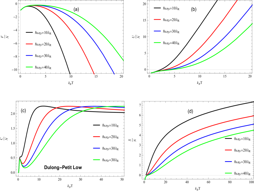
Figure 1: (Color online) Thermodynamic functions of Dirac fermions in graphene with Rashba coupling $\lambda_{R}$ and magnetic field $B$ versus the temperature $k_{B}T$ for the values $\hbar\omega_{D}=10\lambda_{R},20\lambda_{R},30\lambda_{R},40\lambda_{R}$. (a): The Helmholtz free energy, (b): the mean energy, (c): the entropy, (d): the heat capacity.

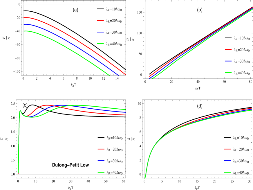
Figure 2: (Color online) Thermodynamic functions of Dirac fermions in graphene with Rashba coupling $\lambda_{R}$ and magnetic field $B$ versus the temperature $k_{B}T$ for the values $\lambda_{R}=10\hbar\omega_{D},20\hbar\omega_{D},30\hbar\omega_{D},40\hbar\omega_{D}$. (a): The Helmholtz free energy, (b): the mean energy, (c): the entropy, (d): the heat capacity.

By examining the thermodynamic properties for monolayer graphene with Rashba coupling, we observe that the average energy for our system presents a critical point for low temperature, that is, near $T=0K$. However, the temperature of the system increases, the amount of free energy available to perform the ensemble work decreases rapidly. In contrast, we notice that when this ensemble tends to the thermal equilibrium in the reservoir, the internal energy of the system increases continuously. The thermal variation of the system tends to increase until reaching the thermal equilibrium, where it becomes constant. Moreover, based on the solid state physics, we notice that the well-known Dulong-Petit law is satisfied for our system, which is characterized by $\frac{C}{N}=2k_{B}$ [21] as seen in both Figures 1(c) and 2(c).

5 Conclusion

We have studied the thermodynamic properties of a massless Dirac fermions in graphene subjected to an uniform magnetic field with Rashba interaction. The annihilation and creation operators were introduced to obtain the solutions of the energy spectrum. These are used together with a method based on the zeta function to explicitly determine the partition function. Therefore the thermodynamic functions such as the Helmholtz free energy, total energy, entropy and heat capacity were obtained in terms of the Rashba coupling parameter.

Subsequently, two cases have been studied related to Rashba coupling parameter $\lambda_{R}$ and magnetic filed $B$ in the high temperature regime. Indeed, we have analyzed numerically the case when $\lambda_{R}$ is smaller than $B$, which allowed us to recover a result already obtained in [21] for graphene system. We have also considered the case when $\lambda_{R}$ is greater than $B$ where it was shown that the Dulong– Petit law is always verified by our system.

References

- [1] K. S. Novoselov, A. K. Geim, S. V. Morozov, D. Jiang, Y. Zhang, S. V. Dubonos, I. V. Grigorieva, and A. A. Firsov, Science. 306, 666 (2004).
- [2] C. Berger, Z. Song, T. Li, X. Li, A. Y. Ogbazghi, R. Feng, Z. Dai, A. N. Marchenkov, E. H. Conrad, P. N. First, and W. A. de Heer, J. Phys. Chem. B 108, 19912 (2004).
- [3] K. I. Bolotin, K. J. Sikes, Z. Jiang, M. Klima, G. Fudenberg, J. Hone, P. Kim, and H. L. Stormer, Solid State Commun. 146, 351 (2008).
- [4] J. H. Chen, C, Jang, S. Xiao, M. Ishigami, and M. S. Fuhrer, Nat. Nanotechnol. 3, 206 (2008).
- [5] H. Dery, P. Dalal, L. Cywinski, and L. J. Sham, Nature 447, 573 (2007).
- [6] S. Datta and B. Das, Appl. Phys. Lett. 56, 665 (1990).
- [7] D. Huertas-Hernando, F. Guinea, and A. Brataas, Phys. Rev. Lett. 103, 146801 (2009).
- [8] E. I. Rashba, Sov. Phys. Solid State 2, 1109 (1960).
- [9] Y. A. Bychkov and E. I. Rashba, J. Phys. C 17, 6039 (1984).
- [10] A. A. Balandin, Nature Mater. 10, 569 (2011).
- [11] A. I. Rusanov, Surface Science Reports 69, 296 (2014).
- [12] J. Nitta, T. Akazaki, H. Takayanagi, and T. Enoki, Phys. Rev. Lett. 78, 1335 (1997).
- [13] J. P. Heida, B. J. van Wees, J. J. Kuipers, T. M. Klapwijk, and G. Borghs, Phys. Rev. B 57, 11911 (1998).
- [14] S. J. Papadakis, E. P. DePoortere, H. C. Manoharan, M. Shayegan, and R. Winkler, Science 283, 2056 (1999).
- [15] A. R. Wright, Junfeng Liu, Zhongshui Ma, Z. Zeng, W. Xu, and C. Zhang, Microelectronics Journal 40, 716 (2009).
- [16] R. Nasir, M. A. Khan, M. Tahir, and K. Sabeeh, J. Phys.: Condens. Matter 22 (2010) 025503.
- [17] A. H. Castro Neto, F. Guinea, N. M. R. Peres, K. S. Novoselov, and A. K. Geim, Rev. Mod. Phys. 81, 109 (2009).
- [18] Z. Qiao, H. Jiang, X. Li, Y. Yao, and Q. Niu, Phys. Rev. B 85, 115439 (2012).
- [19] S. Konschuh, M. Gmitra, and J. Fabian, Phys. Rev. B 82, 245412 (2010).
- [20] C. L. Kane and E. J. Mele, Phys. Rev. Lett. 95, 226801 (2005).
- [21] V. Santos, R. V. Maluf and C. A. S. Almeida, Ann. Phys. 349, 402 (2014).
- [22] Marina-Aura Dariescu and C. Dariescu, J. Phys: Condens. Matter 19, 256203 (2007); ibid, Chaos Solitons and Fractals 33, 776 (2007).
- [23] Kwanpyo Kim, William Regan, Baisong Geng, Benjamín Alemán, B. M. Kessler, Feng Wang, M. F. Crommie, and A. Zettl Phys. Status Solidi RRL 4, 302 (2010).
- [24] C. G. Beneventano, P. Giacconi, E. M. Santangelo, and R. Soldati, J. Phys. A: Math. Theor. 40, 435 (2007).
- [25] H. Falomir, J. Gamboa, M. Loewe and M. Nieto, J. Phys. A: Math. Theor. 45, 135308 (2012).