Robust Super-resolution GAN, with Manifold-Based and Perception Loss

Abstract

Super-resolution using deep neural networks typically relies on highly curated training sets that are often unavailable in clinical deployment scenarios. Using loss functions that assume Gaussian-distributed residuals makes the learning sensitive to corruptions in clinical training sets. We propose novel loss functions that are robust to corruptions in training sets by modeling heavy-tailed non-Gaussian distributions on the residuals. We propose a loss based on an autoencoder-based manifold-distance between the super-resolved and high-resolution images, to reproduce realistic textural content in super-resolved images. We propose to learn to super-resolve images to match human perceptions of structure, luminance, and contrast. Results on a large clinical dataset shows the advantages of each of our contributions, where our framework improves over the state of the art.

Index Terms—  Super-resolution, robustness, generative adversarial network, manifold-based loss, perceptual loss.

1 Introduction and Related Work

Image super-resolution methods generate high-resolution (HR) images from acquired low resolution (LR) images. In many applications, e.g., microscope slide scanning and digital pathology, acquiring LR images can be much faster than acquiring HR images. LR scanning equipment is also cheaper. So, methods that generate high-quality super-resolved (SR) images from LR images can improve productivity in clinical and scientific applications, with much reduced cost.

Learning based approaches have been effective for super-resolution, e.g., early methods using manifold learning [1] and later methods relying on sparse models [2, 3] and random forests [4]. Recent methods leverage deep neural networks (DNNs), e.g., convolutional networks [5, 6] and Laplacian-pyramid networks [7]. DNNs effectively model the rich textural details in HR images and learn complex mapping functions from LR image patches to the corresponding HR patches. A state-of-the-art DNN in super-resolution relies on a generative adversarial network (GAN), namely SRGAN [8]. GANs improve texture modeling in HR patches, and the associated LR-to-HR mapping functions, by using a discriminator in their architecture. During learning, while the discriminator adapts to separate SR images from HR images, the generator adapts to challenge the discriminator by producing SR images that are progressively closer to the HR images.

DNN-based super-resolution [5, 6, 7, 8] relies on high-quality highly curated training sets that entail significant expert supervision (time, effort, cost). In clinical deployment, training sets is far from perfect because of inherent errors in tissue slicing (e.g., tearing), staining (e.g., varying dye concentration), imaging artifacts (e.g., poor focus and contrast, noise), and human mislabeling of data (e.g., mixing images from one organ or imaging modality into another). Typical DNN training uses mean-squared-error (MSE) loss that can make the training very sensitive to (even a small fraction of) atypical, or largely clinically irrelevant, examples present in the training set. MSE-based losses can force the learning, undesirably, to adapt to atypical examples at the cost of the performance on the clinically relevant ones. Thus, we propose novel quasi-norm based losses that are robust to errors in dataset curation by modeling heavy-tailed non-Gaussian probability density function (PDFs) on the residuals.

In addition to penalizing pixel-wise differences, independently, between SR and HR images, we propose to (i) learn the manifold of HR images using an autoencoder and (ii) penalize the manifold-distance between SR and HR images, to capture dissimilarities in textural content (factoring out noise and some artifacts) indicated by inter-pixel dependencies. SRGAN [8] focuses on natural images and uses a VGG-encoding [9] based loss to learn to generate SR images perceptually similar to HR images. For histopathology images, we show that the VGG encoder captures human perception sub-optimally. We propose a loss based on the structural similarity index (SSIM), at a fixed scale, between SR and HR images, to generate SR images that match human perceptions of structure, luminance, and contrast.

We propose a novel GAN-based learning framework for super-resolution that is robust to errors in training-set curation, using quasi-norm based loss functions. In addition to independent pixel-wise losses, we propose to learn the manifold capturing textural characteristics in HR images, by first (pre-)training an autoencoder and then using a robust penalty on dissimilarities between encodings of the SR and HR images. We propose to train our GAN to increase the SSIM (at a fixed scale) to make our SR images being perceptually identical to the HR images. Results on a large clinical dataset shows the benefits of each proposal, where our framework outperforms the state of the art quantitatively and qualitatively.

2 Methods

We describe our novel framework, namely SRGAN_SQE, through its architecture, loss functions, and learning algorithms. Let the random-vector pair $(X^{\text{LR}},X^{\text{HR}})$ model the pair of a LR image patch $X^{\text{LR}}$ and its corresponding HR image patch $X^{\text{HR}}$. Let $P(X^{\text{LR}},X^{\text{HR}})$ be their joint PDF modeling dependencies between the LR-HR patch pairs. The training set has $N$ observed patch pairs $\{(x^{\text{LR}}_{i},x^{\text{HR}}_{i})\}_{i=1}^{N}$, where each $(x^{\text{LR}}_{i},x^{\text{HR}}_{i})$ is drawn independently from $P(X^{\text{LR}},X^{\text{HR}})$. In this paper, LR patches are sized 64$\times$64 pixels and HR (and SR) patches are sized 256$\times$256 pixels.

2.1 Our SRGAN_SQE Architecture

Our SRGAN_SQE (Figure 1(a)) comprises: (i) a generator $\mathcal{G}(\cdot;\theta_{G})$ (Figure 1(b)), (ii) an encoder $\mathcal{E}(\cdot;\theta_{E})$ (Figure 1(c)), and (iii) a discriminator $\mathcal{D}(\cdot;\theta_{D})$ (Figure 1(d)), where $\theta_{G}$, $\theta_{E}$, and $\theta_{D}$ denote the associated trainable parameters.

Generator. Our generator learns a transformation function $\mathcal{G}(\cdot;\theta_{G})$ on LR patches $X^{\text{LR}}$ to transform: (i) the PDF $P(X^{\text{LR}})$ into $P(X^{\text{HR}})$ and (ii) the patch $X^{\text{LR}}$ to the corresponding $X^{\text{HR}}$. The associated loss function penalize the dissimilarity between the SR patch $\mathcal{G}(X^{\text{LR}};\theta_{G})$ and the corresponding HR patch $X^{\text{HR}}$; detailed in Section 2.2. The generator (Figure 1(b)) uses convolutional (conv) layers [10] with relu activation, residual (res) blocks [8], batch-normalization (bn) layers [11], and up-sampling layers (up-spl).

Encoder. To penalize the dissimilarity between the SR patch $\mathcal{G}(X^{\text{LR}};\theta_{G})$ and the corresponding HR patch $X^{\text{HR}}$, we propose a novel architecture to measure and penalize a robust manifold-based distance between the SR and HR patches; detailed in Section 2.2. We learn the manifold, specific to a class of images, in a pre-processing stage prior to performing super-resolution, by training an autoencoder [12] on HR patches $\{x^{\text{HR}}_{i}\}_{i=1}^{N}$ in the training set. We design the autoencoder using the encoder in Figure 1(c) and an analogous mirror-symmetric decoder. After training the autoencoder, we use its encoder $\mathcal{E}(\cdot;\theta_{E})$ as a nonlinear mapper, to obtain the patches’ manifold representations $\mathcal{E}(\mathcal{G}(X^{\text{LR}};\theta_{G});\theta_{E})$ and $\mathcal{E}(X^{\text{HR}};\theta_{E})$. The manifold representation captures the texture characteristics in HR patches, while reducing effects of noise and some artifacts. The encoder (Figure 1(c)) comprises conv layers, relu activation, and res blocks.

Discriminator. Our discriminator $\mathcal{D}(\cdot;\theta_{D})$ learns to best differentiate the SR-patch PDF $P(\mathcal{G}(X^{\text{LR}};\theta_{G}))$ and the HR-patch PDF $P(X^{\text{HR}})$. Thus, for patches, say $y$, drawn from $P(\mathcal{G}(X^{\text{LR}};\theta_{G}))$ and $P(X^{\text{HR}})$, the discriminator output $\mathcal{D}(y;\theta_{D})$ indicates the probability of $y$ belonging to the HR class. During training, the discriminator can detect subtle differences between the PDFs of SR patches and (ground-truth) HR patches, to aid the generator to improve the matching between (the PDFs of) SR patches and HR patches. The discriminator (Figure 1(d)) comprises conv layers, each followed by a bn layer, and use the sigmoid function to output the class probabilities. The feature maps after every conv layer reduce the spatial dimensions by 2$\times$. After training, the generator becomes very good at transforming LR patches close to their HR counterparts, thereby making the discriminator unable to differentiate between the SR and HR patch PDFs, as desired.

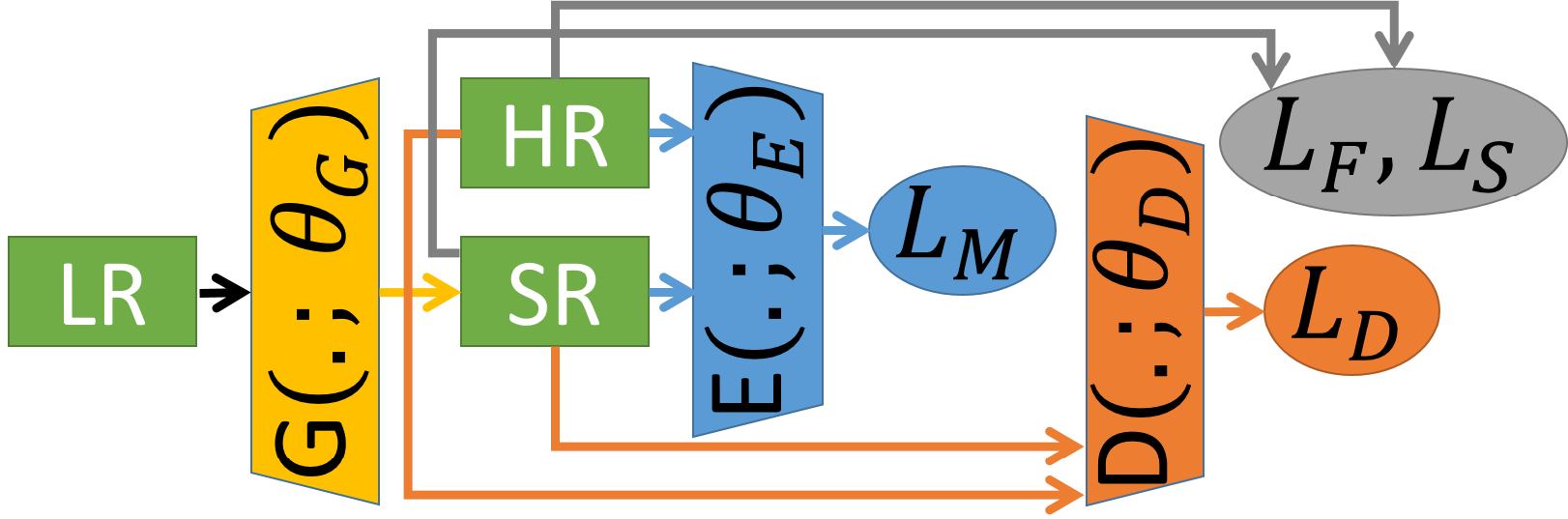
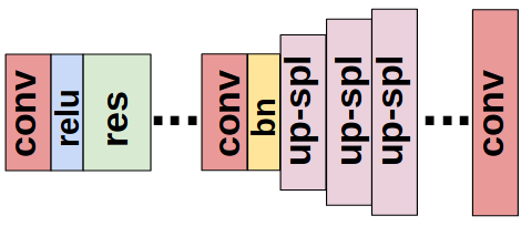
(a) Our SRGAN_SQE Architecture (b) Our Generator $\mathcal{G}(\cdot;\theta_{G})$

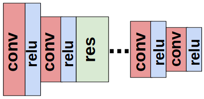
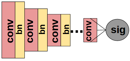
(c) Our Encoder $\mathcal{E}(\cdot;\theta_{E})$ (d) Our Discriminator $\mathcal{D}(\cdot;\theta_{D})$

Fig. 1: Our SRGAN_SQE Framework. (a) SRGAN_SQE framework along with the architectures of its underlying components: (b) generator, (c) encoder, (d) discriminator.

2.2 Our SRGAN_SQE Formulation and Training

Our SRGAN_SQE optimizes $\theta_{G}$, $\theta_{E}$, and $\theta_{D}$ using novel loss functions designed to (i) be robust to training-set corruptions and (ii) model realistic texture and human perception.

Robust Fidelity Loss. Typical GAN models penalize the MSE between the SR image $\mathcal{G}(X^{\text{LR}};\theta_{G})$ and the corresponding HR image $X^{\text{HR}}$. The MSE loss assumes the residual $\mathcal{G}(X^{\text{LR}};\theta_{G})-X^{\text{HR}}$ to have an isotropic Gaussian PDF, which can be incorrect because of training set corruptions due to errors in specimen preparation and staining, imaging artifacts, or human errors in dataset curation. For corrupted training sets, residual PDFs can have significantly heavier tails than a Gaussian, where the tails comprise examples that are clinically irrelevant. Such corruptions force the network to additionally learn mappings for LR-HR patch pairs that are very atypical, or even outliers, thereby risking a significant reduction in the performance of the network on patches that are actually clinically relevant for the application. Indeed, results in Section 3 support this claim. Thus, we propose to minimize the $q$-th power of the $q$-quasi-norm of the residual vector, where $q\in(0,1)$, thereby modeling the residual PDF as generalized Gaussian [13][14], with smaller $q$ leading to heavier tails. We make the loss function differentiable and usable in back-propagation, we use the $\epsilon$-regularised quasi norm. So, our novel robust fidelity loss is $\mathcal{L}_{F}(\theta_{G}):=E_{P(X^{\text{LR}},X^{\text{HR}})}[\|\mathcal{G}(X^{\text{LR}};\theta_{G})-X^{\text{HR}}\|_{q,\epsilon}^{q}]$ , where, for any image patch $a$ with pixel values $a_{i}$, we design $\|a\|_{q,\epsilon}^{q}:=\sum_{i}(|a_{i}|^{2}+\epsilon)^{q/2}$, with $\epsilon$ as small positive real found empirically. Our robust loss reweights of the MSE-based gradient that is proportional to the residual, such that gradients associated with larger residuals (e.g., caused by tail data or outliers) get scaled down for stable learning.

Robust Manifold-Based Loss. Our robust fidelity loss $\mathcal{L}_{F}$ enforces an independent pixelwise matching of the SR patch $\mathcal{G}(X^{\text{LR}};\theta_{G})$ with the corresponding HR patch $X^{\text{HR}}$. In addition, we also propose to penalize the dissimilarity in the underlying textural structures between $\mathcal{G}(X^{\text{LR}};\theta_{G})$ and $X^{\text{HR}}$, to capture the dependencies of pixel values across the entire patch. Hence, we propose a novel loss function that captures this dissimilarity by (pre-)learning the manifold representation of HR images through the encoder $\mathcal{E}(\cdot;\theta_{E})$ described in Section 2.1. In this manifold representation as well, the PDF of the residuals can be heavy tailed and, thus, we propose a novel robust loss relying on the manifold distance between SR patches and the corresponding HR patches: $\mathcal{L}_{M}(\theta_{G},\theta_{E}):=E_{P(X^{\text{LR}},X^{\text{HR}})}[\|\mathcal{E}(\mathcal{G}(X^{\text{LR}};\theta_{G});\theta_{E})-\mathcal{E}(X^{\text{HR}};\theta_{E})\|_{q,\epsilon}^{q}]$ .

Perception-Based Loss. In clinical applications, the SR image is interpreted by a human expert, e.g., a pathologist. Thus, we want SR patches to be perceptually identical to the (ground-truth) HR patches. During training, we propose to enforce human-perceptual similarity between the SR and HR patches by penalizing the negative sum of structural similarity (sSSIM) [15] values between SR and HR patches (sum taken over all overlapping $5\times 5$ neighborhoods in the SR and HR patches). We compute sSSIM on each of the three color channels (R,G,B) and add them up to give the overall sSSIM. This sSSIM accounts for perceptual changes in structural information, luminance, and contrast over all neighborhoods between the SR and HR patches. Thus, we propose the perception-based loss as $\mathcal{L}_{S}(\theta_{G}):=-E_{P(X^{\text{LR}},X^{\text{HR}})}[\text{sSSIM}(\mathcal{G}(X^{\text{LR}};\theta_{G}),X^{\text{HR}})]$ .

Discriminator Loss. Our discriminator training penalizes the Kullback-Leibler (KL) divergences between (i) the probability vectors (distributions) for the SR and HR patches produced by the discriminator, i.e., $[\mathcal{D}(\mathcal{G}(X^{\text{LR}};\theta_{G});\theta_{D}),1-\mathcal{D}(\mathcal{G}(X^{\text{LR}};\theta_{G});\theta_{D})]$ or $[\mathcal{D}(X^{\text{HR}};\theta_{D}),1-\mathcal{D}(X^{\text{HR}};\theta_{D})]$, and (ii) the one-hot probability vectors (distributions) for the SR and HR patches, i.e., $[0,1]$ or $[1,0]$, respectively. Thus, our discriminator-based loss function is $\mathcal{L}_{D}(\theta_{G},\theta_{D}):=E_{P(X^{\text{LR}},X^{\text{HR}})}[\log(1-\mathcal{D}(\mathcal{G}(X^{\text{LR}};\theta_{G});\theta_{D}))+\log(\mathcal{D}(X^{\text{HR}};\theta_{D}))]$ . On one hand, the generator optimizes $\theta_{G}$ to reduce the loss function $\mathcal{L}_{D}$, where the generator learns to produce high-quality SR patches $\mathcal{G}(X^{\text{LR}};\theta_{G})$ that “trick” the discriminator in assigning them a high probability $\mathcal{D}(\mathcal{G}(X^{\text{LR}};\theta_{G});\theta_{D})$ of being in the HR class, i.e., being drawn from $P(X^{\text{HR}})$. On the other hand, the discriminator training optimizes $\theta_{D}$ to increase the “gain” function $\mathcal{L}_{D}$, where the discriminator learns to give (i) HR patches high probabilities $\mathcal{D}(X^{\text{HR}};\theta_{D})$ of belonging to the HR class and (ii) SR patches low probabilities $\mathcal{D}(\mathcal{G}(X^{\text{LR}};\theta_{G});\theta_{D})$ of belonging to the HR class.

SRGAN_SQE Formulation and Training. We train our SRGAN_SQE to optimize the parameters $\theta_{G},\theta_{D}$ by solving $\arg\min_{\theta_{G}}\arg\max_{\theta_{D}}[\mathcal{L}_{F}(\theta_{G})+\lambda_{M}\mathcal{L}_{M}(\theta_{G},\theta_{E})+\lambda_{S}\mathcal{L}_{S}(\theta_{G})+\lambda_{D}\mathcal{L}_{D}(\theta_{G},\theta_{D})]$, where $\lambda_{M},\lambda_{S},\lambda_{D}$ are positive real free parameters that control the balance across the loss functions. In this paper, $\lambda_{M}:=0.2$, $\lambda_{S}:=2$, $\lambda_{D}:=0.016$. We use alternating optimization on $\theta_{G}$ and $\theta_{D}$, using back-propagation and Adam optimizer [16] (for all $q$). We train the generator using the non-saturating heuristic [17].

3 Results and Discussion

We evaluate using histopathology images from the CAMELYON dataset [18]. We extract 4000 patches of size $256\times 256$ pixels at the highest resolution and consider them as HR ground truth. We Gaussian-smooth and subsample HR patches to create LR patches ($64\times 64$ pixels). We use 2000 patches for training and 2000 for testing. We evaluate four methods: (i) SRGAN [8], a current state of the art; (ii) our SRGAN_E, where $q:=2,\lambda_{S}:=0$; (iii) our SRGAN_QE, where $q\in(0,1),\lambda_{S}:=0$; (iv) our SRGAN_SQE, where $q\in(0,1),\lambda_{S}>0$. We evaluate performance using three quantitative measures: (i) relative root MSE (RRMSE) between SR and HR images, i.e., $\|\mathcal{G}(X^{\text{LR}};\theta_{G})-X^{\text{HR}}\|_{\text{F}}/\|X^{\text{HR}}\|_{\text{F}}$, (ii) multiscale mean SSIM (MS-mSSIM) that averages SSIM across neighborhoods at five different scales [15], (iii) quality index based on local variance (QILV) [19]. While MS-mSSIM is more sensitive to random noise than blur in the images, QILV acts complementarily and is more sensitive to blur than noise.

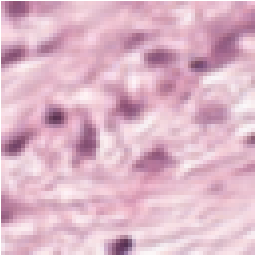
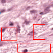
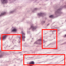
(a1) Low-res. (b1) Ground truth (c1) SRGAN

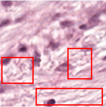
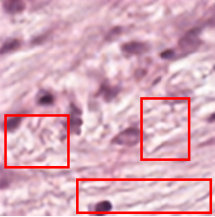
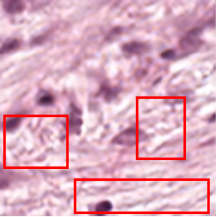
(d1) SRGAN_E (e1) SRGAN_QE (f1) SRGAN_SQE

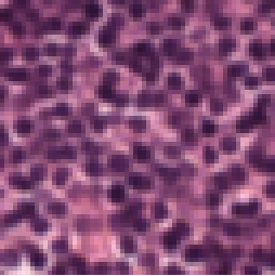
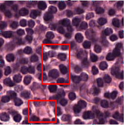
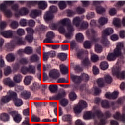
(a2) Low-res. (b2) Ground truth (c2) SRGAN

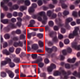
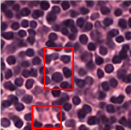
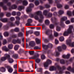
(d2) SRGAN_E (e2) SRGAN_QE (f2) SRGAN_SQE

Fig. 2: Results without Explicitly Corrupting Training Set. (a1)-(a2) LR input. (b1)-(b2) HR ground truth. [MS-mSSIM,RRMSE,QILV] for (c1)-(c2) SRGAN: [0.67,0.004,0.973], [0.87,0.14,0.972]; (d1)-(d2) SRGAN_E: [0.86,0.001,0.975], [0.87,0.011,0.973]; (e1)-(e2) SRGAN_QE: [0.89,0.001,0.987], [0.89,0.007,0.984]; (f1)-(f2) SRGAN_SQE: [0.91,0.001,0.996], [0.90,0.008,0.993].

We start by evaluating methods on our training set that is well curated and does not contain any explicitly-introduced corrupted examples. The training data exhibit natural variability in terms of texture, contrast, intensity histograms, and focus. First, replacing the VGG-encoding in SRGAN (Figure 2(c1)-(c2)) with our (pre-)learned autoencoder-based encoding $\mathcal{E}(\cdot;\theta_{E})$ and manifold-based loss $\mathcal{L}_{M}$ in SRGAN_E improves the results qualitatively (Figure 2(d1)-(d2)) and quantitatively (Figure 3(a1)–(a3)). Second, with $q<1$, our SRGAN_QE (Figure 2(e1)-(e2)), improves over SRGAN_E, indicating that the distribution of residuals (in spatial and encoded domains) even with natural variability is much heavier tailed than Gaussian (best results for $q\approx 0.5$). The improvement is evident quantitatively in Figure 3(a1)–(a3) when fraction of corrupted examples is zero. Our perceptual sSSIM-based loss $\mathcal{L}_{S}$, even at a single scale of $5\times 5$ pixel neighborhoods, in our SRGAN_SQE leads to further improvements, when our SR images (Figure 2(f1)-(f2)) become virtually identical to the HR image qualitatively (Figure 2(b1)-(b2)) and quantitatively (Figure 3(a1)–(a3)).

Next, we evaluate all methods by explicitly introducing corrupted examples during training, in the form of increasing levels of noise (e.g., from weak signals), blur (e.g., from poor focus), or changes in contrast (e.g., from poor staining). Quantitatively, our SRGAN_SQE outperforms all other methods, for varying levels of corruption from 0% to 50% (Figure 3(a1)–(a3)). Modeling heavy-tailed residuals with $q\approx 0.5$ gives the best results across all measures (Figure 3(b1)–(b3)). As the level of corruptions increase from 5% to 30%, the results from our SRGAN_SQE (Figure 4(c1)-(c2)) stay stable and high-quality, visually and quantitatively, but the results from SRGAN (Figure 4(d1)-(d2)) degrade significantly.

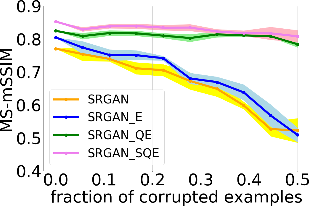
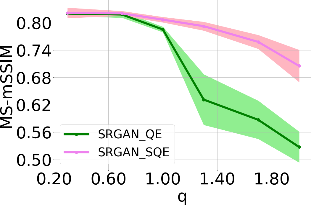
(a1) (b1)

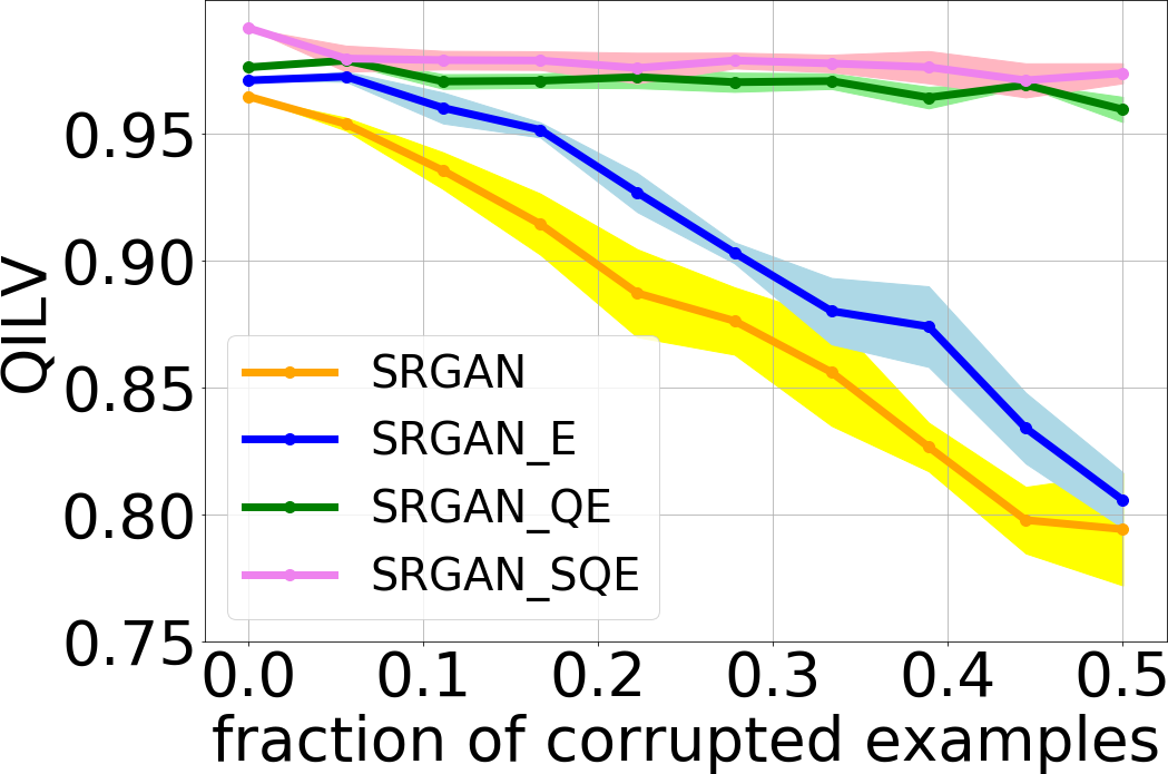
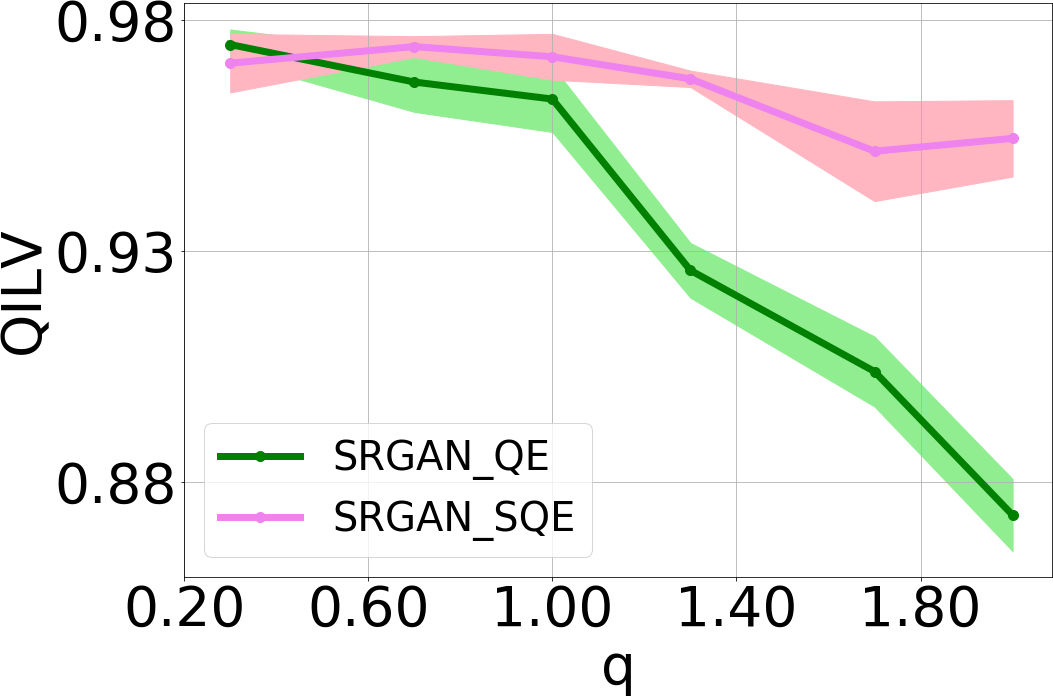
(a3) (b3)

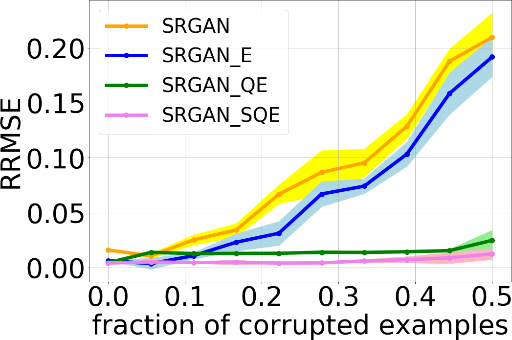
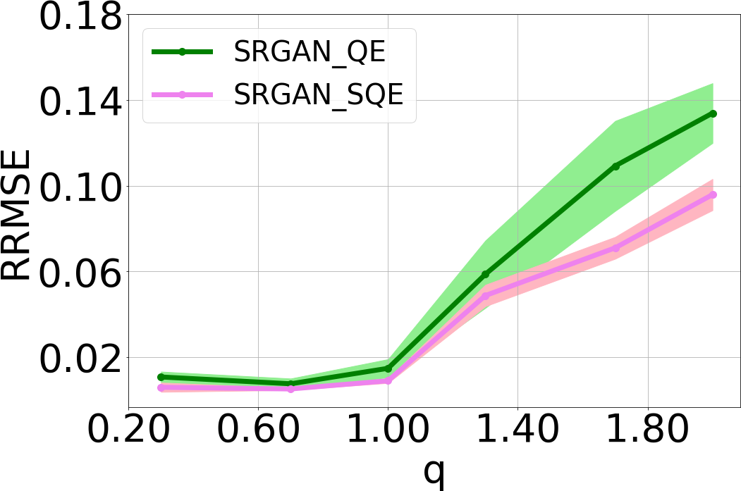
(a2) (b2)

Fig. 3: Results with Varying Levels of Training-set Corruption and Robustness $q$. Plots for MS-mSSIM, QILV, and RRMSE for: (a1)–(a3) varying fractions of corrupted examples introduced in training set ($q$=0.5); (b1)–(b3) varying robustness $q$ (corrupted fraction in training dataset =$0.3$).

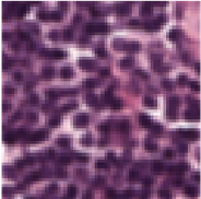
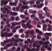
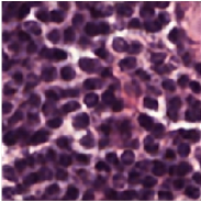
(a) Low-res. input (c1) SRGAN_SQE (d1) SRGAN

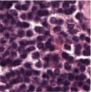
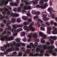
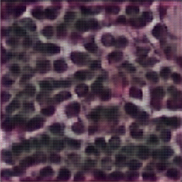
(b) Ground truth (c2) SRGAN_SQE (d2) SRGAN

Fig. 4: Results with Varying Levels of Training-set Corruption. (a) LR input. (b) HR ground truth. Results for (c1)-(c2) Our SRGAN_SQE and (d1)-(d2) SRGAN, with $5\%$ and $30\%$ corrupted examples introduced in the training set. [MS-mSSIM,RRMSE,QILV] for: (c1)-(c2) Our SRGAN_SQE are [0.91,0.01,0.993] and [0.91,0.01,0.987]; (d1)-(d2) SRGAN are [0.85,0.02,0.976] and [0.76,0.15,0.853].

Conclusion. We proposed the novel SRGAN_SQE framework for super-resolution that makes learning robust to errors in training-set curation by modeling heavy-tailed PDFs, using quasi norms, on the residuals in the spatial and manifold-encoding domains. We learned the manifold, using an autoencoder, to reproduce realistic textural details. We proposed a sSSIM based loss, at a single fine scale, to output SR images matching human perception. Results on a large clinical dataset showed that our SRGAN_SQE improves the quality of the super-resolved images over the state of the art quantitatively and qualitatively.

References

- [1] Hong Chang, Dit-Yan Yeung, and Yimin Xiong, “Super-resolution through neighbor embedding,” in IEEE Conference on Computer Vision and Pattern Recognition (CVPR), 2004, pp. 275–82.
- [2] J Yang, J Wright, T Huang, and Y Ma, “Image super-resolution via sparse representation,” IEEE Transactions on Image Processing (TIP), vol. 19, no. 11, pp. 2861–73, 2010.
- [3] H Mousavi and V Monga, “Sparsity-based color image super resolution via exploiting cross channel constraints,” IEEE Transactions on Image Processing (TIP), vol. 26, no. 11, pp. 5094–106, 2017.
- [4] Samuel Schulter, Christian Leistner, and Horst Bischof, “Fast and accurate image upscaling with super-resolution forests,” in IEEE Conference on Computer Vision and Pattern Recognition (CVPR), 2015, pp. 3791–9.
- [5] Chao Dong, Chen Change Loy, Kaiming He, and Xiaoou Tang, “Learning a deep convolutional network for image super-resolution,” in European Conference on Computer Vision (ECCV), 2014, pp. 184–99.
- [6] Joan Bruna, Pablo Sprechmann, and Yann LeCun, “Super-resolution with deep convolutional sufficient statistics,” in International Conference on Learning Representations (ICLR), 2016, pp. 1–17.
- [7] Wei-Sheng Lai, Jia-Bin Huang, Narendra Ahuja, and Ming-Hsuan Yang, “Deep Laplacian pyramid networks for fast and accurate superresolution,” in IEEE Conference on Computer Vision and Pattern Recognition (CVPR), 2017, pp. 5835–5843.
- [8] Christian Ledig, Lucas Theis, Ferenc Huszár, Jose Caballero, Andrew Cunningham, Alejandro Acosta, Andrew Aitken, Alykhan Tejani, Johannes Totz, Zehan Wang, and Wenzhe Shi, “Photo-realistic single image super-resolution using a generative adversarial network,” in IEEE Conference on Computer Vision and Pattern Recognition (CVPR), 2017, pp. 105–114.
- [9] Karen Simonyan and Andrew Zisserman, “Very deep convolutional networks for large-scale image recognition,” in International Conference on Learning Representations (ICLR), 2015.
- [10] Y. Lecun, L. Bottou, Y. Bengio, and P. Haffner, “Gradient based learning applied to document recognition,” in Proceedings of the IEEE, 1988, pp. 2278–2324.
- [11] Christian Szegedy Sergey Ioffe, “Batch normalization: Accelerating deep network training by reducing internal covariate shift,” in International Conference on Machine Learning (ICML), 2015, pp. 448–456.
- [12] P Baldi, “Autoencoders, unsupervised learning, and deep architectures,” in Proc. International Conference on Machine Learning (ICML) Workshop on Unsupervised and Transfer Learning, 2012, pp. 37–49.
- [13] M Novey, T Adali, and A Roy, “A complex generalized Gaussian distribution-characterization, generation, and estimation,” IEEE Transactions on Signal Processing (TSP), vol. 58, no. 3, pp. 1427–33, 2010.
- [14] M. P. Shah, S. N. Merchant, and S. P. Awate, “Abnormality detection using deep neural networks with robust quasi-norm autoencoding and semi-supervised learning,” in 2018 IEEE 15th International Symposium on Biomedical Imaging (ISBI 2018), 2018, pp. 568–572.
- [15] Zhou Wang, A.C. Bovik, H.R. Sheikh, and E.P. Simoncelli, “Image quality assessment: From error visibility to structural similarity,” IEEE Transactions on Image Processing (TIP), vol. 13, no. 4, pp. 600–612, 2004.
- [16] Diederik P. Kingma and Jimmy Ba, “Adam: A method for stochastic optimization,” in International Conference on Learning Representations (ICLR), 2015.
- [17] Ian J. Goodfellow, Jean Pouget-Abadie, Mehdi Mirza, Bing Xu, David Warde-Farley, Sherjil Ozair, Aaron Courville, and Yoshua Bengio, “Generative adversarial nets,” in Advances in Neural Information Processing Systems (NIPS), 2014, pp. 2672–80.
- [18] “Camelyon-16,” https://camelyon16.grand-challenge.org, 2016.
- [19] Aja-Fernández, Estépar RS, Alberola-López C, and Westin CF., “Image quality assessment based on local variance,” in IEEE EMBS Annual International Conference, 2006, pp. 4815–8.