Adaptive image processing: a bilevel structure learning approach for mixed-order total variation regularizers
Abstract.
A class of mixed-order PDE-constraint regularizer for image processing problem is proposed, generalizing the standard first order total variation . A semi-supervised (bilevel) training scheme, which provides a simultaneous optimization with respect to parameters and new class of regularizers, is studied. Also, A finite approximation method, which used to solve the global optimization solutions of such training scheme, is introduced and analyzed.
Key words and phrases:
image processing, optimal training scheme, higher order differential operators, -convergence2010 Mathematics Subject Classification:
26B30, 94A08, 47J201. Introduction
The use of variational technics with non-smooth regularizers in image processing has become popular in the last decades. One of the most successful approaches is introduced in the celebrated work [20] which relies on the so called ROF total-variational functional
| (1.1) |
where is a given corrupted image, represents the unit square, is an intensity parameter, and stands for the total variation of in (see [14]). In the simple case that , we have
| (1.2) |
One advantage of using the regularization is it promotes piecewise constant reconstructions, thus preserving edges. However, this also leads to blocky-like artifacts in the reconstructed image, an effect known as stair-casing. To mitigate this effect, and also to explore possible improvements, the following methods has been introduced and studied:
- 1.
-
2.
changing the underlying Euclidean norm ([22]);
- 3.
These methods introduces collections of regularizers which generalizes seminorm. For example, in [22], the underlying Euclidean norm of seminorm is generalized from , used in (1.2), to by
| (1.3) |
In [18], the order of derivative is generalized from , used in (1.2), to , by
| (1.4) |
in which the fractional order derivative is realized by using the Riemann-Liouville fractional order derivative (see [21] for definition). In both [18, 10], it has been shown that for given corrupted image , a carefully selected regularizer parameter (resp. ) allows (resp. ) to provide improved imaging processing result, and such selection can be done automatically by using a bi-level training scheme which will be detailed below.
In general, with a reliable selection mechanism, the imaging processing results would certainly be improved if we could further expand the collections of regularizers. To this purpose, in this paper we introduce a family of novel -like PDE-constraint regularizer (semi-norm), say , by
| (1.5) |
Here denotes the Radon norm of a measure, and : is a linear differential operator (see Notation 2.1).
In the simple case , we recover the total variation seminorm. We remark that the abstract framework studied in (1.5) naturally incorporates the recent PDE-based approach to image denoising problems formulated in [1], and also allows us to simultaneously describe a variety of different image-processing techniques.
The aim of this paper is threefold. First, we provide a rigorous and detailed analysis of the properties of the seminorm, such as the approximation by smooth functions,
lower semi-continuity with respect to both function and operator , and a point-wise characterization of the sub-gradient of .
The second result is the study of the aforementioned selection mechanism, realized by a semi-supervised (bilevel) training scheme
defined in machine learning (see [7, 8, 12, 23, 11, 17]).
For example, we could apply the bilevel training scheme to determine the optimal value of from (1.1), which controls the strength of the regularizer.
More precisely, we assume that the corrupted image can be decomposed as where represents a noise-free clean image (the perfect data), and encodes noise, and we call as training set. Then, a bilevel training scheme, say Scheme , for determining the optimal intensity parameter can be formulated as follows:
| Level 1. | (-L1) | |||
| Level 2. | (-L2) |
where , used in (-L1), is called the training ground. Roughly speaking, Level 1 problem in (-L1) looks for an that solves the minimum -distance to the clean image , subject to the minimizing problem (-L2). That is, scheme is able to optimally adapt itself to the given “perfect data” .
In the same spirit, in order to identify the optimal operator in for a given training set , we introduce the scheme ((-L1)-(-L2)) defined as
| Level 1. | (-L1) | |||
| Level 2. | (-L2) |
In (-L1), we expand the training ground to to incorporate the new parameter , where denotes a closed collection of operators (see Notation 2.1, Notation 4.1, and (4.5) for details). We remark that the expanded training ground allows scheme to optimize the regularizer and intensity parameter simultaneously. We summarize the main result in the following theorem.
Theorem 1.1 (see Theorem 4.4).
The training scheme admits at least one solution , and provides an associated optimally reconstructed image .
In the third part of this article we focus on how to numerically determine the optimal solution of scheme , or equivalently, compute global minimizers of the assessment function : defined as
| (1.6) |
where is obtained from (-L2). However, as shown in [22] that even in the simplest case with (i.e. ), the assessment function is not quasi-convex (in the sense of [16], or simply convex), and hence the methods such as Newton’s descent or Line search might get trapped in a local minimum. To overcome this difficulty, we introduce the concept of the acceptable optimal solution. To be precise, we say the solution is an acceptable optimal solution of scheme with the given error if
| (1.7) |
where is a global minimum obtained from (-L1).
To compute such acceptable optimal solution,
we use a finite approximation method, originally introduced and studied in [22], and generalized in Section 4.2
to fit our new regularizer . To this aim, and also for the numerical realization of scheme , we add the following box-constraint on the training ground .
-
•
The intensity parameter is contained in a closet interval , where the box-constraint constant can be chosen by the user;
-
•
the collection of operator satisfies an additional continuity assumptions, such as, for any , ,
(1.8) where denotes the big- notation.
Then, the finite approximation method is constructed based on a sequence of (finite) training sets , indexed by , in which (where denotes the counting measure)
| (1.9) |
For the precise definition of we refer readers to Definition 4.7. We remark that, since for each fixed, we could evaluate at each element of and determine the optimal solution(s)
| (1.10) |
precisely. The following theorem is established in order to achieve (1.7).
Theorem 1.2 (see Theorem 4.9).
Let a training ground satisfies above box-constraint. Then the following assertions hold:
-
1.
we have
(1.11) -
2.
Let be given. Then for each we have
(1.12) where the value of right hand side can be computed explicitly.
That is, for any given , we could compute that is large enough so that the corresponding optimal solution is
an acceptable optimal solution of scheme . Also, in Section 5.1 we show that, even with the box-constraint, the training ground is still sufficiently large to
encompass interesting operator. We finally remark that, although this work focuses mainly on the theoretical analysis of the operators and the training scheme , in Section 5.1 a primal-dual algorithm for solving (-L2) is discussed, and some preliminary numerical demonstration of scheme are provided.
Our article is organized as follows. In Section 2 we analyze the functional properties of the -seminorms.
The -convergence result, the bilevel training scheme, and the finite approximation are the subjects of Sections 3 and 4, respectively.
Finally, in Section 5.1 we demonstrate several numerical implementations, and in Section 5.2 some possible extensions of .
2. The space of functions with bounded -seminorm
Let , be given, and let be the unit open cube in . is the space of matrices with dimension ( times) with elements in . For the convenience of the presentation of this article, we identify the matrix space by vector space , where ( times). Moreover, represents the space of distributions with values in .
Notation 2.1.
We collect some notation which will be adopted in connection with linear differential operators.
-
1.
For , we let : , denote the -th Hessian differential operator. For example, when we have ;
-
2.
For each , we let be matrix mapping from to and
(2.1) We denote by : the -th order differential operator
(2.2) -
3.
For each , we denote the formal adjoint of the matrix by , and we define the differential operator : by
(2.3) -
4.
We denote the bilinear operator , induced by , such that
(2.4) -
5.
Given a sequence of operators and an operator , with coefficients and , respectively, we say that in if
(2.5) where stands for the matrix norm.
Definition 2.2.
Let be fixed. We denote by the collection of operator defined in notation 2.1, with order at most .
2.1. The PDE-constraint total variation defined by operator
We generalize the standard total variation seminorm by using the -th order differential operators defined in Definition 2.2.
Definition 2.3.
Let and operator be given.
-
1.
We define the PDE-constraint seminorm, say , by
(2.6) -
2.
We define the space
(2.7) and we equip it with the norm
(2.8)
In next proposition we collect several preliminary results regarding functions in space .
Proposition 2.4.
Let operator and be given.
-
1.
For any sequence and function that satisfying one of the following conditions:
-
i.
is locally uniformly integrable and a.e..
-
ii.
in .
Then, we have
(2.9) -
i.
-
2.
There exists a Radon measure and a -measurable function : such that
-
i.
-a.e.;
-
ii.
for all , there holds
(2.10)
-
i.
Proof.
We prove Assertion 1 first. If
| (2.11) |
there is nothing to prove. Assume not, then we have, for arbitrary , that
| (2.12) |
where the last equality can be deduced either from condition 1(i) or 1(ii), independently. Hence, we conclude (2.9) in view of the arbitrariness of .
We next prove Assertion 2. We define the linear functional : such that
| (2.13) |
Then, since , we have that
| (2.14) |
which implies that
| (2.15) |
Now, for arbitrary , we define the mollifications , for some mollifier with . Then we have, by [14, Theorem 1, item (ii), Section 4.2], that uniformly on . Therefore, by defining
| (2.16) |
and together with (2.15), we conclude that
| (2.17) |
Thus, in view of the Riesz representation theorem (see [14, Section 1.8]), the proof is complete. ∎
Remark 2.5.
We henceforth write by and have
| (2.18) |
for arbitrary .
Theorem 2.6 (local approximation by smooth functions).
Let and be given. There exists a sequence such that the following assertions hold.
-
1.
strongly in ;
-
2.
.
-
3.
for each .
Remark. Assertion 3 only asserts that for each fixed that but it is possible that as . In another word, we make no conclusions with respect to the trace value of from Theorem 2.6.
Proof.
The construction of approximation sequence is almost same to the approximation sequence used in the standard case as presented in [14, Theorem 2, Page 172]. We shall only concentrated on showing that Assertion 3 holds, but for reader’s convenience, we shall outline the construction of approximation sequence and key steps.
Let be given, and let be the cube centered at point with side length . Let arbitrary be given, we choose large enough such that
| (2.19) |
Define and
| (2.20) |
Let be the partition of unity such that
| (2.21) | |||
| (2.22) |
Let be the standard mollifier, and for each , we choose small enough such that
| (2.23) | |||
| (2.24) | |||
| (2.25) |
and we define
| (2.26) |
We observe that (2.23) implies that , and (2.24) implies that
| (2.27) |
This, and together with Assertion 1, Proposition 2.4, we conclude that
| (2.28) |
Next, for arbitrary , we observe that,
| (2.29) |
where at the first equality we used the linearity of convolution operator, and at the last equality we used (2.4). Thus, we have
| (2.30) |
Following the same computation used in [14, Theorem 2, Page 172] and use (2.25), we deduce that
| (2.31) |
Hence, in view of the arbitrariness of , we obtain that
| (2.32) |
Lastly, we further modify the sequence so that for each . Let be given and we define
| (2.33) |
Consequentially, we have in strong and , as . Hence, by using a diagonal argument, we could extract a subsequence such that
| (2.34) |
On the other hand, by the definition of , we have , which concludes Assertion 3 as desired. ∎
Remark. The construction of in (2.33) is possible because of the simple geometry of domain . However, for domain with arbitrary geometry, even with Lipschitz boundary, such construction is not available. We refer readers to [4, 15] for alternative constructions with, however, operator with several additional restriction.
Corollary 2.7.
Let a finite set of , , be given and
| (2.35) |
Then, there exists a sequence
| (2.36) |
such that the following assertions hold.
-
1.
strongly in ;
-
2.
, for each uniformly;
-
3.
for each .
Proof.
We close this section by stating the l.s.c. result of semi-norm.
Proposition 2.8.
Let and sequence such that in be given. Then, we have that
| (2.38) |
Proof.
First of all, if
| (2.39) |
then there is nothing to prove. Suppose
| (2.40) |
then, for arbitrary , we have that
| (2.41) |
Hence, by taking supremum with respect to on the right hand side of above inequality, we conclude that
| (2.42) |
as desired. ∎
3. Analytic properties of PDE-constraint variations
3.1. -convergence of functionals defined by seminorms
In this section we prove a -convergence result with respect to the intensity parameter and operator .
Definition 3.1.
We define the functional : as
| (3.1) |
The following theorem is the main result of this section.
Theorem 3.2.
Let sequences and be given such that in and . Then, the functional -converges to in the weak topology. To be precise, for every the following two conditions hold:
(Lower semi-continuity) If
| (3.2) |
then
| (3.3) |
(Recovery sequence) For each , there exists such that
| (3.4) |
and
| (3.5) |
We subdivide the proof of Theorem 3.2 into two propositions.
The following proposition is instrumental for establishing the liminf inequality.
Proposition 3.3.
Let sequences and be given such that in and . Let be given such that there exists and
| (3.6) |
Then there exists such that, up to the extraction of a subsequence (not relabeled),
| (3.7) |
and
| (3.8) |
Proof.
Without loss of generality we assume that for every , as the general case for and can be argued with straightforward adaptations.
From (3.6) and the fact we have, up to a subsequence, that there exists such that (3.7) holds.
Next, for arbitrary , we observe that
| (3.9) | ||||
| (3.10) |
where at the last we used the fact that and the Lebesgue dominated convergence theorem.
Hence, we could obtain that
| (3.11) | |||
| (3.12) |
where at the last inequality we used (3.7) and (3.9). Thus, by the arbitrarness of , we conclude (3.8), and hence the thesis. ∎
Proposition 3.4 (- inequality).
Let sequences and be given such that in and . Then, for every there exist and, up to a subsequence of , such that in and
| (3.13) |
Proof.
If , there is nothing to prove. Suppose not, and assume for a moment that , which indicates that for each . Fix , and chose such that
| (3.14) |
We observe that
| (3.15) |
where at the last inequality we used the fact that satisfies (2.8). Next, since and in , we have
| (3.16) |
which implies that
| (3.17) |
Thus, we could apply the Lebesgure dominate convergence theorem to conclude that
| (3.18) |
This, and together with (3.14) and (3.15), we observe that
| (3.19) |
which implies, by sending second, that
| (3.20) |
Next, by Theorem 2.6, we could construct an approximation sequence such that in and
| (3.21) |
Also, by (3.20), we have
| (3.22) |
Thus, by a diagonal argument, we can obtain a sequence such that
| (3.23) |
That is, we have
| (3.24) |
which concludes our thesis. ∎
3.2. The point-wise characterization of sub-differental of
We recall few notations and preliminary results and definitions first.
Definition 3.5 ([13, Definition 4.1 & 5.1]).
Let be a function of normed space into be given.
-
1.
We define the polar function of , denoted by , by
(3.25) -
2.
We define the bipolar function, say , of by
(3.26) -
3.
We say is sub-differentiable at point if is finite and there exists such that
(3.27) for all . Then we call such is called a sub-gradient of at , and the set of sub-gradients at is called the sub-differential at and is denoted .
Proposition 3.6 ([13, Proposition 4.1 & 5.1]).
Let be a function of into and its polar. Then the following assertions hold.
-
1.
We have if and only if
(3.28) -
2.
The set (possible empty) is convex and closed.
-
3.
If in addition is convex, then .
Definition 3.7.
Let , , and operator be given.
-
1.
we say that in if there exists such that for all
(3.29) -
2.
we define the space
(3.30) with the norm
(3.31) -
3.
we define
(3.32) i.e., the closure of function space with respect to norm.
-
4.
we define
(3.33) and
(3.34)
The main result of Section 3.2 reads as follows.
Theorem 3.8.
Let , , and , . Then if and only if
-
1.
;
-
2.
there exist such that , , and
(3.35)
We prove Theorem 3.8 in several propositions.
Proposition 3.9.
Let be given. Then we have the closure of function space under norm equals to the function space , i.e.,
| (3.36) |
Proof.
We claim
| (3.37) |
first, and we do it by showing the space is closed with respect to norm. Let be given, and extract a sequence such that
| (3.38) |
Since , we have and hence, up to a subsequence, there exists such that
| (3.39) |
Next, let be given, and we observe that
| (3.40) |
and together with (3.38), we have
| (3.41) |
which implies that . Thus, we have . Next, since the set
| (3.42) |
is convex and closed, hence by [5, Theorem 3.7], it is weakly closed. Thus, we conclude that , which implies that , or the function space is closed with respect to norm, which also conclude (3.37) as desired.
We next claim that
| (3.43) |
We prove (3.43) by following arguments used in [14, Theorem 2, Page 125]. Let be given. That is, there exists , , and . From the definition of , there exists such that
| (3.44) |
Next, define the truncation function
| (3.45) |
and we note that
| (3.46) |
Using a similar argument used in Proposition 2.4, and together with a.e., we obatin that
| (3.47) |
On the order hand, by (3.45), we have
| (3.48) |
and hence
| (3.49) |
This, and together with the second part in (3.46), and using [5, Exercise 4.19, 1, page 124], we conclude that
| (3.50) |
We next modify the sequence so that . We obtain sequence of sets , , and partition of unity from the argument used in Theorem 2.6. Next, for each , we choose small enough such that
| (3.51) | |||
| (3.52) | |||
| (3.53) |
and in addition, we choose small that
| (3.54) |
Then, we define
| (3.55) |
and (3.54) indicates that . Following the same calculation in [14, Theorem 2, Page 125], we have that
| (3.56) |
together with (3.44), and a diagonal argument, we could construct a sequence such that
| (3.57) |
Moreover, we observe that
| (3.58) |
which proves that , and hence (3.43), and our thesis. ∎
Now we ready to prove Theorem 3.8.
Proof of Theorem 3.8.
We first claim that the convex conjugate of , say , has the form that
| (3.59) |
By Definition 3.5 and Proposition 3.9, we have that
| (3.60) |
Next, since the seminorm and indictor function are convex and lower semi-continuity, we have
| (3.61) |
Finally, in view of Proposition 3.6, we have that
| (3.62) |
if and only if
| (3.63) |
and we are done. ∎
Remark 3.10.
Theorem 3.11 (The point-wise characterization of ).
Let , , be given. Let such that . Then we have
| (3.65) |
where is the density of with respect to (see Remark 2.5).
Proof.
Let be given and be obtained from Theorem 3.8. Then, by the definition of , we could obtain a sequence such that strongly in .
We claim that
| (3.66) |
From the definition of and Theorem 2.5, we have that
| (3.67) |
On the order hand, since , we have and hence, together with the fact that a.e., we observe that
| (3.68) | ||||
| (3.69) |
Therefore, we could compute that
| (3.70) | ||||
| (3.71) | ||||
| (3.72) |
Next, from (3.67), we have that
| (3.73) |
This, and together with (3.70), we conclude (3.66) as desired. ∎
Proposition 3.12.
Let and be given. Let and , then we have
| (3.74) |
Proof.
We obtain and such that Assertions 1 and 2 hold for and , respectively. Then, by Theorem 3.11 we have both and can be represented point-wisely by the density of with respect to , and we are done. ∎
4. Learning the optimal operator in imaging processing problems
In this section we use the bilevel training scheme introduced in Section 1 to determine the optimal setting of for a given training pairs , where and represents the corrupted and clean image, respectively.
4.1. The bilevel training scheme with the regularizer
We collect few notations first.
Notation 4.1.
Recall the definition of from Notation 2.1.
-
1.
We denote by the collection of operators such that
(4.1) -
2.
We denote the TrainingGround by
(4.2)
We state below the definition of training scheme and associated notations.
Definition 4.2.
We define the training scheme with underlying training ground by
| Level 1. | (-L1) | |||
| Level 2. | (-L2) |
In particular, for the case that , we define
| (4.3) |
In (-L1), we denote by notation the collection of optimal solution(s) of scheme with underlying training ground , and is an optimal solution obtained from training ground .
We first show that the Level 2 problem (-L2) admits a unique solution.
Proposition 4.3.
Let and be given. Then, there exists a unique such that
| (4.4) |
Proof.
The proof can be obtained by Proposition 2.8 and the fact that is convex. ∎
Theorem 4.4.
Let the training ground be given. Then the training scheme admits at least one solution , and provides an associated optimally reconstructed image .
Proof.
Let be a minimizing sequence obtained from (-L1). Then, by the boundedness and closedness of in , up to a subsequence (not relabeled), there exists such that in , in , and
| (4.5) |
We divide our arguments into three cases.
Case 1: Assume . Then, in view of Theorem 3.2 and the properties of -convergence, we have
| (4.6) |
where and are obtained from (-L2). Thus, we deduce that
| (4.7) |
which completes the thesis.
Case 2: Assume . Then by (4.5), up to a subsequence, there exists such that weakly in . We claim that in strong. Extend by zero outside and we define
| (4.8) |
where is the standard mollifier. Then we have and strongly in . By the optimality condition of (-L2), we have
| (4.9) | |||
| (4.10) |
That is, we have
| (4.11) |
and we are done by letting first and second.
Case 3: Assume . Reasoning as in Case 2, we have again that there exists such that
| (4.12) |
Then, in this case we have, by (4.3), that
| (4.13) |
as desired. ∎
4.2. Numerical realization and finite approximation of scheme
For the numerical realization of training scheme , we in addition require that the training ground satisfies the following assumption.
Assumption 4.5.
Let the order be given.
- 1.
-
2.
We assume the collection of operator satisfies the following two conditions.
-
a.
Each operator has at most order (the box-constraint on order of );
-
b.
For any , , the continuity assumption
(4.14) and
(4.15) holds.
-
a.
The following corollary is a direct consequence of Theorem 4.4
Corollary 4.6.
The training scheme , with a underlying training ground satisfies Assumption (4.5), admits at least one solution , and provides an associated optimally reconstructed image .
Proof.
The argument is identical to the argument used in Theorem 4.4, Case 1 & Case 2. ∎
Recall the definition of the assessment operator from (1.6) that
| (4.16) |
As discussed in Section 1, the Level 1 problem (-L1) for scheme is equivalent to find global minimizers of among the training ground . However, in view of the counter-example provided in [22], the assessment function is not convex, and hence the traditional methods like Newton’s descent or Line search could trapped into local minimums, but not convergence to global minimums.
We overcome this problem by using a finite approximation method original introduced in [22]. Recall the constant given in box-constraint stated in Assumption 4.5.
Definition 4.7 (The Finite TrainingGround and Finite Grid).
Let be given.
-
1.
We define the step size by
(4.17) -
2.
we define the finite set via
(4.18) -
3.
we define the finite set via
(4.19) where each is a singleton contains one operator and defined recursively in the following steps.
-
Step 1.
Define
(4.20) We also denote be the cube centered at with side length .
-
Step 2.
Define
(4.21) and
(4.22) -
Step .
Define
(4.23) and
(4.24) Repeat until .
-
Step 1.
-
4.
we define the Finite TrainingGround at step by
(4.25) -
5.
for , , we define the -th FiniteGrid at step by
(4.26)
Remark 4.8.
From the definition of and , we have, for any fixed, there exists an upper bound , depends on , such that . In another word, we have and hence
| (4.27) |
Then, the optimal parameters of scheme (global minimizers of ) over finite training ground
| (4.28) |
can be determined exactly by evaluating over each elements of .
The main result of Section 4.2 reads as follows.
Theorem 4.9 (finite approximation and error estimation).
We sub-divide our argument into Section 4.2.1 and Section 4.2.2, in which we discuss the properties of reconstructed image with fixed and fixed, respectively.
4.2.1. Properties of reconstructed image with respect to
Since is fixed, we abbreviate and by and , respectively, in Section 4.2.1.
Proposition 4.10.
We collect two auxiliary results in this proposition.
-
1.
The function is continuous decreasing;
-
2.
Assume in addition that
(4.31) Then, there exists such that
(4.32)
Proof.
We show Assertion 1 first. The continuity of can be deduced from Theorem 3.2. Next, let be given, we observe, from the optimality condition of (-L2), that
| (4.33) |
and
| (4.34) |
Adding up the previous two inequalities yields
| (4.35) |
which implies that as desired.
Now we claim Assertion 2. From Theorem 3.8, we have , the sub-differential of at , is well defined. We observe, for any , that
| (4.36) | |||
| (4.37) | |||
| (4.38) | |||
| (4.39) |
where at the last inequality we use the property of sub-differential operator, and we obtain that
| (4.40) |
Next, in view of Assertion 1, we have that is continuous decreasing and hence, together with (4.31), there exists such that
| (4.41) |
Proposition 4.11.
Let and be given. Then we have that
| (4.42) |
as desired.
Proof.
Without lose of generality we assume that . In view of Theorem 3.8, and from the optimality condition of (-L2) we have
| (4.43) |
Subtracting one from another and multiplying with and integration over , we obtain that
| (4.44) | ||||
| (4.45) |
Since the seminorm is proper, , and convex, we have is a monotone maximal operator and hence
| (4.46) |
This, together with (4.44) and Assertion 1 from Proposition 4.10, we obtain that
| (4.47) | |||
| (4.48) |
where at the second last inequality we used Remark 3.10, and hence the thesis. ∎
4.2.2. Properties of reconstructed image with respect to
Analogously to Section 4.2.1, in Section 4.2.2 we abbreviate by , for fixed. Recall the structure of from Notation 2.1.
Moreover, in Section 4.2.2, we further restrict the corrupted image satisfies that there exists such that
| (4.49) |
In this way, we have that the reconstructed image
| (4.50) |
also satisfies that
| (4.51) |
Before we move to next proposition, we call the following result regarding the Lebesgue point.
Theorem 4.12 (Lebesgue-besicovitch differentiation theorem).
Let be a Radon measure on and . Then
| (4.52) |
for a.e. .
Proposition 4.13.
Proof.
By Theorem 3.8, we have the sub-differential and are well defined. Then, by the optimality condition of (-L2) we have that
| (4.54) |
Subtracting with one from another, we have that
| (4.55) | |||
| (4.56) |
Multiplying both side by and integrate over , we obtain that
| (4.57) | ||||
| (4.58) |
Since is convex, is a monotone maximal operator. Therefore, we have
| (4.59) |
We next estimate the second part of (4.57). Firstly, from the definition of sub-gradient, we have
| (4.60) |
where
| (4.61) |
is the constant used in (4.14). Moreover, from (4.14) we also deduce that
| (4.62) |
Next, Let and be obtained from Proposition 3.8 as the sub-differential of and , respectively. Then, by Proposition 3.12, for any open set we have that
| (4.63) |
This, and together with (4.62), we conclude
| (4.64) |
Thus, we could further write, by taking , a cube centered at with side length , that
| (4.65) | ||||
| (4.66) | ||||
| (4.67) |
By Assertion 2, Theorem 3.8, we have . Since , we have . Thus, we could apply the Lebesgue point in Theorem 4.12 and take to conclude that
| (4.68) |
for a.e. . That is, we have
| (4.69) |
and together with the fact that (see (4.51)), we deduce that
| (4.70) |
for a.e. .
On the other hand, again by (4.51), we have that , and hence
| (4.71) | ||||
| (4.72) | ||||
| (4.73) | ||||
| (4.74) | ||||
| (4.75) |
Note that, as , by Remark 3.10 we observe that
| (4.76) |
and, since the constants belongs to the kernel of ,
| (4.77) |
Therefore, by combing (4.71), (4.76), and (4.77), we obtain that
| (4.78) |
This, together with (4.57), (4.59), and (4.60), we conclude our thesis. ∎
4.2.3. -distance estimation of reconstructed image
We start with a relaxation result regarding to the corrupted image .
Proposition 4.14.
Let be given. Let such that strongly in . For arbitrary , define
| (4.79) |
Then we have
| (4.80) |
and
| (4.81) |
where is defined in (-L2).
Proof.
From the optimality condition of (4.79) and (-L2), we have
| (4.82) |
Multiplying on the both hand side, we have
| (4.83) | |||
| (4.84) |
where at the last inequality we used the fact that is a maximal monotone operator, and we conclude (4.80) as desired.
We next claim (4.81). We assume that , otherwise there is nothing to prove. By (4.80), we have that
| (4.85) |
This, and together with Proposition 2.4, we deduce that
| (4.86) |
On the other hand, in view of the optimality condition of (4.79) again, we have
| (4.87) |
or
| (4.88) |
Hence, by (4.85), we have that
| (4.89) | |||
| (4.90) | |||
| (4.91) |
This, and (4.86), allows us to conclude (4.81) as desired. ∎
We next present an improved version of Proposition 4.13, in which we remove the assumption that need to satisfy the boundness assumption (4.49).
Corollary 4.15.
Proof.
Let be given, and define
| (4.93) |
Also, we define that
| (4.94) |
and
| (4.95) |
We claim that
| (4.96) |
We observe that
| (4.97) | |||
| (4.98) | |||
| (4.99) | |||
| (4.100) | |||
| (4.101) |
where at the first inequality we used the optimality condition on (4.95), and at the last inequality we used the optimality condition on (4.94). Thus, we have
| (4.102) | |||
| (4.103) |
and we conclude (4.96) in view of the uniqueness of the minimizer. Thus, we have
| (4.104) |
Therefore, we could assume that, without lose of generality, . In another word, we have satisfies (4.49).
Next, by the optimality condition of (4.94), we have that
| (4.105) |
Following exactly the same argument used in Proposition 4.13 (in (4.71) we use instead of ), we obtain that
| (4.106) |
In the end, we compute that
| (4.107) | |||
| (4.108) | |||
| (4.109) | |||
| (4.110) |
Then, by Proposition 4.14, in which is replaced by , we conclude our thesis by sending on the right hand side on the above inequality. ∎
Proposition 4.16.
Let and be given. Then we have
| (4.111) | |||
| (4.112) |
Proof.
We close this section by proving Theorem 4.9
Proof of Theorem 4.9.
The Assertion 1 is the direct result of Theorem 3.2.
We next claim (4.30). We assume that for a moment. Indeed, for any , we could extract a sequence , where for each , , such that . We observe that, by Proposition 4.16,
| (4.119) | ||||
| (4.120) | ||||
| (4.121) | ||||
| (4.122) |
Next, take any optimal solution from (4.29) and by Assertion 1 we could obtain a sequence , where, at each step , is determined in (4.29), such that
| (4.123) |
Also, at each step , we find the grid be such that
| (4.124) |
where the grid is defined in (4.26). Then, in view of (4.119), we have that
| (4.125) | ||||
| (4.126) |
We divide into two cases.
Case 1: Assume at step that . In this case we could directly deduce that
| (4.127) | |||
| (4.128) |
Case 2: Assume at step that . In this case, however, in view of the definition of , we must have
| (4.129) |
Since if not, would not be a global minimizer among , which is a contradiction. Therefore, by (4.129) we again have
| (4.130) | |||
| (4.131) |
where at the last inequality we used the assumption (4.124). In the end, in view of those two cases discussed above and estimation (4.125), we observe that
| (4.132) | ||||
| (4.133) | ||||
| (4.134) |
and hence the thesis.
Now we remove the assumption that . Let be defined as in Case 2 in the argument used to prove Theorem 4.4. Define
| (4.135) |
Then by Proposition 4.14 we have that
| (4.136) |
for arbitrary . Then, for any be fixed, we could choose small enough such that
| (4.137) |
This, and together with (4.132), we conclude that
| (4.138) | ||||
| (4.139) |
as desired. ∎
4.3. Examples of Training ground
In this section we give some examples of collection that satisfies Assumption 4.5. Recall the structure of operator from Notation 2.1.
4.3.1. Operator with invertible matrix
Let used in Assumption 4.5 be given. We define the collection by
| (4.140) |
We define the -order total variation, say , of by
| (4.141) |
where is the -order Hessian operator defined in Notation 2.1. We also define the space by
| (4.142) |
with norm
| (4.143) |
Proposition 4.17.
Let be given. Then the space is equivalent to the space .
Proof.
Without lose of generality we assume that , and in view of the structure of operator , we have
| (4.144) | ||||
| (4.145) |
where at the last inequality we used the Sobolev inequality.
On the other hand, we have
| (4.146) |
This, and together with (4.144), we are done. ∎
In the following proposition we show that satisfies Assumption 4.5, Assertion 2.
Proposition 4.18.
Proof.
Assume for a moment that , we compute that
| (4.149) |
Next, we observe that, for ,
| (4.150) |
Thus, we have
| (4.151) | ||||
| (4.152) |
Thus, we have that
| (4.153) | ||||
| (4.154) |
To conclude, we use an approximation sequence from Corollary 2.7 such that in and
| (4.155) |
This, and together with (4.153), we obtain (4.147) as desired. Lastly, we remark that we could conclude (4.148) in the same way and hence the thesis. ∎
4.3.2. Operators with Energy constraint
5. Experimental insights, further extensions, and upcoming works
5.1. Numerical simulations
We remark that the reconstructed image defined in (-L2), for any given , can be computed by using the primal-dual algorithm presented in [6]. Indeed, we could recast the minimizing problem (-L2) as the min-max problem
| (5.1) |
and then the primal-dual method presented in [6] applied.
Next, we present how we put Theorem 4.9 into practical use.
Let and be given. Let an acceptable error be given.
•
Initialization: Choose an acceptable error . Choose the box-constraint constant .
•
Step 1: Let and increase step until the training error given in Assertion 2, Theorem 4.9, less or equal to .
•
Step 2: Determine one global minimizer of assessment function over the finite training ground . Then, by Theorem 4.9 we have that
(5.2)
•
Step 3: the reconstructed image is then a desired optimal reconstructed result within the acceptable error range.
For the sake of appropriate comparison, we apply our proposed training scheme ((-L1)-(-L2)) on the image given in Figure 1 with the following training grounds
| (5.3) |
| (5.4) |
| (5.5) |
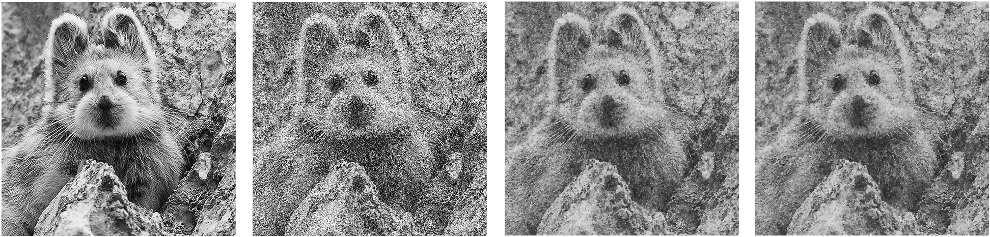
where we use super-script to avoid confusion with the finite training ground . Note that the training ground gives the original training scheme ((-L1)-(-L2)) with regularizer only. We perform numerical simulations of the images shown in Figure 1: the first image represents a clean image , whereas the second one is a noised version . We summarize our simulation results in Table 1 below.
| Training ground | optimal solution | minimum assessment value |
|---|---|---|
| 14.8575 | ||
| , | 12.8382 | |
| , , | 12.2369 |
We observe that, from Table 1, as the training ground expand, the minimum value of assessment function decreased. In another word, our new regularizer indeed provides an improved reconstructed result compare with regularizer. However, we remark that the extension of training ground results in a increasing of considerable large amount of CPU time, this would not be a big problem for practical application since we only need to use it one time for a given data set, and the structure of finite training ground allows us to use parallel computing very efficiently and hence reduce the CPU usage.
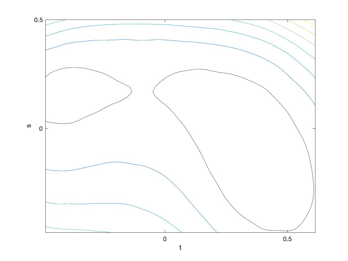
To explore the numerical landscapes of the assessment function with respect to , we consider the following training ground with intensity parameter fixed
| (5.6) |
and we plot in Figure 2 the mesh and contour images.

We remark that the introduction of regularizers into the training scheme is only meant to expand the training choices, but not to provide a superior semi-norm with respect to the standard semi-norm. The fact whether the optimal regularizer is or another intermediate regularizer, is completely dependent on the given training image . Moreover, we remark that the results discovered in this article are not restricted to the imaging processing problems only. It can be generally applied to parameter estimation problems of variational inequalities, as long as a suitable assessment function can be defined.
5.2. Further generalization of regularizer
5.2.1. Extension with variating underlying Euclidean norm
For , we recall that, for , the -Euclidean norm of is defined as
| (5.7) |
Note that for , we recovery the standard Euclidean norm , which is used in (2.8).
In the spirit of [22], we could generalize regularizer by variating the underlying Euclidean norm. To be precise, we define
| (5.8) |
where represents the dual norm of , as well as a new training scheme
| Level 1. | (-L1) | |||
| Level 2. | (-L2) |
with the training ground
| (5.9) |
We remark that, both Theorem 4.4 and Theorem 4.9 holds on this new training scheme with training ground and , respectively. The prove is identical to the argument presented before and the argument used in [22] when deal with parameter , so we decide to not report it here to avoid redundancy.
5.2.2. Extension with real order derivative
Let be given, we define the real -order operator by
| (5.10) |
where represent the order Hessian of . For example, for and , we have
| (5.11) |
where represent the Riemann-Liouville fractional partial derivative with order (see [18, Definition 2.6]). Then we define
| (5.12) |
and the new scheme
| Level 1. | (-L1) | |||
| Level 2. | (-L2) |
with training groud
| (5.13) |
We remark that Theorem 4.4 holds, with additional technics needed when deal with order parameter which we report separately in [19]. However, dual to the complexity of fractional order derivative, we can not directly deduce an analogously version of Theorem 4.9.
5.3. Upcoming works
In [9], a PDE-constraint total generalized variation, say , in multi-dimensions is defined as follows
| (5.14) |
where : is a first order differential operator with some natural PDE constraint (see Section 3 in [9]).
In our follow-up work, we propose to construct an unified approach to regularizers and via
| (5.15) |
We shall equip the training scheme with this new regularizer and provide an analogously version of Theorem 4.4 and Theorem 4.9 in our follow-up work.
Acknowledgments. PL acknowledges support from the EPSRC Centre Nr. EP/N014588/1 and the Leverhulme Trust project on Breaking the non-convexity barrier. The author also gratefully acknowledge the support of NVIDIA Corporation with the donation of a Quadro P6000 GPU used for this research.
References
- [1] T. Barbu and G. Marinoschi. Image denoising by a nonlinear control technique. International Journal of Control, 90:1005–1017, 2017.
- [2] M. Bergounioux. Optimal control of problems governed by abstract elliptic variational inequalities with state constraints. SIAM J. Control Optim., 36(1):273–289 (electronic), 1998.
- [3] K. Bredies, K. Kunisch, and T. Pock. Total generalized variation. SIAM J. Imaging Sci., 3(3):492–526, 2010.
- [4] D. Breit, L. Diening, and F. Gmeineder. Traces of functions of bounded a-variation and variational problems with linear growth. arXiv preprint arXiv:1707.06804, 2017.
- [5] H. Brezis. Functional analysis, Sobolev spaces and partial differential equations. Universitext. Springer, New York, 2011.
- [6] A. Chambolle and T. Pock. A first-order primal-dual algorithm for convex problems with applications to imaging. Journal of Mathematical Imaging and Vision, 40(1):120–145, 2011.
- [7] Y. Chen, T. Pock, R. Ranftl, and H. Bischof. Revisiting loss-specific training of filter-based mrfs for image restoration. In Pattern Recognition, pages 271–281. Springer, 2013.
- [8] Y. Chen, R. Ranftl, and T. Pock. Insights into analysis operator learning: From patch-based sparse models to higher order mrfs. IEEE Transactions on Image Processing, 23(3):1060–1072, March 2014.
- [9] E. Davoli, I. Fonseca, and P. Liu. Adaptive image processing: first order PDE constraint regularizers and a bilevel training scheme. arXiv.
- [10] E. Davoli and P. Liu. One dimensional fractional order tgv: gamma-convergence and bilevel training scheme. Commun. Math. Sci., 16(1):213–237, 2018.
- [11] J. C. De los Reyes and C.-B. Schönlieb. Image denoising: learning the noise model via nonsmooth PDE-constrained optimization. Inverse Probl. Imaging, 7(4):1183–1214, 2013.
- [12] J. Domke. Generic methods for optimization-based modeling. In AISTATS, volume 22, pages 318–326, 2012.
- [13] I. Ekeland and R. Temam. Convex analysis and variational problems. SIAM, 1976.
- [14] L. C. Evans and R. F. Gariepy. Measure theory and fine properties of functions. Studies in Advanced Mathematics. CRC Press, Boca Raton, FL, 1992.
- [15] I. Fonseca and S. Müller. Relaxation of quasiconvex functionals in for integrands . Arch. Rational Mech. Anal., 123(1):1–49, 1993.
- [16] K. C. Kiwiel. Convergence and efficiency of subgradient methods for quasiconvex minimization. Math. Program., 90(1, Ser. A):1–25, 2001.
- [17] K. Kunisch and T. Pock. A bilevel optimization approach for parameter learning in variational models. SIAM J. Imaging Sci., 6(2):938–983, 2013.
- [18] P. Liu and X. Y. Lu. Real order (an)-isotropic total variation in image processing - Part I: analytical analysis and functional properties. ArXiv e-prints, May 2018.
- [19] P. Liu and X. Y. Lu. Real order (an)-isotropic total variation in image processing - Part II: learning of optimal structures. ArXiv e-prints, 2019.
- [20] L. I. Rudin, S. Osher, and E. Fatemi. Nonlinear total variation based noise removal algorithms. Phys. D, 60(1-4):259–268, 1992. Experimental mathematics: computational issues in nonlinear science (Los Alamos, NM, 1991).
- [21] S. G. Samko, A. A. Kilbas, and O. I. Marichev. Fractional integrals and derivatives. Gordon and Breach Science Publishers, Yverdon, 1993. Theory and applications, Edited and with a foreword by S. M. Nikol\cprimeskiĭ, Translated from the 1987 Russian original, Revised by the authors.
- [22] C.-B. Schönlieb and P. Liu. Learning optimal orders of the underlying euclidean norm in total variation image processing. arXiv, 2018.
- [23] M. F. Tappen, C. Liu, E. H. Adelson, and W. T. Freeman. Learning gaussian conditional random fields for low-level vision. In 2007 IEEE Conference on Computer Vision and Pattern Recognition, pages 1–8, June 2007.